Shear viscosity: velocity gradient as a constraint on wave function

Abstract

By viewing a velocity gradient in a fluid as an internal disturbance and treating it as a constraint on the wave function of a system, a linear evolution equation for the wave function is obtained from the Lagrange multiplier method. It allows us to define the microscopic response to a velocity gradient in a pure state. Taking a spatial coarse-graining average over this microscopic response and averaging it over admissible initial states, we achieve the observed macroscopic response and transport coefficient. In this scheme, temporal coarse-graining is not needed. The dissipation caused by a velocity gradient depends on the square of initial occupation probability, whereas the dissipation caused by a mechanical perturbation depends on the initial occupation probability itself. We apply the method of variation of constants to solve the time-dependent Schrodinger equation with constraints. The various time scales appearing in the momentum transport are estimated. The relation between the present work and previous theories is discussed.

I Introduction

To express macroscopic observables in terms of the microscopic parameters of composite particles, one has to reduce an infinite number of mechanical degrees of freedom to a few hydrodynamical degrees of freedomdgr . Two typical techniques are projection and coarse-graining. In the projection method, one can either project the density matrix to a reduced density matrix for the relevant degrees of freedom (Schrodinger picture)zw60 ; kub or project a sum of microscopic mechanical variables to a macroscopic slow variable (Heisenberg picture)zw61 ; sew ; mo . While in the coarse-graining method, excepting the obligatory ensemble average, one still has to carry out at least one of three average procedures: (1) coarse-graining in timeka1 ; ori ; (2) coarse-graining in spacerus ; bins ; bi ; jac ; or (3) coarse-graining in the eigenvalue spectrum of energy and other collective variableska1 ; sew .

In the coarse-graining techniques, the spatial coarse grained average plays an essential role in formulating all macroscopic problems. Macroscopically, a non-equilibrium process in a fluid is described by some local hydrodynamic (thermodynamic, macroscopic) variables: temperature, stress, concentration and macroscopic velocity field etcdgr . The fundamental assumption behind this macroscopic description is that there exists a local equilibrium at each coarse-grained spatial ‘point’ and at every coarse-grained temporal ‘moment’dgr . Similarly in the kinetic theories, at least three of the arguments of the single-particle distribution function, time, position and translational momentum are defined in a coarse-grained sense (far more coarse-grained than the requirement of uncertainty principle)kub ; pk . As an alternative to the distribution function in phase space, Onsager introduced a distribution function for the coarse grained moments of the conserved quantities (displacements)on1 ; on2 . To obtain hydrodynamic equations and transport coefficients, M. S. Green noticed that the resolution of a macroscopic measurement is finite, so that one must eliminate the high wave number components of a collective variable which are are unmeasurable. The observed value of a hydrodynamic variable is given by averaging the truncatedbins ; bi collective variable over the distribution function of Markoff processmel1 ; mel2 .

It is well-known that temporal coarse-graining (TCG) is not necessary for deriving the macroscopic Maxwell equations (MAME) from the microscopic onesrus ; bins ; bi . A safe lower limit of length $L_{0}$ for a macroscopic description of reflection and refraction of visible light can be taken as $10^{2}$Åjac . The time scale $t_{0}$ associated with $L_{0}$ is in the range of atomic or molecular motions, a TCG at a time scale $t_{0}$ is meaninglessjac . Moreover, if one averages the motion of the particles over a time scale longer than $t_{0}$, the scattering phenomena will be smearedlv8 . In the MAME, the sources of fields are the total charge density and the total current densityjac ; lv8 . At the same time, the induced charge density and the induced current density are also the responses of the system to the external fields. Since no TCG is taken in deriving MAME, one should not require TCG in computing current density (conductivity)short ; pss ; 4t ; maw . The energy dissipation of system is taken care of by the thermal contact with a thermal bathcb ; maw ; jp . It seems that TCG is not needed for the irreversible processes caused by the mechanical distrubanceskyn ; k57 ; rus ; bins ; bi ; jac ; lv8 ; short ; pss ; 4t ; maw .

An open question is whether TCG is necessary to describe an irreversible process induced by an internal (thermal) disturbancekyn . Several schemes have been designed to replace an internal disturbance with a fictitious mechanical disturbanceoll ; kad ; lut ; maz ; fel . But these methods assume a priori that the Navier-Stokes equation is validzub . In other theories, TCG is often taken along with spatial coarse-graining and ensemble averagekyn ; kub ; zub ; eva ; cb ; ori . In particularly, TCG is viewed as a critical step producing irreversibility in the kinetic approach (master or Boltzmann equation)cb ; ka1 .

Although a velocity gradient is often viewed as an internal disturbance, it can be realized in a ‘mechanical’ manner. In a fluid, two obvious ways to produce a velocity gradient are (i) moving a boundary plate which confines the fluid; and (ii) stirring the fluid with a rod in the middle. In both situations, a velocity gradient is produced by the interaction between the fluid and an external object at the solid-fluid interface. A non-equilibrium ‘Hamiltonian’ has been phenomenologically introduced to effectively compute viscosityhoo ; ean ; eva . In addition, for a mechanical disturbancekyn ; k57 , one may define microscopic response in a pure state. The observed macroscopic response (consequently transport coefficient) is given by spatial coarse graining the microscopic response and averaging over possible initial conditionsshort ; pre ; jp ; pss . It is worthwhile to explore whether we could describe viscosity in a more ‘mechanical’ manner: (i) not invoking temporal coarse-graining; and (ii) not assuming local equilibrium as the starting point.

In this paper, we show that shear viscosity can be strictly calculated from a time-dependent Schrodinger equation, and time coarse-graining can be avoided. One may repeat the same procedure for bulk viscosity mutatis mutandis. In the discussion, we will only use the Schrodinger picture. Because a hydrodynamic quantity is a bilinear form of the many-body wave function, all the conclusions are valid for any set of identical particles: bosons or fermions. Only when we take concrete approximations for the many-body wave functions, do we need to know whether the particles are fermions or bosons.

In Sec. II, we first express the velocity gradient in a fluid as a constraint on the wave function of the fluid, cf. Eq.(16). To prescribe an internal disturbance like velocity gradient, one needs the wave function of the system. The wave function must be determined self-consistently with the given velocity gradient. With velocity gradient as a constraint, the evolution equation for wave function is then derived using the Lagrange multiplier methodcou , cf. Eqs.(23,24,25). From the appearance, it is a time-dependent Schrodinger equation. Two additional terms [Eqs.(24,25)] appear in the ‘Hamiltonian’. Both of them contain the occupation probabilities of admissible initial states, which reflects the fact that a velocity gradient is an internal disturbance. On the other hand a mechanical perturbation is completely specified by the time dependence of external fieldk57 .

In Sec. III, we first discuss the entropy production rate of the system + bath, cf. Eqs.(33,32). Secondly, we check the mass conservation law, cf. Eqs.(34,35). Thirdly, the microscopic response Eq.(37) to the velocity gradient (the momentum flux in a pure state) is obtained from the momentum conservation law in a pure state. The dissipation caused by a mechanical perturbation depends on the occupation probabilities of admissible initial states. Because a velocity gradient is an internal disturbance, the dissipation caused by a velocity gradient depends on the squares of the occupation probabilities of admissible initial states. This feature is clearly seen in the time rates of change of energy, mass and momentum.

Representing velocity gradient as a constraint on the wave function [Eq.(16)] depends critically on the assumption that a suitable spatial coarse-graining is adequaterus ; bins ; bi ; jac to describe internal friction. In Sec. IV we show that the spatial coarse-graining average automatically contains a coarse-graining in time [Eq.(42)] and a coarse-graining in eigenvalue spectrum of collective variables [Sec. IV.2].

In Sec. V, we apply the method of variation constants to obtain the Lagrange multipliers which appear in the solution of the time-dependent Schrodinger equation. The Lagrange multipliers characterize the interaction on the system exerted by the boundary plates. The phenomenological non-equilibrium ‘Hamiltonian’hoo ; ean ; eva can be obtained from $H_{d}$, the interaction of system with plates linear in velocity gradient. The shear viscosity is read from the macroscopic momentum flux (59) which is deduced from the wave function of system at some moment. In Sec. VI, we explain that applying Dirac perturbation theory to transport process is valid. Various time scales in the momentum transport process are discussed. We show that the length scale of spatial coarse-graining is determined by an intrinsic time scale.

In Sec. VII, we show that the macroscopic stress tensor derived from the microscopic response method is the same as that derived from averaging the momentum flux operator over the density matrix. We developed a cumulant expansion for the density operator. When we replace the operator in the exponent with its expectation value, we reproduce the non-equilibrium density matrix obtained from other approaches.

II evolution of state driven by velocity gradient

A mechanical disturbance on a system can be expressed by the coupling between the mechanical degrees of freedom of the system and some specified external parameters which may depend on time and position. The disturbance caused by a velocity gradient is more complicated. We will see that to describe a fluid with a velocity gradient, the occupation probabilities of admissible initial states enter the ‘Hamiltonian’ of the fluid. In Sec.II.1 we briefly summarize the microscopic response method for a mechanical perturbationshort ; pss ; jp ; pre . Later, we will show that one can still define a momentum flux in a pure state (microscopic response to velocity gradient), viscosity can be calculated from a modified time-dependent Schrodinger equation.

II.1 Macroscopic response to a mechanical disturbance

Consider a $N-$particle system $\mathcal{S}$ described by Hamiltonian $H_{0}$, we use indexes $a,b,\cdots$ to label the eigenvalues $\{E_{a}\}$ and eigenstates $\{\Phi_{a}\}$ of $H_{0}$:

$$H_{0}\Phi_{a}=E_{a}\Phi_{a}.$$ (1)

If the system $\mathcal{S}$ is in thermal contact with a thermal reservoir $\mathcal{B}$ at temperature $T$, and is in equilibrium with itcb ; fel , the probability that the system is in state $\Phi_{b}$ is

$$P^{\Phi_{b}}=e^{-E_{b}/k_{B}T}/\sum_{a}e^{-E_{a}/k_{B}T}.$$ (2)

Because the system is macroscopic, comparing the energy of system $\mathcal{S}$, the energy exchange rate between the system and the bath is slowv5 . In a time period much longer than a macroscopic measurement, the system can be viewed as isolated, and described by a wave function. For a macroscopic fluid, the detailed dynamics of the surrounding bath is not important.

If a mechanical disturbance described by Hamiltonian $H_{f}$ is exerted on $\mathcal{S}$, the state $\Psi$ of $\mathcal{S}$ will evolve according to

$$i\hbar\partial\Psi/\partial t=(H_{0}+H_{f})\Psi.$$ (3)

The above description requires thatcb ; jp $\mathcal{S}$ is in good thermal contact with $\mathcal{B}$ such that the energy generated by the disturbance $H_{f}$ inside $\mathcal{S}$ can be rapidly transferred into $\mathcal{B}$, and the system is maintained at the temperature $T$ of bath $\mathcal{B}$. If we assume that the system is initially in state $\Phi_{a}$, the state $\Psi_{a}(t)$ of system at time $t$ is determined by Eq.(3) with initial condition $\Psi_{a}(t=-\infty)=\Phi_{a}$. For convenience we adiabatically introduced $H_{f}$. By means of the microscopic conservation law in a pure state, we can defineshort the corresponding microscopic response (flux) in state $\Psi_{a}(t)$.

One can always spatially resolve a quantity $A^{\Psi_{a}}(\mathbf{R},t)$ in state $\Psi_{a}$ into its Fourier components:

$$A^{\Psi_{a}}(\mathbf{R},t)=\int\frac{d^{3}k}{(2\pi)^{3/2}}e^{i\mathbf{k}\cdot\mathbf{R}}\mathcal{A}^{\Psi_{a}}(\mathbf{k},t).$$ (4)

Because any instrument has finite spatial resolution, one can only detect those $\mathcal{A}^{\Psi_{a}}(\mathbf{k},t)$ with $|\mathbf{k}|<k_{0}$, where $k_{0}$ is some instrument limited cut-off wave numbermel2 ; rus ; bi . To express a macroscopic measurement, one has to make spatial coarse-grained averagebi ; jac :

$$A^{c\Psi_{a}}(\mathbf{r},t)=\int d\mathbf{R}f(\mathbf{r}-\mathbf{R})A^{\Psi_{a}}(\mathbf{R},t),$$ (5)

where $f(\mathbf{s})$ is any function satisfying: (1) $\int d\mathbf{s}f(\mathbf{s})=1$; and (2) the Fourier components of $f(\mathbf{s})$ tends rapidly to zero for $|\mathbf{k}|>k_{0}$. The integral in Eq.(5) is over the sample.

Since the system is in thermal contact with a reservoir, i.e. a member of a canonical ensemble, one does not know which state the system is initially in. The measured quantity is an ensemble average of $A^{\Psi_{a}c}(\mathbf{r},t)$:

$$A(\mathbf{r},t)=\sum_{\Psi_{a}}P^{\Phi_{a}}A^{c\Psi_{a}}(\mathbf{r},t),$$ (6)

where $P^{\Psi_{a}}(-\infty)=P^{\Phi_{a}}$ is the probability that the system is in state $\Psi_{a}(t=-\infty)=\Phi_{a}$ in the remote past. Since the microscopic response $A^{\Psi_{a}}(\mathbf{R},t)$ is a bilinear form of $\Psi_{a}$, it can be computed from Eq.(3) rather than from the Liouville equation for the density matrix. Since the spatial coarse-graining (5) and the average over initial conditions (6) do not involve the temporal evolution of the system, the macroscopic response $A(\mathbf{r},t)$ and consequently transport coefficient are also determined by the time-dependent Schrodinger equationcb ; short ; pss ; pre . The averaging procedure (5,6) is simpler than, and equivalent to Kubo’s linear response theorypre .

The procedure (5,6) aims at the steady states $\{\Psi_{a}(t)\}$ of $\mathcal{S}$ under a monochromatic driving. The general linear casual response to a disturbance with arbitrary time dependence will be discussed in Sec.VI.2.2.

II.2 Velocity gradient as a constraint on wave function

Consider a fluid composed of $N$ identical particles with mass $m$. We use indexes $j$, $k$, $l\cdots$ to label the particles. Denote the interaction energy between two particles at $\mathbf{r}_{k}$ and $\mathbf{r}_{l}$ as $U(\mathbf{r}_{k},\mathbf{r}_{l})$. Then the Hamiltonian of system is

$$H_{0}=-\frac{\hbar^{2}}{2m}\sum_{k=1}^{N}\nabla_{\mathbf{r}_{k}}^{2}+\frac{1}{2}\sum_{k,l(k\neq l)}U(\mathbf{r}_{k},\mathbf{r}_{l}).$$ (7)

Put the system in an external field, denote the interaction potential energy for a particle at $\mathbf{r}_{k}$ in the external field as $V(\mathbf{r}_{k},t)$. The interaction Hamiltonian with external field is

$$H_{f}=\sum_{k=1}^{N}V(\mathbf{r}_{k},t).$$ (8)

In the remote past $t=-\infty$, suppose that the system is in state $\Phi_{a}$. Driving the system with a velocity gradient and $H_{f}$, $\Phi_{a}$ will evolve into a state $\Psi_{a}(\mathbf{r}_{1}\cdots\mathbf{r}_{N};t)$ at time $t$. Eq.(2) indicates that we do not have the full knowledge of the system at the initial moment. The evolution of the system can then be understood to be probabilistictol . The interaction $U$ among molecules renders the macroscopic motion involving a velocity gradient irreversibletol .

II.2.1 Macroscopic velocity field in a fluid

Using the definition of mass density operator mel2 ; kub $\widehat{\rho}(\mathbf{r})=\sum_{j=1}^{N}m\delta(\mathbf{r}-\mathbf{r}_{j})$, the mass density for state $\Psi_{a}(t)$ is a function of time and position:

$$\rho^{\Psi_{a}}(\mathbf{r},t)=Nm\int d\tau_{1}\Psi_{a}^{\ast}\Psi_{a},$$ (9)

where $d\tau_{1}=d\mathbf{r}_{2}\cdots d\mathbf{r}_{N},$ the arguments of $\Psi_{a}$ are $(\mathbf{r},\mathbf{r}_{2},\mathbf{r}_{3},\cdots,\mathbf{r}_{N};t)$. The momentum density operator is defined asmel2 ; kub

$$\widehat{p}_{\gamma}(\mathbf{r})=\frac{1}{2}\sum_{j=1}^{N}[-i\hbar\frac{\partial}{\partial r_{j\gamma}}\delta(\mathbf{r}-\mathbf{r}_{j})+\delta(\mathbf{r}-\mathbf{r}_{j})(-i\hbar\frac{\partial}{\partial r_{j\gamma}})],$$ (10)

where $\gamma=x,y,z$ are indexes for three Cartesian components. The momentum density in state $\Psi_{a}$ is

$$S_{\gamma}^{\Psi_{a}}(\mathbf{r},t)=\frac{i\hbar}{2}N\int d\tau_{1}(\Psi_{a}\frac{\partial\Psi_{a}^{\ast}}{\partial r_{\gamma}}-\Psi_{a}^{\ast}\frac{\partial\Psi_{a}}{\partial r_{\gamma}}).$$ (11)

According to Eqs.(5,6), the measured macroscopic mass density is

$$\rho(\mathbf{r},t)=\sum_{\Psi_{a}}P^{\Phi_{a}}\int d\mathbf{R}f(\mathbf{r}-\mathbf{R})Nm\int d\tau_{1}\Psi_{a}\Psi_{a}^{\ast},$$ (12)

where the arguments of $\Psi_{a}$ are $(\mathbf{R},\mathbf{r}_{2},\mathbf{r}_{3},\cdots,\mathbf{r}_{N};t)$. The measured macroscopic momentum density is

$$S_{\gamma}(\mathbf{r},t)=\sum_{\Psi_{a}}P^{\Phi_{a}}\int d\mathbf{R}f(\mathbf{r}-\mathbf{R})S_{\gamma}^{\Psi_{a}}(\mathbf{R},t).$$ (13)

The macroscopic velocity field should be defined asmel2 ; ori ; v6 :

$$v_{\gamma}(\mathbf{r},t)=S_{\gamma}(\mathbf{r},t)/\rho(\mathbf{r},t),\text{ }\gamma=x,y,z.$$ (14)

It satisfies the requirement that the macroscopic velocity is the macroscopic momentum of unit mass of fluidv6 .

II.2.2 Velocity gradient

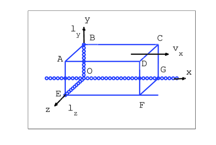
Figure 1: Experimental setup for velocity gradient: the top plates ABCD moves toward $+x$ direction (right) with speed $v_{x0}$. The bottom OEFG, front (right) bank AEFD and back (left) bank BOGC are static. The width of channel is $l_{z}$, the depth of channel is $l_{y}$.

We first describe the simplest experimental setup for measuring shear viscosity in Fig.1. Let the fluid flow in a rectangular channel along the $x$ direction. We choose a coordinate system such that the two banks BOGC and AEFD of the channel are $z=0$ and $z=l_{z}$, the bottom surface OEFG of channel is $y=0$, the top surface ABCD of the fluid is bordered by a plate $y=l_{y}$ with velocity $v_{x0}$. The points on the bottom plate OEFG are denoted as $\mathbf{r}^{(1)}(x,0,z)$ with $-\infty<x<\infty$ and $0<z<l_{z}$, the boundary condition on bottom is $v_{\gamma}(\mathbf{r}^{(1)},t)=0$, $\gamma=x,y,z$. The points on the top plate ABCD are denoted as $\mathbf{r}^{(2)}(x,l_{y},z)$ with $-\infty<x<\infty$ and $0<z<l_{z}$, the boundary condition on the top plate is $v_{x}(\mathbf{r}^{(2)},t)=v_{x0},v_{y}(\mathbf{r}^{(2)},t)=v_{z}(\mathbf{r}^{(2)},t)=0$. The points on the back (left) bank BOGC of channel are denoted as $\mathbf{r}^{(3)}(x,y,0)$ with $-\infty<x<\infty$ and $0<y<l_{y}$, the boundary condition on the back bank BOGC is $v_{\gamma}(\mathbf{r}^{(3)},t)=0$, $\gamma=x,y,z$. The points on the front (right) bank AEFD of channel are denoted as $\mathbf{r}^{(4)}(x,y,l_{z})$ with $-\infty<x<\infty$ and $0<y<l_{y}$, the boundary condition on the front bank AEFD is $v_{\gamma}(\mathbf{r}^{(4)},t)=0$, $\gamma=x,y,z$. These no-slip conditions for a viscous fluid are the boundary conditions for the Navier-Stokes equationsv6 . We imposed a velocity gradient $v_{x0}/l_{y}$ in the fluid.

II.2.3 Velocity gradient as constraints on wave function

To enforce a velocity gradient as a constraint on the wave function, it is helpful to allow an arbitrary velocity field on each boundary surface. We use a two dimensional mesh to characterize the positions of the points on a boundary surface. For a point on the $\sigma^{th}$ plate ($\sigma=1,2,3,4$), we use two indexes $\mu_{\sigma}$ and $\nu_{\sigma}$ to describe its position, where $\mu_{\sigma}=1,2,\cdots,M_{1\sigma}$ and $\nu_{\sigma}=1,2,\cdots,M_{2\sigma}$. Thus the position vector of a point on the $\sigma^{th}$ plate with indexes $\mu_{\sigma}$ and $\nu_{\sigma}$ is denoted as $\mathbf{r}_{\mu_{\sigma}\nu_{\sigma}}^{(\sigma)}$, there are $M_{1\sigma}\times M_{2\sigma}$ points on the $\sigma^{th}$ boundary surface. A general velocity field on the $\sigma^{th}$ boundary surface may be specified $v_{\gamma}(\mathbf{r}_{\mu_{\sigma}\nu_{\sigma}}^{(\sigma)},t)$, $\gamma=x,y,z$. In terms of Eq.(14), the boundary condition on the $\sigma^{th}$ boundary surface is expressed as

$$S_{\gamma}(\mathbf{r}_{\mu_{\sigma}\nu_{\sigma}}^{(\sigma)},t)-\rho(\mathbf{r}_{\mu_{\sigma}\nu_{\sigma}}^{(\sigma)},t)v_{\gamma}(\mathbf{r}_{\mu_{\sigma}\nu_{\sigma}}^{(\sigma)},t)=0,$$ (15)

where $v_{\gamma}(\mathbf{r}_{\mu_{\sigma}\nu_{\sigma}}^{(\sigma)},t)$ is a know function of $(\mathbf{r}_{\mu_{\sigma}\nu_{\sigma}}^{(\sigma)},t)$. Making use of Eqs.(12,11,13), Eq.(15) becomes

$$\sum_{\Psi_{b}}P^{\Phi_{b}}\int d\mathbf{R}f(\mathbf{r}_{\mu_{\sigma}\nu_{\sigma}}^{(\sigma)}-\mathbf{R})N\int d\tau_{1}$$ (16)

$$\times[\frac{i\hbar}{2}(\Psi_{b}\frac{\partial\Psi_{b}^{\ast}}{\partial R_{\gamma}}-\Psi_{b}^{\ast}\frac{\partial\Psi_{b}}{\partial R_{\gamma}})-v_{\gamma}(\mathbf{r}_{\mu_{\sigma}\nu_{\sigma}}^{(\sigma)},t)m\Psi_{b}\Psi_{b}^{\ast}]=0.$$

Eq.(16) represents $M_{c}=3\times 4\times M_{1\sigma}\times M_{2\sigma}$ constraints on the wave function of system. The evolution equation of $\Psi_{a}(t)$ has to be modified with constraints (16).

II.3 Evolution of state in a velocity gradient

To consider the effect of constraints (16) on the state $\Psi_{a}$ of the many-particle system, we first notice that the Schrodinger equation

$$i\hbar\Psi_{at}=(H_{0}+H_{f})\Psi_{a}$$ (17)

is the Euler equation $\delta S/\delta\Psi_{a}^{\ast}=0$ of the actioncou ; if :

$$S=\int_{t_{1}}^{t_{2}}dt\int d\tau\mathcal{L}(\Psi_{a},\Psi_{at},\Psi_{a\mathbf{r}_{j}};\Psi_{a}^{\ast},\Psi_{at}^{\ast},\Psi_{a\mathbf{r}_{j}}^{\ast}),$$ (18)

where $\Psi_{at}=\partial\Psi_{a}/\partial t$, $\Psi_{a\mathbf{r}_{j}}=\nabla_{\mathbf{r}_{j}}\Psi_{a}$, $d\tau=d\mathbf{r}_{1}d\mathbf{r}_{2}\cdots d\mathbf{r}_{N}$ is the volume element in configurational space, the arguments of $\Psi_{a}$ are $(\mathbf{r}_{1},\mathbf{r}_{2},\cdots,\mathbf{r}_{N};t)$. The well-known Lagrangian density for Eq.(17) isif :

$$\mathcal{L}=i\hbar\Psi_{a}^{\ast}\Psi_{at}-\sum_{j=1}^{N}\frac{\hbar^{2}}{2m}\Psi_{a\mathbf{r}_{j}}^{\ast}\Psi_{a\mathbf{r}_{j}}$$ (19)

$$-[\sum_{k=1}^{N}V(\mathbf{r}_{k},t)+\frac{1}{2}\sum_{k,l(k\neq l)}U(\mathbf{r}_{k},\mathbf{r}_{l})]\Psi_{a}^{\ast}\Psi_{a}.$$

We apply the Lagrange multiplier methodcou to find the evolution equation of $\Psi_{a}(t)$ driven by a velocity gradient specified by Eq.(16). First of all we symmetrize Eq.(16) respect to all particles. Secondly, we multiply the expression with $\lambda_{\mu_{\sigma}\nu_{\sigma}}^{\gamma(\sigma)}(t)$ and integrate it over the time intervalzos $[t_{1},t_{2}]$:

$$\int_{t_{1}}^{t_{2}}dt\sum_{\Psi_{b}}P^{\Phi_{b}}\int d\mathbf{R}f(\mathbf{r}_{\mu_{\sigma}\nu_{\sigma}}^{(\sigma)}-\mathbf{R})$$

$$\lambda_{\mu_{\sigma}\nu_{\sigma}}^{\gamma(\sigma)}(t)\int d\tau\sum_{j=1}^{N}\delta(\mathbf{r}_{j}-\mathbf{R})[\frac{i\hbar}{2}(\Psi_{b}\frac{\partial\Psi_{b}^{\ast}}{\partial r_{j\gamma}}-\Psi_{b}^{\ast}\frac{\partial\Psi_{b}}{\partial r_{j\gamma}})$$

$$-mv_{\gamma}(\mathbf{r}_{\mu_{\sigma}\nu_{\sigma}}^{(\sigma)},t)\Psi_{b}\Psi_{b}^{\ast}]=0,$$ (20)

where the $\delta$ function is produced when we change $\int d\tau_{1}$ in Eq.(16) to $\int d\tau$ in Eq.(20). The macroscopic velocity at every point on each plate is a constraint. The overall Lagrangian density including the constraint (20) is

$$\mathcal{L}^{c}=\mathcal{L}+\sum_{\gamma\sigma\mu_{\sigma}\nu_{\sigma}}\lambda_{\mu_{\sigma}\nu_{\sigma}}^{\gamma(\sigma)}(t)\sum_{\Psi_{b}}P^{\Phi_{b}}\int d\mathbf{R}$$ (21)

$$f(\mathbf{r}_{\mu_{\sigma}\nu_{\sigma}}^{(\sigma)}-\mathbf{R})\sum_{j=1}^{N}\delta(\mathbf{r}_{j}-\mathbf{R})$$

$$[\frac{i\hbar}{2}(\Psi_{b}\frac{\partial\Psi_{b}^{\ast}}{\partial r_{j\gamma}}-\Psi_{b}^{\ast}\frac{\partial\Psi_{b}}{\partial r_{j\gamma}})-mv_{\gamma}(\mathbf{r}_{\mu_{\sigma}\nu_{\sigma}}^{(\sigma)},t)\Psi_{b}\Psi_{b}^{\ast}]$$

where the Lagrange multiplier $\lambda_{\mu_{\sigma}\nu_{\sigma}}^{\gamma(\sigma)}(t)$ is a real function of timezos with dimension length${}^{4}\cdot$time^-1. Roughly speaking, $\lambda_{\mu_{\sigma}\nu_{\sigma}}^{\gamma(\sigma)}(t)$ is a product of the $\gamma^{th}$ component of velocity at point $\mathbf{r}_{\mu_{\sigma}\nu_{\sigma}}^{(\sigma)}$ of the $\sigma^{th}$ plate and the disturbed volume of fluid by a molecule at $\mathbf{r}_{\mu_{\sigma}\nu_{\sigma}}^{(\sigma)}$. We will see this in more detail in Sec.V.1.

The equation of motion for $\Psi_{a}(t)$ can be obtained from the Euler equation:

$$\frac{\partial\mathcal{L}^{c}}{\partial\Psi_{a}^{\ast}}-\sum_{j=1}^{N}\nabla_{\mathbf{r}_{j}}\frac{\partial\mathcal{L}^{c}}{\partial\Psi_{a\mathbf{r}_{j}}^{\ast}}-\frac{\partial}{\partial t}\frac{\partial\mathcal{L}^{c}}{\partial\Psi_{at}^{\ast}}=0.$$ (22)

It is

$$i\hbar\Psi_{at}=(H_{0}+H_{f}+H_{c}+H_{d})\Psi_{a},$$ (23)

where

$$H_{c}=P^{\Phi_{a}}\sum_{\gamma\sigma\mu_{\sigma}\nu_{\sigma}}\lambda_{\mu_{\sigma}\nu_{\sigma}}^{\gamma(\sigma)}(t)\int d\mathbf{R}f(\mathbf{r}^{(\sigma)}-\mathbf{R})$$ (24)

$$\times\sum_{j=1}^{N}\delta(\mathbf{r}_{j}-\mathbf{R})mv_{\gamma}(\mathbf{r}_{\mu_{\sigma}\nu_{\sigma}}^{(\sigma)},t),$$

and

$$H_{d}=P^{\Phi_{a}}\sum_{\gamma\sigma\mu_{\sigma}\nu_{\sigma}}\lambda_{\mu_{\sigma}\nu_{\sigma}}^{\gamma(\sigma)}(t)\int d\mathbf{R}f(\mathbf{r}_{\mu_{\sigma}\nu_{\sigma}}^{(\sigma)}-\mathbf{R})$$

$$\times\sum_{j=1}^{N}\{\delta(\mathbf{r}_{j}-\mathbf{R})i\hbar\frac{\partial}{\partial r_{j\gamma}}+\frac{i\hbar}{2}\frac{\partial\delta(\mathbf{r}_{j}-\mathbf{R})}{\partial r_{j\gamma}}\}.$$ (25)

One may notice that Eq.(23) contains only $\Psi_{a}$ and its partial derivatives. Other $\Psi_{b}$ do not appear. In this sense, the velocity gradient is a special mechanical perturbation. On the other hand, the solution $\Psi_{a}(t)$ of Eq.(23) involves $M_{c}$ parameters $\{\lambda_{\mu_{\sigma}\nu_{\sigma}}^{\gamma(\sigma)}(t)\}$, that should also satisfy $M_{c}$ constraints (16) which mix all $\{\Psi_{b}(t)\}$. Thus velocity gradient is also an internal disturbancekub ; kyn .

In $H_{c}$ and $H_{d}$, the integrals behind the summation signs are the macroscopic momentum density and negative momentum density operator respectively. Thus the subtracted momentum density automatically happenspic in $H_{c}+H_{d}$ , which has to be introduced in some previous theoriesori .

Because $H_{d}\neq H_{d}^{\ast}$, one cannot find a system with wave function $\Psi^{\prime}(\{\mathbf{r}_{j}\};t)=\Psi_{a}^{\ast}(\{\mathbf{r}_{j}\};-t)$ such that $i\hbar\partial\Psi^{\prime}/\partial t=(H_{0}+H_{f}+H_{c}+H_{d})\Psi^{\prime}$, so that the process described by Eq.(23) is irreversibletol .

In classical mechanics, constraints can also be dealt with the Lagrange multiplier methodwhi ; zos ; gant ; pars . A constraint produces a reaction force on each particle in the system. The constraints (16) enforce the interaction on the system from four the plates.

Defining the macroscopic velocity field of a fluid by Eq.(14) has a profound consequence: the resultant constraint (16) on wave function is bilinear. The evolution equation (23) for $\Psi_{a}(t)$ is linear and does not include other states. The evolution of the state of system driven by a velocity gradient is almost determined in the framework of pure mechanics. If we had defined the macroscopic velocity field of fluid as

$$v_{\gamma}(\mathbf{r},t)=\sum_{\Psi_{a}}P^{\Phi_{a}}\int d\mathbf{R}f(\mathbf{r}-\mathbf{R})v_{\gamma}^{\Psi_{a}}(\mathbf{R},t),$$ (26)

with

$$v_{\gamma}^{\Psi_{a}}(\mathbf{R},t)=S_{\gamma}^{\Psi_{a}}(\mathbf{R},t)/\rho^{\Psi_{a}}(\mathbf{R},t),$$ (27)

we would have two serious difficulties: (i) this definition breaks the basic requirement that the macroscopic mass flux density $S_{\gamma}(\mathbf{r},t)$ must always be the macroscopic momentum of unit volume of fluidv6 ; (ii) the resulted temporal evolution equation for $\Psi_{a}(t)$ is nonlinear, and $\Psi_{a}(t)$ couples with other $\{\Psi_{b}(t)\}$. Certainly, assuming the fluid is incompressible, the labyrinthine evolution equations could be linearized and decoupled.

II.4 A comparison of velocity gradient and a mechanical disturbance

For a mechanical perturbation, external fields are some specified functions of time. The interaction Hamiltonian $H_{f}$ is expressed by the external fields, the coordinate and momentum operators of all particleskyn ; short ; jp . The states $\{\Psi_{a}(t)\}$ of system are not involved in $H_{f}$. On the other hand, the macroscopic velocity field of a fluid is defined in Eq.(14) through macroscopic mass density (12) and macroscopic mass flux (13). The later two quantities involve the states $\{\Psi_{a}(t)\}$ of system, spatial coarse-graining and average over various initial conditions. Before specifying the velocity gradient, which involves the states $\{\Psi_{a}(t)\}$ of system, we cannot determine the evolution of the state of system driven by a velocity gradient.

From the charge conservation law in a pure state, one can directly use the time-dependent Schrodinger equation (3) to deriveshort ; pss the current density $\mathbf{j}^{\Psi_{a}}(\mathbf{r},t)$ in state $\Psi_{a}$ (the microscopic response) from the temporal change of charge density $\rho^{\Psi_{a}}(\mathbf{r},t)$ in state $\Psi_{a}(t)$. One does not need the quantal operator of current densitypre , although the results are the same from the two points of view. In contrast, we cannot use mass conservation in a pure state to derive mass flux $S_{\gamma}^{\Psi_{a}}(\mathbf{r},t)$ in state $\Psi_{a}(t)$. We have to invoke the definition of momentum density (10). In this sense, the velocity gradient is an internal disturbancekub ; kyn . The states $\{\Psi_{a}(t)\}$ of system driven by velocity gradient have to be determined by the equation of motion (23) and the constraints (16) self-consistently.

III Conservation laws in a pure state

In this section, we assume that $\lambda_{\mu_{\sigma}\nu_{\sigma}}^{\gamma(\sigma)}(t)$ and $\{\Psi_{b}(t)\}$ are known. The time rate of change of energy, mass density and momentum density are derived. These relations are formal but exact. We will find $\lambda_{\mu_{\sigma}\nu_{\sigma}}^{\gamma(\sigma)}(t)$ and $\{\Psi_{b}(t)\}$ in Sec.V.

III.1 Time rate of change of total energy

The temporal or spatial change in local energy density is closely related to the temperature gradient. Since $\mathcal{S}$ is a member of the canonical ensemble at temperature $T$, we cannot talk about the time rate of change of local energy density.

For an isolated system $\mathcal{S}$, the total energy is conserved:

$$E^{\Phi_{a}}(t)=\int d\tau e^{itE_{a}/\hbar}\Phi_{a}^{\ast}H_{0}\Phi_{a}e^{-itE_{a}/\hbar}=E_{a}.$$ (28)

Consider a more general state of isolated system $\mathcal{S}$ with initial value $\Psi(0)=\sum_{e}c_{e}\Phi_{e}$, where $\{c_{e}\}$ are some constants. The time evolution of $\Psi(0)$ is $\Psi(t)=\sum_{e}c_{e}\Phi_{e}e^{-iE_{e}t/\hbar}$. From the orthogonality of eigenfunctions of $H_{0}$, it is easy to check that the average energy of $\Psi(t)$ is conserved:

$$E^{\Psi(0)}=\int d\tau\Psi^{\ast}(0)H_{0}\Psi(0)=\sum_{e}|c_{e}|^{2}E_{e},$$ (29)

and

$$E^{\Psi(t)}=\int d\tau\Psi^{\ast}(t)H_{0}\Psi(t)=\sum_{e}|c_{e}|^{2}E_{e}.$$ (30)

Now assume that the system $\mathcal{S}$ is in good contact with a thermal reservoir $\mathcal{B}$ in temperature $T$. Thus, even if we apply a velocity gradient and an external field on the system, $\mathcal{S}$ is maintained at the same temperature $T$. Because $\mathcal{S}$ is macroscopic, in a time period much longer than a macroscopic measurement, $\mathcal{S}$ can be viewed as quasi-closedv5 . Therefore we can use a wave function $\Psi_{a}(t)$ to describe the system. The average energy of $\mathcal{S}$ in state $\Psi_{a}(t)$ is defined as

$$E^{\Psi_{a}}(t)=\int d\tau\Psi_{a}^{\ast}(t)H_{0}\Psi_{a}(t).$$ (31)

Because $\Psi_{a}(t)$ satisfies Eq.(23), one can get the time rate of change $dE^{\Psi_{a}}(t)/dt$ of the energy $E^{\Psi_{a}}(t)$ in pure state $\Psi_{a}(t)$. The average energy $E(t)$ of $\mathcal{S}$ at time $t$ is $E(t)=\sum_{\Psi_{a}}P^{\Phi_{a}}E^{\Psi_{a}}(t)$. The time rate of energy exchange $dE(t)/dt$ between $\mathcal{S}$ and $\mathcal{B}$ is determined by

$$\frac{dE(t)}{dt}=\int d\mathbf{R}V(\mathbf{R},t)\nabla_{\mathbf{R}}\cdot$$ (32)

$$\sum_{a}P^{\Phi_{a}}\frac{i\hbar}{2m}N\int d\tau_{1}(\Psi_{a}\nabla_{\mathbf{R}}\Psi_{a}^{\ast}-\Psi_{a}^{\ast}\nabla_{\mathbf{R}}\Psi_{a})$$

$$-\sum_{\gamma\sigma\mu_{\sigma}\nu_{\sigma}}\lambda_{\mu_{\sigma}\nu_{\sigma}}^{\gamma(\sigma)}\int d\mathbf{R}f(\mathbf{r}_{\mu_{\sigma}\nu_{\sigma}}^{(\sigma)}-\mathbf{R})\frac{i\hbar}{2}\frac{\partial}{\partial R_{\gamma}}\nabla_{\mathbf{R}}\cdot$$

$$\sum_{a}(P^{\Phi_{a}})^{2}\frac{i\hbar}{2m}N\int d\tau_{1}(\Psi_{a}\nabla_{\mathbf{R}}\Psi_{a}^{\ast}-\Psi_{a}^{\ast}\nabla_{\mathbf{R}}\Psi_{a})$$

$$+\sum_{\gamma\sigma\mu_{\sigma}\nu_{\sigma}}\lambda_{\mu_{\sigma}\nu_{\sigma}}^{\gamma(\sigma)}\int d\mathbf{R}f(\mathbf{r}_{\mu_{\sigma}\nu_{\sigma}}^{(\sigma)}-\mathbf{R})mv_{\gamma}(\mathbf{r}_{\mu_{\sigma}\nu_{\sigma}}^{(\sigma)},t)\nabla_{\mathbf{R}}\cdot$$

$$\sum_{a}(P^{\Phi_{a}})^{2}\frac{i\hbar}{2m}N\int d\tau_{1}(\Psi_{a}\nabla_{\mathbf{R}}\Psi_{a}^{\ast}-\Psi_{a}^{\ast}\nabla_{\mathbf{R}}\Psi_{a})$$

$$+\sum_{\gamma\sigma\mu_{\sigma}\nu_{\sigma}}\lambda_{\mu_{\sigma}\nu_{\sigma}}^{\gamma(\sigma)}\int d\mathbf{R}f(\mathbf{r}_{\mu_{\sigma}\nu_{\sigma}}^{(\sigma)}-\mathbf{R})N\frac{i\hbar}{2}\nabla_{\mathbf{R}}\cdot$$

$$\sum_{a}(P^{\Phi_{a}})^{2}\frac{i\hbar}{2m}\int d\tau_{1}(\frac{\partial\Psi_{a}}{\partial R_{\gamma}}\nabla_{\mathbf{R}}\Psi_{a}^{\ast}-\Psi_{a}^{\ast}\nabla_{\mathbf{R}}\frac{\partial\Psi_{a}}{\partial R_{\gamma}})$$

$$-\sum_{\gamma\sigma\mu_{\sigma}\nu_{\sigma}}\lambda_{\mu_{\sigma}\nu_{\sigma}}^{\gamma(\sigma)}\int d\mathbf{R}f(\mathbf{r}_{\mu_{\sigma}\nu_{\sigma}}^{(\sigma)}-\mathbf{R})N(N-1)$$

$$\sum_{a}(P^{\Phi_{a}})^{2}\int d\tau_{1}U(\mathbf{R},\mathbf{r}_{2})\frac{\partial(\Psi_{a}\Psi_{a}^{\ast})}{\partial r_{2\gamma}},$$

where the arguments of $\Psi_{a}$ are$\ (\mathbf{R},\mathbf{r}_{2},\cdots,\mathbf{r}_{N};t)$. The last term is the power of the internal force near the boundary surfaces. In classical mechanics, for a group of particles, the internal forces do work on the systemqin . Only for a rigid body, is the work done by internal forces zero. It is interesting to notice that only for the regions close to the boundary plates [$f(\mathbf{r}_{\mu_{\sigma}\nu_{\sigma}}^{(\sigma)}-\mathbf{R})$ decays very rapidly when $|\mathbf{r}_{\mu_{\sigma}\nu_{\sigma}}^{(\sigma)}-\mathbf{R}|>k_{0}^{-1}$], the internal forces do work.

In Eq.(32), we can see an obvious distinction between a velocity gradient and a mechanical perturbation. The first term contains $P^{\Phi_{a}}$, is the power due to the external field. The remaining terms contains $[P^{\Phi_{a}}]^{2}$, the square of the occupation probability of admissible initial states. They are the contributions to power due to the friction at boundary surfaces. The first $P^{\Phi_{a}}$ comes from prescribing the macroscopic boundary condition as constraints on the wave function of a pure state. The interaction with plates are expressed by $H_{c}+H_{d}$ in the ‘Hamiltonian’ of system, cf. Eqs.(24,25). Since $dE^{\Psi_{a}}(t)/dt$ is determined by $\Psi_{at}(t)$, from Eq.(22), $dE^{\Psi_{a}}(t)/dt$ includes a $P^{\Phi_{a}}$. To obtain $dE(t)/dt$ from $dE^{\Psi_{a}}(t)/dt$, the average about possible initial states (6) introduced the second $P^{\Phi_{a}}$.

The temperature of $\mathcal{S}$ is maintained at $T$ by the bath $\mathcal{B}$. All the energy generated in the system is transferred to $\mathcal{B}$. The entropy $S^{\mathcal{B}}(t)$ of the bath $\mathcal{B}$ increases with time according to

$$dS^{\mathcal{B}}(t)/dt=T^{-1}dE(t)/dt.$$ (33)

Substituting Eq.(32) into Eq.(33) and noticing that $\lambda_{\mu_{\sigma}\nu_{\sigma}}^{\gamma(\sigma)}(t)f(\mathbf{r}_{\mu_{\sigma}\nu_{\sigma}}^{(\sigma)}-\mathbf{R})$ has dimension of velocity, each term is in the form of temperature^-1 $\times$velocity$\times$momentum$\times$velocity gradient, except the first and last term. This is consistent with the macroscopic law of entropy production ratev6 .

III.2 Time rate of change of mass density

With the help of Eq.(23), one may calculate the time rate of changeir50 ; ori of $\rho^{\Psi_{a}}(\mathbf{r},t)$. Further applying the averaging procedure (5,6) to the expression for $\partial\rho^{\Psi_{a}}(\mathbf{r},t)/\partial t$, one obtains the macroscopic law of mass conservation:

$$\frac{\partial\rho(\mathbf{r},t)}{\partial t}+\sum_{\gamma}\frac{\partial S_{\gamma}^{\prime}(\mathbf{r},t)}{\partial r_{\gamma}}=0,$$ (34)

where

$$S_{\gamma}^{\prime}(\mathbf{r},t)=S_{\gamma}(\mathbf{r},t)-\int d\mathbf{R}^{\prime}f(\mathbf{r}-\mathbf{R}^{\prime})\sum_{\sigma\mu_{\sigma}\nu_{\sigma}}\lambda_{\mu_{\sigma}\nu_{\sigma}}^{\gamma(\sigma)}$$ (35)

$$\times f(\mathbf{r}_{\mu_{\sigma}\nu_{\sigma}}^{(\sigma)}-\mathbf{R}^{\prime})\sum_{\Psi_{a}}[P^{\Phi_{a}}]^{2}\rho^{\Psi_{a}}(\mathbf{R}^{\prime},t).$$

In the R.H.S of Eq.(35), the first term $S_{\gamma}(\mathbf{r},t)$ is the usual macroscopic mass flux, and is given by Eq.(13). The second term is an additional mass flux caused by the given velocity gradient. Two truncation functionsmel2 ; bi $f(\mathbf{r}_{\mu_{\sigma}\nu_{\sigma}}^{(\sigma)}-\mathbf{R}^{\prime})$ and $f(\mathbf{r}-\mathbf{R}^{\prime})$ indicate that the correction is nonzero only near the boundary surfaces. Again, $[P^{\Phi_{a}}]^{2}$ reflects the fact that a velocity gradient is an internal disturbance.

III.3 Microscopic response: momentum flux in a pure state

Taking the time derivative of Eq.(11), one obtains the time rate of change of the momentum densityir50 ; ori $S_{\alpha}^{\Psi_{a}}(\mathbf{r},t)$ in state $\Psi_{a}(t)$. In terms of Eq.(23), one has:

$$\frac{\partial S_{\alpha}^{\Psi_{a}}(\mathbf{r},t)}{\partial t}+\sum_{\beta}\frac{\partial\Pi_{\alpha\beta}^{\Psi_{a}}(\mathbf{r},t)}{\partial r_{\beta}}=-\frac{\partial V(\mathbf{r},t)}{\partial r_{\alpha}}\rho^{\Psi_{a}}(\mathbf{r},t)/m$$ (36)

$$+P^{\Phi_{a}}\sum_{\gamma\sigma\mu_{\sigma}\nu_{\sigma}}\lambda_{\mu_{\sigma}\nu_{\sigma}}^{\gamma(\sigma)}(t)\frac{\partial f(\mathbf{r}_{\mu_{\sigma}\nu_{\sigma}}^{(\sigma)}-\mathbf{r})}{\partial r_{\alpha}}$$

$$\times[S_{\gamma}^{\Psi_{a}}(\mathbf{r},t)-v_{\gamma}(\mathbf{r}_{\mu_{\sigma}\nu_{\sigma}}^{(\sigma)},t)\rho^{\Psi_{a}}(\mathbf{r},t)],$$

where $\alpha,$ $\beta,$ $\gamma=x,y,z$, and the momentum flux $\Pi_{\alpha\beta}^{\Psi_{a}}(\mathbf{r},t)$ in state $\Psi_{a}$ is

$$\Pi_{\alpha\beta}^{\Psi_{a}}(\mathbf{r},t)=\frac{\hbar^{2}}{2m}N\int d\tau_{1}$$ (37)

$$[\frac{\partial\Psi_{a}}{\partial r_{\alpha}}\frac{\partial\Psi_{a}^{\ast}}{\partial r_{\beta}}+\frac{\partial\Psi_{a}^{\ast}}{\partial r_{\alpha}}\frac{\partial\Psi_{a}}{\partial r_{\beta}}-\frac{1}{2}\frac{\partial^{2}(\Psi_{a}\Psi_{a}^{\ast})}{\partial r_{\beta}\partial r_{\alpha}}]$$

$$-\frac{1}{2}N\int d\tau_{1}\sum_{k=2}^{N}(\mathbf{r}_{\beta}-\mathbf{r}_{k\beta})\frac{\partial U(\mathbf{r}_{k},\mathbf{r})}{\partial r_{\alpha}}\Psi_{a}\Psi_{a}^{\ast}.$$

In Eq.(37), the arguments of $\Psi_{a}$ are $(\mathbf{r},\mathbf{r}_{2}\cdots\mathbf{r}_{N};t)$. To obtain the divergence form for the second term in Eq.(37), we used the fact that the range of interaction force is much shorter thanmel2 ; zub $k_{0}^{-1}$.

Although velocity gradient is an internal disturbance, by viewing the velocity gradient as a constraint on the wave function, one can still define a microscopic response: the momentum flux $\Pi_{\alpha\beta}^{\Psi_{a}}$ in state $\Psi_{a}(t)$. Applying Eqs.(5,6), one obtains the measured macroscopic momentum flux:

$$\Pi_{\alpha\beta}(\mathbf{r},t)=\sum_{\Psi_{a}}P^{\Phi_{a}}\int d\mathbf{R}f(\mathbf{r}-\mathbf{R})\Pi_{\alpha\beta}^{\Psi_{a}}(\mathbf{R},t).$$ (38)

After $\Psi_{a}(t)$ is obtained, the shear viscosity can be read out from Eqs.(37,38).

In the RHS of Eq.(36), the first term is the momentum density produced by the external field per unit time, the second term is the momentum density produced by the constraint (16) per unit time. Because the moving plate drives the fluid, $\mathcal{S}$ gains momentum and energy. Thus there are source terms in the equations for the time rate of change, cf. Eqs. (36) and (32). Since no mass is produced by a velocity gradient, there is not a source term in the time rate of change of mass density, cf. Eq.(34).

There is a subtle difference between Eqs.(36,37) and the corresponding results in previous theoriesmac1 ; mac2 ; mel2 ; zub ; rob ; rob66 ; rob67 ; pic ; ir50 ; ir51 . In all previous theories, conservation laws and fluxes (responses) are derived for an isolated fluid system without imposing velocity gradient. The system satisfies

$$i\hbar\partial\Psi_{0}/\partial t=H_{0}\Psi_{0}$$ (39)

or Newton’s equation for an isolated systemmel2 ; zub ; rob ; rob66 ; rob67 ; pic ; ir50 ; ir51 . The operator of momentum flux isori ; ir50 ; ir51 ; rob

$$\widehat{\Pi}_{\alpha\beta}(\mathbf{r})=\sum_{i=1}^{N}\frac{1}{4m}\{p_{\alpha}^{i}p_{\beta}^{i}\delta(\mathbf{r}_{i}-\mathbf{r})+p_{\alpha}^{i}\delta(\mathbf{r}_{i}-\mathbf{r})p_{\beta}^{i}$$

$$+p_{\beta}^{i}\delta(\mathbf{r}_{i}-\mathbf{r})p_{\alpha}^{i}+\delta(\mathbf{r}_{i}-\mathbf{r})p_{\beta}^{i}p_{\alpha}^{i}\}$$

$$+\frac{1}{2}\sum_{i=1}^{N}\sum_{j(\neq i)}(r_{\beta}^{i}-r_{\beta}^{j})[-\frac{\partial U(\mathbf{r}_{i},\mathbf{r}_{j})}{\partial r_{\alpha}^{i}}]\delta(\mathbf{r}_{i}-\mathbf{r}).$$ (40)

To obtain the viscosity, one must average operator (40) over a non-equilibrium density matrix (or distribution function) $\rho_{non}$ which accommodates the effects of velocity gradientmel2 ; zub ; rob ; rob66 ; rob67 ; pic ; ir50 ; ir51 . This reminds us of some older theories for the response to an electromagnetic field. In those theories, the current operator is derived from the Schrodinger equation for an isolated system (without external electromagnetic field). The resulting current density missed the vector potential term and broke gauge invariancecb ; short ; pre .

In Eq.(37), $\Psi_{a}(t)$ is the solution of Eq.(23) rather than that of Eq.(39). Thus the influence of velocity gradient has been included in $\Pi_{\alpha\beta}^{\Psi_{a}}(\mathbf{r},t)$. If we know $\Psi_{a}(t)$, Eq.(37) directly gives the microscopic response $\Pi_{\alpha\beta}^{\Psi_{a}}(\mathbf{r},t)$ to a velocity gradient in state $\Psi_{a}(t)$. We will compare the results derived from two method in Sec.VII. At this point, we only note that Eq.(37) reduces to the ordinary conservation law in the bulk, and is also correct near to the boundary surfaces. For the effects which are first order in velocity gradient, Eq.(36,37) gives the same results as those based on Eqs.(39,40).

IV spatial coarse-graining

Let us check whether the average procedure (5,6) is adequate and enough to describe the dissipation produced by a velocity gradient.

IV.1 Spatial coarse-graining includes temporal coarse-graining

In a liquid, suppose that the force between two neighboring molecules is $U/d$, where $d$ is the average distance between two molecules, $U$ is the interaction energy between two molecules at a distance $d$. The time needed to relax a change $\hbar/d$ in momentum is $t_{m1}\thicksim\hbar/U$. The time needed for a molecule to move a distance $d$ is $t_{m2}\thicksim d/(\hbar/md)$. Near the equilibrium state, the potential energy is balanced by kinetic energy $U\thicksim\hbar^{2}/(md^{2})$, and the two microscopic relaxation times are the same order $t_{m1}\thicksim t_{m2}$ and will be denoted as $t_{m}$.

We show that the spatial coarse-grained average contains temporal coarse-graining automatically. Applying the spatial coarse-graining average (5) to the microscopic law of mass conservation in a pure state $\Psi_{a}$, the time rate of change of a conserved quantity must be the same order as the divergence of the corresponding flux $\partial\rho^{c\Psi_{a}}(\mathbf{r},t)/\partial t\thicksim\sum_{\gamma}\partial S_{\gamma}^{c\Psi_{a}}(\mathbf{r},t)/\partial x_{\gamma}$, i.e.

$$\frac{mn}{t}\thicksim k_{0}\frac{\hbar}{d}n,$$ (41)

where $n\thicksim d^{-3}$ is the number density of fluid. The relaxation time $t_{c1}$ for a fluid drop is $t_{c1}\thicksim md/(k_{0}\hbar)$. Because the cut-off wave vector is $k_{0}$, the time needed for a molecule to pass a distance $k_{0}^{-1}$ is $k_{0}^{-1}/(\hbar/md)\thicksim(k_{0}d)^{-1}t_{m2}$, the same order as $t_{c1}$. The temporal coarse-graining is automatically realized in the conservation law of mass by the spatial coarse-graining (5).

Applying spatial coarse-graining to the microscopic law of momentum conservation in a pure state $\Psi_{a}$, one has $\partial S_{\gamma}^{c\Psi_{a}}(\mathbf{r},t)/\partial t\thicksim\sum_{\beta}\partial\Pi_{\gamma\beta}^{c\Psi_{a}}(\mathbf{r},t)/\partial r_{\beta}$, i.e.

$$\frac{n}{t}\frac{\hbar}{d}\thicksim k_{0}\frac{\hbar}{d}n\cdot\frac{\hbar}{md},$$

the relaxation time of momentum in a fluid drop is the same as $t_{c1}$. The temporal coarse-graining is automatically realized in the conservation law of momentum by the spatial coarse-graining (5). We do not have energy relaxation.

We derive the coarse-grained time scale $t_{c1}$ from another point of view. There are $N_{1}\thicksim(k_{0}d)^{-3}$ molecules in a coarse-grained fluid drop. Because the range of molecular interaction is only extended to $d$, a fluid drop interacts with its surrounding only through its surface. Thus the force on a fluid drop is $N_{1}^{2/3}U/d$. The acceleration of the fluid drop is $a\thicksim(N_{1}^{2/3}U/d)/(mN_{1})$, the time needed for the fluid drop to move a distance $s=N_{1}^{1/3}d$ is $t_{c2}\thicksim(s/a)^{1/2}\thicksim k_{0}^{-1}(m/U)^{1/2}\thicksim(k_{0}d)^{-1}(\hbar/U)$. Two characteristic times for the coarse-grained fluid drop are the same order $t_{c1}\thicksim t_{c2}$, will be denoted as $t_{c}$. Because $k_{0}^{-1}\gg d$, we can see $t_{m}\ll t_{c}$, the coarse-grained time scale is much longer than the microscopic time scale $t_{c2}\thicksim(k_{0}d)^{-1}t_{m}$.

The time coarse graining induced by the spatial coarse graining is fine enough to describe macroscopic motion. The shear viscosity is order of $\eta\thicksim mU/(\hbar d)$. In a macroscopic measurement, the acceleration on a fluid drop produced by the velocity gradient is $a_{M}\thicksim\eta\frac{dv_{x}}{dy}k_{0}^{-2}[mnk_{0}^{-3}]^{-1}$. The macroscopic relaxation time is order of $t_{M}=v_{x0}/a_{M}\thicksim[v_{x0}(\frac{dv_{x}}{dy}d)^{-1}]t_{c}\thicksim t_{c}l_{y}/d$, where $l_{y}$ is a macroscopic length. Therefore $t_{M}\gg t_{c}$. In summary, we have

$$t_{m}\ll t_{c}\ll t_{M}.$$ (42)

For the thermal motion of molecule, we could make a similar estimation: the velocity and kinetic energy of a molecule should use $v_{T}=(k_{B}T/m)^{1/2}$ and $k_{B}T$ respectively. Relation (42) holds. In conclusion, the spatial coarse-graining (5) included a temporal coarse-graining, which is adequate and enough to describe the dissipation produced by a velocity gradient.

IV.2 Spatial coarse-graining includes coarse-graining in the eigenvalue spectrum of the collective variables

In Sec.II.1, the quantal mean value of any operator in a pure state is spatially coarse-grained with Eq.(5). Many authors choose to coarse-grain the eigenvalue spectrum of collective variables. We will illustrate that the spatial coarse-graining in the microscopic response includes coarse-graining in the eigenvalue spectrum of collective variables.

Because the cut-off wave vector is $k_{0}$, there are $N_{1}\thicksim(k_{0}d)^{-3}$ molecules in a coarse-grained fluid drop. A collective variable for a liquid drop is a symmetric sum of single-particle variablesif . The typical interval $\Delta_{N_{1}}$ between two eigenvalues of a collective variable is $\Delta_{N_{1}}\thicksim\Delta_{1}e^{-N_{1}}$, where $\Delta_{1}$ is the typical interval between two eigenvalues of the corresponding single-particle variablev5 . Excepting macroscopic quantum phenomenon (superconductivity and superfluidity), even in a microscopic relaxation time $t_{m2}\thicksim md^{2}/\hbar$, the action for a drop is $N_{1}(\hbar^{2}/md^{2})(md^{2}/\hbar)\thicksim(k_{0}d)^{-3}\hbar\gg\hbar$. Therefore the collective variables are classical variables. Since the relative error for a collective variable isv5 $\Delta f/f\thicksim N_{1}^{-1/2}$, the measurement error for the energy of a fluid drop is $\Delta_{N_{1}}\thicksim N_{1}^{1/2}(\hbar^{2}/md^{2})$. The energy interval for a single molecules is $\Delta_{1}\thicksim\hbar^{2}/md^{2}$. A macroscopic energy measurement with spatial resolution $k_{0}^{-1}$ must involve $N_{1}^{1/2}e^{N_{1}}$ eigenvalues and corresponding eigenvectors of the energy operator of a liquid drop.

V calculating Lagrange multipliers

In linear response theory, to obtain the observed macroscopic response to a time-dependent mechanical perturbation, Dirac’s method of the variation of constants is frequently used to solve the Liouville equationk57 or Schrodinger equationdeg ; short ; pss ; 4t ; epl . We first use Dirac’s perturbation theory to get Lagrange multipliers, and then discuss its applicable conditions.

V.1 Lagrange multiplier

Consider a state $\Psi_{a}(t)$ with initial condition in the remote past $\Psi_{a}(t=-\infty)=\Phi_{a}$. In first order of $H_{1}(t)=H_{f}(t)+H_{c}(t)+H_{d}$, the normalized wave function is

$$\Psi_{a}(t)=e^{-iE_{a}t/\hbar}\Phi_{a}(1+i\operatorname{Im}g_{aa}^{(1)})+\sum_{j(\neq a)}g_{ja}^{(1)}(t)e^{-iE_{j}t/\hbar}\Phi_{j}.$$ (43)

For both $j=a$ and $j\neq a$, the first order expansion coefficient is given by:

$$g_{ja}^{(1)}(t)=c_{ja}^{f}(t)+\sum_{\gamma\sigma\mu_{\sigma}\nu_{\sigma}}\lambda_{\mu_{\sigma}\nu_{\sigma}}^{\gamma(\sigma)}(t)[Z_{\mu_{\sigma}\nu_{\sigma}}^{\gamma(\sigma)}]_{ja}(t).$$ (44)

The second term in Eq.(44) is the contribution from the moving plate and three static surfaces:

$$[Z_{\mu_{\sigma}\nu_{\sigma}}^{\gamma(\sigma)}]_{cb}(t)=\frac{1}{2}P^{\Phi_{b}}\int_{-\infty}^{t}dt^{\prime}e^{i\omega_{cb}t^{\prime}}\int d\mathbf{R}f(\mathbf{r}_{\mu_{\sigma}\nu_{\sigma}}^{(\sigma)}-\mathbf{R})$$

$$\times N\int d\tau_{1}(\Phi_{c}^{\ast}\frac{\partial\Phi_{b}}{\partial R_{\gamma}}-\Phi_{b}\frac{\partial\Phi_{c}^{\ast}}{\partial R_{\gamma}})$$

$$-P^{\Phi_{b}}\frac{i}{\hbar}mv_{\gamma}(\mathbf{r}_{\mu_{\sigma}\nu_{\sigma}}^{(\sigma)},t)\int_{-\infty}^{t}dt^{\prime}e^{i\omega_{ja}t^{\prime}}$$

$$\times\int d\mathbf{R}f(\mathbf{r}_{\mu_{\sigma}\nu_{\sigma}}^{(\sigma)}-\mathbf{R})N\int d\tau_{1}\Phi_{c}^{\ast}\Phi_{b},$$ (45)

where $\omega_{ja}=(E_{j}-E_{a})/\hbar$. Denote $d$ as the average distance between two neighboring molecules, $\omega$ the frequency of a monochromatic driving velocity $v_{x}(\mathbf{r}^{(\sigma)},t)$, $[Z_{\mu_{\sigma}\nu_{\sigma}}^{\gamma(\sigma)}]_{ja}\thicksim[(\omega_{ja}+\omega)d^{4}]^{-1}$ characterizes the transition caused by a point $\mathbf{r}_{\mu_{\sigma}\nu_{\sigma}}^{(\sigma)}$ at the $\sigma^{th}$ plate, and has the dimension of time$\cdot$length^-4. The first term in Eq.(44) is the contribution from the external field:

$$c_{ja}^{f}(t)=\int_{-\infty}^{t}dt^{\prime}e^{i\omega_{ja}t^{\prime}}\int d\tau\Phi_{j}^{\ast}[-\frac{i}{\hbar}\sum_{k=1}^{N}V(\mathbf{r}_{k},t^{\prime})]\Phi_{a}.$$ (46)

The first term in the RHS of Eq.(43) is the free evolution term, $i\operatorname{Im}g_{aa}^{(1)}(t)$ is caused by the requirement that $1=\int d\tau\Psi_{a}^{\ast}(t)\Psi_{a}(t)$ should be correct to first order in $H_{1}(t)$. In the kinetic theories, one concerns various transition probabilities. We only need the $j\neq a$ terms in Eq.(43).

Before we apply the external field and move the top plate, the system $\mathcal{S}$ is in equilibrium at the bath temperature $T$: the system is in various stationary states {$\Phi_{b}$} according to Eq.(2). In an ordinary fluid, there is no macroscopic mass flux at any boundary surface $S_{\gamma}^{(0)}(\mathbf{r}_{\mu_{\sigma}\nu_{\sigma}}^{(\sigma)},t)=0$:

$$\frac{i\hbar}{2}\sum_{b}P^{\Phi_{b}}\int d\mathbf{R}f(\mathbf{r}_{\mu_{\sigma}\nu_{\sigma}}^{(\sigma)}-\mathbf{R})N$$ (47)

$$\times\int d\tau_{1}(\Phi_{b}\frac{\partial\Phi_{b}^{\ast}}{\partial R_{\gamma}}-\Phi_{b}^{\ast}\frac{\partial\Phi_{b}}{\partial R_{\gamma}})=0,$$

where $\gamma=x,y,z$, $\sigma=1,2,3,4$, the arguments of $\Phi_{b}$ are ($\mathbf{R},\mathbf{r}_{2},\cdots,\mathbf{r}_{N}$). Superfluidity is excluded by the requirement (47).

To conserve space in the subsequent calculations, we rewrite Eq.(43) as

$$\Psi_{a}(t)=e^{-iE_{a}t/\hbar}\Phi_{a}+\sum_{j}c_{ja}(t)e^{-iE_{j}t/\hbar}\Phi_{j},$$ (48)

where $c_{ja}(t)=i\operatorname{Im}g_{aa}^{(1)}(t)$ for $j=a$; $c_{ja}(t)=g_{ja}^{(1)}(t)$ for $j\neq a$. The summation includes both $j=a$ and $j\neq a$. Substitute Eq.(48) into boundary conditions (16), and notice Eq.(47) for four boundary surfaces, then we have

$$v_{\gamma}(\mathbf{r}_{\mu_{\sigma}\nu_{\sigma}}^{(\sigma)},t)\rho^{0}=\sum_{bd}P^{\Phi_{b}}\int d\mathbf{R}f(\mathbf{r}_{\mu_{\sigma}\nu_{\sigma}}^{(\sigma)}-\mathbf{R})N\int d\tau_{1}$$ (49)

$$\{\frac{i\hbar}{2}[c_{db}(t)e^{-i(E_{d}-E_{b})t/\hbar}(\Phi_{d}\frac{\partial\Phi_{b}^{\ast}}{\partial R_{\gamma}}-\frac{\partial\Phi_{d}}{\partial R_{\gamma}}\Phi_{b}^{\ast})$$

$$-c_{db}^{\ast}(t)e^{i(E_{d}-E_{b})t/\hbar}(\Phi_{d}^{\ast}\frac{\partial\Phi_{b}}{\partial R_{\gamma}}-\frac{\partial\Phi_{d}^{\ast}}{\partial R_{\gamma}}\Phi_{b})]$$

$$-v_{\gamma}(\mathbf{r}_{\mu_{\sigma}\nu_{\sigma}}^{(\sigma)},t)m[c_{db}(t)e^{-i(E_{d}-E_{b})t/\hbar}\Phi_{d}\Phi_{b}^{\ast}$$

$$+c_{db}^{\ast}(t)e^{i(E_{d}-E_{b})t/\hbar}\Phi_{b}\Phi_{d}^{\ast}]\},$$

where

$$\rho^{0}=m\int d\mathbf{R}f(\mathbf{r}_{\mu_{\sigma}\nu_{\sigma}}^{(\sigma)}-\mathbf{R})\sum_{b}P^{\Phi_{b}}N\int d\tau_{1}\Phi_{b}\Phi_{b}^{\ast}$$ (50)

is the constant mass density of liquid in absent of external field and boundary conditions (16).

Making use of Eq.(44), Eq.(49) is reduced to a group of linear equations for Lagrange multipliers:

$$\sum_{\gamma^{\prime}\sigma^{\prime}\mu_{\sigma^{\prime}}^{\prime}\nu_{\sigma^{\prime}}^{\prime}}A[_{\mu_{\sigma}\nu_{\sigma}}^{\gamma(\sigma)},_{\mu_{\sigma^{\prime}}^{\prime}\nu_{\sigma^{\prime}}^{\prime}}^{\gamma^{\prime}(\sigma^{\prime})}](t)\lambda_{\mu_{\sigma^{\prime}}^{\prime}\nu_{\sigma^{\prime}}^{\prime}}^{\gamma^{\prime}(\sigma^{\prime})}(t)=B_{\mu_{\sigma}\nu_{\sigma}}^{\gamma(\sigma)}(t),$$ (51)

where

$$B_{\mu_{\sigma}\nu_{\sigma}}^{\gamma(\sigma)}(t)=v_{\gamma}(\mathbf{r}_{\mu_{\sigma}\nu_{\sigma}}^{(\sigma)},t)\rho^{0}$$ (52)

$$-\int d\mathbf{R}f(\mathbf{r}_{\mu_{\sigma}\nu_{\sigma}}^{(\sigma)}-\mathbf{R})\sum_{bd(b\neq d)}P^{\Phi_{b}}N\int d\tau_{1}$$

$$\{c_{db}^{f}(t)e^{-it\omega_{db}}[\frac{i\hbar}{2}(\Phi_{d}\frac{\partial\Phi_{b}^{\ast}}{\partial R_{\gamma}}-\frac{\partial\Phi_{d}}{\partial R_{\gamma}}\Phi_{b}^{\ast})-v_{\gamma}(\mathbf{r}_{\mu_{\sigma}\nu_{\sigma}}^{(\sigma)},t)m\Phi_{d}\Phi_{b}^{\ast}]$$

$$-c_{db}^{f\ast}(t)e^{it\omega_{db}}[\frac{i\hbar}{2}(\Phi_{d}^{\ast}\frac{\partial\Phi_{b}}{\partial R_{\gamma}}-\frac{\partial\Phi_{d}^{\ast}}{\partial R_{\gamma}}\Phi_{b})+v_{\gamma}(\mathbf{r}_{\mu_{\sigma}\nu_{\sigma}}^{(\sigma)},t)m\Phi_{b}\Phi_{d}^{\ast}]\},$$

and

$$A[_{\mu_{\sigma}\nu_{\sigma}}^{\gamma(\sigma)},_{\mu_{\sigma^{\prime}}^{\prime}\nu_{\sigma^{\prime}}^{\prime}}^{\gamma^{\prime}(\sigma^{\prime})}](t)=\int d\mathbf{R}f(\mathbf{r}_{\mu_{\sigma}\nu_{\sigma}}^{(\sigma)}-\mathbf{R})$$ (53)

$$\sum_{bd(b\neq d)}P^{\Phi_{b}}N\int d\tau_{1}\{[Z_{\mu_{\sigma^{\prime}}^{\prime}\nu_{\sigma^{\prime}}^{\prime}}^{\gamma^{\prime}(\sigma^{\prime})}]_{db}(t)e^{-it\omega_{db}}$$

$$[\frac{i\hbar}{2}(\Phi_{d}\frac{\partial\Phi_{b}^{\ast}}{\partial R_{\gamma}}-\frac{\partial\Phi_{d}}{\partial R_{\gamma}}\Phi_{b}^{\ast})-v_{\gamma}(\mathbf{r}_{\mu_{\sigma}\nu_{\sigma}}^{(\sigma)},t)m\Phi_{d}\Phi_{b}^{\ast}]$$

$$-[Z_{\mu_{\sigma^{\prime}}^{\prime}\nu_{\sigma^{\prime}}^{\prime}}^{\gamma^{\prime}(\sigma^{\prime})}]_{db}^{\ast}(t)e^{it\omega_{db}}$$

$$\times[\frac{i\hbar}{2}(\Phi_{d}^{\ast}\frac{\partial\Phi_{b}}{\partial R_{\gamma}}-\frac{\partial\Phi_{d}^{\ast}}{\partial R_{\gamma}}\Phi_{b})+v_{\gamma}(\mathbf{r}_{\mu_{\sigma}\nu_{\sigma}}^{(\sigma)},t)m\Phi_{b}\Phi_{d}^{\ast}]\}.$$

The dimension of $B_{\mu_{\sigma}\nu_{\sigma}}^{\gamma(\sigma)}$ is momentum density. The first term in Eq.(52) is the momentum density produced by a point $\mathbf{r}^{(\sigma)}$ at the $\sigma^{th}$ plate $\thicksim v_{\gamma}(\mathbf{r}^{(\sigma)},t)md^{-3}$. The second term is the momentum density produced by the interference between the external field and the constraint of velocity gradient $\thicksim[(\omega_{db}+\omega_{f})^{-1}(V_{db}/d)]d^{-3}$, where $\omega_{f}$ is the frequency of the external field. $B_{\sigma}$ is the net momentum density at $\mathbf{r}^{(\sigma)}$ on the $\sigma^{th}$ plate. The dimension of $\{A_{\sigma\sigma^{\prime}}\}$ is momentum density$\cdot$time$\cdot$length^-4. $A[_{\mu_{\sigma}\nu_{\sigma}}^{\gamma(\sigma)},_{\mu_{\sigma^{\prime}}^{\prime}\nu_{\sigma^{\prime}}^{\prime}}^{\gamma^{\prime}(\sigma^{\prime})}]\thicksim[(\omega_{db}+\omega)d^{4}]^{-1}(\hbar/d)d^{-3}$ describes the effect of a point $\mathbf{r}_{\mu_{\sigma^{\prime}}^{\prime}\nu_{\sigma^{\prime}}^{\prime}}^{(\sigma^{\prime})}$ at the $\sigma^{\prime}$th plate to the point $\mathbf{r}_{\mu_{\sigma}\nu_{\sigma}}^{(\sigma)}$ on the $\sigma^{th}$ plate. Eq.(51) describes the momentum density at point $\mathbf{r}_{\mu_{\sigma}\nu_{\sigma}}^{(\sigma)}$ produced by all points on the four boundary plates. The Lagrange multipliers $\lambda_{\mu_{\sigma}\nu_{\sigma}}^{\gamma(\sigma)}$ are determined by the coupled linear equations (51), and they are in general nonlinear functions of the velocity gradient.

The lowest order approximation to $\lambda_{\mu_{\sigma}\nu_{\sigma}}^{\gamma(\sigma)}$ is first order in $v_{\gamma}(\mathbf{r}_{\mu_{\sigma}\nu_{\sigma}}^{(\sigma)},t)/l_{y}$:

$$\lambda_{\mu_{\sigma}\nu_{\sigma}}^{\gamma(\sigma)}\thicksim[v_{\gamma}(\mathbf{r}_{\mu_{\sigma}\nu_{\sigma}}^{(\sigma)},t)/(\hbar/md)][(\omega_{db}+\omega)d]d^{3}.$$ (54)

From Eq.(32), we can see that the lowest order dissipation rate is second order in velocity gradient, which is consistent with the result derived from Navier-Stokes equation and the second law of thermodynamicsv6 . In addition, from Eqs.(54,24,25), $H_{c}$ is second order and $H_{d}$ is first order in velocity gradient. This is similar to the coupling between electromagnetic field and material: there are both first order and second order terms in the vector potential. The small parameter for the perturbation caused by $H_{f}$ is $\langle b|V(\mathbf{r}_{1},t)|c\rangle/(\hbar^{2}/md^{2})$, for the perturbation caused by $H_{d}$ is $v_{\gamma}(\mathbf{r}_{\mu_{\sigma}\nu_{\sigma}}^{(\sigma)},t)/(\hbar/md)$, for the perturbation caused by $H_{c}$ is $[v_{\gamma}(\mathbf{r}_{\mu_{\sigma}\nu_{\sigma}}^{(\sigma)},t)/(\hbar/md)]^{2}$.

If we substitute the estimation (54) into Eq.(25), one has

$$H_{d}\thicksim\sum_{j}\{mv_{\gamma}(\mathbf{r}_{\mu_{\sigma}\nu_{\sigma}}^{(\sigma)},t)(\omega_{db}+\omega)d\}.$$ (55)

The quantity in {} is the dissipative part of the phenomenological non-equilibrium Hamiltonian for the $j^{th}$ moleculehoo ; ean ; eva . Here $(\omega_{db}+\omega)$ corresponds to the strain rate ($\omega$ the frequency of a monochromatic driving), $d$ the displacement of an atom, $mv_{\gamma}(\mathbf{r}_{\mu_{\sigma}\nu_{\sigma}}^{(\sigma)},t)$ the momentum of an atom at point $\mathbf{r}_{\mu_{\sigma}\nu_{\sigma}}^{(\sigma)}$. Of course, Eq.(55) has not changed from the boundary surfaces to the bulkeva ; hoo ; ean .

From $\{\lambda_{\mu_{\sigma}\nu_{\sigma}}^{\gamma(\sigma)}(t)\}$, Eqs.(45,46,44) tells us all the expansion coefficients in Eq.(48) i.e. the state $\Psi_{a}(t)$.

V.2 Shear viscosity

Next, we notice that no momentum flux exists in an equilibrium state:

$$\Pi_{\gamma\beta}^{(0)}(\mathbf{r},t)=\sum_{\Phi_{b}}P^{\Phi_{b}}\int d\mathbf{R}f(\mathbf{r}-\mathbf{R})\Pi_{\gamma\beta}^{\Phi_{b}}(\mathbf{R},t)=0,$$ (56)

where

$$\Pi_{\gamma\beta}^{\Phi_{b}}(\mathbf{R},t)=\frac{\hbar^{2}}{2m}N\int d\tau_{1}$$ (57)

$$\times[\frac{\partial\Phi_{b}}{\partial R_{\gamma}}\frac{\partial\Phi_{b}^{\ast}}{\partial R_{\beta}}+\frac{\partial\Phi_{b}^{\ast}}{\partial R_{\gamma}}\frac{\partial\Phi_{b}}{\partial R_{\beta}}-\frac{1}{2}\frac{\partial^{2}(\Phi_{b}\Phi_{b}^{\ast})}{\partial R_{\beta}\partial R_{\gamma}}]$$

$$-\frac{1}{2}N\int d\tau_{1}\sum_{k=2}^{N}(R_{\beta}-\mathbf{r}_{k\beta})\frac{\partial U(\mathbf{r}_{k},\mathbf{R})}{\partial R_{\gamma}}\Phi_{b}\Phi_{b}^{\ast},$$

is the momentum flux in pure state $\Phi_{b}$.

By means of Eq.(48), the momentum flux (37) in a pure state is reduced to

$$\Pi_{\gamma\beta}^{\Psi_{b}}(\mathbf{R},t)=\frac{\hbar^{2}}{2m}N\int d\tau_{1}\{\sum_{d}c_{db}(t)e^{-it\omega_{db}}$$ (58)

$$\times(\frac{\partial\Phi_{b}^{\ast}}{\partial R_{\gamma}}\frac{\partial\Phi_{d}}{\partial R_{\beta}}+\frac{\partial\Phi_{d}}{\partial R_{\gamma}}\frac{\partial\Phi_{b}^{\ast}}{\partial R_{\beta}}-\frac{1}{2}\frac{\partial^{2}(\Phi_{d}\Phi_{b}^{\ast})}{\partial R_{\beta}\partial R_{\gamma}})$$

$$+\sum_{d}c_{db}^{\ast}(t)e^{it\omega_{db}}(\frac{\partial\Phi_{b}}{\partial R_{\gamma}}\frac{\partial\Phi_{d}^{\ast}}{\partial R_{\beta}}+\frac{\partial\Phi_{d}^{\ast}}{\partial R_{\gamma}}\frac{\partial\Phi_{b}}{\partial R_{\beta}}-\frac{1}{2}\frac{\partial^{2}(\Phi_{b}\Phi_{d}^{\ast})}{\partial R_{\beta}\partial R_{\gamma}})\}$$

$$-\frac{1}{2}N\int d\tau_{1}\sum_{k=2}^{N}(R_{\beta}-\mathbf{r}_{k\beta})\frac{\partial U(\mathbf{r}_{k},\mathbf{R})}{\partial R_{\gamma}}$$

$$\times\{\sum_{d}c_{db}(t)e^{-it\omega_{db}}\Phi_{d}\Phi_{b}^{\ast}+\sum_{d}c_{db}^{\ast}(t)e^{it\omega_{db}}\Phi_{b}\Phi_{d}^{\ast}\}.$$

Applying the average procedure (5,6) to Eq.(58), the observed macroscopic momentum flux (38) becomes

$$\Pi_{\alpha\beta}(\mathbf{r},t)=\int d\mathbf{R}f(\mathbf{r}-\mathbf{R})\sum_{b}P^{\Phi_{b}}\frac{\hbar^{2}}{2m}N\int d\tau_{1}$$ (59)

$$\{\sum_{d}c_{db}(t)e^{-it\omega_{db}}(\frac{\partial\Phi_{b}^{\ast}}{\partial R_{\alpha}}\frac{\partial\Phi_{d}}{\partial R_{\beta}}+\frac{\partial\Phi_{d}}{\partial R_{\alpha}}\frac{\partial\Phi_{b}^{\ast}}{\partial R_{\beta}}-\frac{1}{2}\frac{\partial^{2}(\Phi_{d}\Phi_{b}^{\ast})}{\partial R_{\beta}\partial R_{\alpha}})$$

$$+\sum_{d}c_{db}^{\ast}(t)e^{it\omega_{db}}(\frac{\partial\Phi_{b}}{\partial R_{\alpha}}\frac{\partial\Phi_{d}^{\ast}}{\partial R_{\beta}}+\frac{\partial\Phi_{d}^{\ast}}{\partial R_{\alpha}}\frac{\partial\Phi_{b}}{\partial R_{\beta}}-\frac{1}{2}\frac{\partial^{2}(\Phi_{b}\Phi_{d}^{\ast})}{\partial R_{\beta}\partial R_{\alpha}})\}$$

$$-\int d\mathbf{R}f(\mathbf{r}-\mathbf{R})\sum_{b}P^{\Phi_{b}}\frac{1}{2}N\int d\tau_{1}\sum_{k=2}^{N}(R_{\beta}-\mathbf{r}_{k\beta})\frac{\partial U(\mathbf{r}_{k},\mathbf{R})}{\partial R_{\alpha}}$$

$$\times\{\sum_{d}c_{db}(t)e^{-it\omega_{db}}\Phi_{d}\Phi_{b}^{\ast}+\sum_{d}c_{db}^{\ast}(t)e^{it\omega_{db}}\Phi_{b}\Phi_{d}^{\ast}\}.$$

Eq.(59) is first order in $H_{1}(t)$. The order $v_{x0}/l_{y}$ contribution comes from $H_{d}$. To recover usual viscosity (the proportional constant between momentum flux and velocity gradient $v_{x0}/l_{y}$), in $c_{db}(t)$, we only need the first term of Eq.(45).

VI Time scales: justification of the present scheme

VI.1 Justification of the method of variation of constants

Applying the method of variation of constants (MVC) to a macroscopic system worries many scientistska1 ; cb ; wang ; fan ; vho ; ka2 ; ka3 . The kinetic approach insists that the long time behavior of a large system should be described by a time coarse-grained master equationka1 ; cb ; vho ; ka2 ; ka3 . We will show that with some caution, the MVC is applicable to calculate shear viscosity.

VI.1.1 Wave function description

We first estimate the time period during which the system can be described by a wave function. The thermal reservoir plays the role of damping for $\mathcal{S}$. Eq.(23) should be revised as

$$i\hbar\frac{\partial\Psi_{a}}{\partial t}=(H_{0}+H_{f}+H_{c}+H_{d})\Psi_{a}-iPt\Psi_{a},$$ (60)

where $P$ is the net power exerted on $\mathcal{S}$. Usually the last term is not written out, but is implicitly taken into accountfan . $\mathcal{S}$ receives the power generated by the external field and velocity gradient, in the same time $\mathcal{S}$ delivers extra energy to $\mathcal{B}$ to maintain the equilibrium with $\mathcal{B}$. If at the initial moment $t=-\infty$, the system is exactly in a pure state $\Psi_{a}(-\infty)=\Phi_{a}$, $\Psi_{a}(t)$ is uniquely determined by Eq.(60) and is finite for any $t>-\infty$. Then Eq.(36) and the corresponding macroscopic equation obtained by the averaging procedure (5,6) works for any $t>-\infty$.

However, we only know $P^{\Phi_{a}}$, an incomplete specification of the initial state of $\mathcal{S}$tol , so that a wave function description for $\mathcal{S}$ cannot last very long. Let us use

$$P^{\Phi_{a}}|1+\int_{-\infty}^{t}dt^{\prime}\int d\tau\Phi_{a}^{\ast}[-\frac{i}{\hbar}H_{1}(t^{\prime})]\Phi_{a}|$$ (61)

$$\thicksim\sum_{b(\neq a)}P^{\Phi_{b}}|\int_{-\infty}^{t}dt^{\prime}e^{it^{\prime}\omega_{ab}}\int d\tau\Phi_{a}^{\ast}[-\frac{i}{\hbar}H_{1}(t^{\prime})]\Phi_{b}|$$

to define a coherence time $t_{a}^{coh}$ for state $\Psi_{a}$. The expression inside the modulus sign on the LHS is the remaining probability amplitude of state $\Phi_{a}$ at time $t$ if $\Psi_{a}(t=-\infty)=\Phi_{a}$, the expression inside the modulus sign on the RHS is the probability amplitude of state $\Phi_{a}$ at time $t$ if $\Psi_{b}(t=-\infty)=\Phi_{b}$. When $t>t_{\max}^{coh}=\max\{t_{a}^{coh},\forall a\}$, it is not possible to describe $\mathcal{S}$ with a wave function. The energy exchange between $\mathcal{S}$ and $\mathcal{B}$ makes the system a member of the canonical ensemble at temperature $T$, and the system distributes itself into various stationary states $\{\Phi_{a}\}$ according to Eq.(2). The incomplete specification of initial state (the indeterminacy of initial state) makes the system dephase in a time period $t_{\max}^{coh}$. The phase randomization continues ceaselessly, so that one no longer needs the solution $\Psi_{a}(t)$ of Eq.(23) for $t>t_{\max}^{coh}$.

Expressions (45,46) indicate that Dirac’s perturbation theory can be used only for a time interval much shorter than

$$t_{p}=\frac{\hbar}{(H_{1})_{ba}}.$$ (62)

We can see that $t_{p}$ is the same order as $t_{\max}^{coh}$. In other words, the method of variation of constants fails long before the system loses its wave function description. The multi-scale method and Fano’s ansatzfan can be used to obtain $\Psi_{a}(t)$ for a longer period: we will discuss them elsewhere. As long as the system can be described by a wave function ($t<t_{\max}^{coh}$), we can apply the method of variation of constants to calculate the time evolution of wave function.

VI.1.2 Error arising from the indeterminacy of the interaction time

We show that the indeterminacy of the interaction time will not lead to any serious error in the results obtained by the MVC.

From

$$\frac{dg_{ba}^{(1)}}{dt}=-\frac{i}{\hbar}e^{i(E_{b}-E_{a})t/\hbar}\int d\tau\Phi_{b}^{\ast}H_{1}(t)\Phi_{a},$$ (63)

we see that the characteristic interaction time is $(\omega_{ba}+\omega)^{-1}$, where $\omega$ is the frequency of external conditions. For some interaction time $t$,

$$g_{ba}^{(1)}(t)\thicksim\frac{e^{it(\omega_{ba}+\omega)}}{\hbar(\omega_{ba}+\omega)}\int d\tau\Phi_{b}^{\ast}H_{1}\Phi_{a}.$$ (64)

Because any external disturbance (including velocity gradient) is only exerted on a few degrees of freedom, the external distance can quickly relax to other degrees of freedomfan . There is an indeterminacy $\Delta t$ in the interaction time, which is the order of microscopic relaxation time $t_{m}\thicksim\hbar/U$. The error caused by this indeterminacy is

$$\Delta g_{ba}^{(1)}(t)=\frac{dg_{ba}^{(1)}}{dt}\Delta t\thicksim-ie^{i(E_{b}-E_{a})t/\hbar}\frac{\int d\tau\Phi_{b}^{\ast}H_{1}\Phi_{a}}{U}.$$ (65)

The relative error is

$$\frac{\Delta g_{ba}^{(1)}(t)}{g_{ba}^{(1)}(t)}\thicksim\frac{\hbar(\omega_{ba}+\omega)}{U}<<1.$$ (66)

In addition, the phase randomization induced by the energy exchange between bath and system leads to a destructive interference in any observable which is bilinear in wave function $\Psi_{a}(t)$, i.e., the error will not accumulate with time. Therefore the indeterminacy in the interaction time does not cause serious error in any observable.

This conclusion will not change for two degenerate levels $E_{b}=E_{a}$ in a static field $\omega=0$ and for two levels that are in resonance with external condition $\omega_{ba}+\omega=0$. In both situations, the characteristic interaction time is $\hbar[\int d\tau\Phi_{b}^{\ast}H_{1}\Phi_{a}]^{-1}$, the relative error of transition amplitude is $U^{-1}\int d\tau\Phi_{b}^{\ast}H_{1}\Phi_{a}<<1$. For details, see Ref.deg .

VI.2 Self-consistency

We show that the MVC is compatible with spatial coarse-graining (5). The effect of a monochromatic external field is simplepss . An electromagnetic field or a gravitational field, affects every molecule at the same time. The whole system reaches steady state after a microscopic relaxation time $\hbar/U$. The cutoff wave vector $k_{0}$ is determined by the precision of macroscopic measurement, is not related to any time scale. But for a velocity gradient, the length scale of spatial coarse-graining relates to an intrinsic time scale.

VI.2.1 Monochromatic velocity gradient and external field

If a velocity gradient with time dependence $\cos\omega t$ is applied to $\mathcal{S}$ by a plate or a rod, after a time period several times of the characteristic time $t_{rf}=\max\{(\omega_{ba}+\omega)^{-1},\hbar[\int d\tau\Phi_{b}^{\ast}H_{1}\Phi_{a}]^{-1}\}$, the molecules within a distance $t_{rf}\hbar/(md)$ to the plate or rod reach steady state. $g_{ba}^{(1)}(t)$ and momentum flux $\Pi_{\gamma\beta}(\mathbf{r},t)$ contain terms with $\cos\omega t$ factor and terms with $\sin\omega t$ factor. The coefficient of $\cos\omega t$ gives us the real part of the viscosity $\operatorname{Re}\eta(\omega)$, the coefficient of $\sin\omega t$ gives us the imaginary part of the viscosity $\operatorname{Im}\eta(\omega)$. For the aim of computing viscosity, we choose cutoff wave vector $k_{0}$ through $k_{0}^{-1}=t_{rf}\hbar/(md)$.

For the steady state under a monochromatic velocity gradient, the macroscopic response of $\mathcal{S}$ at time $t$ corresponds to the microscopic response at the same time $t$. The averaging procedure (5,6) reflects this fact.

VI.2.2 Disturbance with arbitrary time dependence

For a time-dependent mechanical perturbation, the macroscopic response at time $t$ depends on all the past history $(-\infty,t)$ of the external conditions. Therefore the macroscopic response is a convolution of all monochromatic transport coefficients and the external disturbancekub . For a velocity gradient with arbitrary time-dependence, the macroscopic response is more complicated.

For an internal disturbance with arbitrary time dependence, we make a temporal Fourier resolution:

$$H_{1}(t)=\int_{-\infty}^{\infty}d\omega H_{1\omega}e^{i\omega t}.$$ (67)

Because $H_{1}(t)$ in Eq.(23) is complex, we will not require $H_{1}(\omega)=[H_{1}(-\omega)]^{\ast}$. The first order transition amplitude is a sum of every monochromatic transition amplitude:

$$g_{ba}^{(1)}(t)=\int_{-\infty}^{\infty}d\omega[-\frac{i}{\hbar}\int_{-\infty}^{t}dt^{\prime}e^{i(\omega+\omega_{ba})t^{\prime}}\int d\tau\Phi_{b}^{\ast}H_{1\omega}\Phi_{a}].$$ (68)

According to Eqs.(58,38), the macroscopic momentum flux is a frequency integral over all monochromatic momentum flux. One must notice that this result originated from first order perturbation theory. Unlike a classical oscillator, in Eq.(23) the external conditions are multiplied by $\Psi_{a}(t)$. Although Eq.(23) is linear in $\Psi_{a}$, the response to $H_{1}(t)$ is not the sum of the responses to $\{H_{1\omega}\}$ in general.

VII Non-equilibrium density matrix

VII.1 Equivalence between two definitions of density matrix

The density matrix of the system is often defined astol

$$\rho_{nm}=\frac{1}{\mathcal{M}}\sum_{\xi=1}^{\mathcal{M}}a_{(\xi)}^{\ast}(m,t)a_{(\xi)}(n,t),$$ (69)

where $\mathcal{M}$ is the number of systems in an ensemble, $a_{(\xi)}(n,t)$ is the probability amplitude that the $\xi^{th}$ system is in state $\Phi_{n}$ at time $t$:

$$\Psi(t)=\sum_{l}a(l,t)\Phi_{l}.$$ (70)

The density matrix $\widetilde{\rho}$ can also be defined by the initial value problemkub :

$$i\hbar\frac{\partial\widetilde{\rho}}{\partial t}=[H_{0}+H_{1}(t),\widetilde{\rho}],\text{ }\widetilde{\rho}(t=-\infty)=\rho^{eq}.$$ (71)

Here $\rho^{eq}=e^{-\beta H_{0}}/Z$ is the equilibrium density operator, and $Z=$Tr$e^{-\beta H_{0}}$. By means of

$$i\hbar\frac{\partial a_{p}(t)}{\partial t}=a_{p}(t)E_{p}+\sum_{l}a_{l}(t)\langle p|H_{1}(t)|l\rangle,$$ (72)

it is easy to check that if $H_{1}(t)$ is hermitian, $\widetilde{\rho}$ is the same as $\rho$ in Eq.(69).

Integrating by parts, $H_{d}$ becomes

$$H_{d}=-\frac{1}{2}P^{\Phi_{a}}\sum_{\gamma\sigma\mu_{\sigma}\nu_{\sigma}}\lambda_{\mu_{\sigma}\nu_{\sigma}}^{\gamma(\sigma)}\int d\mathbf{R}f(\mathbf{r}_{\mu_{\sigma}\nu_{\sigma}}^{(\sigma)}-\mathbf{R})$$

$$\times\sum_{j=1}^{N}\{\delta(\mathbf{r}_{j}-\mathbf{R})p_{j\gamma}+p_{j\gamma}\delta(\mathbf{r}_{j}-\mathbf{R})\},$$ (73)

where $p_{j\gamma}=-i\hbar\partial/\partial r_{j\gamma}$ ($\gamma=x,y,z$) is the momentum operator for the $j^{th}$ particle. We see that $H_{1}(t)=H_{f}(t)+H_{c}(t)+H_{d}$ is hermitian. Thus we can use either Eq.(69) or Eq.(71) to define density matrix. The former is more convenient for us since we already obtained probability amplitudes in Sec.V.1.

VII.2 Equivalence between procedure (5,6) and average over density matrix

The perturbation expansion (48) for a time-dependent wave function $\Psi_{a}(t)$ leads to a similar expansion for the density matrix

$$\rho_{cb}(t)=\rho_{cb}^{(0)}(t)+\rho_{cb}^{(1)}(t)+\cdots,$$ (74)

where the superscripts indicate the order in $H_{1}(t)$. Because (i) the system is enclosed by a bath with temperature $T$; and (ii) a state with initial value $\Phi_{a}$ is described by Eq.(48). The zero order density matrix istol ; cb $\rho_{cb}^{(0)}(t)=P^{\Phi_{b}}\delta_{bc}$. It is easy to check that $\rho_{bb}^{(1)}(t)=0$, and the first order correction for off-diagonal element is

$$\rho_{cb}^{(1)}(t)=P^{\Phi_{b}}c_{cb}^{(1)}(t)+P^{\Phi_{c}}c_{bc}^{\ast(1)}(t).$$ (75)

In the basis {$\Phi_{a}$}, the matrix element of the momentum flux operator (40) is

$$[\widehat{\Pi}_{\alpha\beta}(\mathbf{r})]_{bc}=\langle\Phi_{b}|\widehat{\Pi}_{\alpha\beta}(\mathbf{r})|\Phi_{c}\rangle=\frac{\hbar^{2}}{2m}N\int d\tau_{1}$$ (76)

$$[\frac{\partial\Phi_{c}}{\partial r_{\alpha}}\frac{\partial\Phi_{b}^{\ast}}{\partial r_{\beta}}+\frac{\partial\Phi_{b}^{\ast}}{\partial r_{\alpha}}\frac{\partial\Phi_{c}}{\partial r_{\beta}}-\frac{1}{2}\frac{\partial^{2}(\Phi_{c}\Phi_{b}^{\ast})}{\partial r_{\beta}\partial r_{\alpha}}]$$

$$-\frac{1}{2}N\int d\tau_{1}\sum_{k=2}^{N}(\mathbf{r}_{\beta}-\mathbf{r}_{k\beta})\frac{\partial U(\mathbf{r}_{k},\mathbf{r})}{\partial r_{\alpha}}\Phi_{c}\Phi_{b}^{\ast}.$$

According to standard statistical mechanicskub ; tol ; cb , the observed macroscopic momentum flux $\Pi_{\alpha\beta}(\mathbf{r},t)$ is

$$\Pi_{\alpha\beta}(\mathbf{r},t)=\int d\mathbf{R}f(\mathbf{r}-\mathbf{R})\sum_{bc}[\widehat{\Pi}_{\alpha\beta}(\mathbf{R})]_{bc}\rho_{cb}^{(1)}(t).$$ (77)

Substitute Eq.(76) into Eq.(77), we obtain Eq.(59) which was obtained by the microscopic response method.

VII.3 Constancy of the entropy $S^{\mathcal{S}}$ of system $\mathcal{S}$

The entropy $S^{\mathcal{S}}$ of system $\mathcal{S}$ is defined bytol ; kub ; cb

$$S^{\mathcal{S}}(t)=-\text{Tr}\rho\ln\rho=-\sum_{n}\langle n|\rho\ln\rho|n\rangle,$$ (78)

where $\langle\mathbf{r}_{1}\cdots\mathbf{r}_{N}|n\rangle=\Phi_{n}$ is the eigenfunction of $H_{0}$. The time dependence of entropy is included in the density operator $\rho(t)$. The time rate of change of $S^{\mathcal{S}}(t)$ is written as

$$\frac{\partial S^{\mathcal{S}}(t)}{\partial t}=-\sum_{n}\langle n|\frac{\partial\rho\ln\rho}{\partial t}|n\rangle.$$ (79)

Let $A=1-\rho$, then $\rho=1-A$. It is easy to check that

$$i\hbar\frac{\partial A^{n}}{\partial t}=[H_{0}+H_{1},A^{n}],\text{ \ }n=1,2,3,\cdots.$$ (80)

Making use of

$$\ln\rho=\ln(1-A)=-A-\frac{A^{2}}{2}-\frac{A^{3}}{3}-\cdots,$$

Eq.(80) leads to a well-known resultzub

$$i\hbar\frac{\partial\ln\rho}{\partial t}=[H_{0}+H_{1}(t),\ln\rho].$$ (81)

Then, we combine Liouville equation (71) and Eq.(81), to obtain

$$i\hbar\frac{\partial\rho\ln\rho}{\partial t}=[H_{0}+H_{1}(t),\rho\ln\rho].$$ (82)

By means of Eq.(82), Eq.(79) becomes

$$\frac{\partial S^{\mathcal{S}}(t)}{\partial t}=\frac{i}{\hbar}\sum_{n}\langle n|[H_{0}+H_{1}(t),\rho\ln\rho]|n\rangle=0.$$ (83)

If a system is in good thermal contact with a reservoir such that the heat generated by the external field and velocity gradient can be instantaneously transferred to the surrounding bath, its temporal evolution can be described Eq.(23) or Eq.(71). The entropy $S^{\mathcal{S}}$ of system $\mathcal{S}$ is a constant. The irreversibility (entropy production) of the momentum transport process is reflected in Eqs.(33,32).

Eq.(83) does not depend on the initial condition for $\rho$. The key reasons are that (1) the system is described by a ‘Hamiltonian’. The density matrix satisfies a memoryless Liouville equation (71); (2) Tr$AB=$Tr$BA$ is correct for two arbitrary operators $A$ and $B$. For the same reasons, if the entropy of a microscopic canonical ensemble is defined by Eq.(78), one has alsocb $\partial S^{\mathcal{S}}(t)/\partial t=0$. Removing irrelevant degrees of freedom can avoid this difficultyzw61 ; sew ; mo .

VII.4 Cumulant expansion: connection with previous methods 

Eqs.(71,81,82) have a common form

$$i\hbar\frac{\partial D}{\partial t}=[H_{0}+H_{1}(t),D],$$ (84)

where $D=\rho$, $\ln\rho$ and $\rho\ln\rho$. One can solve Eq.(84) with perturbation methodkub ; cb

$$D(t)=D^{(0)}(t)+D^{(1)}(t)+D^{(2)}(t)+\cdots,$$ (85)

where the superscript indicates the order in $H_{1}(t)$. Before we introduce external field and velocity gradient, the system is in equilibrium. The initial value of $D(t)$ is its equilibrium value $D^{eq}$: $D^{(0)}(-\infty)=D^{eq}$ and $D^{(q)}(-\infty)=0$, $q=1,2,\cdots$. Since $D^{eq}$ is function of $H_{0}$, the zero order solution of Eq.(84) iskub

$$D^{(0)}(t)=e^{-i(t-t^{\prime})H_{0}/\hbar}D^{(0)}(t^{\prime})e^{i(t-t^{\prime})H_{0}/\hbar}=D^{eq}.$$ (86)

The first order solution iskub

$$D^{(1)}(t)=-\frac{i}{\hbar}\int_{-\infty}^{t}dt^{\prime}e^{-i(t-t^{\prime})H_{0}/\hbar}[H_{1}(t^{\prime}),D^{eq}]e^{i(t-t^{\prime})H_{0}/\hbar}.$$ (87)

It is easy to check that:

$$\langle n|D^{(1)}(t)|n\rangle=0$$ (88)

for any eigenstate $\Phi_{n}$ of $H_{0}$.

For $D=\ln\rho$, $[\ln\rho](t=-\infty)=\ln\rho^{eq}$, so that

$$[\ln\rho]^{(0)}(t)=-\beta H_{0}-\ln Z.$$ (89)

The first order solution is

$$[\ln\rho]^{(1)}(t)=\frac{i\beta}{\hbar}\int_{-\infty}^{t}dt^{\prime}e^{-i(t-t^{\prime})H_{0}/\hbar}[H_{1}(t^{\prime}),H_{0}]e^{i(t-t^{\prime})H_{0}/\hbar}.$$ (90)

We recognize that $[H_{1}(t^{\prime}),H_{0}]/\hbar$ is the dissipated power caused by the external field and velocity gradient. Excepting a local non-uniformity of temperature which does not appear in the canonical ensemble, $[\ln\rho]^{(1)}(t)$ is Mori’s $\overset{\cdot}{R}$ori .To obtain the term linear in velocity gradient $v_{x0}/l_{y}$, we only need $[H_{d},H_{0}]/\hbar$. By means of Eqs.(7,25), the term linear in $v_{x0}/l_{y}$ is

$$\langle b|[\ln\rho]^{(1)}(t)|a\rangle=-P^{\Phi_{a}}\beta\int_{-\infty}^{t}dt^{\prime}\sum_{\gamma\sigma\mu_{\sigma}\nu_{\sigma}}\lambda_{\mu_{\sigma}\nu_{\sigma}}^{\gamma(\sigma)}$$

$$\int d\mathbf{R}f(\mathbf{r}_{\mu_{\sigma}\nu_{\sigma}}^{(\sigma)}-\mathbf{R})\langle b|e^{-i(t-t^{\prime})H_{0}/\hbar}$$

$$\{\sum_{jl(l\neq j)}\delta(\mathbf{r}_{j}-\mathbf{R})\frac{\partial U(\mathbf{r}_{j},\mathbf{r}_{l})}{\partial r_{j\gamma}}+\frac{\hbar^{2}}{m}\sum_{j}[\nabla_{\mathbf{r}_{j}}\delta(\mathbf{r}_{j}-\mathbf{R})]\cdot\nabla_{\mathbf{r}_{j}}\frac{\partial}{\partial r_{j\gamma}}$$

$$+\frac{\hbar^{2}}{2m}\sum_{j}[\nabla_{\mathbf{r}_{j}}^{2}\delta(\mathbf{r}_{j}-\mathbf{R})]\frac{\partial}{\partial r_{j\gamma}}+\frac{\hbar^{2}}{2m}\sum_{j}[\nabla_{\mathbf{r}_{j}}\frac{\partial\delta(\mathbf{r}_{j}-\mathbf{R})}{\partial r_{j\gamma}}]\cdot\nabla_{\mathbf{r}_{j}}$$

$$+\frac{\hbar^{2}}{4m}\sum_{j}[\nabla_{\mathbf{r}_{j}}^{2}\frac{\partial\delta(\mathbf{r}_{j}-\mathbf{R})}{\partial r_{j\gamma}}]\}e^{i(t-t^{\prime})H_{0}/\hbar}|a\rangle.$$ (91)

Eq.(91) is $\beta$ multiplied by the dissipated energy from $t=-\infty$ to $t$.

Eqs.(89,91) forms a cumulant expansion for the density matrix $\rho=e^{[\ln\rho]}$:

$$\rho=Z^{-1}\exp\{-\beta H_{0}+[\ln\rho]^{(1)}(t)+\cdots\}.$$ (92)

The operator in {} on RHS of Eq.(91) is the divergence of the stress tensor (momentum flux). If we replace the momentum flux operator with its expectation value, and change the source of velocity gradient from boundary surfaces to bulk, Eq.(92) is reduced to the non-equilibrium density matrix obtained by many different methodskyn ; mac1 ; mac2 ; zub . We need not invoke Onsager’s regression assumptionkyn and nonconservative force from bathmac1 ; mac2 .

VIII Summary

According to the microscopic response methodshort ; pss ; jp , the observed macroscopic momentum density Eq.(13) in a many-body system can be obtained from the microscopic momentum density in a pure state by spatial coarse-graining and averaging over all possible initial conditions. If we adopt a no-slip boundary condition Eq.(15), we can view a velocity gradient as a constraint on the many-body wave function of the system Eq.(16). The evolution equation for wave function Eq.(23) is then derived from the Lagrange multiplier method. The Lagrange multipliers have been obtained by the method of variation of constants, Eqs.(51,52,53). They express the interactions on the system exerted by the moving boundary plate and three static plates.

From the evolution equation Eq.(23), we calculated the time rate of change of mass density, momentum density and total energy in a pure state: Eqs.(34,36,32). The dissipation caused by a velocity gradient contains $[P^{\Phi_{a}}]^{2}$, in contrast to the dissipation caused by a mechanical disturbancejp which contains $P^{\Phi_{a}}$. This is an obviously statistical character, velocity gradient is an internal disturbance.

Although velocity gradient is an internal disturbance, by means of the conservation law of momentum in a pure state, we could still define momentum flux in a pure state Eq.(37). The observed macroscopic momentum flux Eq.(38) is obtained by spatial coarse-graining the momentum flux in a pure state and averaging over all possible initial conditions. The shear viscosity can be read out from Eq.(59). Comparing to the traditional theories of viscosity, the present ansatz does not need temporal coarse graining. Taking a spatial coarse-grained average over the microscopic response automatically contains temporal coarse-graining and coarse-graining in the eigenvalue spectrum of collective variables. We compared the Hamiltonian derived from Lagrange multiplier method with the phenomenological non-equilibrium Hamiltonian. The non-equilibrium density matrix implied by the present method can be reduced to those derived by other methods.

The present ansatz can be generalized to all internal disturbances. We can view concentration gradient, temperature gradient and velocity gradient as constraints on the many-body wave function of system, and have an unified theory for diffusion, thermal conductivity and viscosity. This work is in progress.

- (1) S.R. de Groot and P. Mazur, Non-equilibrium Thermodynamics, North-Holland Pub. Co. Amsterdam, (1962).
- (2) R. Zwanzig, J. Chem. Phys. 33, 1338 (1960).
- (3) R. Kubo, M. Toda and N. Hashitsume, Statistical Physics II, 2nd Edition, Springer-Verlag, Berlin (1992).
- (4) R. Zwanzig, Phys. Rev. 124, 983 (1961).
- (5) G. L. Sewell, Physica 31, 1520 (1965).
- (6) H. Mori, Prog. Theor. Phys. 33, 423-455 (1965).
- (7) H. Mori, Phys. Rev. 112, 1829 (1958).
- (8) N. G. Van Kampen, Physica 20, 603 (1954).
- (9) G. Russakoff, Am. J. Phys. 38, 1188 (1970).
- (10) F. N. H. Robinson, Physica 54, 329 (1971).
- (11) F. N. H. Robinson, Macroscopic Electromagnetism, Pergamon Press, Oxford (1973).
- (12) J. D. Jackson, Classical Electrodynamics, 3rd Edition, John Wiley & Sons, New York, (1998).
- (13) E.M. Lifshitz and L. P. Pitaevskii, Physical Kinetics, Butterworth-Heinemann, Boston, (1978).
- (14) L. Onsager, Phys. Rev. 37, 405 (1931).
- (15) L. Onsager, Phys. Rev. 38, 2265 (1931).
- (16) M. S. Green, J. Chem. Phys. 20, 1281 (1952).
- (17) M. S. Green, J. Chem. Phys. 22, 398 (1954).
- (18) L. D. Landau, E. M. Lifshitz and L. P. Pitaevskiĭ, Eletrodynamics of Continuous Media, 2nd edition, Butterworth Heinemann Ltd, Oxford (1984).
- (19) M.-L. Zhang and D. A. Drabold, Phys. Rev. Lett. 105, 186602 (2010).
- (20) M.-L. Zhang and D. A. Drabold, Phys. Status Solidi B 248, 2015-2026, (2011).
- (21) M.-L. Zhang and D. A. Drabold, Phys. Rev.B 85, 125135 (2012).
- (22) M.-L. Zhang and D. A. Drabold, arXiv:1210.2888, submitted to physica status solidi (b).
- (23) M.-L. Zhang and D. A. Drabold, J. Phys.: Condens. Matter 23, 085801 (2011).
- (24) C. M. Van Vliet, Equilibrium and Non-equilibrium Statistical Mechanics, World Scientific, Singapore (2008).
- (25) R. Kubo, M. Yokota and S. Nakajima, J. Phys. Soc. Jpn. 12, 1203 (1957).
- (26) R. Kubo, J. Phys. Soc. Japn. 12, 570 (1957).
- (27) E. W. Montroll, p217 of Thermodynamics of Irreversible Processes, Rend. Scuola Int. Fisica “Enrico Fermi” 10 Corso, Varenna, 1959, Soc. Ital. diFisica, 1960.
- (28) L. P. kadanoff and P. C. Marin, Ann. Phys. (New York) 24, 419 (1963).
- (29) J. M. Luttinger, Phys. Rev. 135, A1505 (1964).
- (30) J. L. Jackson and P. Mazur, Physica 30, 2295 (1964).
- (31) B. U. Feldhof and I. Oppenheim, Physica 31, 1441 (1965).
- (32) D. N. Zubarev, Nonequilibrium Statistial Thermodynamics, Consultants Bureau, New York (1974).
- (33) D.J. Evans and G. Morriss, Statistical Mechanics of Nonequilibrium Liquids, Second edition, Cambridge University Press, (2008).
- (34) W. G. Hoover, A. J. C. Ladd, R. B. Hickman and B. L. Holian, Phys. Rev. A 21, 1756 (1980).
- (35) D.J. Evans, W. G. Hoover and A. J. C. Ladd, Phys. Rev. Lett. 45, 124, (1980).
- (36) M.-L. Zhang and D. A. Drabold, Phys. Rev. E 83, 012103 (2011).
- (37) R. Courant and D. Hilbert, Methods of Mahematical Physics, Vol 1, Chapter 4, Interscience Publisher, New York (1953).
- (38) L. D. Landau and E. M. Lifshitz, Statistical Physics, Part 1, 3rd Edition, Butterworth-Heinemann, Oxford (1980).
- (39) R. C. Tolman, The Principles of Statistical Mechanics, Clarendon Press, Oxford (1938).
- (40) L. D. Landau and E.M. Lifshitz, Fluid Mechanics, Second Edition, Butterworth-Heinemann, Oxford (1987).
- (41) L. I. Schiff, Quantum Mechanics, 3rd edition, McGraw-Hill, New York (1968).
- (42) C. Lanczos, The Variational Principles of Mechanics, Dover Publications, New York (1970).
- (43) E. T. Whittaker, A Treatise on the Analytical Dynamics of Particles and Rigid Bodies, Cambridge University Press (1937).
- (44) F. Gantmacher, Lectures in Analytical Mechanics, Mir Publishers, Moscow (1975).
- (45) L. A. Pars, A Treatise on Analytical Dynamics, Heinemann, London (1965).
- (46) J. H. Qin, Classical Mechanics, in Chinese, China Science and Technology Press, Beijing (1993).
- (47) J. H. Irving and J. G. Kirkwood, J. Chem. Phys. 18, 817 (1950).
- (48) J. A. Maclennan, Phys. Fluids 4, 1319 (1961).
- (49) J. A. Maclennan, Adavn. Chem. Phys. 5, 261 (1963).
- (50) B. Robertson, J. Math. Phys. 11, 2482 (1970).
- (51) B. Robertson, Phys. Rev. 144, 151 (1966).
- (52) B. Robertson, Phys. Rev. 160, 175 (1967).
- (53) R. A. Piccirelli, Phys. Rev. 175, 77 (1968).
- (54) J. H. Irving and R. W. Zwanzig, J. Chem. Phys. 19, 1173 (1951).
- (55) M.-L. Zhang and D. A. Drabold, Phys. Rev.B 81, 085210 (2010).
- (56) M.-L. Zhang and D. A. Drabold, Europhys. Lett., 98, 17005 (2012).
- (57) R. K. Wangsness and F. Bloch, Phys. Rev. 89, 728 (1953).
- (58) U. Fano, Phys. Rev. 96, 869 (1954).
- (59) L. Van Hove, Physica 23, 441 (1957).
- (60) N. G. Van Kampen, Physica 23, 707 (1957).
- (61) N. G. Van Kampen, Physica 23, 816 (1957).