Magnetopolaronic Effects in Electron Transport through a Single-Level Vibrating Quantum Dot

Abstract

Magneto-polaronic effects are considered in electron transport through a single-level vibrating quantum dot subjected to a transverse (to the current flow) magnetic field. It is shown that the effects are most pronounced in the regime of sequential electron tunneling, where a polaronic blockade of the current at low temperatures and an anomalous temperature dependence of the magnetoconductance are predicted. In contrast, for resonant tunneling of polarons the peak conductance is not affected by the magnetic field.

I Introduction

Single-molecule transistors have been intensively studied in recent years (see, e.g., the review in Ref. 1, ). The specific feature of these nanostructures is the presence of vibrational effects 2 in electron transport. Recently, effects of a strong electron-vibron interaction were observed in electron tunneling through suspended single wall carbon nanotubes (SWNT) 3 ; 4 and in carbon nanopeapods.5 In suspended carbon nanotubes an electron-vibron coupling is induced by the electrostatic interaction of the charge on a vibrating molecule with the metal electrodes. Electrically excited vibrations result in such effects as phonon-assisted tunneling, GlazShekh Franck-Condon (polaronic) blockade vonOppen and electron shuttling shuttle (see also the reviews in Refs. 2, ; 6, ; 7, ).

Much less is known about the influence of a magnetic field on electron transport in molecular transistors. One can expect that a magnetic field, interacting with the electric current flowing through the system, will shift the position of the molecule inside the gap between the leads. For point-like electrodes this could result in a change of electron tunneling probabilities and as a consequence in a negative magnetoconductance. For suspended carbon nanotubes magnetic field-induced displacements (due to the Laplace force) of the center-of-mass coordinate of the wire does not influence the absolute values of tunneling matrix elements. The magnetic influence emerges from a more subtle effect — the dependence of the phase of the electron tunneling amplitude on magnetic field (Aharonov-Bohm phase). It was shown in Ref. ShGGJ, that despite the 1D nature of electron transport in SWNTs, a magnetic field applied perpendicular to the quantum wire results in negative magnetoconductance due to quantum vibrations of the tube. At low temperatures ($T\ll\hbar\omega_{0}/k_{B}$, where $\omega_{0}$ is the frequency of the vibrational bending mode of the tube) the conductance, $G(H)$, of the tube is exponentially suppressed, $G\propto\exp(-\phi^{2})$, where $\phi=2\pi\Phi/\Phi_{0}$ ($\Phi=HLl_{0}$ is the effective magnetic flux, $L$ is the length of the wire, $l_{0}$ is the amplitude of zero-point fluctuations of the tube, $\Phi_{0}=hc/e$ is the flux quantum).ShGGJ At high temperatures ($T\gg\hbar\omega_{0}/k_{B}$) the magnetic field-induced correction to the tunnel conductance scales as $1/T$. The scaling properties of magnetoconductace predicted in Ref. ShGGJ, resemble the ones known for polaronic effects in electron transport through a vibrating quantum qot (see, e.g., the review in Ref. 7, ) if one identifies the dimensionless flux $\phi_{0}$ with the electron-vibron coupling constant. So it is interesting to consider electron transport through a vibrating nano-wire in the model (single-level QD) when magneto-polaronic effects can be evaluated analytically. In Ref. Pistol, the resonant magneto-conductance of a vibrating single-level quantum dot was calculated in perturbation theory with respect to $\phi\ll 1$ . It was shown in particular that unlike the case of electrically induced vibrations, where the peak conductance is known MAM to be unaffected by vibrations, the magnetic field influences resonance conductance for an asymmetric junction.

The purpose of the present paper is to consider how the electrical current through a vibrating molecule depends on magnetic field and temperature in the limit of strong electron-vibron coupling, that is to consider magneto-polaronic effects. As in Ref. Pistol, we model the vibrating molecule by a single-level quantum dot in a harmonic potential. For point-like contacts both the modulus and the phase of the electron tunneling amplitudes depend on the QD position in the gap between the leads. We will assume that the “longitudinal” center-of-mass coordinate ($x_{c}$) of the QD is fixed and that the quantum dot only vibrates along the $y$-direction, while the magnetic field $H$ is applied along $z$-axis (see Fig. 1).

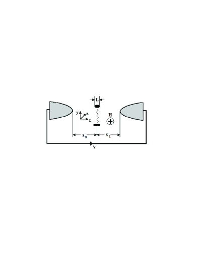
Figure 1: Schematic diagram of the device geometry. A single-level quantum ”dot” (QD) of characteristic size $L$ is placed in the gap between two point-like metal electrodes. The QD position $x_{L,R}$ on the $x$-axis is fixed and it vibrates (depicted as a spring) only along the $y$-axis. An external magnetic field is directed along the $z$-axis.

At first we calculate the tunneling current in the case when the displacement $y_{c}$ of the QD in a magnetic field (due to the Laplace force BSL ) is greater than the amplitude of zero-point fluctuations, $y_{c}\gg l_{0}$, ($l_{0}=\sqrt{\hbar/m\omega_{0}}$, $m$ is the QD mass). Then the mechanical part of the problem can be treated classically and the dependence of electrical current on magnetic field appears due to the dependence of the electron tunneling probabilities on the equilibrium position of the current-carrying QD in the magnetic field. We show that in strong magnetic fields $H$ (the appropriate limit for the considered classical problem) the current scales as $J\propto 1/H$.

In the case when the bare tunneling probabilities do not depend on the QD displacement $y_{c}$ ($y_{c}\ll x_{c}$) the magnetic field influences the current only through the phase factors (Aharonov-Bohm phase) in the tunneling Hamiltonian (this is always the case for a suspended SWNT). We considered magnetopolaronic effects in the regime of sequential electron tunneling and for resonant tunneling of polarons (polaron tunneling approximation PTA ). In these cases analytical formulae for the current were derived. We predict: (i) a Franck-Condon (polaronic) blockade of magneto-conductance in the regime of sequential electron tunneling, (ii) an anomalous temperature dependence of magneto-conductance for strong electron-vibron coupling ($\phi\simeq 1$), (iii) a magnetic field-induced narrowing of resonant conductance peaks, and (iv) an excess current at high biases, $eV\gg\hbar\omega_{0}$.

II Model Hamiltonian and equations of motion

The Hamiltonian of a single-level vibrating quantum dot in a magnetic field takes the form

$$\hat{H}=\sum_{j=L,R}(H_{j}^{(l)}+H_{j}^{(t)})+H_{D},$$ (1)

where

$$H_{j}^{(l)}=\sum_{k}(\varepsilon_{k,j}-\mu_{j})a_{k,j}^{{\dagger}}a_{k,j}$$ (2)

is the Hamiltonian of noninteracting electrons in the left ($j=L$) and right ($j=R$) leads ($\varepsilon_{kj}$ is the energy of electrons with momentum $k$, $\mu_{j}$ is the chemical potential), $a_{k,j}^{\dagger}(a_{k,j})$ are the creation (destruction) operators with the standard commutation relations $\{a_{k,j}^{\dagger},a_{q,j^{\prime}}\}=\delta_{jj^{\prime}}\delta(k-q)$. Furthermore,

$$H_{D}=\varepsilon_{0}c^{{\dagger}}c+\hbar\omega_{0}b^{{\dagger}}b$$ (3)

is the Hamiltonian of a single-level ($\varepsilon_{0}$ is the level energy) vibrating quantum dot ($\omega_{0}$ is the frequency of vibrations in the $y$- direction), $c^{{\dagger}}(c)$ and $b^{{\dagger}}(b)$ are creation (destruction) fermionic ($\{c^{{\dagger}},c\}=1$) and bosonic ($[b,b^{{\dagger}}]=1$) operators. 2005 Finally,

$$H_{j}^{(t)} = t_{j}(\hat{y})\exp(-ij\lambda_{H}\hat{y})a_{k,j}c^{\dagger}+H.c.$$ (4)

$$j = (L,R)\equiv(-,+)$$

is the tunneling Hamiltonian. Here $\hat{y}=(b^{{\dagger}}+b)\,l_{0}/\sqrt{2}$ is the coordinate operator and $\lambda_{H}=eHd/\hbar c$ is the magnetic field-induced electron-vibron coupling ShGGJ ($d$ is a parameter of dimension length; its physical meaning in our model will be clarified later). In this section, the amplitude $t_{j}(\hat{y})$ of the tunneling matrix element in Eq. (4) will be modelled by the expression

$$t_{j}(\hat{y})=t_{0j}\exp\left(-\sqrt{x_{j}^{2}+\hat{y}^{2}}/l_{t}\right),$$ (5)

where $l_{t}$ is the tunneling length and $x_{j}$ is the position of the center of mass of QD along $x$-axis, which is assumed to be fixed. We will show that our results are not sensitive to the choice of parametrization, Eq. (5).

The Heisenberg equation of motion for the fermion and boson operators are

$$i\hbar\dot{a}_{kj}=\varepsilon_{kj}a_{kj}+t_{j}^{\ast}(\hat{y})\exp(-ij\lambda_{H}\hat{y})c,$$ (6)

$$i\hbar\dot{c}=\varepsilon_{0}c+\sum_{k,j}t_{j}(\hat{y})\exp(ij\lambda_{H}\hat{y})a_{kj},$$ (7)

$$\ddot{\hat{y}}+\omega^{2}_{0}\hat{y}=m^{-1}\left(\hat{F}_{c}+\hat{F}_{L}\right),$$ (8)

where the operator expressions for the cohesive ($F_{c}$) and Laplace ($F_{L}$) forces take the form

$$\hat{F}_{c} = \sum_{k,j}\frac{\partial t_{j}(\hat{y})}{\partial\hat{y}}e^{ij\hat{\phi}}c^{\dagger}a_{kj}+H.c.,$$ (9)

$$\hat{F}_{L} = -\frac{Hd}{c}\left(\hat{I}_{L}-\hat{I}_{R}\right).$$ (10)

In the last equality in Eq. (10) we introduced the standard notation for the current operator

$$\hat{I}_{j}=\dot{N}_{j},\qquad N_{j}=\sum_{k}a_{k,j}^{\dagger}a_{k,j}.$$ (11)

At first we neglect the quantum fluctuations of the coordinate operator $\hat{y}$ and derive the equation of motion for the average (classical) coordinate $<\hat{y}>=y_{c}\gg l_{0}$. When QD vibrations are treated as classical oscillations the equations of motion for the fermion operators, Eqs. (6) and (7), become a set of first order linear differential equations, which can easily be solved analytically. After straightforward calculations (see, e.g., Ref. Fed, , where an analogous equation was derived for the electron shuttle problem) we get the following classical equation of motion (notice that we made use of the wide band approximation when calculating the averages over electron operators and introduced a coordinate-dependent level width $\Gamma_{j}(y_{c})=2\pi\nu(\varepsilon_{F})|t_{j}(y_{c})|^{2}$, where $\nu(\varepsilon_{F})$ is the electron density of states in the leads)

$$\ddot{y_{c}}+\omega^{2}_{0}y_{c}=\frac{1}{m}\left(\sum_{j}R_{j}(y_{c})\frac{\partial\Gamma_{j}(y_{c})}{\partial y_{c}}+\frac{2d}{c}J(y_{c})H\right),$$ (12)

where

$$R_{j}(y_{c})=\frac{1}{2\pi}\int_{0}^{\infty}d\varepsilon\frac{(\varepsilon-\varepsilon_{0})f_{j}(\varepsilon)}{(\varepsilon-\varepsilon_{0})^{2}+[\Gamma_{t}(y_{c})/2]^{2}}$$ (13)

and

$$J(y_{c})=\frac{e}{2\pi\hbar}\int_{0}^{\infty}d\varepsilon T_{BW}(\varepsilon;y_{c})[f_{L}(\varepsilon)-f_{R}(\varepsilon)].$$ (14)

Here $eV\gg\Gamma_{0}$ $\Gamma_{t}(y_{c})=\Gamma_{L}(y_{c})+\Gamma_{R}(y_{c})$ is the total level width, and

$$T_{BW}(\varepsilon;y_{c})=\frac{\Gamma_{L}(y_{c})\Gamma_{R}(y_{c})}{(\varepsilon-\varepsilon_{0})^{2}+[\Gamma_{t}(y_{c})/2]^{2}}$$ (15)

$$f_{j}(\varepsilon)=\left[\exp\left(\frac{\varepsilon-\mu_{j}}{T}\right)+1\right]^{-1}$$ (16)

are the Breit-Wigner transmission cofficient and Fermi-Dirac distribution function, respectively. Equation (14) is the standard Landauer-Büttiker formula for the resonant current through a single-level quantum dot. The first term on the r.h.s of Eq. (12) can be interpreted as the cohesive force, the second term coincides with the force on a current-carrying conductor in a magnetic field (Laplace force) if we identify $2d$ with the longitudinal size of the QD, $2d=L$. This is the definition of the parameter $d$. which appears in the operator form of the Aharonov-Bohm phase in the tunneling Hamiltonian, Eq. (4).

In the absence of a magnetic field, $H=0$, the equilibrium position of the transverse coordinate $y_{c}=0$. One can expect that the maximal influence of the magnetic field on the electrical current through a single-level QD occurs at high voltages, $eV\geq\Gamma_{L,R}(y_{c}=0)\equiv\Gamma_{0}^{L,R}$, that is in the regime of sequential electron tunneling. In this case Eqs. (13), (14) are strongly simplified and one finds that

$$J(y_{c})=\frac{e\Gamma(y_{c})}{\hbar},\quad\Gamma(y_{c})=\frac{\Gamma_{L}(y_{c})\Gamma_{R}(y_{c})}{\Gamma_{L}(y_{c})+\Gamma_{R}(y_{c})}$$ (17)

and ($\varepsilon_{F}$ is the Fermi energy)

$$R_{L}=R_{R}=\frac{1}{2\pi}\ln\left(\frac{eV}{2\varepsilon_{F}}\right)\qquad eV>\Gamma_{0}^{L,R}.$$ (18)

For simplification we consider symmetric junctions ($x_{L}=x_{R}=l$) for which

$$\Gamma_{L}(y_{c})=\Gamma_{R}(y_{c})=\Gamma_{0}\exp\left\{-\frac{2}{l_{t}}\left(\sqrt{l^{2}+y_{c}^{2}}-l\right)\right\},$$ (19)

where $\Gamma_{0}=2\pi\nu(\varepsilon_{F})|t_{0}|^{2}\exp(-2l/l_{t})$ is the level width of the symmetric junction in the absence of a magnetic field. According to Eq. (12) the equilibrium position of the QD in a constant magnetic field does not depend on time; in weak magnetic fields it scales linerly with $H$,

$$y_{c}(H)\simeq\frac{L}{2}\frac{H}{H_{0}}\ll l,\quad H\ll\frac{l}{L}H_{0},$$ (20)

where the characteristic magnetic field $H_{0}$ is defined by the equation

$$\frac{I_{0}H_{0}}{c}=m\omega_{R}^{2},\quad I_{0}=\frac{e\Gamma_{0}}{\hbar},$$ (21)

$$\omega_{R}^{2}=\omega_{0}^{2}+\frac{2}{\pi}\frac{\Gamma_{0}}{mll_{t}}\ln\left(\frac{2\varepsilon_{F}}{eV}\right).$$

We see from Eqs. (20) and (21) that in weak magnetic fields the only effect of the cohesive force is to renormalize the frequency $\omega_{0}$ . In tunnel junctions ($\Gamma_{0}\rightarrow 0$) the renormalization is small and can be neglected. In strong magnetic fields, $H\gg(l/L)H_{0}$, we can neglect the contribution of the cohesive force to Eq. (12) as well. The magnetic field-induced shift of the QD in this limit scales logarithmically with $H$,

$$y_{c}(H)\simeq\frac{l_{t}}{2}\ln\left\{\frac{L}{2l}\frac{H}{H_{0}}\exp\left(\frac{2l}{l_{t}}\right)\right\}\gg l.$$ (22)

In weak magnetic fields the small shift ($y_{c}\ll l$) of the QD position does not influence the tunnel current in the considered classical approach. We will see in the next section that in this case one has to take into account quantum effects (phase fluctuations in the tunnelling Hamiltonian), which strongly modify tunnel transport. In strong magnetic fields (classical limit) the current $J(H)=(e/\hbar)\Gamma(H)$ scales as $1/H$ according to Eq. (22) .

At the end of this Section we briefly comment on the influence of the magnetic field on the resonant current in the considered classical approach. In the regime of resonant electron tunneling ($T,eV\leq\Gamma_{0}$) the current depends linearly on the bias voltage $V$,

$$J_{r}(H)=4G_{0}\frac{\Gamma_{L}(H)\Gamma_{R}(H)}{[\Gamma_{L}(H)+\Gamma_{R}(H)]^{2}}V$$ (23)

($G_{0}=e^{2}/h$ is the conductance quantum). It is evident from Eq. (23) that the resonant current through a symmetric junction ($\Gamma_{L}=\Gamma_{R}$) is not affected by the magnetic field since $J_{r}(H)=J_{r}(0)=G_{0}V$. For an asymmetric junction the resonant current does not depend on magnetic field in the strong-$H$ limit when the field-induced factor in the expression for the renormalized partial widths (see Eq. (19)) is cancelled in the expression for the electrical current, Eq. (23).

III Magneto-polaronic effects.

In this section we consider the influence of quantum and thermodynamical fluctuations of the coordinate operator of QD, $\hat{y}$, on electron transport in a magnetic field. Quantum effects are significant (at low temperatures) when one can neglect the dependence of the modulus of the tunneling matrix element on the QD displacement in a magnetic field. This is always the case for tunneling through a suspended SWNT.ShGGJ

When considering the quantum effects of magnetic-field induced vibrations it is convenient to introduce the electron-vibron coupling constant in the form of a dimensionless magnetic flux, $\phi=2\pi\Phi/\Phi_{0}$ ($\Phi=HLl_{0}/2$, $\Phi_{0}=hc/e$ is the flux quantum). The dimensionless electron-vibron interaction constant $\phi$ determines the quantum phase of the tunneling matrix element

$$t_{L/R}(\hat{y})=t_{0j}\exp[\mp i\phi(b^{\dagger}+b)/\sqrt{2}],$$ (24)

where $l_{0}=\sqrt{\hbar/m\omega_{0}}$ is the amplitude of zero-point fluctuations. Resonant electron tunneling in the model Eqs. (1)-(4), (24) was studied in Ref. Pistol, using perturbation theory with respect to $\phi\ll 1$. Here we are interested in non-perturbative effects, $\phi\simeq 1$.

At first we consider the regime of sequential electron tunneling where the effects of magnetic field-induced vibrations are most pronounced. In this regime the current can be calculated perturbatively with respect to the level width $\Gamma$. The sign of the Aharonov-Bohm phase, Eq. (24), which is opposite for left- and right-tunneling electrons, does not play any role in the considered regime of tunneling (which can be treated classically by using a master equation approach). So our model is equivalent to the polaronic model of electron tunneling through a vibrating QD (see, e.g., the reviews in Refs. 2, ; 7, ). Notice that in a general case the “magnetic” problem can not be mapped to the polaronic problem because of the above mentioned “sign” difference. Pistol We show below that this difference is not essential for magneto-polaronic effects.

The average electric current $J$ in the regime of sequential electron tunneling ($k_{B}T,eV\gg\Gamma$) can be calculated by using a master equation approach. It can be represented as a sum of partial currents over “vibron channels” LM , $n>0(n<0)$, corresponding to vibron emission (absorption). Hence,

$$J(V;\phi)=J_{0}\sum_{n=-\infty}^{\infty}A_{n}(\phi)\{f_{L}(\varepsilon_{0}-n\hbar\omega_{0})-f_{R}(\varepsilon_{0}-n\hbar\omega_{0})\},$$ (25)

where $J_{0}=e\Gamma/\hbar$ is the maximal current through a single-level QD ($\Gamma=\Gamma_{L}\Gamma_{R}/(\Gamma_{L}+\Gamma_{R}$)) and the spectral weights $A_{n}$ are defined by the equation

$$\sum_{n=-\infty}^{\infty}A_{n}e^{in\omega_{0}t}=\left<e^{\pm i\phi\hat{y}(t)}e^{\mp i\phi\hat{y}(0)}\right>,$$ (26)

where the average $<...>$ is taken with respect to the Hamiltonian of noninteracting vibrons, $H_{b}=\hbar\omega_{0}b^{{\dagger}}b$. The spectral weights defined by Eq.(26) coincide with the analogous quantities in the polaronic model, where they are defined through the correlation function of operators $\exp(i\lambda\hat{p})$ ($\hat{p}$ is the momentum operator). For the equilibrated vibrons with the distribution function $n_{B}(T)=[\exp(\hbar\omega_{0}/T)-1]^{-1}$ the coefficients $A_{n}$ take the following well-known form (see, e.g., Ref. Mahan, )

$$A_{n}(\frac{\hbar\omega_{0}}{T};\phi)=\exp[-\phi^{2}(1+2n_{B})]\times$$

$$I_{n}[2\phi^{2}\sqrt{n_{B}(1+n_{B})}]\exp\left(-n\frac{\hbar\omega_{0}}{T}\right).$$ (27)

Here $I_{n}(z)$ denotes a modified Bessel function (see, e.g., Ref. RG, ). As is evident from their definition in Eq. (26), the spectral weights $A_{n}$ satisfy the sum rule

$$\sum_{n=-\infty}^{\infty}A_{n}=1,$$ (28)

which can be rewritten as a nontrivial mathematical identity for the sum of modified Bessel functions,

$$\sum_{n=-\infty}^{\infty}e^{-nx}I_{n}\left(\frac{a}{\sinh x}\right)=e^{-a\coth x},\quad a\geq 0.$$ (29)

The unitary condition Eq.(28) plays a crucial role in the derivation of analytical formulae for the current and conductance at $k_{B}T,eV\gg\hbar\omega_{0}$. Since all the analytical formulas of interest for us have already been derived in the literature on the polaronic model, we here merely formulate the results.

The magneto-conductance $G(H)$ in the regime of sequential electron tunneling takes the following asymptotics at low and high temperatures KF

$$\frac{G(H)}{G(0)}\simeq\left\{\begin{array}[]{ll}\exp(-\phi^{2}),&\Gamma\ll T\ll\hbar\omega_{0}\\ 1-\phi^{2}\frac{\hbar\omega_{0}}{2T},&T\gg\phi^{2}\hbar\omega_{0}\end{array}\right.$$ (30)

Here $G(0)=G_{0}(\pi/2)(\Gamma/T)$ is the standard formula for conductance of a single-level QD. At intermediate temperatures, $k_{B}T\sim\hbar\omega_{0}$ and for strong electron-vibron interactions, $\phi\simeq 1$, the temperature dependence of conductance is nonmonotonic (anomalous).KF This signature of polaronic effects was observed in experiments5 on electron tunneling through a carbon nanopeapod-based single-electron transistor. The asymptotics Eq. (30) coincide (up to numerical factors) with the ones found in Ref. ShGGJ, for a different model (electron tunneling through a suspended nanotube). The high temperature asymptotics in Eq. (30) exactly coincides with the corresponding quantity calculated in Ref. Pistol, for resonant electron tunneling. It is interesting to notice that the calculations based on a full quantum mechanical treatment Pistol of interacting electrons and the master equation approach yield exactly the same results in high-$T$ limit.

Now we consider the behavior of current, Eq. (25), at low temperatures as a function of bias voltage ($eV\gg\Gamma$). At $T=0$ Eq. (25) takes the form

$$J(V;\phi)=J_{0}\exp(-\phi^{2})\sum_{n=0}^{n_{m}}\frac{\phi^{2n}}{n!},$$ (31)

where $n_{m}=[eV/\hbar\omega_{0}]$ ( $[x]$ denotes the integer part of $x$). At low voltages ($eV<\hbar\omega_{0}$ ) $n_{m}=0$ and the current does not depend on $V$ and is determined by a standard formula for a saturated current through a single level QD. However, in our case the level width $\Gamma(\phi)$ is renormalized by the electron-vibron interaction,

$$J(V<\hbar\omega_{0}/e;\phi)\simeq\frac{e\Gamma(\phi)}{\hbar}=\frac{e\Gamma}{\hbar}\exp(-\phi^{2}).$$ (32)

This is the demonstration of polaronic blockade. vonOppen With an increase of bias voltage the current jumps by an amount determined by the Franck-Condon factors

$$\Delta J_{n}=J_{n+1}-J_{n}=J_{0}e^{-\phi^{2}}\frac{\phi^{2n}}{n!}$$ (33)

each time the bias voltage opens a new inelastic channel $n(V)=[eV/\hbar\omega_{0}]$, (see Fig. 2).

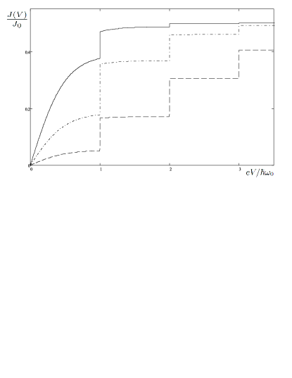
Figure 2: Low-temperature current $J(V)$ in units of $J_{0}=e\Gamma/\hbar$ as a function of bias voltage at: $\beta=\hbar\omega_{0}/T=4$, for three different values of the electron-vibron coupling constant $\phi$: the solid line corresponds to the weak- ($\phi=0.5$), the dash-dotted line to an intermediate- ($\phi=1$), and the dashed line to the strong ($\phi=1.5$) coupling regimes.

At high voltages ($eV\gg\hbar\omega_{0}$) the polaronic blockade is lifted and the current saturates at its maximum value $J_{0}$,

$$J(V\gg\hbar\omega_{0}/e;\phi)\simeq J_{0}\left\{1-e^{-\phi^{2}}\frac{\phi^{2n_{m}}}{\Gamma(n_{m}+1)}\right\}.$$ (34)

Here $\Gamma(x)$ is the gamma-function and $n_{m}=[eV/\hbar\omega_{0}]\gg\phi^{2}\gg 1$. The difference between the maximum and minimum currents

$$\delta J=J_{0}\{1-\exp(-\phi^{2})\}$$ (35)

is nothing but the excess current considered in Refs. Sonne1, ; Sonne2, for the model of electron tunneling through a suspended carbon nanotube. The presence of a high-temperature ($k_{B}T\ll eV\rightarrow\infty$) excess current in electron tunneling is another demonstration of polaronic blockade effects.

Although the magnetic field-induced polaronic effects are most pronounced in the regime of sequential electron tunneling (when the current through a single-level QD is maximal) we briefly comment here on polaronic effects in resonant electron tunneling. It is physically evident that an electron-vibron polaron state can be formed on a quantum dot coupled to reservoirs if the life-time of the electronic state, $\tau\sim\hbar/\Gamma_{t}$, is much longer than the characteristic time of polaron formation, $\tau_{p}\sim\hbar/\varepsilon_{p}\sim 1/\omega_{0}\phi^{2},(\phi\geq 1)$. The corresponding inequality $\Gamma_{t}\ll\phi^{2}\hbar\omega_{0}$ allows one to consider resonant tunneling of strongly interacting electrons in a simple model (polaron tunneling approximation PTA ). In this approximation the bare electron Green’s function (GF) in the Dyson equation for the retarded (advanced) GFs is replaced by the polaron GF ($G_{p}(\varepsilon)$)

$$G_{r,a}^{(PTA)}=\left[G_{p}^{-1}(\varepsilon)-\Sigma_{r,a}\right]^{-1},$$ (36)

where

$$G_{p}(\varepsilon)=\sum_{n=-\infty}^{\infty}\frac{A_{n}}{\varepsilon-\varepsilon_{0}+n\hbar\omega_{0}}$$ (37)

and $A_{n}$ are defined in Eq. (26). In the limit of wide electron bands in the leads the imaginary part of the self-energy function $\Sigma(\varepsilon)$ is not renormalized by electron-vibron interaction in the considered approach $\text{Im}\Sigma_{r,a}=\mp\Gamma_{t}/2$ and the real part of $\Sigma(\varepsilon)$ can be neglected. Then by evaluating the spectral function $A^{(PTA)}=i[G_{r}^{(PTA)}-G_{a}^{(PTA)}]$ one can find the current with the help of the Meir-Wingreen formula MW . It takes the form PTA

$$J=\frac{e}{\hbar}\int d\varepsilon\frac{\Gamma_{L}\Gamma_{R}G_{p}^{2}(\varepsilon)}{1+[\Gamma_{t}G_{p}(\varepsilon)/2]^{2}}\left\{f_{L}(\varepsilon)-f_{R}(\varepsilon)\right\}.$$ (38)

From Eqs. (37),(38) it is easy to show that at low temperatures ($T\ll\hbar\omega_{0}$) the conductance $G(T,\varepsilon_{0})$ in resonant tunneling can be represented in the Breit-Wigner form with the renormalized level widths $\Gamma_{L,R}(\phi)=\exp(-\phi^{2})\Gamma_{L,R}(\Gamma_{L,R}\ll\phi^{2}\hbar\omega_{0})$:

$$G(0)=G_{0}\frac{\Gamma_{L}(\phi)\Gamma_{R}(\phi)}{(\varepsilon_{F}-\varepsilon_{0})^{2}+[\Gamma_{L}(\phi)+\Gamma_{R}(\phi)]^{2}/4}.$$ (39)

According to Eq. (39) the peak conductance, $G_{r}(0,\varepsilon_{0}=\varepsilon_{F})$, is not renormalized by the magnetic field even for an asymmetric junction, $G_{r}=4G_{0}\Gamma_{L}\Gamma_{R}/[\Gamma_{L}+\Gamma_{R}]^{2}$, as is the case in the polaronic model. MAM Notice that the opposite statement, that in an asymmetric junction the peak conductance is influenced by a magnetic field Pistol , was obtained in perturbation theory with respect to the electron-vibron coupling constant $\phi\ll 1$ and that it holds in another region of model parameters, $\Gamma_{L,R}\gg\phi^{2}\hbar\omega_{0}$.

At high temperatures ($k_{B}T\gg\phi^{2}\hbar\omega_{0}$) the polaronic blockade is lifted and the formula for the conductance derived from Eq. (38) coincides with the corresponding formula (see Eq. (30)) obtained in the regime of sequential electron tunneling.

IV Conclusion.

In conclusion we have shown that the quantum-vibration-induced Aharonov-Bohm effect, predicted in Ref. ShGGJ, for electron tunneling through a suspended carbon nanotube in magnetic field, can be interpreted as a magneto-polaronic effect, where the dimensless flux $\phi=2\pi\Phi/\Phi_{0}$ plays the role of a magnetic field-induced electron-vibron interaction constant. We considered a simple model in the form of a single-level vibrating quantum “dot” (QD) in a transverse (with respect to the current flow) magnetic field - and evaluated the electrical current and the magnetoconductance in two cases: (i) the amplitude of electron tunneling depends on the magnetic field-induced QD displacement (point-like contacts), and (ii) the magnetic field influences only the Aharonov-Bohm phase of the tunneling matrix element. It was shown that magnetic field-induced polaronic effects are most pronounced: (i) in the regime of sequential electron tunneling, (ii) in high magnetic fields when the momentum $\delta p\sim eHL/c$ of the current-carrying QD induced by the Laplace force exceeds the momentum of zero-point fluctuations $p_{0}\sim\hbar/l_{0}$, and (iii) at low temperatures, $k_{B}T\ll\delta p^{2}/m$ ($m$ is the mass of the QD).

Recently polaronic effects were measured in nanotube-based single-electron transistors.3 ; 4 ; 5 In particular, a Franck-Condon blockade was observed in a suspended carbon nanotube.4 Electrically induced electron-vibron interactions happen to be much stronger than the electron-phonon interaction in isolated carbon nanotubes. So the magnetic effects could also be enhanced in the presence of ferromagnetic leads. Although simple estimations for a micron-sized nanotube-based device show that even in a very strong transverse magnetic field ($H\sim 20T$) the magnetocurrent is only of the order of 0.1 pA, the effect is measurable and its fundamental nature justifies efforts to detect it.

V Acknowledgement.

The authors thank L. Y. Gorelik and F. Pistolesi for valuable discussions. Financial support from the European Commission (FP7-ICT-FET Proj. No. 225955 STELE), the Swedish VR, the Korean WCU program funded by MEST/NFR (R31-2008-000-10057-0) and the Grant “Quantum phenomena in nanosystems and nanomaterials at low temperatures” (No. 4/10-H) from the National Academy of Sciences of Ukraine is gratefully acknowledged. I.V.K. and S.I.K. acknowledge the hospitality of the Department of Physics at the University of Gothenburg.

References

- (1) S. M. Lindsay and M. A. Ratner, Adv. Mater. 19, 23 (2007).
- (2) M. Galperin, M. A. Ratner and A. Nitzan, J. Phys. Condens. Matter 19, 103201 (2007).
-
(3)
A. K. Hüttel, M. Poot, B. Witkamp and H. S. J. van der Zant,
New J. Phys. 10, 095003 (2008);
G. A. Steele, A. K. Hüttel, B. Witkamp, M. Poot, H. B. Meerwaldt, L. P. Kouwenhoven and H. S. J. van der Zant, Science 325, 1103 (2009). - (4) R. Leturcq, Ch. Stampfer, K. Inderbitzin. L. Durrer, Ch. Hierold, E. Mariani, M. G. Schultz, F. von Oppen and K. Ensslin, Nature Physics 5, 327 (2009).
- (5) P. Utko, R. Ferone, I. V. Krive, R. I. Shekhter, M. Jonson, M. Monthioux, L. Noel and J. Nygard, Nature Communications 1, 37 (2010).
- (6) L. I. Glazman and R. I. Shekhter, Zh. Eksp. Teor. Fiz 94, 292 (1988) [Sov. Phys. JETP 67, 163 (1988)].
- (7) J. Koch and F. von Oppen, Phys. Rev. Lett. 94, 206804 (2005).
- (8) L. Y. Gorelik, A. Isacsson, M. V. Voinova, B. Kasemo, R. I. Shekhter and M. Jonson, Phys. Rev. Lett. 80, 4526 (1988).
- (9) L.M.Jonson, L.Y.Gorelik, R.I.Shekhter, M.Jonson, Nano Lett.5, 1165 (2005).
- (10) R. I. Shekhter, Yu. Galperin, L. Y. Gorelik, A. Isacsson and M. Jonson, J. Phys. Condens. Matter 15, R441 (2003).
- (11) I. V. Krive, A. Palevski, R. I. Shekhter and M. Jonson, Fiz. Nizk. Temp. 36, 155 (2010) [Low Temp. Phys. 36, 119 (2010)].
- (12) R. I. Shekhter, L. Y. Gorelik, L. I. Glazman and M. Jonson, Phys. Rev. Lett. 97, 156801 (2006).
- (13) G. Rastelli, M. Houzet and F. Pistolesi, Europhys. Lett. 89, 57003 (2010).
- (14) A. Mitra, I. Aleiner and A. J. Millis, Phys. Rev. B 69, 245302 (2004).
- (15) Each of the moving charges that contribute to the current through a conductor experiences a Lorentz force in an electromagnetic field. The Laplace force refers to the total force on the conductor.
- (16) S. Maier, T. L. Schmidt and A. Komnik, Phys. Rev. B 83, 085401 (2011).
- (17) Here we consider spinless electrons. Notice that in strong magnetic fields studied below the Zeeman splitting is so large that at all reasonable temperatures and bias voltages one can neglect the contribution of minority spin-polarized states. The effects of Zeeman splitting on electron transport in single electron transistors with spin-polirized leads were considered in: L.Y.Gorelik, S.I.Kulinich, R.I.Shekhter, M.Jonson and V.M.Vinokur, Phys. Rev. Lett. 95, 116806 (2005).
- (18) D. Fedorets, Phys. Rev. B 68, 033106 (2003).
- (19) U. Lundin and R. H. McKenzie, Phys. Rev. B 66, 075303 (2002).
- (20) G. Mahan, Many-Particle Physics, 2nd ed., Plenum Press, New York (1990).
- (21) I. S. Gradshtein and I. M. Ryzhik, Tables of Integrals, Series, and Products, Academic Press, New York and London (1965).
- (22) I. V. Krive, R. Ferone, R. I. Shekhter, M. Jonson, P. Utko and J. Nygard, New J. Phys. 10, 043043 (2008).
- (23) G. Sonne, L. Y. Gorelik, R. I. Shekhter and M. Jonson, Europhys. Lett. 84, 27002 (2008).
- (24) G. Sonne, New J. Phys. 11, 073037 (2009) .
- (25) Y. Meir and N. S. Wingreen, Phys. Rev. Lett. 68, 2512 (1992).