Efficient network-guided multi-locus association mapping with graph cuts

Abstract

As an increasing number of genome-wide association studies reveal the limitations of attempting to explain phenotypic heritability by single genetic loci, there is growing interest for associating complex phenotypes with sets of genetic loci. While several methods for multi-locus mapping have been proposed, it is often unclear how to relate the detected loci to the growing knowledge about gene pathways and networks. The few methods that take biological pathways or networks into account are either restricted to investigating a limited number of predetermined sets of loci, or do not scale to genome-wide settings.

We present SConES, a new efficient method to discover sets of genetic loci that are maximally associated with a phenotype, while being connected in an underlying network. Our approach is based on a minimum cut reformulation of the problem of selecting features under sparsity and connectivity constraints, which can be solved exactly and rapidly.

SConES outperforms state-of-the-art competitors in terms of runtime, scales to hundreds of thousands of genetic loci, and exhibits higher power in detecting causal SNPs in simulation studies than existing methods. On flowering time phenotypes and genotypes from Arabidopsis thaliana, SConES detects loci that enable accurate phenotype prediction and that are supported by the literature.

Matlab code for SConES is available at http://webdav.tuebingen.mpg.de/u/karsten/Forschung/scones/.

1 Introduction

Twin and family/pedigree studies make it possible to estimate the heritability of observed traits, that is to say the amount of their variability that can be attributed to genetic differences. In the past few years, genome-wide association studies (GWAS), in which several hundreds of thousands to millions of single nucleotide polymorphisms (SNPs) are assayed in up to thousands of individuals, have made it possible to identify hundreds of genetic variants associated with complex phenotypes (Zuk et al., 2012). Unfortunately, while studies associating single SNPs with phenotypic outcomes have become standard, they often fail to explain much of the heritability of complex traits (Manolio et al., 2009). Investigating the joint effects of multiple loci by mapping sets of genetic variants to the phenotype has the potential to help explain part of this missing heritability (Marchini et al., 2005). While efficient multiple linear regression approaches (Cho et al., 2010; Wang et al., 2011; Rakitsch et al., 2012) make the detection of such multivariate associations possible, they often remain limited in power and hard to interpret. Incorporating biological knowledge into these approaches could help boosting their power and interpretability. However, current methods are limited to predefining a reasonable number of candidate sets to investigate (Cantor et al., 2010; Fridley and Biernacka, 2011; Wu et al., 2011), for instance by relying on gene pathways. They consequently run the risk of missing biologically relevant loci that have not been included in the candidate sets. This risk is made even likelier by the incomplete state of our current biological knowledge.

For this reason, our goal here is to use prior knowledge in a more flexible way. We propose to use a biological network, defined between SNPs, to guide a multi-locus mapping approach that is both efficient to compute and biologically meaningful: We aim to find a set of SNPs that (a) are maximally associated with a given phenotype and (b) tend to be connected in a given biological network. In addition, this set must be computed efficiently on genome-wide data. In this paper we assume an additive model to characterize multi-locus association. The network constraint stems from the assumption that SNPs influencing the same phenotype are biologically linked. However, the diversity of the type of relationships that this can encompass, together with the current incompleteness of biological knowledge, makes providing a network in which all the relevant connections are present unlikely. For this reason, while we want to encourage the SNPs to form a subnetwork of the network, we also do not want to enforce that they must form a single connected component. Finally, we stress that the method must scale to networks of hundreds of thousands or millions of nodes. Approaches by Nacu et al. (2007), Chuang et al. (2007) or Li and Li (2008) developed to analyze gene networks containing hundreds of nodes do therefore not apply.

While our method can be applied to any network between genetic markers, we explore three special types of networks ( Figure 1):

• Genomic sequence network (GS): SNPs adjacent on the genomic sequence are linked together. In this setting we aim at recovering sub-sequences of the genomic sequence that correlate with the phenotype.

• Gene membership network (GM): SNPs are connected as in the sequence network described above; in addition, SNPs near the same gene are linked together as well. Usually, a SNP is considered to belong to a gene if it is either located inside said gene ore within a pre-defined distance of this gene. In this setting we aim more particularly at recovering genes that correlate with the phenotype.

• Gene interaction network (GI): SNPs are connected as in the gene membership network described above. In addition, supposing we have a gene-gene interaction network (derived, for example, from protein-protein interaction data or gene expression correlations), SNPs belonging to two genes connected in the gene network are linked together. In this setting, we aim at recovering potential pathways that explain the phenotype.

Our task is a feature selection problem in a graph-structured feature space, where the features are the SNPs and the selection criterion should be related to their association with the phenotype considered. Note that our problem is different from subgraph selection problems such as those encountered in chemoinformatics, where each object is a graph and each feature is a subgraph of its own (Tsuda, 2011).

Several approaches have already been developed for selecting graph-structured features. A number of them (Le Saux and Bunke, 2005; Jie et al., 2012) only use the graph over the features to build the learners evaluating their relevance, but do not enforce that the selected features should follow this underlying structure. Indeed they can be applied to settings where the features connectivity varies across examples, while here all individuals share the same network.

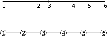
(a) Genomic sequence network: SNPs adjacent on the genomic sequence are connected to each other.

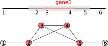
(b) Gene membership network: In addition, SNPs near the same gene (within a specified distance) are connected.

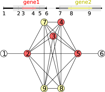
(c) Gene-interaction network: In addition, SNPs near two interacting genes are connected.

Figure 1: Small examples of the three types of networks considered.

The overlapping group Lasso (Jacob et al., 2009; Liu et al., 2012) is a sparse linear model designed to select features that belong to the union of a small number of predefined groups. If a graph over the features is given, defining those groups as all pairs of features connected by an edge or as all linear subgraphs of a given size yields the so-called graph Lasso. A similar approach is taken by Huang et al. (2009): their structured sparsity penalty encourages selecting a small number of base blocks, where blocks are sets of features defined so as to match the structure of the problem. In the case of a graph-induced structure, blocks are defined as small connected components of that graph. As shown in Mairal and Yu. (2011), the overlapping group Lasso mentioned above is a relaxation of this binary problem. As the number of linear subgraphs or connected components of a given size grows exponentially with the number of nodes of the graph, which can reach millions in the case of whole genome SNP data, only the edge-based version of the graph Lasso can be applied to our problem. It is however unclear whether it is sufficient to capture long-range connections between graph nodes.

Li and Li (2008) propose a network-constrained version of the Lasso that imposes the type of graph connectivity we deem desirable. However, their approach has been developed with networks of genes (rather than of SNPs) in mind and does not scale easily to the data sets we envision. Indeed, the implementation they propose relies on a singular value decomposition of the Laplacian of the network, which is intensive to compute and cannot be stored in memory.

Chuang et al. (2007) also searched subnetworks of protein-protein interaction networks that are maximally associated with a phenotype; however, their greedy approach requires to fix beforehand a (necessarily small) upper-limit on the size of the subnetworks considered.

In the case of directed acyclic graphs, Mairal and Yu. (2011) propose a minimum flow formulation that make it possible to use for groups (or blocks) the set of all paths of the network. Unfortunately, the generalization to undirected graphs with cycles, such as the SNP networks we consider, requires to randomly assign directions to edges and prune those in cycles without any biological justification. Although this can work reasonably well in practice (Mairal and Yu., 2011), this is akin to artificially removing more than half of the network connections without any biological justification.

In what follows, we formulate the network-guided SNP selection problem as a minimum cut problem on a graph derived from the SNP network in Section 2 and evaluate the performance of our solution both in simulations and on actual Arabidopsis thaliana data in Section 3.

2 Methods

2.1 Problem Formulation

Let $n$ be the number of SNPs and $m$ the number of individuals. The SNP-SNP network is described by its adjacency matrix ${\bm{W}}$ of size $n\times n$. A number of statistics based on covariance matrices, such as HSIC (Gretton et al., 2005) or SKAT (Wu et al., 2011), can be used to compute a measure of dependence ${\bm{c}}\in\mathbb{R}^{n}$ between each single SNP and the phenotype. Under the common assumption that the joint effect of several SNPs is additive (which corresponds to using linear kernels in those methods), ${\bm{c}}$ is such that the association between a group of SNPs and the phenotype can be quantified as the sum of the scores of the SNPs belonging to this group. That is, given an indicator vector ${\bm{f}}\in\{0,1\}^{n}$ such that, for any $p\in\{1,\cdots,n\}$, $f_{p}$ is set to $1$ if the $p$-th SNP is selected and $0$ otherwise, the score of the selected SNPs is given by $Q({\bm{f}})=\sum_{p=1}^{n}c_{p}f_{p}={\bm{c}}^{\top}{\bm{f}}$.

We want to find the indicator vector ${\bm{f}}$ that maximizes $Q({\bm{f}})$ while ensuring that the solution is made of connected components of the SNP network. However, in general, it is difficult to find a subset of SNPs that satisfies the above two properties. In fact, given a positive integer $k$, the problem of finding a connected subgraph with $k$ vertices that maximize the sum of the weights on the vertices, which is equivalent to $Q({\bm{f}})$ of our case, is known to be a strongly NP-complete problem (Lee and Dooly, 1996). Therefore, this problem is often addressed based on enumeration-based algorithms, whose runtime grows exponentially with $k$. To cope with this problem, we consider an approach based on a graph-regularization scheme, which allows us to drastically reduce the runtime.

2.2 Feature Selection with Graph Regularization

Rather than searching through all subgraphs of a given network, we reward the selection of adjacent features through graph regularization. As it is also desirable for biological interpretation and to avoid selecting large number of SNPs in linkage disequilibrium, that the selected sub-networks are small in size, we reward sparse solutions. The first requirement can be addressed by means of a smoothness regularizer on the network (Smola and Kondor, 2003; Ando and Zhang, 2007), while the second one can be enforced with an $l_{0}$ constraint:

$$\operatorname*{arg\,max}_{{\bm{f}}\in\{0,1\}^{n}}~{}\underbrace{{\bm{c}}^{\top}{\bm{f}}}_{\textrm{association}}-\underbrace{\lambda~{}{\bm{f}}^{\top}{\bm{L}}{\bm{f}}}_{\textrm{connectivity}}-\underbrace{\eta~{}\left|\left|{\bm{f}}\right|\right|_{0}}_{\textrm{sparsity}}$$ (1)

where ${\bm{L}}$ is the Laplacian of the SNP network. ${\bm{L}}$ is defined as ${\bm{L}}={\bm{D}}-{\bm{W}}$, where ${\bm{D}}$ is the diagonal matrix where ${\bm{D}}_{p,p}$ is the degree of node $p$. Note that here, we directly minimize the number of non-zero entries in $f$ and do not require the proxy of an $l_{1}$ constraint to achieve sparsity (of course in the case of binary indicators, $l_{1}$ and $l_{0}$ norms are equivalent). Positive parameters $\lambda$ and $\eta$ control the importance of the connectedness of selected features and the sparsity regularizer, respectively.

Since $W_{p,q}=1$ if $q$ is a neighbor of $p$ (also written as $p\sim q$), and $0$ otherwise, if we denote by $\mathcal{N}(p)$ the neighborhood of $p$, then the degree of $p$ can be rewritten $D_{p,p}=\sum_{q\in\mathcal{N}(p)}1$. The second term in Eq. (1) can therefore be rewritten as

$${\bm{f}}^{\top}{\bm{L}}{\bm{f}}=\sum_{p\sim q}(f_{p}-f_{q})^{2},$$ (2)

and the problem in Eq. (1) is equivalent to

$$\operatorname*{arg\,max}_{{\bm{f}}\in\{0,1\}^{n}}~{}\sum_{p=1}^{n}f_{p}(c_{p}-\eta)-\lambda\sum_{p\sim q}(f_{p}-f_{q})^{2}\;.$$ (3)

As $(f_{p}-f_{q})^{2}$ is $1$ if $f_{p}\neq f_{q}$ and $0$ otherwise, it can be seen that the connectivity term in Eq. (1) penalizes the selection of SNPs not connected to one another, as well as the selection of only subnetworks of connected components of the SNP network. Note that it does not prohibit the selection of several disconnected subnetworks. In particular, solutions may include individual SNPs fully disconnected from the other selected SNPs. Also, as $\left|\left|{\bm{f}}\right|\right|_{0}=\mathds{1}_{n}^{\top}{\bm{f}}$ in our case, the sparsity term in Eq. (1) is equivalent to reducing the individual SNP scores ${\bm{c}}$ by a constant $\eta>0$.

2.3 Min-Cut Solution

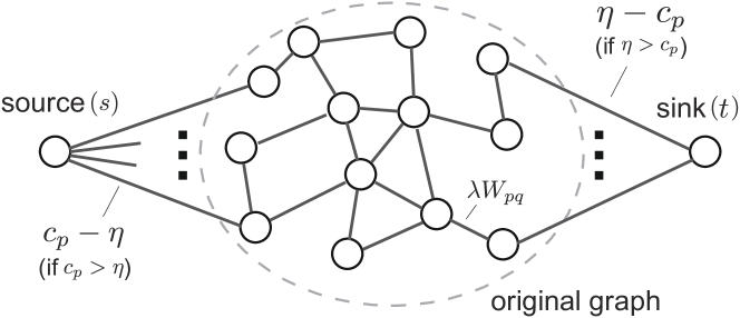
Figure 2: Graph for the $s$/$t$-min-cut formulation of the selection of networks of genetic markers.

A cut on a weighted graph over vertices $V:=\{1,\dots,n\}$ is a partition of $V$ in a non-empty set $S$ and its complementary $V\setminus S$. The cut-set of the cut is the set of edges whose end vertices belong to different sets of the partition. The minimum cut of the graph is the cut such that the sum of the weights of the edges belonging to its cut-set is minimum. If ${\bm{A}}$ is the adjacency matrix of the graph, finding the minimum cut is equivalent to finding $S\subset V$ that minimizes the cut-function $\sum_{p\in S}\sum_{q\notin S}{\bm{A}}_{p,q}=\sum_{p=1}^{n}\sum_{q=1}^{n}{\bm{f}}_{p}(1-{\bm{f}}_{q}){\bm{A}}_{p,q}$ where ${\bm{f}}_{p}$ is $1$ if $p\in S$ and $0$ otherwise. Given two vertices $s$ and $t$, an $s$/$t$-cut is a cut such that $s\in S$ and $t\in V\setminus S$. According to the max-flow min-cut theorem (Papadimitriou and Steiglitz, 1982), a minimum $s$/$t$-cut can be efficiently computed with the maximum flow algorithm (Goldberg and Tarjan, 1988).

Proposition 1

Given a graph $\mathcal{G}$ of adjacency matrix ${\bm{W}}$, solving the graph-regularized feature selection problem formalized in Eq. (1) is equivalent to finding an $s$/$t$ min-cut on the graph, depicted in Figure 2, whose vertices are that of $\mathcal{G}$, augmented by two additional nodes $s$ and $t$, and whose edges are given by the adjacency matrix ${\bm{A}}$, where ${\bm{A}}_{p,q}=\lambda{\bm{W}}_{p,q}$ for $1\leq p,q\leq n$ and

$$\begin{split}{\bm{A}}_{s,p}=\left\{\begin{array}[]{cl}c_{p}-\eta&\mbox{ if }c_{p}>\eta\\ 0&\mbox{ otherwise}\\ \end{array}\right.\text{ and }{\bm{A}}_{t,p}=\left\{\begin{array}[]{cl}\eta-c_{p}&\mbox{ if }c_{p}<\eta\\ 0&\mbox{ otherwise}\\ \end{array}\right.\\ \hfill(p=1,\ldots,n).\end{split}$$

Proof 1

The problem in Eq. (1) is equivalent to

$$\operatorname*{arg\,min}_{{\bm{f}}\in\{0,1\}^{n}}~{}(\eta\mathds{1}_{n}-{\bm{c}})^{\top}{\bm{f}}+\lambda{\bm{f}}^{\top}{\bm{L}}{\bm{f}}\,.$$ (4)

The second term of the objective is a cut-function over $\mathcal{G}$:

$${\bm{f}}^{\top}{\bm{L}}{\bm{f}}=\sum_{p=1}^{n}f_{p}\left(D_{p,p}-\sum_{q=1}^{n}W_{p,q}f_{q}\right)=\sum_{p=1}^{n}\sum_{q=1}^{n}W_{p,q}f_{p}(1-f_{q}).$$

The first term can also be encoded as a cut-function by introducing to artificial nodes $s$ and $t$:

$$\begin{array}[]{rcl}\displaystyle\sum_{p=1}^{n}(\eta-c_{p}){\bm{f}}_{p}&=&\displaystyle\sum_{\begin{subarray}{c}p\in S\\ c_{p}<\eta\end{subarray}}(\eta-c_{p})+\displaystyle\sum_{\begin{subarray}{c}p\in V\\ c_{p}\geq\eta\end{subarray}}(\eta-c_{p})-\displaystyle\sum_{\begin{subarray}{c}p\notin S\\ c_{p}\geq\eta\end{subarray}}(\eta-c_{p})\\ &=&\displaystyle\sum_{p=1}^{n}{\bm{A}}_{s,p}{\bm{f}}_{s}(1-{\bm{f}}_{p})+\displaystyle\sum_{p=1}^{n}{\bm{A}}_{p,t}{\bm{f}}_{p}(1-{\bm{f}}_{t})+\mathcal{C}\\ \end{array}$$

where $\mathcal{C}=\sum_{p\in V;c_{p}\geq\eta}(\eta-c_{p})$ is a constant, ${\bm{f}}_{s}=1$, ${\bm{f}}_{t}=0$, and ${\bm{A}}$ is defined as above. As ${\bm{f}}_{s}=1$ and ${\bm{f}}_{t}=0$ enforce that $s\in S$ and $t\notin S$, it follows that Eq. (1) is an $s$/$t$ min-cut problem on the transformed graph defined by the adjacency matrix ${\bm{A}}$ over the vertices of $\mathcal{G}$ augmented by $s$ and $t$. Note that the above still holds if ${\bm{W}}$ is a weighted adjacency matrix, and therefore the min-cut reformulation can also be applied to a weighted network. $\hfill\blacksquare$

It is therefore possible to use maximal flow algorithms to efficiently optimize the objective function defined in Equation (1) and select a small number of connected SNPs maximally associated with a phenotype. In our implementation, we use the Boykov-Kolmogorov algorithm (Boykov and Kolmogorov, 2004). Although its worst case complexity is in $\mathcal{O}(n^{2}n_{E}n_{C})$, where $n_{E}$ is the number of edges of the graph and $n_{C}$ the size of the minimum cut, it performs much better in practice, particularly when the graph is sparse. We refer to this method as SConES, for Selecting CONnected Explanatory SNPs.

3 Results

We evaluate the ability of SConES to detect networks of trait-associated SNPs on simulated datasets and on datasets from an association mapping study in Arabidopsis thaliana.

3.1 Experimental Settings

For all of our experiments, we consider the three SNP networks defined in Section 1: the genomic sequence network (GS), the gene membership network (GM), and the gene interaction network (GI). For SConES, the association term ${\bm{c}}$ is derived from Linear SKAT (Wu et al., 2011), which makes it possible to correct for covariates (and therefore population structure). SKAT has been devised to address rare variants associations problems by grouping SNPs to achieve statistical significance, but can equally be applied to common variants.

Univariate linear regression

As a baseline for comparisons, we run a linear-regression-based single-SNP search for association, and select those SNPs that are significantly associated with the phenotype (Bonferroni-corrected $p$-value $\leq 0.05$).

LMM

Similarly, we run a linear mixed model (LMM) single-SNP search for association (Lippert et al., 2011), and select those SNPs that are significantly associated with the phenotype (Bonferroni-corrected $p$-value $\leq 0.05$).

Lasso

To compare SConES to a method that also considers all additive effects of SNPs simultaneously with a sparsity constraint, but without any network regularization, we also run a Lasso regression (Tibshirani, 1994), using the SLEP implementation (Liu et al., 2009) of the Lasso.

ncLasso

In addition, we compare SConES to the network-constrained Lasso ncLasso (Li and Li, 2008), a version of the Lasso with sparsity and graph-smoothing constraints equivalent to that of SConES. Given a genotype matrix ${\bm{G}}$ and a phenotype ${\bm{r}}$, ncLasso solves the following relaxed problem (${\bm{f}}\in\mathbb{R}^{n}$):

$$\operatorname*{arg\,min}_{{\bm{f}}\in\mathbb{R}^{n}}~{}\frac{1}{2}\left|\left|{\bm{G}}{\bm{f}}-{\bm{r}}\right|\right|_{2}^{2}+\lambda{\bm{f}}^{\top}{\bm{L}}{\bm{f}}+\eta\left|\left|{\bm{f}}\right|\right|_{1}$$ (5)

The solution for ncLasso proposed by Li and Li (2008) requires to compute and store a single value decomposition of ${\bm{L}}$ and is therefore not applicable when its sizes exceeds $100\,000\times 100\,000$ by far. However, a similar solution can be obtained by decomposing ${\bm{L}}$ as the product of the network’s incidence matrix with its transpose, an approach that is much faster (particularly when the network is sparse).

groupLasso and graphLasso

Eventually, we also compare our method to the non-overlapping group Lasso (Jacob et al., 2009). The non-overlapping group Lasso solves the following relaxed problem:

$$\operatorname*{arg\,min}_{{\bm{f}}\in\mathbb{R}^{n}}~{}\frac{1}{2}\left|\left|{\bm{G}}{\bm{f}}-{\bm{r}}\right|\right|_{2}^{2}+\lambda\sum_{g\in\mathcal{G}}\left|\left|{\bm{f}}^{\mathcal{G}}\right|\right|_{2}$$ (6)

where $\mathcal{G}$ is a set of (possibly overlapping) predefined groups of SNPs. We consider the following two versions:

• graphLasso, for which the groups are directly defined from the same networks as considered for SConES as all pairs of vertices connected by an edge;

• groupLasso, for which the groups are defined sensibly as follows:

  • Genomic sequence groups (GS): pairs of adjacent SNPs (note this gives raise to the same groups as for graphLasso with the sequence network);

  • Gene membership groups (GM): SNPs near the same gene;

  • Gene interaction groups (GI): SNPs near either member of two interacting genes. Here SNPs near genes that are not in the interaction network get grouped by gene.

We use the SLEP implementation of the non-overlapping group Lasso (Liu et al., 2009), combined with the trick described by Jacob et al. (2009) to compute the overlapping group Lasso by replicating features in non-overlapping groups.

Setting the parameters

All methods considered, except for the univariate linear regression, have parameters (e.g. $\lambda$ and $\eta$ in the case of SConES) that need to be optimized. In our experiments, we run $10$-fold cross-validation grid-search experiments over ranges of values of the parameters: $7$ values of $\lambda$ and $\eta$ each for SConES and ncLasso, and $7$ values of the parameter $\lambda$ for the Lasso and the non-overlapping group Lasso (ranging from $10^{-3}$ to $10^{3}$). We then pick as optimal the parameters leading to the most stable selection, and report as finally selected the features selected in all folds. More specifically, we define stability according to a consistency index similar to that of Kuncheva (2007). Following Kuncheva (2007), the consistency index between two feature sets $S$ and $S^{\prime}$ is defined relative to the size of their overlap:

$$I_{C}(S,S^{\prime}):=\frac{\mbox{Observed}(|S\cap S^{\prime}|)-\mbox{Expected}(|S\cap S^{\prime}|)}{\mbox{Maximum}(|S\cap S^{\prime}|)-\mbox{Expected}(|S\cap S^{\prime}|)}$$

where

$$\mbox{Maximum}(|S\cap S^{\prime}|)=min(|S|,|S^{\prime}|)$$

and $\mbox{Observed}(|S\cap S^{\prime}|)$ is derived from the hypergeometric distribution as the expected probability of picking $|S^{\prime}|$ features out of $n$ such that $|S\cap S^{\prime}|$ are among the $|S|$ features in $S$:

$$P(|S\cap S^{\prime}|=r)=\frac{{|S|\choose r}{n-|S|\choose|S^{\prime}|-r}}{{n\choose|S^{\prime}|}}$$

and

$$\mbox{Expected}(|S\cap S^{\prime}|)=\mathbb{E}(P(|S\cap S^{\prime}|=r))=\frac{|S||S^{\prime}|}{n}.$$

Finally

$$I_{C}(S,S^{\prime})=\frac{n|S\cap S^{\prime}|-|S||S^{\prime}|}{n\min(|S|,|S^{\prime}|)-|S||S^{\prime}|}.$$

For an experiment with $k$ folds, the consistency is computed as the average of the $k(k-1)/2$ pairwise consistencies between sets of selected features:

$$I_{C}(S_{1},S_{2},\dots,S_{k})=\frac{k(k-1)}{2}\sum_{i=1}^{k}\sum_{j=i+1}^{k}I_{C}(S_{i},S_{j}).$$

3.2 Runtime

We first compare the CPU runtime of SConES with that of the linear regression, ncLasso and graphLasso. To assess the performance of our methods, we simulate from $100$ to $200\,000$ SNPs for $200$ individuals and generate exponential random networks with a density of $2\%$ (chosen as an upper limit on the density of currently available gene-gene interaction networks) between those SNPs.

We report the real CPU runtime of one cross-validation, for set parameters, over a single AMD Opteron CPU ($2048$KB, $2600$MHz) with $512$GB of memory, running Ubuntu 12.04 (Figure 3). Across a wide range of numbers of SNPs, SConES is at least two orders of magnitude faster than graphLasso and one order of magnitude faster than ncLasso.

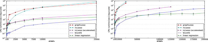
Figure 3: Real CPU runtime comparison between univariate linear regression, ncLasso, non-overlapping group Lasso and SConES, from $100$ to $25\,000$ SNPs (left) and from $100$ to $200\,000$ SNPs (right). “ncLasso” refers to the original implementation suggested by Li and Li (2008), and “ncLasso (accelerated)” to the incidence-matrix based implementation we use here. After three weeks, non-overlapping group Lasso and ncLasso had not finished running for $50\,000$ SNPs. The accelerated version of ncLasso ran out of memory for $150\,000$ SNPs or more.

3.3 Simulations

To assess the performance of our methods, we simulate phenotypes for $m=500$ real Arabidopsis thaliana genotypes ($214\,051$ SNPs), chosen at random among those made available by Horton et al. (2012), and the A. thaliana protein-protein interaction information from TAIR (The Arabidopsis Information Resource, 2012) (resulting in $55\,584\,646$ SNP-SNP connections). We use a window size of $20\,000$ base-pairs to define proximity of a SNP to a gene, in accordance with the threshold used for the interpretation of GWAS results in Atwell et al. (2010). Restricting ourselves to $1,000$ randomly picked SNPs with minor allele frequency larger than $10\%$, we pick $20$ of the SNPs to be causal, and generate phenotypes $y_{i}=w^{\top}g_{i}+\epsilon$, where both the support weights $w$ and the noise $\epsilon$ are normally distributed. We consider the following scenarios: (a) the causal SNPs are randomly distributed in the network; (b) the causal SNPs are adjacent on the genomic sequence; (c) the causal SNPs are near the same gene; (d-f) the causal SNPs are near either of two, three, and five interacting genes, respectively. We then select SNPs using univariate linear regression, Lasso, ncLasso, the two flavors of non-overlapping group Lasso, and SConES as described in Section 3.1. We repeat each experiment $30$ times, and compare the selected SNPs of either approach with the true causal ones in terms of power (fraction of causal SNPs selected) and false discovery rate (FDR, fraction of selected SNPs that are not causal). We summarize the results with F-scores (harmonic mean of power and one minus FDR) in Table 1.

As SConES returns a binary feature selection rather than a feature ranking, it is not possible to draw FDR curves or compare powers at same FDR as is often done when evaluating such methods. Figure 4 presents the average FDR and power of the different algorithms under three of the scenarios, depending on the network used. The closer the FDR-power point representing an algorithm to the upper-left corner, the better this algorithm at maximizing power while minimizing FDR. As it is easy to get better power by selecting more SNPs, we also report on the same figure the number of SNPs selected by each algorithm, and show that it remains reasonably close to the true value of $20$ causal SNPs.

SConES is systematically better than its state-of-the-art comparison partners at leveraging structural information to retrieve the connected SNPs that were causal. Only when the groups perfectly match the causal structure (Scenario (d)) can groupLasso outperform SConES. While the performance of SConES and ncLasso does depend on the network, the non-overlapping group Lasso is much more sensitive to the definition of its groups. Furthermore, we observe that removing a small fraction ($1\%$ to $15\%$) of the edges between causal features does not harm the performance of SConES (see Table 2). This means that SConES is robust to missing edges, an important point when the biological network used is likely to be incomplete. Nevertheless, the performance of SConES, as that of all other network-regularized approaches, is strongly negatively affected when the network is entirely inappropriate (Scenario (a)). In addition, the decrease in performance from Scenario (c) to Scenario (f), when the number of interacting genes near which the causal SNPs are located increases from $1$ to $5$, indicates that SConES, like its structure-regularized comparison partners, performs better when the causal SNPs are less spread out in the network. Finally, ncLasso is both slower and less performant than SConES. This indicates that solving the feature selection problem we pose directly, rather than its relaxed version, allows for better recovery of true causal features.

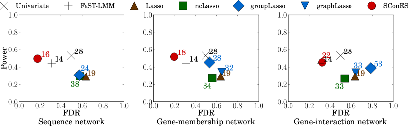
(a) Scenario (b): The true causal SNPs belong to the same genomic segment

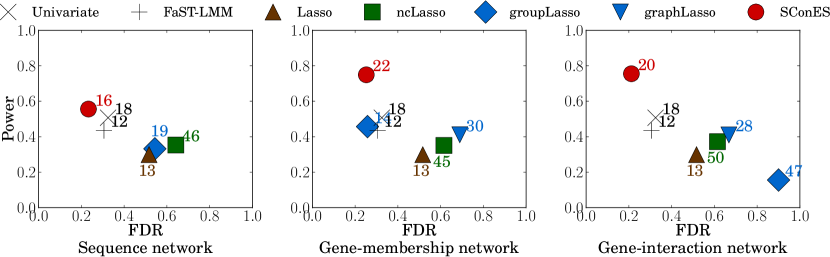
(b) Scenario (c): The true causal SNPs are near the same gene

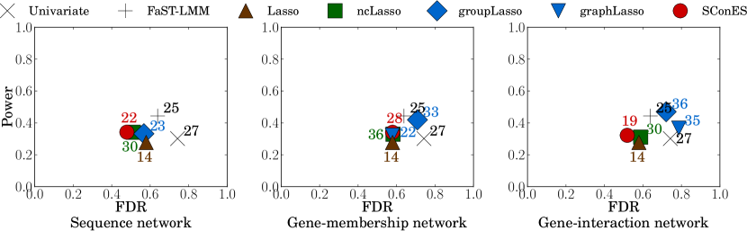
(c) Scenario (f): The true causal SNPs are near any of five interacting genes

Figure 4: Power and false discovery rate (FDR) of SConES, compared to state-of-the-art Lasso algorithms and a baseline univariate linear regression, in three different data simulation scenarios. Best methods are closest to the upper-left corner. Numbers denote the number of SNPs selected by the method.

		(a)	(b)	(c)
Univariate		$0.26\pm 0.07$	$0.29\pm 0.12$	$0.28\pm 0.14$
LMM		${\it 0.32\pm 0.01}$	$0.35\pm 0.01$	$0.33\pm 0.01$
Lasso		$\bm{0.35\pm 0.01}$	$0.32\pm 0.02$	$0.36\pm 0.01$
ncLasso	GS	$0.17\pm 0.01$	$0.25\pm 0.02$	$0.25\pm 0.01$
	GM	$0.17\pm 0.01$	$0.26\pm 0.02$	$0.26\pm 0.02$
	GI	$0.19\pm 0.01$	$0.26\pm 0.02$	$0.26\pm 0.02$
groupLasso	GS	$0.23\pm 0.01$	$0.30\pm 0.01$	$0.34\pm 0.01$
	GM	$0.12\pm 0.00$	$0.44\pm 0.02$	$0.55\pm 0.01$
	GI	$0.09\pm 0.00$	$0.26\pm 0.02$	$0.11\pm 0.01$
graphLasso	GS	$0.23\pm 0.01$	$0.30\pm 0.01$	$0.34\pm 0.01$
	GM	$0.23\pm 0.01$	$0.28\pm 0.01$	$0.33\pm 0.01$
	GI	$0.22\pm 0.01$	$0.28\pm 0.01$	$0.34\pm 0.01$
SConES	GS	$0.21\pm 0.01$	${\it 0.55\pm 0.04}$	$0.57\pm 0.04$
	GM	$0.19\pm 0.02$	$\bm{0.58\pm 0.03}$	${\it 0.75\pm 0.03}$
	GI	$0.20\pm 0.02$	$0.48\pm 0.03$	$\bm{0.78\pm 0.03}$
		(d)	(e)	(f)
Univariate		$0.27\pm 0.07$	$0.26\pm 0.07$	$0.23\pm 0.08$
LMM		$0.36\pm 0.02$	$0.38\pm 0.01$	${\it 0.33\pm 0.01}$
Lasso		$0.36\pm 0.01$	$0.37\pm 0.01$	$0.32\pm 0.01$
ncLasso	GS	$0.45\pm 0.01$	$0.38\pm 0.02$	$0.30\pm 0.01$
	GM	$0.38\pm 0.01$	$0.29\pm 0.01$	$0.27\pm 0.01$
	GI	$0.43\pm 0.02$	$0.34\pm 0.02$	$0.28\pm 0.01$
groupLasso	GS	$0.37\pm 0.01$	$0.36\pm 0.02$	$0.32\pm 0.01$
	GM	${\it 0.50\pm 0.01}$	${\it 0.40\pm 0.01}$	${\it 0.33\pm 0.01}$
	GI	$\bm{0.54\pm 0.01}$	${\it 0.40\pm 0.01}$	$\bm{0.34\pm 0.01}$
graphLasso	GS	$0.37\pm 0.01$	$0.36\pm 0.02$	$0.32\pm 0.01$
	GM	$0.36\pm 0.01$	$0.31\pm 0.01$	$0.31\pm 0.01$
	GI	$0.33\pm 0.01$	$0.30\pm 0.01$	$0.27\pm 0.01$
SConES	GS	${\it 0.50\pm 0.01}$	$\bm{0.43\pm 0.02}$	${\it 0.33\pm 0.02}$
	GM	$0.49\pm 0.01$	${\it 0.40\pm 0.02}$	$0.32\pm 0.02$
	GI	$0.49\pm 0.01$	$0.39\pm 0.01$	$\bm{0.34\pm 0.02}$

Table 1: F-scores of SConES, compared to state-of-the-art Lasso algorithms and a baseline univariate linear regression, in six different data simulation scenarios: The true causal SNPs are (a) unconnected; (b) adjacent on the genomic sequence; (c) near the same gene; (d) near either of the same $2$ connected genes; (e) near either of the same $3$ connected genes; (f) near either of the same $5$ connected genes. Best performance in bold and second best in italics. “GS”: Genomic sequence network. “GM”: Gene membership network. “GI”: Gene interaction network.

Scenario	Fraction of edges removed
	$0\%$	$2\%$	$5\%$	$10\%$	$15\%$
(b)	$0.58\pm 0.03$	$0.58\pm 0.03$	$0.58\pm 0.03$	$0.57\pm 0.03$	$0.55\pm 0.03$
(c)	$0.75\pm 0.03$	$0.75\pm 0.03$	$0.75\pm 0.03$	$0.75\pm 0.03$	$0.62\pm 0.03$
(f)	$0.34\pm 0.02$	$0.34\pm 0.02$	$0.34\pm 0.02$	$0.33\pm 0.02$	$0.29\pm 0.02$

Table 2: Effect on the F-scores of SConES of removing a small fraction of the network edges. Results reported for SConES+GM in three different scenarios: The true causal SNPs are (b) adjacent on the genomic sequence; (c) near the same gene; (f) near either of the same $5$ connected genes.

3.4 Arabidopsis Flowering Time Phenotypes

We then apply our method to a large collection of 17 A. thaliana flowering times phenotypes from Atwell et al. (2010) (up to $194$ individuals, $214\,051$ SNPs). The groups and networks are again derived from the TAIR protein-protein interaction data (The Arabidopsis Information Resource, 2012). We filter out SNPs with a minor allele frequency lower than $10\%$, as is typical in A. thaliana GWAS studies. We use the first principal components of the genotypic data as covariates to correct for population structure (Price et al., 2006): the number of principal components is chosen by adding them one by one until the genomic control is close to $1$ (see Figure 5).

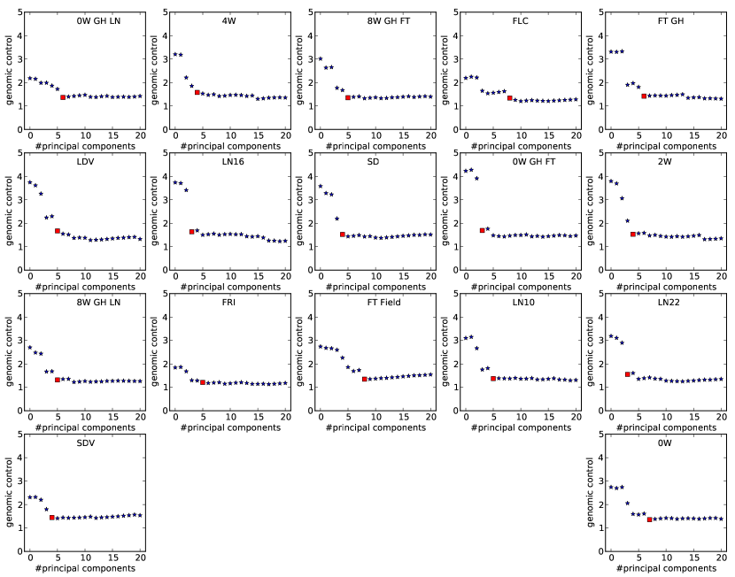
Figure 5: Genomic control values ($\lambda$) per phenotype for an increasing number of principal components (PC). The red rectangle indicates the number of PCs selected for this particular phenotype.

The direct competitors of SConES on this problem are the methods that also impose graph constraints on the SNPs they select, namely graphLasso and ncLasso. However, graphLasso does not scale to datasets such as ours with more than 200k SNPs (see Figure 3). Hence we had to exclude it from our experiments. Note that while even our accelerated implementation of ncLasso could not be run on more than $125\,000$ SNPs in our simulations, the networks derived for A. thaliana are sparser than that used in the simulations, which makes it possible to run ncLasso on this data.

Instead, we compare SConES to ncLasso and groupLasso, which uses pairs of neighboring SNPs, SNPs from the same gene or SNPs from interacting genes as pre-defined groups. Note that groupLasso on sequence-neighboring SNPs is identical to graphLasso on the sequence network, which is the only instance of graphLasso whose computation is practically feasible on this dataset. We run Lasso, ncLasso, groupLasso and SConES on the flowering time phenotypes as described in Section 3.1. However, for many of the phenotypes, the Lasso approaches select large number of SNPs (more than $10\,000$), which makes the results hard to interprete. Using cross-validated predictivity, as is generally done for Lasso, still does not entirely solve this issue, particularly for large group sizes (see Tables 5 and 6). We therefore filter out solutions containing more than $1\%$ of the total number of SNPs before using consistency to select the optimal parameters.

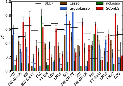
(a) Genomic sequence networks

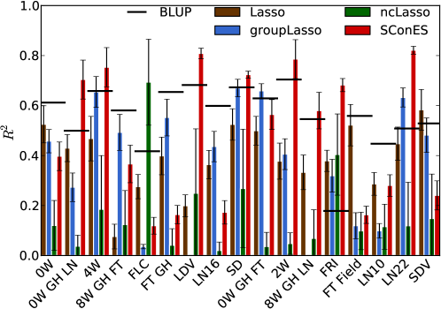
(b) Gene membership networks

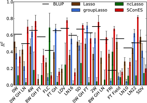
(c) Gene interaction networks

Figure 6: Cross-validated predictivity (measured as Pearson’s squared correlation coefficient between actual phenotype and phenotype predicted by a ridge-regression over the selected SNPs) of SConES compared to that of Lasso, groupLasso, and ncLasso. Horizontal bars indicate cross-validated BLUP predictivity.

To evaluate the quality of the SNPs selected, we perform ridge regression on each phenotype in a cross-validation scheme that uses only the selected SNPs and report its average Pearson’s squared correlation coefficient in Figure 6. We also report, as an additional baseline, the cross-validated predictivity of a standard best linear unbiased prediction (BLUP)  (Henderson, 1975). While the features selected by groupLasso+GS achieve higher predictivity than SConES+GS on most phenotypes, the features selected by SConES+GM are at least as predictive as those selected by groupLasso+GM in two thirds of the phenotypes; the picture is the same for SConES+GI, whose selected SNPs are on average more predictive than those of groupLasso+GI. The superiority of groupLasso in that respect is to be expected, as predicitivity is directly optimized by the regression. Also note that in $80\%$ of the cases, if any of the feature selection methods achieves high predictivity ($R^{2}>0.6$), SConES outperforms all other methods including BLUP.

Next, we checked whether the selected SNPs from the three methods coincide with flowering time genes from the literature. We report in Table 3 the number of SNPs selected by each of the methods and the proportion of these SNPs that are near flowering time candidate genes listed by Segura et al. (2012). Here, the picture is reversed: SConES+GS and groupLasso+GI retrieve the highest ratio of SNPs near candidate genes, while groupLasso+GS, SConES+GI and SConES+GM show lower ratios. At first sight, it seems surprising that the methods with highest predictive power retrieve the least SNPs near candidate genes.

To further investigate this phenomenon, we record how many distinct flowering time candidate genes are retrieved on average by the various methods. A gene is considered retrieved if the method selects a SNP near it. Our results are shown in Table 4. Methods retrieving a large fraction of SNPs near candidate genes do not necessarily retrieve the largest number of distinct candidate genes. Good predictive power, as shown in Figure 6, however, seems to correlate with the number of distinct candidate genes selected by an algorithm, not with the percentage of selected SNPs near candidate genes. groupLasso+GI has the highest fraction of candidate gene SNPs among all methods, but detects only three distinct candidate genes. This is probably due to groupLasso selecting entire genes or gene pairs; if groupLasso detects a candidate gene, it will pick most of the SNPs near that gene, which leads to its high candidate SNP ratio in Table 3.

We also compare the selected SNPs to those deemed significant by a linear mixed model ran on the full data (see Table 7). SConES systematically recovers more of those SNPs than the Lasso approaches.

To summarize, SConES is able to select SNPs that are highly predictive of the phenotype. Among all methods, SConES+GM discovers the largest number of distinct genes whose involvement in flowering time is supported by the literature.

Phenotype	Univariate	LMM	Lasso	groupLasso			ncLasso			SConES
				GS	GM	GI	GS	GM	GI	GS	GM	GI
0W	$0/3$	$0/0$	$1/29$	$33/288$	$59/706$	$144/547$	$40/1077$	$14/318$	$14/318$	$\bm{123/271}$	$0/85$	$0/69$
0W GH LN	$0/0$	$0/0$	$2/20$	$13/205$	$54/478$	$\bm{128/321}$	$31/981$	$11/320$	$11/320$	$92/1251$	$92/1252$	$92/1253$
4W	$1/8$	$1/2$	$15/129$	$7/52$	$48/1489$	$\bm{80/436}$	$2/238$	$6/298$	$6/298$	$104/1670$	$66/1078$	$42/859$
8W GH FT	$0/5$	$0/1$	$10/143$	$\bm{5/16}$	$66/1470$	$0/0$	$14/427$	$11/398$	$11/398$	$26/322$	$26/322$	$26/319$
FLC	$0/1$	$0/1$	$1/31$	$2/95$	$0/101$	$0/214$	$4/135$	$1/35$	$1/35$	$\bm{115/1592}$	$0/2$	$0/2$
FT GH	$0/1$	$2/10$	$\bm{7/46}$	$8/106$	$90/841$	$177/1417$	$37/1434$	$42/1709$	$42/1709$	$0/626$	$0/59$	$0/59$
LDV	$0/4$	$\bm{1/2}$	$10/80$	$8/32$	$0/0$	$0/0$	$14/437$	$7/177$	$7/177$	$39/674$	$86/1381$	$54/1091$
LN16	$0/5$	$0/0$	$9/222$	$0/95$	$138/957$	$89/1307$	$22/1094$	$33/1323$	$33/1323$	$\bm{73/73}$	$0/3$	$0/4$
SD	$0/2$	$0/1$	$3/36$	$36/569$	$51/863$	$84/721$	$20/466$	$10/224$	$10/224$	$\bm{7/59}$	$\bm{7/59}$	$\bm{7/59}$
0W GH FT	$0/9$	$\bm{1/3}$	$20/194$	$49/654$	$52/898$	$241/1258$	$63/1597$	$84/1997$	$84/1997$	$0/6$	$29/317$	$29/317$
2W	$0/12$	$0/6$	$4/36$	$7/79$	$93/610$	$\bm{126/810}$	$28/1006$	$43/1256$	$43/1256$	$76/756$	$78/1185$	$25/892$
8W GH LN	$0/2$	$0/3$	$8/122$	$13/168$	$0/0$	$0/0$	$19/493$	$21/501$	$21/501$	$\bm{11/73}$	$75/776$	$68/757$
FRI	$6/11$	$5/9$	$6/18$	$8/64$	$8/20$	$\bm{10/10}$	$2/9$	$2/4$	$2/4$	$101/1266$	$101/1271$	$101/1274$
FT Field	$2/4$	$0/0$	$1/79$	$5/37$	$51/221$	$\bm{52/72}$	$18/709$	$5/238$	$5/238$	$4/8$	$4/8$	$4/8$
LN10	$0/1$	$0/0$	$0/12$	$2/34$	$\bm{18/121}$	$0/202$	$12/644$	$12/649$	$12/649$	$165/1921$	$0/91$	$0/91$
LN22	$2/14$	$0/0$	$6/65$	$0/12$	$33/894$	$81/1023$	$23/501$	$26/506$	$26/506$	$\bm{140/1378}$	$\bm{140/1378}$	$140/1378$
SDV	$0/5$	$0/1$	$4/208$	$3/94$	$1/721$	$105/936$	$14/379$	$15/384$	$15/384$	$\bm{53/454}$	$0/8$	$0/8$

Table 3: Associations detected close to known candidate genes, for all flowering time phenotypes of Arabidopsis thaliana. We report the number of selected SNPs near candidate genes, followed by the total number of selected SNPs. Largest ratio in bold. “GS”: Genomic sequence network. “GM”: Gene membership network. “GI”: Gene interaction network.

	#SNPs	near candidate genes	candidate genes hit
Univariate	$5$	$0.09$	$0.35$
LMM	$2$	$0.12$	$0.35$
Lasso	$86$	$0.09$	$3.82$
groupLasso GS	$153$	$0.10$	$4.35$
groupLasso GM	$611$	$0.09$	$1.35$
groupLasso GI	$546$	$0.20$	$2.65$
ncLasso GS	$684$	$0.04$	$4.88$
ncLasso GM	$608$	$0.06$	$4.59$
ncLasso GI	$608$	$0.06$	$4.59$
SConES GS	$729$	$0.18$	$11.53$
SConES GM	$546$	$0.08$	$14.82$
SConES GI	$496$	$0.07$	$12.24$

Table 4: Summary statistics, averaged over the Arabidopsis thaliana flowering time phenotypes: average total number of selected SNPs (“#SNPs”), average proportion of selected SNPs near candidate genes (“near candidate genes”) and average number of different candidate genes recovered (“candidate genes hit”) . “GS”: Genomic sequence network. “GM”: Gene membership network. “GI”: Gene interaction network.

Phenotype	LinReg	Lasso	groupLasso			SConES
			GS	GM	GI	GS	GM	GI
0W	$3$	$53545$	$53567$	$53572$	$53816$	$271$	$85$	$69$
0W GH LN	$0$	$53759$	$53633$	$53706$	$53785$	$1251$	$1252$	$1253$
4W	$8$	$60243$	$60276$	$60354$	$60572$	$1670$	$1078$	$859$
8W GH FT	$5$	$59759$	$60426$	$59972$	$59443$	$322$	$322$	$319$
FLC	$1$	$52587$	$52491$	$52588$	$8672$	$4624$	$3115$	$2$
FT GH	$1$	$53824$	$53802$	$54024$	$54210$	$626$	$59$	$59$
LDV	$4$	$53670$	$53797$	$53600$	$7870$	$674$	$1381$	$1091$
LN16	$5$	$55308$	$55388$	$55486$	$2914$	$2113$	$3785$	$4$
SD	$2$	$54284$	$54418$	$54481$	$12664$	$59$	$59$	$59$
0W GH FT	$9$	$57189$	$57212$	$57337$	$13199$	$6$	$317$	$317$
2W	$12$	$55967$	$56062$	$56229$	$56308$	$756$	$1185$	$892$
8W GH LN	$2$	$60549$	$60520$	$60587$	$2153$	$73$	$776$	$757$
FRI	$11$	$50556$	$50631$	$50827$	$5731$	$1266$	$1271$	$1274$
FT Field	$4$	$46683$	$47122$	$221$	$47322$	$28805$	$8$	$8$
LN10	$1$	$54794$	$54967$	$54848$	$2858$	$1921$	$91$	$91$
LN22	$14$	$56537$	$56585$	$56601$	$15486$	$1378$	$1378$	$1378$
SDV	$5$	$59242$	$59368$	$59355$	$59110$	$454$	$8$	$8$

Table 5: Number of SNPs selected, for all flowering time phenotypes of Arabidopsis thaliana, when using consistency without a cardinality constraint to select parameters. “GS”: Genomic sequence network. “GM”: Gene membership network. “GI”: Gene interaction network.

Phenotype	LinReg	Lasso	groupLasso			SConES
			GS	GM	GI	GS	GM	GI
0W	$3$	$1077$	$3289$	$1827$	$17854$	$5037$	$5002$	$4968$
0W GH LN	$0$	$765$	$205$	$1796$	$19306$	$1234$	$1253$	$1253$
4W	$8$	$994$	$2902$	$8571$	$21019$	$1670$	$1910$	$1890$
8W GH FT	$5$	$1614$	$2932$	$1470$	$20347$	$322$	$322$	$281$
FLC	$1$	$1158$	$3517$	$9805$	$19905$	$5126$	$5126$	$5119$
FT GH	$1$	$197$	$591$	$2081$	$17562$	$6163$	$6161$	$6163$
LDV	$4$	$676$	$1832$	$1809$	$18329$	$2867$	$2867$	$2867$
LN16	$5$	$2319$	$5696$	$15027$	$18252$	$5824$	$6326$	$6243$
SD	$2$	$1920$	$569$	$15933$	$18655$	$59$	$59$	$59$
0W GH FT	$9$	$194$	$654$	$2514$	$20246$	$312$	$316$	$314$
2W	$12$	$135$	$387$	$11368$	$18886$	$3186$	$3001$	$3210$
8W GH LN	$2$	$1654$	$3031$	$60602$	$20109$	$816$	$827$	$826$
FRI	$11$	$1013$	$3335$	$9422$	$19281$	$1274$	$1274$	$1273$
FT Field	$4$	$1029$	$2297$	$47005$	$2242$	$8$	$7$	$7$
LN10	$1$	$607$	$184$	$1871$	$18674$	$7840$	$7846$	$7846$
LN22	$14$	$393$	$1132$	$4019$	$21308$	$1377$	$1321$	$1378$
SDV	$5$	$1860$	$10073$	$16599$	$19651$	$8757$	$4362$	$8812$

Table 6: Number of SNPs selected, for all flowering time phenotypes of Arabidopsis thaliana, when using the predictivity (cross-validated $R^{2}$ between actual phenotype and that predicted by a ridge-regression trained only on the selected SNPs) to select parameters. “GS”: Genomic sequence network. “GM”: Gene membership network. “GI”: Gene interaction network.

Phenotype	EMMA	Univariate	FaST-LMM	Lasso	groupLasso			SConES
					GS	GM	GI	GS	GM	GI
4W	$2$	$50\%$	$100\%$	$0\%$	$0\%$	$0\%$	$0\%$	$50\%$	$50\%$	$50\%$
8W GH FT	$1$	$0\%$	$100\%$	$0\%$	$0\%$	$0\%$	$0\%$	$0\%$	$0\%$	$0\%$
FLC	$1$	$0\%$	$100\%$	$0\%$	$0\%$	$0\%$	$0\%$	$0\%$	$0\%$	$0\%$
FT GH	$10$	$0\%$	$100\%$	$0\%$	$0\%$	$0\%$	$0\%$	$0\%$	$0\%$	$0\%$
LDV	$2$	$0\%$	$100\%$	$0\%$	$0\%$	$0\%$	$0\%$	$0\%$	$0\%$	$0\%$
SD	$1$	$100\%$	$100\%$	$0\%$	$0\%$	$0\%$	$0\%$	$100\%$	$100\%$	$100\%$
0W GH FT	$3$	$67\%$	$100\%$	$0\%$	$0\%$	$0\%$	$0\%$	$0\%$	$0\%$	$0\%$
2W	$6$	$33\%$	$100\%$	$0\%$	$0\%$	$0\%$	$0\%$	$17\%$	$33\%$	$17\%$
8W GH LN	$3$	$33\%$	$100\%$	$0\%$	$0\%$	$0\%$	$0\%$	$0\%$	$33\%$	$33\%$
FRI	$9$	$100\%$	$100\%$	$100\%$	$89\%$	$56\%$	$0\%$	$100\%$	$100\%$	$100\%$
SDV	$1$	$100\%$	$100\%$	$0\%$	$0\%$	$0\%$	$0\%$	$0\%$	$0\%$	$0\%$

Table 7: Fraction of SNPs deemed significantly associated with the phenotype by EMMA run the full dataset (number of such SNPs reported in the second column) that were selected. We only report the phenotypes for which EMMA returned at least one significant SNP.

4 Discussion and Conclusions

In this article, we defined SConES, a novel approach to multi-locus mapping that selects SNPs that tend to be connected in a given biological network without restricting the search to predefined sets of loci. As the optimization of SConES can be solved by maximum flow, our solution is computationally efficient and scales to whole genome data. Our experiments show that our method is one to two orders of magnitude faster than the state-of-the-art Lasso-based comparison partners, and can therefore easily scale to hundreds of thousands of SNPs. In simulations, SConES is better at leveraging the structure of the biological network to recover causal SNPs.

On real GWAS data from Arabidopsis thaliana, the predictive ability of the features selected by SConES is superior to that of groupLasso on two of the three network types we consider. When using more biological information (gene membership or interactions), SConES tends to recover more distinct explanatory genes than groupLasso, resulting in better phenotypic prediction.

The constraints imposed by groupLasso and SConES are different: while the groups given to groupLasso and the networks passed to SConES come from the same information, the groups force many more SNPs to be selected simultaneously when they may not bring much more information. This gives SConES more flexibility, and makes it less vulnerable to ill-defined groups or networks, which is especially desirable in the light of the current noisiness and incompletedness of biological networks. Our results on the genomic sequence network actually indicate that graphLasso, using pairs of network edges as groups, may achieve the same flexibility as SConES; unfortunately it is too computationally demanding to be run on the most informative networks.

We currently derive the SNP networks from neighborhood along the genome sequence, closeness to a same gene, or proximity to interacting proteins. Refining those networks and exploring other types of networks as well as understanding the effects of their topology and density is one of our next projects.

Let us note that while we do not explicitly consider linkage disequilibrium, the $l_{0}$ sparsity constraint of SConES should enforce that when several correlated SNPs are associated with a phenotype, a single one of them is picked. On the other hand, if SConES is given a genomic sequence network such as the one we describe, the graph smoothness constraint will encourage nearby SNPs to be selected together, leading to the selection of sub sequences that are likely to be haplotype blocks. Such a network should therefore only be used when the goal of the experiment is to detect consecutive sequences of associated SNPs.

For now SConES considers an additive model between genetic loci. Future work includes taking pairwise multiplicative effects into account. Replacing the association term in Equation (1) by a sum over pairs of SNPs rather than over individual SNPs results in a maximum flow problem over a fully connected network of SNPs, which cannot be solved straightforwardly, if only because the resulting adjacency matrix is too large to fit in memory on a regular computer. It might be possible, however, to leverage some of the techniques used for two-locus GWAS (Achlioptas et al., 2011; Kam-Thong et al., 2012) to help solve this problem.

Extensions of SConES to other models include the use of mixed models to account for population structure and other confounders. This is currently a challenge as it is unclear how to derive additive test statistics from such models.

An interesting extension to study would replace the Laplacian by a random-walk based matrix, derived from powers of the adjacency matrix, so as to treat differently disconnected SNPs that are closeby in the networks from those that are far apart. Although we already observe that SConES is robust to edge removal, this would likely make it more resistant to missing edges.

Another important extension of SConES is to devise a way to evaluate the statistical significance of the set of selected SNPs. Regularized feature selection approaches such as SConES or its Lasso comparison partners do not lend themselves well to the computation of $p$-values. Permutation tests could be an option, but the number of permutations to run is difficult to evaluate, as is that of hypotheses tested. Another possibility would be to implement the multiple-sample splitting approach proposed by Meinshausen et al. (2009). However, the loss of power from performing selection on only subsets of the samples is too large, given the sizes of current genomic data sets, to make this feasible. Therefore evaluating statistical significance and controlling false discovery rates of Lasso and SConES approaches alike remain a challenge for the future.

Finally, further exciting research topics include applying SConES to larger data sets from human disease consortia (we estimate it would require less than a day to run on a million of SNPs), and extending it to the detection of shared networks of markers between multiple phenotypes.

References

- Achlioptas et al. (2011) Achlioptas, P., Schölkopf, B., and Borgwardt, K. (2011). Two-locus association mapping in subquadratic time. KDD ’11, pages 726–734, New York, NY, USA. ACM.
- Ando and Zhang (2007) Ando, R. K. and Zhang, T. (2007). Learning on graph with laplacian regularization. In NIPS.
- Atwell et al. (2010) Atwell, S. et al. (2010). Genome-wide association study of 107 phenotypes in arabidopsis thaliana inbred lines. Nature, 465(7298), 627–631.
- Boykov and Kolmogorov (2004) Boykov, Y. and Kolmogorov, V. (2004). An experimental comparison of min-cut/max- flow algorithms for energy minimization in vision. IEEE T Pattern Anal, 26(9), 1124 –1137.
- Cantor et al. (2010) Cantor, R. M., Lange, K., and Sinsheimer, J. S. (2010). Prioritizing GWAS results: A review of statistical methods and recommendations for their application. Am J Hum Genet, 86(1), 6–22.
- Cho et al. (2010) Cho, S. et al. (2010). Joint identification of multiple genetic variants via elastic-net variable selection in a genome-wide association analysis. Ann. Hum. Genet., 74(5), 416–428.
- Chuang et al. (2007) Chuang, H.-Y., Lee, E., Liu, Y.-T., Lee, D., and Ideker, T. (2007). Network-based classification of breast cancer metastasis. Mol Syst Biol, 3(140).
- Fridley and Biernacka (2011) Fridley, B. L. and Biernacka, J. M. (2011). Gene set analysis of SNP data: benefits, challenges, and future directions. Eur J Hum Genet.
- Goldberg and Tarjan (1988) Goldberg, A. V. and Tarjan, R. E. (1988). A new approach to the maximum-flow problem. Journal of the ACM, 35(4), 921–940.
- Gretton et al. (2005) Gretton, A., Bousquet, O., Smola, A., and Schölkopf, B. (2005). Measuring statistical dependence with hilbert-schmidt norms. In ALT, pages 63–77. Springer-Verlag.
- Henderson (1975) Henderson, C. R. (1975). Best linear unbiased estimation and prediction under a selection model. Biometrics, 31(2), 423–447.
- Horton et al. (2012) Horton, M. W. et al. (2012). Genome-wide patterns of genetic variation in worldwide arabidopsis thaliana accessions from the RegMap panel. Nat Genet, 44(2), 212–216.
- Huang et al. (2009) Huang, J., Zhang, T., and Metaxas, D. (2009). Learning with structured sparsity. ICML ’09, page 417–424, New York, NY, USA. ACM.
- Jacob et al. (2009) Jacob, L., Obozinski, G., and Vert, J.-P. (2009). Group lasso with overlap and graph lasso. ICML ’09, pages 433–440, New York, NY, USA. ACM.
- Jie et al. (2012) Jie, B., Zhang, D., Wee, C.-Y., and Shen, D. (2012). Structural feature selection for connectivity network-based MCI diagnosis. In P.-T. Yap et al., editors, Multimodal Brain Image Analysis, volume 7509 of Lecture Notes in Computer Science, pages 175–184. Springer Berlin / Heidelberg.
- Kam-Thong et al. (2012) Kam-Thong, T. et al. (2012). GLIDE: GPU-Based Linear Regression for Detection of Epistasis. Hum Hered, 73, 220–236.
- Kuncheva (2007) Kuncheva, L. I. (2007). A stability index for feature selection. In Proceedings of the 25th IASTED International Multi-Conference: artificial intelligence and applications. ACTA Press.
- Le Saux and Bunke (2005) Le Saux, B. and Bunke, H. (2005). Feature selection for graph-based image classifiers. In J. Marques, N. Perez de la Blanca, and P. Pina, editors, Pattern Recognition and Image Analysis, volume 3523 of Lecture Notes in Computer Science, pages 147–154. Springer Berlin / Heidelberg.
- Lee and Dooly (1996) Lee, H. F. and Dooly, D. R. (1996). Algorithms for the constrained maximum-weight connected graph problem. Naval Research Logistics, 43, 985–1008.
- Li and Li (2008) Li, C. and Li, H. (2008). Network-constrained regularization and variable selection for analysis of genomic data. Bioinformatics, 24(9), 1175–1182.
- Lippert et al. (2011) Lippert, C., Listgarten, J., Liu, Y., Kadie, C. M., Davidson, R. I., and Heckerman, D. (2011). FaST linear mixed models for genome-wide association studies. Nat Meth, 8(10), 833–835.
- Liu et al. (2009) Liu, J., Ji, S., and Ye, J. (2009). SLEP: Sparse Learning with Efficient Projections. Arizona State University.
- Liu et al. (2012) Liu, J., Huang, J., Ma, S., and Wang, K. (2012). Incorporating group correlations in genome-wide association studies using smoothed group lasso. Biostatistics.
- Mairal and Yu. (2011) Mairal, J. and Yu., B. (2011). Path coding penalties for directed acyclic graphs. In Proceedings of the 4th NIPS Workshop on Optimization for Machine Learning (OPT’11).
- Manolio et al. (2009) Manolio, T. A. et al. (2009). Finding the missing heritability of complex diseases. Nature, 461(7265), 747–753.
- Marchini et al. (2005) Marchini, J., Donnelly, P., and Cardon, L. R. (2005). Genome-wide strategies for detecting multiple loci that influence complex diseases. Nat Genet, 37(4), 413–417.
- Meinshausen et al. (2009) Meinshausen, N., Meier, L., and Bühlmann, P. (2009). P-values for high-dimensional regression. J Am Stat Assoc, 104(488), 1671–1681.
- Nacu et al. (2007) Nacu, Ş., Critchley-Thorne, R., Lee, P., and Holmes, S. (2007). Gene expression network analysis and applications to immunology. Bioinformatics, 23(7), 850–858.
- Papadimitriou and Steiglitz (1982) Papadimitriou, C. H. and Steiglitz, K. (1982). Combinatorial Optimization: Algorithms and Complexity. Prentice-Hall Inc., Englewood Cliffs, NJ.
- Price et al. (2006) Price, A. L. et al. (2006). Principal components analysis corrects for stratification in genome-wide association studies. Nat Genet, 38(8), 904–909.
- Rakitsch et al. (2012) Rakitsch, B., Lippert, C., Stegle, O., and Borgwardt, K. (2012). A lasso multi-marker mixed model for association mapping with population structure correction. Bioinformatics.
- Segura et al. (2012) Segura, V. et al. (2012). An efficient multi-locus mixed-model approach for genome-wide association studies in structured populations. Nat Genet, 44(7), 825–830.
- Smola and Kondor (2003) Smola, A. and Kondor, R. (2003). Kernels and regularization on graphs. In B. Schölkopf and M. Warmuth, editors, Learning Theory and Kernel Machines, volume 2777 of Lecture Notes in Computer Science, pages 144–158. Springer Berlin / Heidelberg.
- The Arabidopsis Information Resource (2012) The Arabidopsis Information Resource (2012). TAIR Protein-Protein Interaction. http://www.arabidopsis.org/portals/proteome/proteinInteract.jsp.
- Tibshirani (1994) Tibshirani, R. (1994). Regression shrinkage and selection via the lasso. J. R. Stat. Soc. Series B, 58, 267–288.
- Tsuda (2011) Tsuda, K. (2011). Graph classification methods in chemoinformatics. In H. H.-S. Lu, B. Schölkopf, and H. Zhao, editors, Handbook of Statistical Bioinformatics, Springer Handbooks of Computational Statistics, pages 335–351. Springer Berlin Heidelberg.
- Wang et al. (2011) Wang, D., Eskridge, K., and Crossa, J. (2011). Identifying qtls and epistasis in structured plant populations using adaptive mixed lasso. J Agric Biol Environ Stat, 16, 170–184.
- Wu et al. (2011) Wu, M. C. et al. (2011). Rare-variant association testing for sequencing data with the sequence kernel association test. Am J Hum Genet, 89(1), 82–93.
- Zuk et al. (2012) Zuk, O., Hechter, E., Sunyaev, S. R., and Lander, E. S. (2012). The mystery of missing heritability: Genetic interactions create phantom heritability. P Natl Acad Sci USA, 109(4), 1193–1198.