Constructive entanglement test from triangle inequality

Abstract

We derive a simple lower bound on the geometric measure of entanglement for mixed quantum states in the case of a general multipartite system. The main ingredient of the presented derivation is the triangle inequality applied to the root infidelity distance in the space of density matrices. The obtained bound leads to entanglement criteria with a straightforward interpretation. Proposed criteria provide an experimentally accessible, powerful entanglement test.

Quantum entanglement characterizes non–classical correlations in a quantum system consisting of several subsystems Schrodinger ; Einstein ; Bengtsson ; Horodeccy ; PR_Guhne . In the case of a pure quantum state, any correlations between subsystems, that can be detected in coincidence experiments, confirm entanglement. However, in any realistic experiment one has to cope with mixed quantum states, for which the problem becomes more involved, as quantum and classical correlations may exist. To detect reliably quantum entanglement for a mixed quantum state one needs to rule out the more common case of classical correlations.

While efficient detection of quantum entanglement is not an easy task in quantum information theory, it is more difficult to characterize this phenomenon quantitatively basing on results of partial measurements that are not sufficient for full state reconstruction. Known schemes of such experimental procedure require interactions between many copies of the state investigated PH . With an interaction between two copies of the state one can estimate a lower bound on an entanglement measure mintert in terms of a two–copy entanglement witness that reproduces the difference between global and local entropy PH1 . The things become more complicated in the case of the restriction to single-copy measurements. Despite some recent progress (see Eberly ) still there is no general satisfactory answer to the question how well one can estimate given entanglement measure on the basis of noncomplete (ie. non–tomographic) experimental data.

In this work we build on a pragmatic approach advocated in AL09 ; PR_Guhne , in which one attempts to construct entanglement measures accessible in an experiment. We derive a lower bound for the geometric measure of entanglement (GME) Brody ; geometric capable to describe entanglement of an arbitrary mixed quantum state. We shall emphasize that we are unaware of any results concerning lower bounds for GME (an upper bound given in terms of the generalized robustness of entanglement can be found in Cavalcanti ). We demonstrate that our quantity can be used to compare the amount of entanglement between different mixed states of a $d\times d$ system and provides a separability test which is experimentally accessible.

Consider an arbitrary $K$–partite quantum system described in the Hilbert space $\mathcal{H}=\bigotimes_{I=1}^{K}\mathcal{H}^{I}$ with no assumption about the dimensionality of the particular subspace $\mathcal{H}^{I}$ representing the $I$-th subsystem. We denote by $\mathcal{S}_{m}$, $m=1,\ldots,K$ the set of $m$–separable pure states $\left|\phi\right\rangle_{\textrm{sep}}^{m}=\otimes_{I=1}^{m}\left|\phi_{I}\right\rangle$. We have the following chain $S_{K}\subset S_{K-1}\subset\cdots\subset S_{1}=\mathcal{H}$.

In our considerations we shall use the root infidelity distance between two mixed states $\rho_{1}$ and $\rho_{2}$ rootinfidel :

$$C_{F}\left(\rho_{1},\rho_{2}\right)=\sqrt{1-F\left(\rho_{1},\rho_{2}\right)},$$ (1)

defined with the help of the fidelity $F\left(\rho_{1},\rho_{2}\right)$. To derive our result we use the fidelity involving at least one pure state, thus we need only the restricted, simpler formula for the fidelity

$$F\left(\rho,\left|\Psi\right\rangle\left\langle\Psi\right|\right)\equiv F\left(\rho,\left|\Psi\right\rangle\right)=\left\langle\Psi\right|\rho\left|\Psi\right\rangle.$$ (2)

Finally we need to introduce the hierarchy of GME Brody ; geometric ; Cavalcanti , which in the case of pure states is defined as:

$$E_{m}\left(\left|\Psi\right\rangle\right) = 1-\max_{\left|\phi\right\rangle\in\mathcal{S}_{m}}\left|\!\left.\left\langle\phi\right|\Psi\right\rangle\right|^{2}$$

$$\equiv \min_{\left|\phi\right\rangle\in\mathcal{S}_{m}}C_{F}^{2}\left(\left|\phi\right\rangle,\left|\Psi\right\rangle\right),\quad m=2,\dots,K.$$

The second, equivalent definition follows directly from Eqs. (1, 2). The operational interpretation of the measure $E_{m}\left(\left|\Psi\right\rangle\right)$ is straightforward. If the state $\left|\Psi\right\rangle$ is $m$–separable it belongs to the set $\mathcal{S}_{m}$, thus the minimal infidelity distance is $0$, since one can always chose $\left|\phi\right\rangle\in\mathcal{S}_{m}$ to be equal $\left|\Psi\right\rangle$.

The geometric measure of entanglement for mixed states is defined geometric with the help of the convex roof construction:

$$E_{m}\left(\rho\right)=\min_{\mathcal{E}}\sum_{i}p_{i}\min_{\left|\phi\right\rangle\in\mathcal{S}_{m}}C_{F}^{2}\left(\left|\phi\right\rangle,\left|\Psi_{i}\right\rangle\right),$$ (4)

where the ensemble $\mathcal{E}=\left\{p_{i},\left|\Psi_{i}\right\rangle\right\}$ represents the mixed state $\rho$, i.e. $\rho=\sum_{i}p_{i}\left|\Psi_{i}\right\rangle\left\langle\Psi_{i}\right|$. Surprisingly, it was shown strelsov that $E_{m}\left(\rho\right)$ is simultaneously a distance measure $E_{m}\left(\rho\right)=\min_{\sigma}C_{F}^{2}\left(\sigma,\rho\right)$ with $\sigma$ being a $m$–separable mixed state, for $m=2,\dots,K$.

The lower bound on $E_{m}\left(\rho\right)$.—

Any density matrix representing a multipartite system can be characterized by its product numerical radii $L_{m}(\rho)$, often used in the theory of quantum information Gaw+10 . These quantities can be defined as the maximal expectation value of $\rho$ among normalized pure product states,

$$L_{m}\left(\rho\right)=\max_{\left|\phi\right\rangle\in\mathcal{S}_{m}}\left\langle\phi\right|\rho\left|\phi\right\rangle,\quad m=2,\dots K.$$ (5)

Note that $E_{m}\left(\left|\Psi\right\rangle\right)\equiv 1-L_{m}\left(\left|\Psi\right\rangle\right)$.

The main result of this paper is the following lower bound for the square root of the geometric measures of entanglement

$$\sqrt{E_{m}\left(\rho\right)}\geq\mathcal{R}_{m}\left(\rho\right)=\sqrt{1-L_{m}\left(\rho\right)}-\sqrt{1-\textrm{Tr}\rho^{2}}.$$ (6)

We start the derivation of (6) with an arbitrary expansion $\rho=\sum_{i}p_{i}\left|\Psi_{i}\right\rangle\left\langle\Psi_{i}\right|$ of the mixed state $\rho$. For some fixed index $i$ we chose a pure state $\left|\Psi_{i}\right\rangle$, and another pure state $\left|\phi\right\rangle$ to be specified. Since the root infidelity (1) is a legitimate metric we can write down the triangle inequality for $C_{F}\left(\left|\phi\right\rangle,\rho\right)$ with $\left|\Psi_{i}\right\rangle\left\langle\Psi_{i}\right|$ as a third state:

$$C_{F}\left(\left|\phi\right\rangle,\rho\right)\leq C_{F}\left(\left|\phi\right\rangle,\left|\Psi_{i}\right\rangle\right)+C_{F}\left(\left|\Psi_{i}\right\rangle,\rho\right).$$ (7)

If we next take the minimum with respect to $\left|\phi\right\rangle\in\mathcal{S}_{m}$ and use the definitions (1, Constructive entanglement test from triangle inequality, 5) we obtain

$$\sqrt{1-L_{m}\left(\rho\right)}\leq\sqrt{E_{m}\left(\left|\Psi_{i}\right\rangle\right)}+C_{F}\left(\left|\Psi_{i}\right\rangle,\rho\right).$$ (8)

In the next step we shall multiply the resulting inequality by $p_{i}$ and sum over $i$. The term $\sqrt{1-L_{m}\left(\rho\right)}$ is independent of $i$, while for the two terms on the right hand side we shall apply the following estimates originating from the concavity of the $\sqrt{\cdot}$ function:

$$\sum_{i}p_{i}\sqrt{E_{m}\left(\left|\Psi_{i}\right\rangle\right)}\leq\sqrt{\sum_{i}p_{i}E_{m}\left(\left|\Psi_{i}\right\rangle\right)},$$ (9)

$$\sum_{i}p_{i}C_{F}\left(\left|\Psi_{i}\right\rangle,\rho\right)\leq\sqrt{1-\sum_{i}p_{i}\left\langle\Psi_{i}\right|\rho\left|\Psi_{i}\right\rangle}.$$ (10)

In the final step we shall recognize that the sum over $i$ on the right hand side of (10) is equal to $\textrm{Tr}\rho^{2}$, so that is independent of the given ensemble $\mathcal{E}=\left\{p_{i},\left|\Psi_{i}\right\rangle\right\}$. This implies that we can immediately minimize with respect to $\mathcal{E}=\left\{p_{i},\left|\Psi_{i}\right\rangle\right\}$ producing the quantity $\sqrt{E_{m}\left(\rho\right)}$ on the right hand side of (9). Applying the above estimates to Eq. (8) we obtain the desired lower bound (6) after a one–step rearrangement. From (6) one can obviously find the lower bound for $E_{m}\left(\rho\right)$, which reads $\left(\max\left[\mathcal{R}_{m}\left(\rho\right);0\right]\right)^{2}$. It is important to take the maximum first, in order to avoid cases when negative values of $\mathcal{R}_{m}\left(\rho\right)$ can give a positive, unphysical contribution $\mathcal{R}_{m}^{2}\left(\rho\right)$ to the lower bound of $E_{m}\left(\rho\right)$.

We shall further observe that the quantity $1-L_{m}\left(\rho\right)$ provides a natural (but typically rough) upper bound for $E_{m}\left(\rho\right)$, To prove this statement it is sufficient to restrict the minimization in $E_{m}\left(\rho\right)=\min_{\sigma}C_{F}^{2}\left(\sigma,\rho\right)$ to pure states $\sigma=\left|\phi\right\rangle\left\langle\phi\right|$. This upper bound, as well as our lower bound are in the case of pure states equal to $E_{m}\left(\rho\right)$. In the case of pseudo–pure states characterized by $\textrm{Tr}\rho^{2}\lesssim 1$ we thus get a sharp estimate of the value of the entanglement measure in question.

Let us now focus on the family of generalized $d\times d$ Werner states ($0\leq p\leq 1$):

$$\rho_{p,\boldsymbol{\lambda}}=\left(1-p\right)\left|\Psi_{\boldsymbol{\lambda}}\right\rangle\left\langle\Psi_{\boldsymbol{\lambda}}\right|+p\frac{I_{d}\otimes I_{d}}{d^{2}},$$ (11)

where $\left|\Psi_{\boldsymbol{\lambda}}\right\rangle=\sum_{i=1}^{d}\sqrt{\lambda_{i}}\left|ii\right\rangle$. One can straightforwardly calculate (as $\rho_{p,\boldsymbol{\lambda}}$ is bipartite we can skip the index $m$):

$$\textrm{Tr}\rho_{p,\boldsymbol{\lambda}}^{2}=1+\frac{\left(p^{2}\!-\!2p\right)\left(d^{2}\!-\!1\right)}{d^{2}},\;\;L\left(\rho_{p,\boldsymbol{\lambda}}\right)=\frac{p}{d^{2}}+\left(1-p\right)\Lambda,$$ (12)

where $\Lambda=\max_{i}\lambda_{i}$ and $1/d\leq\Lambda\leq 1$. The above family possesses a distinguished member given by $\boldsymbol{\bar{\lambda}}=\left(1/d,\ldots,1/d\right)$, which for $p=0$ represents the maximally entangled state. Comparing $E\left(\rho_{p,\boldsymbol{\bar{\lambda}}}\right)$ with the lower bound based on $\mathcal{R}\left(\rho_{p^{\prime},\boldsymbol{\lambda}}\right)$ for $p^{\prime}<p$ and vector $\boldsymbol{\lambda}$ majorizing MO79 $\boldsymbol{\bar{\lambda}}$ we can look for the states $\rho_{p^{\prime},\boldsymbol{\lambda}}$ which are more entangled than $\rho_{p,\boldsymbol{\bar{\lambda}}}$ (see Fig. 1 and Supplement ).

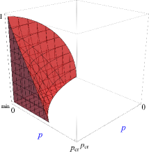
Figure 1: (color online). Parameter space for the generalized Werner states of a $3\times 3$ system. Red volume corresponds to the states $\rho_{p^{\prime},\boldsymbol{\lambda}}$ the entanglement of which is shown by the bound (6) to be larger than this of reference state $\rho_{p,\boldsymbol{\bar{\lambda}}}$. Here $d=3$ so that $p_{\textrm{cr}}=3/4$ and $\Lambda_{\textrm{min}}=1/3$.

Entanglement criteria.—

Eq. (6) provides the entanglement criteria

$$\left(L_{m}\left(\rho\right)<\textrm{Tr}\rho^{2}\right)\;\Rightarrow\;\left(\rho\textrm{ is not m--separable}\right),$$ (13)

which for $m=K$ have been recently recognized in GSarbicki ; Badziag . In GSarbicki they appear in the form of a nonlinear entanglement witness $L_{K}\left(\rho\right){\rm 1l}-\rho$, while in Badziag a more general object (see Eq. (12) from Badziag ) that contains $L_{K}\left(\rho\right)$ as a special case has been introduced. The above situation is similar to the case of purity–entropy entanglement criteria pur/ent given in terms of the Rényi entropy $H_{\alpha}$, which for $\alpha=2$ was shown mintert to establish the lower bound for the concurrence concurence . Let us emphasize in passing that the criteria (13) are strong enough to detect bound entanglement Supplement of a concrete family Bound-activation .

Let us now study the entanglement criteria (13) in the case of a bipartite $M\times N$ system. A general mixed state of such system can be written as

$$\rho = \frac{1}{MN}\left[I_{M}\otimes I_{N}+k_{M}\sum_{i=1}^{M^{2}-1}q_{i}\sigma_{i}\otimes I_{N}\right.$$

$$+ \left.k_{N}\sum_{j=1}^{N^{2}-1}p_{j}I_{M}\otimes\tilde{\sigma}_{j}+k_{M}k_{N}\sum_{i=1}^{M^{2}-1}\sum_{j=1}^{N^{2}-1}B_{ij}\sigma_{i}\otimes\tilde{\sigma}_{j}\right],$$

where $\sigma_{i}$, $i=1,\ldots,M^{2}-1$ and $\tilde{\sigma}_{j}$, $j=1,\ldots,N^{2}-1$ are traceless, hermitian generators of $SU\left(M\right)$ and $SU\left(N\right)$ groups respectively, normalized such that $\textrm{Tr}\sigma_{i}\sigma_{i^{\prime}}=2\delta_{i^{\prime}i}$ and $\textrm{Tr}\tilde{\sigma}_{j}\tilde{\sigma}_{j^{\prime}}=2\delta_{j^{\prime}j}$. For further convenience we set $k_{M}=\sqrt{MM_{-}/2}$ where $M_{-}=M-1$ and similarly for $k_{N}$. In the above representation the state is described by two Bloch vectors $\boldsymbol{p}$, $\boldsymbol{q}$ of the partially reduced states and the $\left(M^{2}-1\right)\times\left(N^{2}-1\right)$ correlation tensor $\mathbf{B}$ Bengtsson . Let us recall that the Bloch vector $\boldsymbol{q}$ belongs to the space $\mathcal{B}\left(M\right)$ defined by the constraints $\boldsymbol{q}\cdot\boldsymbol{q}=1$ and $2\left(M-2\right)\boldsymbol{q}=k_{M}\textrm{Tr}\left(\left(\boldsymbol{q}\cdot\boldsymbol{\sigma}\right)^{2}\boldsymbol{\sigma}\right)$ Bloch1 ; Bloch2 , and an equivalent definition holds for $\boldsymbol{p}\in\mathcal{B}\left(N\right)$.

The pure separable state $\left|\phi\right\rangle\left\langle\phi\right|$ present in (5) can be completely characterized by a couple of Bloch vectors $\boldsymbol{v}\in\mathcal{B}\left(M\right)$ and $\boldsymbol{w}\in\mathcal{B}\left(N\right)$. In that representation the product numerical radius $L\left(\rho\right)$ reads

$$\frac{1+\max_{\boldsymbol{v},\boldsymbol{w}}\left(M_{-}\boldsymbol{v}\!\cdot\boldsymbol{q}+N_{-}\boldsymbol{w}\!\cdot\boldsymbol{p}+M_{-}N_{-}\boldsymbol{v}\!\cdot\!\mathbf{B}\boldsymbol{w}\right)}{MN}.$$ (15)

The above maximization over $\left(\boldsymbol{v},\boldsymbol{w}\right)\in\mathcal{B}\left(M\right)\times\mathcal{B}\left(N\right)$ can be efficiently performed numerically even for larger systems, eg. $M,N=10$. To get however a deeper insight we provide in the Supplemental Material Supplement the following upper bound for (15):

$$L\left(\rho\right)\leq\frac{1+N_{-}\left\|\boldsymbol{p}\right\|+M_{-}\left\|\boldsymbol{q}\right\|+M_{-}N_{-}\sqrt{\xi_{1}\left(\mathbf{C}\right)}}{MN},$$ (16)

where $\xi_{1}\left(\mathbf{C}\right)$ denotes the largest eigenvalue of $\mathbf{C}=\mathbf{B}^{T}\mathbf{B}$ or $\mathbf{C}=\mathbf{B}\mathbf{B}^{T}$ (both quadratic matrices $\mathbf{B}^{T}\mathbf{B}$ and $\mathbf{B}\mathbf{B}^{T}$ possess the same trace and nonzero eigenvalues). The purity of $\rho$ can also be easily computed:

$$\textrm{Tr}\rho^{2}=\frac{1+N_{-}\left\|\boldsymbol{p}\right\|^{2}+M_{-}\left\|\boldsymbol{q}\right\|^{2}+M_{-}N_{-}\textrm{Tr}\mathbf{C}}{MN}.$$ (17)

In fact, if any upper bound on $L_{m}\left(\rho\right)$ is smaller than $\textrm{Tr}\rho^{2}$ then the condition (13) is satisfied. In the above case our entanglement test can thus be rewritten as: If

$$M_{-}\left\|\boldsymbol{q}\right\|\left(1-\left\|\boldsymbol{q}\right\|\right)+N_{-}\left\|\boldsymbol{p}\right\|\left(1-\left\|\boldsymbol{p}\right\|\right)+M_{-}N_{-}f\left(\mathbf{C}\right)<0,$$ (18)

where $f\left(\mathbf{C}\right)=\sqrt{\xi_{1}\left(\mathbf{C}\right)}-\textrm{Tr}\mathbf{C}$, then the mixed state $\rho$ is entangled. Note that the above criterion is invariant under local unitary operations $U_{A}\otimes U_{B}$ what follows from the fact that a unitary rotation $UXU^{\dagger}$ of any matrix $X$ is an isometry in the Hilbert-Schmidt space. This means that for a given state $\rho_{AB}$ entanglement of its all $U_{A}\otimes U_{B}$ transformations is detected with the same efficiency.

In order to investigate the performance of the new criteria (18) we shall use the state $\rho_{p,\lambda}\equiv\rho_{p,\boldsymbol{\lambda}}$ given by Eq. (11) with $d=2$, so that $\boldsymbol{\lambda}=\left(\lambda,1-\lambda\right)$. This state is described by $\boldsymbol{p}=\boldsymbol{q}=\left(0,0,z\right)$, with $z=\left(1-p\right)\left(2\lambda-1\right)$, and $\mathbf{B}=\left(1-p\right)\textrm{diag}\left(\eta,\eta,1\right)$ with $\eta=2\sqrt{\lambda\left(1-\lambda\right)}$. By a direct substitution and comparison with (12) one can check that the bound (16) becomes tight.

From the PPT criteria we know that $\rho_{p,\lambda}$ is separable when $p\geq 1-\left(1+2\eta\right)^{-1}$. In the maximally entangled case $\lambda=1/2$ the threshold for separability is thus $p_{\textrm{sep}}=2/3$. According to the criteria (18) the state $\rho_{p,\lambda}$ is entangled for $p\leq 4\left(1-\max\left[\lambda;1-\lambda\right]\right)/3$. Note that for $\lambda=1/2$ we obtain the separability threshold $p=2/3$, so that a full range of entangled Werner states is detected. This conclusion remains valid for an arbitrary dimension $d$, where deVic $\boldsymbol{p}=0=\boldsymbol{q}$ and $\mathbf{C}$ is the identity matrix multiplied by $\left(1-p\right)^{2}/\left(d-1\right)^{2}$.

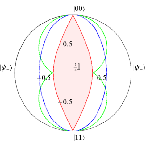
Figure 2: (color online). The plane of a family of two–qubit states $\rho_{p,\lambda}$ (points inside gray circle) in the polar coordinate $r=1-p$, $\theta=2\arccos\sqrt{\lambda}$ . States in the shaded region bounded by solid red curve are separable (PPT). Entangled states outside dashed green curve and outside dotted blue curve are detected by the criteria (18) and the purity test respectively.

In Fig. 2 we compare the criteria (18) (dashed green curve) and the purity–entropy test pur/ent (dotted blue curve) given by the condition $\textrm{Tr}\rho_{A/B}^{2}\geq\textrm{Tr}\rho^{2}$ satisfied when $\rho$ is separable. Here $\rho_{A/B}$ denote density operators of single subsystem $A$ and $B$ respectively. In the neighborhood of the maximally entangled state ($\lambda=1/2$) the criteria (13) outperform the purity test.

The above criteria has somehow built in the purity requirement but, as we have seen above, its power does not necessarily depend on how pure the state is. It might however be sensitive to the degree of purity of the element in the mixture that is responsible for entanglement. To study this possibility we check the family of $U\otimes U$ invariant $d\otimes d$ original Werner states Werner89 . This family is defined by $\rho(\alpha,d)=\left(I_{d}\otimes I_{d}+\alpha V\right)/\left(d^{2}+\alpha d\right)$ with the swap operator $V$, a real parameter $\alpha\in[-1,1]$ and sharp entanglement condition $\alpha\in[-1,-1/d)$ following from PPT test. The states are known to have $\boldsymbol{p}=0=\boldsymbol{q}$, what can be seen immediately by considering their partial transpose. With the help of formula $\textrm{Tr}(A_{1}\otimes A_{2}V)=\textrm{Tr}(A_{1}A_{2})$ Werner89 the matrix $\mathbf{B}=\alpha dI_{d}/(d^{2}+\alpha d)(d-1)$ can be easily found. The condition (18) reports entanglement for $\alpha\in[-1,-\frac{d}{d+2})$ converging to the single-point extreme $\alpha=-1$ rather than the entanglement-corresponding interval $[-1,-1/d)$ with $d\rightarrow\infty$. Using Eq. (15) we see however that

$$(d-1)^{2}\max_{\boldsymbol{v},\boldsymbol{w}}\boldsymbol{v}\cdot\mathbf{B}\boldsymbol{w}=\frac{\alpha\left(d-1\right)}{d+\alpha}\max_{\boldsymbol{v},\boldsymbol{w}}\boldsymbol{v}\cdot\boldsymbol{w}=-\frac{\alpha}{d+\alpha},$$ (19)

provided that $\alpha<0$. The last equality appears since if $\boldsymbol{v},\boldsymbol{w}\in\mathcal{B}\left(d\right)$ then $-1/(d-1)\leq\boldsymbol{v}\cdot\boldsymbol{w}\leq 1$ Bloch1 . With the above result we recover the entanglement condition $\alpha<-1/d$.

Experimental advantages.—

The entanglement test (18) can be successfully used provided that $\boldsymbol{p}$, $\boldsymbol{q}$ and $\mathbf{C}$ are known. In fact, in order to determine $\xi_{1}\left(\mathbf{C}\right)$ all matrix elements of the positive, symmetric matrix $\mathbf{C}$ must be found, what in principle requires quantum tomography. In the two–qubit case, our criteria while faithful on the family of Werner states, will always be less practical than the PPT condition. Our aim is thus to reduce the number of necessary parameters. To this end we shall upper bound the function $f\left(\mathbf{C}\right)$, so that the upper bound $g\left(\mathbf{C}\right)\geq f\left(\mathbf{C}\right)$ depends on less number of matrix entries. If inequality (18) is satisfied with $f\left(\mathbf{C}\right)$ substituted by $g\left(\mathbf{C}\right)$ then the state in question is obviously entangled. In order to achieve this goal we shall distinguish the matrix elements of $\mathbf{C}$ to be measured and maximize $f\left(\mathbf{C}\right)$ with respect to the remaining parameters. Performing the maximization we shall preserve the positivity of $\mathbf{C}$.

Let us explain the above approach using an example of two qubits, so that $\mathbf{C}$ is a real, symmetric, $3\times 3$ matrix given by six parameters: $C_{11}$, $C_{12}$, $C_{22}$, $C_{13}$, $C_{23}$, $C_{33}$. Assume that we would like to measure $C_{11}$, $C_{12}$, $C_{22}$ and optimize $f\left(\mathbf{C}\right)$ with respect to $C_{13}$, $C_{23}$, $C_{33}$. We obtain:

$$f\left(\mathbf{C}\right)\leq g\left(C_{11},C_{12},C_{22}\right)\equiv\max_{C_{13},C_{23},C_{33}}f\left(\mathbf{C}\right).$$ (20)

For the two–qubit Werner state we have: $C_{11}=\left(1-p\right)^{2}=C_{22}$, $C_{12}=0$, so that the condition for $\mathbf{C}$ to be positive reads:

$$C_{13}^{2}+C_{23}^{2}\leq C_{33}\left(1-p\right)^{2}.$$ (21)

After analytical optimization Supplement we find $g\left(C_{11},C_{12},C_{22}\right)\equiv g\left(p\right)$ of the form:

$$g\left(p\right)=\begin{cases}\left(1-p\right)\left(2p-1\right)&\qquad\textrm{for }0\leq p\leq\frac{1}{2}\\ \frac{1}{4}-\left(1-p\right)^{2}&\qquad\textrm{for }\frac{1}{2}\leq p\leq 1\end{cases}.$$ (22)

According to the test (18) the Werner state is detected to be entangled if $g\left(p\right)<0$, so that for $p<1/2$. This is up to now the best known threshold value for entanglement verification of the family of the Werner states, obtained without resorting to quantum tomography. Let us remind that the threshold value given by the purity test is $p=1-1/\sqrt{3}\approx 0.4226$.

In fact, $10$ parameters suffice (see the Supplemental Material Supplement for explicit relations between the desired and measured parameters) to determine $\left\|\boldsymbol{p}\right\|$, $\left\|\boldsymbol{q}\right\|$ and $C_{11}$, $C_{12}$, $C_{22}$. It is once again a huge experimental advantage, as in order to measure the global purity $\textrm{Tr}\rho^{2}$ of a two–qubit state one needs $12$ parameters. This improvement could be obtained because of the interplay between the purity $\textrm{Tr}\rho^{2}$ and the product numerical radius $L\left(\rho\right)$.

At the end let us analyze the $K$–qubit state

$$\varrho(p)=\left(1-p\right)\left|\Phi_{K}\right\rangle\left\langle\Phi_{K}\right|+\frac{p}{2^{K}}I^{\otimes K},$$ (23)

where $\left|\Phi_{K}\right\rangle=\left(\left|0\right\rangle^{\otimes K}+\left|1\right\rangle^{\otimes K}\right)/\sqrt{2}$. The high symmetry of the above state provides that $L_{m}\left(\varrho\right)=\left(1-p\right)/2+p/2^{K}$ for all $m\in\left\{2,\ldots,K\right\}$, what implies that all bounds $R_{m}\left(\varrho\right)$ capture the genuine multipartite entanglement of $\varrho$ associated with $m=2$. In fact, $R_{m}\left(\varrho\right)=0$ leads to the biseparability threshold $p_{\textrm{gme}}=1/2\left(1-2^{-K}\right)$, which according to Seev is optimal.

I Entanglement ordering

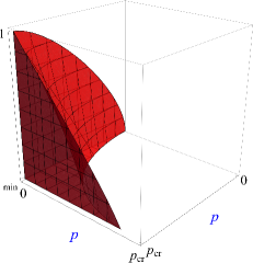
Figure 3: Parameter space for the generalized Werner states of a $10\times 10$ system. Red volume corresponds to the states $\rho_{p^{\prime},\boldsymbol{\lambda}}$ the entanglement of which is shown by our bound to be larger than this of reference state $\rho_{p,\boldsymbol{\bar{\lambda}}}$. Here $d=10$ so that $p_{\textrm{cr}}=10/11$ and $\Lambda_{\textrm{min}}=1/10$.

In geometric it was shown that for the state $\rho_{p,\boldsymbol{\bar{\lambda}}}$ one can find the exact formula for the geometric measure of entanglement (GME):

$$E\left(\rho_{p,\boldsymbol{\bar{\lambda}}}\right)=1-\frac{1}{d}\left(\mathcal{\sqrt{F}}+\sqrt{\left(d-1\right)\left(1-\mathcal{F}\right)}\right)^{2},$$ (24)

where

$$\mathcal{F}=1-\frac{p\left(d^{2}-1\right)}{d^{2}}.$$ (25)

Using Eq. (12) of our paper we can find that

$$\mathcal{R}\left(\rho_{p^{\prime},\boldsymbol{\lambda}}\right)=\sqrt{1-\frac{p^{\prime}}{d^{2}}-\left(1-p^{\prime}\right)\Lambda}-\frac{\sqrt{\left(2p^{\prime}\!-\!\left(p^{\prime}\right)^{2}\right)\left(d^{2}\!-\!1\right)}}{d}.$$ (26)

The relation $\mathcal{R}\left(\rho_{p^{\prime},\boldsymbol{\lambda}}\right)>E\left(\rho_{p,\boldsymbol{\bar{\lambda}}}\right)$ is a sufficient condition for $\rho_{p^{\prime},\boldsymbol{\lambda}}$ to be more entangled than $\rho_{p,\boldsymbol{\bar{\lambda}}}$, which is considered to be our reference state.

In the main paper we present the first nontrivial case of $d=3$. The volume of states found by our lower bound for $d=10$ is shown in Fig. 3.

II Bound entanglement

Consider now an example of the two–qutrit state Bound-activation :

$$\rho_{\alpha}=\frac{2}{7}\left|\Psi_{+}\right\rangle\left\langle\Psi_{+}\right|+\frac{\alpha}{21}\sigma_{+}+\frac{5-\alpha}{21}\sigma_{-},$$ (27)

where

$$\left|\Psi_{+}\right\rangle=\left(\left|00\right\rangle+\left|11\right\rangle+\left|22\right\rangle\right)/\sqrt{3},$$ (28)

is now a two–qutrit maximally entangled state and

$$\sigma_{+}=\textrm{diag}\left(0,1,0,0,0,1,1,0,0\right),$$ (29)

$$\sigma_{-}=\textrm{diag}\left(0,0,1,1,0,0,0,1,0\right).$$ (30)

For $2\leq\alpha\leq 3$ the state $\rho_{\alpha}$ is separable, for $3<\alpha\leq 4$, it is entangled but PPT (bound entangled), while for $4<\alpha\leq 5$ the state is entangled and not PPT.

A straightforward calculation yields

$$\textrm{Tr}\rho_{\alpha}^{2}=\frac{37+2\alpha\left(\alpha-5\right)}{147}.$$ (31)

The product numerical radius is given by the formula Gaw+10

$$L\left(\rho\right)=\max_{\left|\psi\right\rangle,\left|\chi\right\rangle}\left\langle\chi\right|\otimes\left\langle\psi\right|\rho\left|\chi\right\rangle\otimes\left|\psi\right\rangle,$$ (32)

where the maximum is taken over the set of normalized states $\left\langle\psi\left|\psi\right\rangle\right.=1$ and $\left\langle\chi\left|\chi\right\rangle\right.=1$. In order to find $L\left(\rho_{\alpha}\right)$ we parametrize $\left|\psi\right\rangle=a\left|0\right\rangle+b\left|1\right\rangle+c\left|2\right\rangle$, with the constraint $\left|a\right|^{2}+\left|b\right|^{2}+\left|c\right|^{2}=1$ and find:

$$L\left(\rho_{\alpha}\right) = \max_{\left|\chi\right\rangle}\left\langle\chi\right|\left[\frac{2}{21}\left|\psi\right\rangle\left\langle\psi\right|+\frac{\alpha}{21}\textrm{diag}\left(\left|b\right|^{2},\left|c\right|^{2},\left|a\right|^{2}\right)\right.$$ (33)

$$+ \left.\frac{5-\alpha}{21}\textrm{diag}\left(\left|c\right|^{2},\left|a\right|^{2},\left|b\right|^{2}\right)\right]\left|\chi\right\rangle.$$

The maximization with respect to $\left|\chi\right\rangle$ gives the largest eigenvalue of the $3\times 3$ matrix suited between $\left\langle\chi\right|\ldots\left|\chi\right\rangle$. This eigenvalue depends only on the moduli: $\left|a\right|$, $\left|b\right|$ and $\left|c\right|$, thus due to the normalization condition it is a complicated, two–variable function. This function attains its maximum for:

$$\begin{cases}\left|a\right|=\left|b\right|=\left|c\right|=1/\sqrt{3}&\quad\textrm{for }\alpha\leq 11/3\\ \left|a\right|=1\;\vee\;\left|b\right|=1\;\vee\;\left|c\right|=1&\quad\textrm{for }\alpha\geq 11/3\end{cases}.$$ (34)

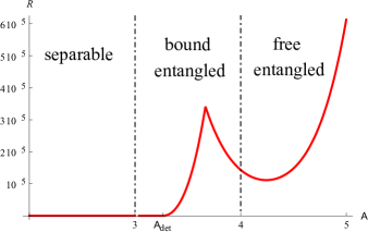
Figure 4: The lower bound for $E\left(\rho_{\alpha}\right)$ as a function of $\alpha$. Positive values implies entanglement (bound entanglement for $\alpha\leq 4$).

Plugging the values of optimizing parameters we obtain the product numerical radius:

$$L\left(\rho_{\alpha}\right)=\frac{1}{21}\max\left[\frac{11}{3};\alpha\right].$$ (35)

According to our method we find the separability threshold to be

$$\alpha_{\textrm{det}}=\frac{15+\sqrt{21}}{6}\approx 3.264.$$ (36)

This implies that for $\alpha\in\left]\alpha_{\textrm{det}},4\right]$ the bound entanglement of $\rho_{\alpha}$ is detected. In Fig. 4 we show the lower bound for $E\left(\rho_{\alpha}\right)$.

III Derivation of the upper bound for product numerical radius $L\left(\rho\right)$

Let us first recall the expansion of an arbitrary bipartite state $\rho$ given in the manuscript:

$$\rho = \frac{1}{MN}\left[I_{M}\otimes I_{N}+k_{M}\sum_{i=1}^{M^{2}-1}q_{i}\sigma_{i}\otimes I_{N}\right.$$

$$+ \left.k_{N}\sum_{j=1}^{N^{2}-1}p_{j}I_{M}\otimes\tilde{\sigma}_{j}+k_{M}k_{N}\sum_{i=1}^{M^{2}-1}\sum_{j=1}^{N^{2}-1}B_{ij}\sigma_{i}\otimes\tilde{\sigma}_{j}\right].$$

We use the usual normalization of the Lie groups’ generators such that:

$$\textrm{Tr}\sigma_{i}\sigma_{j}=2\delta_{ij},\qquad\textrm{Tr}\tilde{\sigma}_{i}\tilde{\sigma}_{j}=2\delta_{ij},$$ (38)

and set $k_{M}=\sqrt{MM_{-}/2}$ and $k_{N}=\sqrt{NN_{-}/2}$ where $M_{-}=M-1$ and $N_{-}=N-1$.

In order to bound the product numerical radius (32) we need to express the two pure states to be optimized in their Bloch representation:

$$\rho_{\chi}=\left|\chi\right\rangle\left\langle\chi\right|=\frac{1}{M}\left(I_{M}+k_{M}\sum_{i=1}^{M^{2}-1}v_{i}\sigma_{i}\right),$$ (39)

$$\rho_{\psi}=\left|\psi\right\rangle\left\langle\psi\right|=\frac{1}{N}\left(I_{N}+k_{N}\sum_{j=1}^{N^{2}-1}w_{j}\tilde{\sigma}_{j}\right).$$ (40)

parametrized by two Bloch vectors $\boldsymbol{v}\in\mathcal{B}\left(M\right)$, $\boldsymbol{w}\in\mathcal{B}\left(N\right)$. Since we are looking for the upper bound on $L\left(\rho\right)$ we are allowed to relax some of the constraints defining $\mathcal{B}\left(M\right)$ and $\mathcal{B}\left(N\right)$. In our optimization routine we shall thus restrict ourselves the couple of norm constraints given by:

$$\sum_{i=1}^{M^{2}-1}v_{i}^{2}=1,\qquad\sum_{j=1}^{N^{2}-1}w_{j}^{2}=1.$$ (41)

Note that in the case of qubits this couple completely characterizes the Bloch vectors. Eq. (32) in terms of (39) and (40) reads

$$L\left(\rho\right) = \frac{1}{MN}\max_{\boldsymbol{v},\boldsymbol{w}}\left[1+N_{-}\boldsymbol{p}\cdot\boldsymbol{w}\right.$$

$$+ \left.M_{-}\boldsymbol{q}\cdot\boldsymbol{v}+M_{-}N_{-}\boldsymbol{v}\cdot\mathbf{B}\boldsymbol{w}\right].$$

Note that $\boldsymbol{v}\cdot\mathbf{B}\boldsymbol{w}=\boldsymbol{w}\cdot\mathbf{B}^{T}\boldsymbol{v}$. We shall next maximize every part independently

$$L\left(\rho\right) \leq \frac{1}{MN}\left[1+N_{-}\max_{\boldsymbol{w}}\left(\boldsymbol{p}\cdot\boldsymbol{w}\right)\right.$$

$$+ \left.\max_{\boldsymbol{v}}\left(\boldsymbol{q}\cdot\boldsymbol{v}\right)+M_{-}N_{-}\max_{\boldsymbol{v},\boldsymbol{w}}\left(\boldsymbol{v}\cdot\mathbf{B}\boldsymbol{w}\right)\right].$$

We get:

$$\max_{\boldsymbol{w}}\left(\boldsymbol{p}\cdot\boldsymbol{w}\right)=\left\|\boldsymbol{p}\right\|,\quad\max_{\boldsymbol{v}}\left(\boldsymbol{q}\cdot\boldsymbol{v}\right)=\left\|\boldsymbol{q}\right\|,$$ (44)

where $\left\|\boldsymbol{x}\right\|=\sqrt{\sum_{i}x_{i}^{2}}$ and

$$\max_{\boldsymbol{v}}\left(\boldsymbol{v}\cdot\mathbf{B}\boldsymbol{w}\right)=\left\|\mathbf{B}\boldsymbol{w}\right\|\;\;\mathrm{or}\;\;\max_{\boldsymbol{w}}\left(\boldsymbol{w}\cdot\mathbf{B}^{T}\boldsymbol{v}\right)=\left\|\mathbf{B}^{T}\boldsymbol{v}\right\|.$$ (45)

Finally we maximize

$$\max_{\boldsymbol{w}}\left\|\mathbf{B}\boldsymbol{w}\right\|=\sqrt{\max_{\boldsymbol{w}}\left(\boldsymbol{w}\mathbf{B}^{T}\cdot\mathbf{B}\boldsymbol{w}\right)}=\sqrt{\xi_{1}\left(\mathbf{B}^{T}\mathbf{B}\right)},$$ (46)

or

$$\max_{\boldsymbol{v}}\left\|\mathbf{B}^{T}\boldsymbol{v}\right\|=\sqrt{\max_{\boldsymbol{v}}\left(\boldsymbol{v}\mathbf{B}\cdot\mathbf{B}^{T}\boldsymbol{v}\right)}=\sqrt{\xi_{1}\left(\mathbf{B}\mathbf{B}^{T}\right)},$$ (47)

where $\xi_{1}\left(\cdot\right)$ denotes the largest eigenvalue of a matrix. Both results (46) and (47) are equivalent as the spectra of $\mathbf{B}^{T}\mathbf{B}$ and $\mathbf{B}\mathbf{B}^{T}$ shall only differ by the degeneracy of the trivial eigenvalue $\xi=0$ which can equal $\xi_{1}$ provided that $\mathbf{B}=0$.

Plugging the above results into (III) finishes the derivation of the upper bound for $L\left(\rho\right)$ given in the manuscript.

IV Two–qubit system: Experimental implementation with $10$ parameters

Let us first derive the form of the $g\left(p\right)$ function for the two–qubit Werner state. We shall start recalling that we have: $C_{11}=\left(1-p\right)^{2}=C_{22}$, $C_{12}=0$, and we perform an optimization with respect to $C_{13}$, $C_{23}$ and $C_{33}$. We also use the positivity condition

$$C_{13}^{2}+C_{23}^{2}\leq C_{33}\left(1-p\right)^{2}.$$ (48)

The largest eigenvalue of $\mathbf{C}$ reads

$$\xi_{1}\left(\mathbf{C}\right)=\frac{S_{+}+\sqrt{S_{-}^{2}+4\left(C_{13}^{2}+C_{23}^{2}\right)}}{2},$$ (49)

where $S_{\pm}=\left(1-p\right)^{2}\pm C_{33}$. The trace of $\mathbf{C}$ in equal to

$$\textrm{Tr}\mathbf{C}=2\left(1-p\right)^{2}+C_{33}.$$ (50)

As $\textrm{Tr}\mathbf{C}$ does not depend on $C_{13}$ and $C_{23}$ we perform the optimization with respect to these variables applying the positivity condition (48) to (49)

$$\max_{C_{13},C_{23}}\xi_{1}\left(\mathbf{C}\right)=\left(1-p\right)^{2}+C_{33}\equiv S_{+}.$$ (51)

Finally we get the desired result:

$$g\left(p\right) = \max_{C_{33}}\left(\sqrt{\left(1-p\right)^{2}+C_{33}}-2\left(1-p\right)^{2}-C_{33}\right)$$ (52)

$$= \begin{cases}2\left(1-p\right)\left(p-\frac{1}{2}\right)&\qquad\textrm{for }0\leq p\leq\frac{1}{2}\\ \frac{1}{4}-\left(1-p\right)^{2}&\qquad\textrm{for }\frac{1}{2}\leq p\leq 1\end{cases}.$$

References

(1) E. Schrödinger, Proc. Camb. Phil. Soc. 31, 555 (1935).
(2) A. Einstein, N. Podolsky, B. Rosen, Phys. Rev. 47, 777 (1935).
(3) I. Bengtsson and K. Życzkowski, Geometry of Quantum States
(Cambridge University Press, Cambridge, 2006).
(4) R. Horodecki et al, Rev. Mod. Phys.81, 865 (2009).
(5) O. Gühne and G. Tóth,
Phys. Rep.474, 1 (2009).
(6)
P. Horodecki, Phys. Rev. Lett.90, 167901 (2003).
(7) F. Mintert and A. Buchleitner, Phys. Rev. Lett.98, 140505 (2007).
(8) P. Horodecki, Phys. Rev.A 68, 052101 (2003).
(9)S. M. Hashemi Rafsanjani, C. J. Broadbent and J. H. Eberly, arXiv:1309.1203.
(10) R. Augusiak and M. Lewenstein,
Quantum Inf. Process.8, 493 (2009).
(11) D. C. Brody and L. P. Hughston, J. Geom. Phys.38,
19 (2001).
(12) T.-Ch. Wei and P. M. Goldbart, Phys. Rev.A 68, 042307 (2003).
(13) D. Cavalcanti, Phys. Rev. A 73, 044302 (2006).
(14) A. Gilchrist, N. K. Langford, M. A. Nielsen,
Phys. Rev.A 71, 062310 (2005).
(15) A. Streltsov, H. Kampermann and D. Bruß, New J.
Phys.12, 123004 (2010).
(16) P. Gawron et al., J. Math. Phys.51, 102204 (2010).
(17) A. W. Marshall and O. Olkin,
Inequalities: Theory of Majorization and Its Applications
New York: Academic, 1979.
(18) See Supplemental Material at … for the details and examples.
(19) G. Sarbicki, J. Phys.: Conf. Ser.104, 012009
(2008).
(20) P. Badziąg, et al., Phys. Rev. Lett.100, 140403
(2008).
(21) R. Horodecki, P. Horodecki, and M. Horodecki, Phys.
Lett.A 210, 377 (1996).
(22) C. H. Bennett, D. P. DiVincenzo, J. A. Smolin,
and W. K. Wootters, Phys. Rev.A 54, 3824 (1996).
(23)
P. Horodecki, M. Horodecki, and R. Horodecki, Phys.
Rev. Lett82, 1056 (1999).
(24) M. S. Byrd and N. Khaneja, Phys. Rev. A68, 062322 (2003).
(25) G. Kimura, Phys. Lett. A314, 339 (2003).
(26) J. I. de Vicente, Quantum Inf. Comput.7, 624 (2007).
(27) R. F. Werner, Phys. Rev. A40, 4277 (1989).
(28) O. Gühne and M. Seevinck, New J. Phys.12, 053002 (2010).