Variability from Nonaxisymmetric Fluctuations Interacting with Standing Shocks in Tilted Black Hole Accretion Disks

Abstract

We study the spatial and temporal behavior of fluid in fully three-dimensional, general relativistic, magnetohydrodynamical simulations of both tilted and untilted black hole accretion flows. We uncover characteristically greater variability in tilted simulations at frequencies similar to those predicted by the formalism of trapped modes, but ultimately conclude that its spatial structure is inconsistent with a modal interpretation. We find instead that previously identified, transient, over-dense clumps orbiting on roughly Keplerian trajectories appear generically in our global simulations, independent of tilt. Associated with these fluctuations are acoustic spiral waves interior to the orbits of the clumps. We show that the two nonaxisymmetric standing shock structures that exist in the inner regions of these tilted flows effectively amplify the variability caused by these spiral waves to markedly higher levels than in untilted flows, which lack standing shocks. Our identification of clumps, spirals, and spiral-shock interactions in these fully general relativistic, magnetohydrodynamical simulations suggests that these features may be important dynamical elements in models which incorporate tilt as a way to explain the observed variability in black hole accretion flows.

1 Introduction

Much current theoretical modeling of black hole accretion flows is done in the context of the magnetorotational instability (MRI; Balbus & Hawley 1991) which drives MHD turbulence and facilitates the transport of angular momentum. However, there are few, if any, observationally testable manifestations of MRI turbulence. Because turbulence is inherently time-dependent, one would hope that variability would be a promising avenue to explore, especially given that it is ubiquitous in observations across the electromagnetic spectrum of accreting black hole sources. Particularly in the X-rays, observed variability power spectra consist of continua that can be fit by broken power laws, as well as discrete quasi-periodic oscillations (QPOs). In black hole X-ray binaries, both the amplitude and slopes of the continua, as well as the presence and character of the QPOs, depend on the observed X-ray spectral state (e.g. Remillard & McClintock 2006). Low-frequency QPOs are observed in both the low/hard and the steep power law states, while high-frequency QPOs are only observed in the steep power law state. The high/soft or thermal state exhibits much less X-ray variability overall, and what variability it does exhibit appears to be associated with the hard X-ray, nonthermal component (Churazov et al. 2001).

Global simulations of the accretion flow with fully developed MRI turbulence have been used to model the expected continuum variability under a variety of assumptions that relate variations in local fluid quantities to variations of what might be observed (e.g. Noble & Krolik 2009 and references therein). QPOs have also been looked for in such simulations, with mixed results. For example, Reynolds & Miller (2009) failed to find the trapped inertial waves predicted by hydrodynamic disk models (e.g. Wagoner 1999; Kato 2001) in their global MHD simulations of accretion disks. However, similar simulations by O’Neill et al. (2011) identified radially extended, low-frequency quasi-periodic behavior in the azimuthal magnetic field associated with dynamo cycles within the MRI turbulence itself, although how that would manifest itself observationally is unclear. Hydrodynamically unstable inner tori that re-establish themselves after magnetically mediated accretion episodes have been observed in MHD simulations (Machida & Matsumoto 2008), and may be a mechanism for low-frequency QPOs. High-frequency QPOs in the mass fluxes have also been claimed in at least one MHD simulation (Kato 2004b). Schnittman et al. (2006) applied various post-processing emission models and ray tracing calculations to a global MHD simulation to make predictions of observed variability power spectra, and found that transient QPOs could be seen, but they were likely insignificant as they would only appear in certain observer directions at any given time. On the other hand, Dolence et al. (2012) recently discovered transient QPOs in their radiative post-processing of a global MHD simulation appropriate for the Galactic center source Sgr A^∗. These QPOs appear to originate from $m=1$ non-axisymmetric structures formed within the inner accretion flow.

All the simulations used in these studies represent flows in which the angular momentum of the accretion flow is aligned with the spin of the black hole, or the black hole is not spinning at all. Tilted accretion flows, in which the angular momenta of the accretion flow and the spinning black hole are not aligned, have additional complexity in their dynamics (Fragile et al. 2007; Fragile & Blaes 2008), and therefore also likely in their variability. Orbits of fluid elements in tilted flows are generally eccentric, not circular, and the radial gradient of eccentricity can give rise to a pair of non-axisymmetric standing shocks which completely alter the character of the innermost parts of the flow. Provided the flow is not too geometrically thin, Lense-Thirring torques can cause global, rigid-body precession of the otherwise differentially rotating and turbulent flow. Tilted accretion flows are probably common around supermassive black holes in galactic nuclei, where the fuel source is unlikely to know about the spin of the black hole, and in X-ray binaries if the spin of the black hole is misaligned with respect to the binary orbital angular momentum.

Motivated in part by predictions that hydrodynamic inertial modes can be excited by eccentric orbits and warps in a tilted disk (Kato 2004a, 2008; Ferreira & Ogilvie 2008), we examined variability power spectra of the local fluid density, radial velocity, and vertical velocity in a simulation of a flow with an initial tilt angle of $15^{\circ}$ around a Kerr black hole with a dimensionless spin parameter $a/M=0.9$, as well as an untilted flow around the same black hole (Henisey et al. 2009). In the tilted simulation, we identified a particularly strong, coherent feature in all three fluid variables that had the same frequency over an extended range of radii. The frequency of this feature was consistent with it being a trapped inertial mode, but we were unable to convincingly demonstrate that this was its true nature. It appeared to be associated with an overdense clump orbiting with the background flow, as well as inertial and inertial-acoustic waves. We therefore suggested that this was a preliminary confirmation that disk warps and eccentricity might excite inertial modes even in the presence of MRI turbulence. Dexter & Fragile (2011) later did a radiative post-processing analysis of this tilted simulation and failed to find any manifestation of this discrete frequency feature in the simulated light curves that might be observed at infinity.

Despite our failure in finding a radiative signal of this QPO, there is still much to be gleaned from these simulations. The variability dynamics of turbulent accretion flows, and in particular tilted accretion flows, remains very poorly understood. To that end, this paper extends our previous analysis to a series of simulations, with longer durations and with $0^{\circ}$, $10^{\circ}$ and $15^{\circ}$ tilt angles. The tilted accretion flows generally exhibit discrete frequency features that have broad radial extents. However, these features are transient, and the frequencies that are present come and go as the simulations progress. The features do not appear to be manifestations of trapped inertial waves, but are instead due to transient co-orbiting clumps that have associated radially extended waves. Such clumps are also present in the untilted simulations, but they are not accompanied by the same high-power radially extended structures. The radial power arises in the tilted geometries owing to the standing shocks in the inner parts of the flow which amplify the variability of each clump’s associated wave. This amplification occurs because the positive density fluctuations in the waves are significantly enhanced at the points where they cross the shocks.

We present the basis for these conclusions as follows. In Section 2, we provide an overview of the simulations used in our analysis. In Section 3, we describe the time-averaged structure of the inner flow regions, focusing in particular on the standing shocks in the tilted flows. In Section 4, we extend our previous study (Henisey et al. 2009) and comment on the radial distribution of variability in our datasets. We present our analysis of the physics behind the variability in Section 5, which consists of two parts. In Section 5.1, we present visualizations of the three-dimensional structure of the variability at a given frequency in the context of the nonaxisymmetric background. Motivated by the dominant $m=1$ modes originally identified in our previous work, we break down the variability into prograde and retrograde $m=1$ structures in Section 5.2 and discuss a possible mechanism by which these structures form. We summarize our conclusions in Section 6.

2 Simulations

This work aims to characterize variability in four distinct general relativistic, magnetohydrodynamic simulation datasets of black hole accretion flows generated by the Cosmos++ code (Anninos et al. 2005). We continue our previous study (Henisey et al. 2009) of two such simulations originally introduced in Fragile et al. (2007): 90h, an untilted configuration with an initial fluid angular momentum aligned with the spin axis of an $a/M=0.9$ Kerr black hole, and 915h, a tilted flow with initial fluid angular momentum misaligned from the spin axis of the hole by $15^{\circ}$. We also study two new high-resolution simulations, 910h and 915h-64, both exploring tilted geometries with disk-spin misalignments of $10^{\circ}$ and $15^{\circ}$, respectively. These simulations all run on essentially the same grids in which the simulation domains reach equivalent peak resolutions of $128^{3}$ zones (Fragile et al. 2007).

Each black hole spacetime is modeled using a Kerr-Schild coordinate system with spin-parameter $a/M=0.9$ and which is tilted to achieve the desired angle with respect to the grid midplane. We embed each spacetime with an analytic solution for a torus whose inner edge and pressure maximum lie in the grid midplane at $15{R_{\rm G}}$ and $25{R_{\rm G}}$, respectively, where ${R_{\rm G}}\equiv GM/c^{2}$, and has an initial specific angular momentum distribution given by a power-law with exponent $q=1.68$ (Chakrabarti 1985). Each torus was then seeded with different initial random perturbations. For this reason, simulations 915h and 915h-64 are fully independent, despite having identical misalignments and unperturbed initial tori. Weak poloidal magnetic field loops having $\beta_{\rm mag}\equiv P/P_{\rm mag}\geq 10$ lie along the isobars within the torus and ultimately seed the MRI. Integration from these initial conditions utilizes Cosmos++’s internal-energy, artificial viscosity formulation while the magnetic fields evolve by an advection-split form, using a hyperbolic divergence cleanser to maintain a roughly divergence-free field. For more detail, see Fragile & Anninos (2005) and Fragile et al. (2007).

Throughout this paper, an “orbit” refers to the orbital period of a circular geodesic in the equatorial plane of the black hole at the radius $25{R_{\rm G}}$ of the pressure maximum of the initial torus: $1{P_{\rm orb}}\simeq 791GM/c^{3}$. We begin our timing analysis four orbits after the start of each simulation, so that MRI turbulence is fully developed in the inner regions of the flow and the average mass accretion rate as a function of radius reaches a more or less uniform profile inside of $15{R_{\rm G}}$. Datasets from simulations 90h, 910h, and 915h then include information from the next six orbits, that is, from time $t=4$ to $10{P_{\rm orb}}$ of the evolution. The 915h-64 dataset, on the other hand, includes $12$ orbits of data split into two epochs labeled 915h-64a and 915h-64b, encompassing $t=4$ to $10{P_{\rm orb}}$ and $t=10$ to $16{P_{\rm orb}}$, respectively. A summary of the differences between these five datasets appears in Table 1.

Table 1: Dataset Summary

Dataset	Simulation	Tilt	Time Domaina
90h	90h	$0^{\circ}$	$4$$\;\leq t<\;$	$10$
910h	910h	$10^{\circ}$	$4$$\;\leq t<\;$	$10$
915h	915h	$15^{\circ}$	$4$$\;\leq t<\;$	$10$
915h-64ab	915h-64	$15^{\circ}$	$4$$\;\leq t<\;$	$10$
915h-64bb	915h-64	$15^{\circ}$	$10$$\;\leq t<\;$	$16$

• In units of the orbital period of a test particle at $25{R_{\rm G}}$.

• Though computationally continuous, we divide the analysis of simulation 915h-64 into two, $6$ orbit epochs.

3 Background Flow Structure

A tilted accretion flow around a spinning black hole has no axis of symmetry, and the spatial structure of the flow can be quite complex. Fragile et al. (2007) identified two high density arms that they called ”plunging streams” in tilted 915h simulation originating at around $4{R_{\rm G}}$ and dominating the accretion in the innermost regions of the flow. Fragile & Blaes (2008) showed that two standing shocks accompany these overdense arms and extend outward to larger radii. They also demonstrated a sharp decrease in angular momentum inside $6{R_{\rm G}}$ and indicated enhanced energy dissipation inside roughly $10{R_{\rm G}}$ in comparison with the untilted flow, phenomena that they suggested are directly related to the shock structures.

As we shall see, these shock structures play an important role in the variability of tilted accretion flows. We therefore spend some time here discussing their structure in some detail for each of the tilted simulation datasets, using the rate of change of entropy as a diagnostic. For an ideal gas up to an arbitrary constant of integration, we may define the entropy such that $s\equiv\log{(p/\rho^{\gamma})}$, where $\gamma$ is the fluid’s adiabatic index, and all quantities are measured in the fluid rest frame. In our simulations, $\gamma=5/3$. Since the spatial location of a fluid element with rapidly increasing entropy strongly suggests the location of a shock front, we locate spatial maxima in the average rate of change of specific entropy calculated at each grid zone,

$$\frac{\Delta s}{\Delta t} \equiv\left\langle\frac{u^{\mu}\nabla_{\mu}s}{u^{t}}\right\rangle_{t},$$ (1)

where $u^{\mu}$ is the fluid 4-velocity, $u^{t}$ is the time component of that 4-velocity, and $\nabla_{\mu}$ is a covariant derivative, which in the case of the scalar operand $s$, reduces to partial derivatives in the four spacetime coordinates. Here and throughout this paper, the angle brackets indicate averages over the subscripting spacetime coordinates and imply that the resulting expression remains a function of the unaveraged coordinates. Equation (1) is equivalent to $\Delta s/\Delta t=\langle\partial s/\partial t+\vec{v}\cdot\nabla s\rangle_{t}$, where $\vec{v}$ is the fluid’s coordinate 3-velocity (that is, $v^{i}=u^{i}/u^{t}$) and $\nabla$ is a 3-gradient in the spatial coordinates. In this form, it is more clear that this represents the average Lagrangian rate of change of the entropy with respect to coordinate time, that is, the total change in entropy of fluid elements as they pass through a given grid zone over the total simulation time $[\int(ds/dt)dt]/\int dt$ or simply $\Delta s/\Delta t$. Since the accretion flow experiences roughly $24^{\circ}$ of Lense-Thirring precession during the time evolution in each of our datasets, features identified by time-averaged quantities like those defined above may be smeared by at most that angle.

In Figure 1, we plot two contours: first, a semi-transparent contour inside of which $\langle\rho\rangle_{t}/\langle\rho\rangle_{t,\theta,\phi}>2.5$, that is, where the time-averaged density at a given point in space is $2.5$ times larger than the shell-averaged density at the same radius; second, a solid contour inside of which the time-averaged specific entropy generation rate $\Delta s/\Delta t>0.070$ in the same arbitrary units defined above. For comparison, Table 2 details the average generation rates per coordinate volume, again in the same arbitrary units, both inside the contours and outside (but still within $15{R_{\rm G}}$). Our contour choice clearly contains dramatically larger specific entropy generation rates than the rest of the simulation volumes and therefore effectively locates these quite planar shock surfaces. Note that the sense of fluid orbital motion is right-handed about the vertical axes shown in Figure 1, and that at a given radius, the density is maximal just behind the standing shocks.

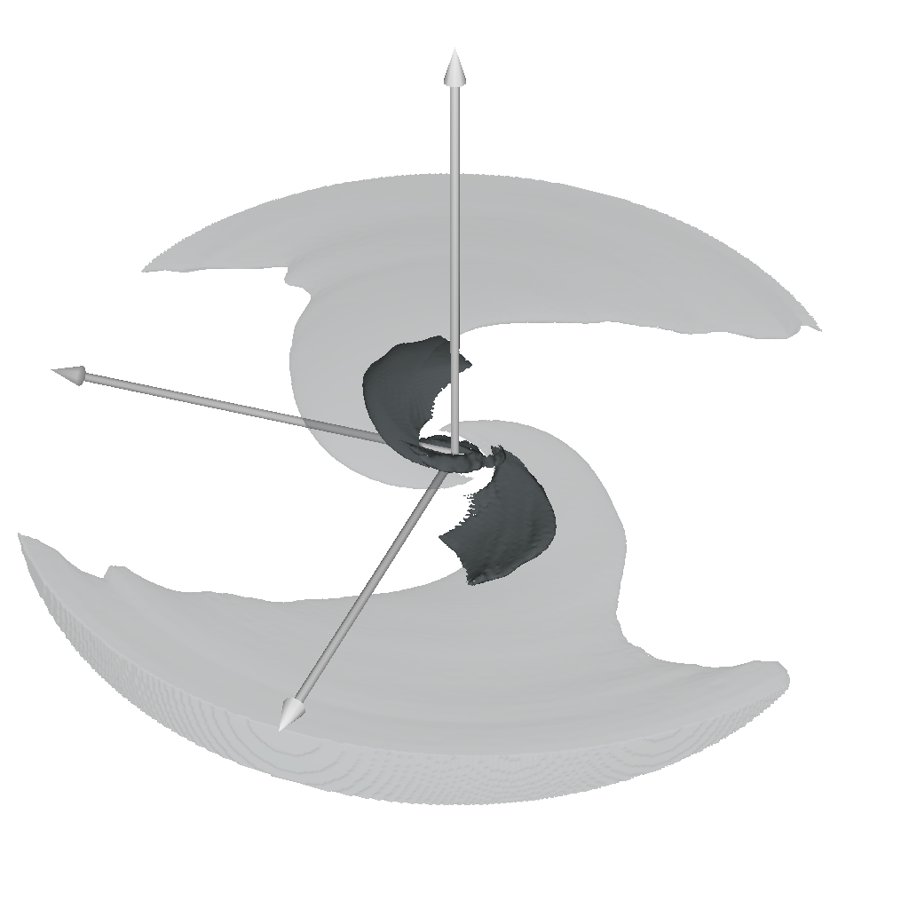
a.	b.
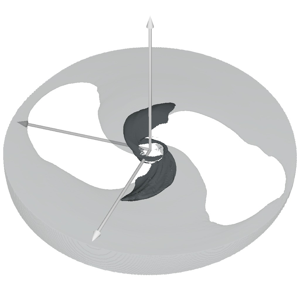
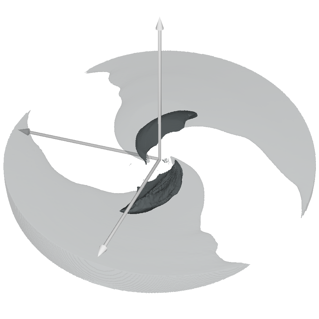
c.	d.

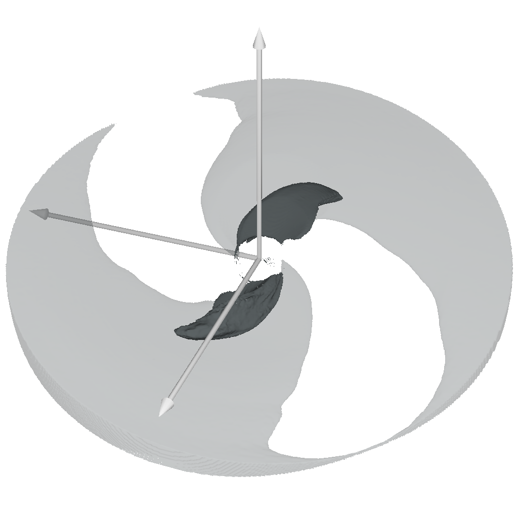
Figure 1: Three-dimensional contours in time-averaged density normalized to the time and shell-averaged density $\langle\rho\rangle_{t}/\langle\rho\rangle_{t,\theta,\phi}$ (semi-transparent gray) and Lagrangian specific entropy generation rate $\Delta s/\Delta t$ in arbitrary units [solid gray; see Equation 1] drawn at $2.5$ and $0.07$, respectively, from 910h (a), 915h (b), 915h-64a (c), and 915h-64b (d). Axes extend to $15{R_{\rm G}}$. The regions enclosed in the entropy generation rate contour identify the location of standing shock surfaces within the flow.

Table 2: Specific entropy generation rate $\Delta s/\Delta t$ per coordinate volume

Dataset	Outsidea	Insidea
910h	0.0011	0.123
915h	0.0027	0.132
915h-64a	0.0024	0.138
915h-64b	0.0017	0.154

• The average generation rate per coordinate volume inside and outside of the contours $\Delta s/\Delta t=0.07$ in Figure 1 and with $r<15{R_{\rm G}}$.

We characterize the extent and strengths of the shocks by studying the shell and time-averaged Lagrangian specific entropy generation rates, shown in Figure 2. For completeness, this figure also includes a panel for the untilted simulation which exhibits generation rates at least $50$ times smaller than those in the tilted simulations; this is consistent with the absence of standing shocks in that dataset. Each tilted simulation can be characterized by a transition from an almost constant plateau at smaller radii to the almost constant baseline at larger radii. This transition occurs more sharply in the less tilted 910h dataset. Additionally, the center of that transition region occurs at a smaller radius, around $7{R_{\rm G}}$, than in 915h and both epochs of 915h-64 where it takes place at around $10{R_{\rm G}}$. As a result, the total time and volume integrated specific entropy generation rate inside the transition region is smallest in 910h and largest in 915h-64b. Since orbital time scales away from the hole are not necessarily small compared to the simulations’ durations, one can see subtle differences at large radii in the entropy generation rate between 915h-64a and 915h-54b (panels d and e, respectively) which indicate continuing disk evolution.

a.
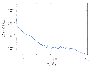
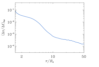
b.	c.
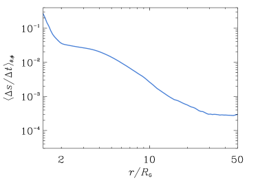
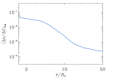
d.	e.

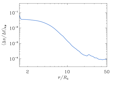
Figure 2: Time and shell-averaged specific entropy generation rate as a function of radius in 90h (a), 910h (b), 915h (c), 915h-64a (d), and 915h-64b (e).

In the $15^{\circ}$ tilted simulations, we measure compression ratios across these shock surfaces as high as $4.7$, depending on location. This is comparable to what we would expect: for a constant $5/3$ adiabatic index, as our simulations assume, hydrodynamic shocks should have a compression ratio of at most $4$, neglecting magnetic fields and relativity. We find compression ratios as high as $4.0$ in the $10^{\circ}$ simulation (Generozov et al. 2012).

Fragile & Blaes (2008) also presented comparative plots of characteristic velocities in 90h and 915h. Figure 3 reproduces these plots, only now the time-averages cover the interval $t=4$ to $10{P_{\rm orb}}$ instead of the smaller interval $t=7$ to $10{P_{\rm orb}}$, and we have also added curves for the non-radial component of the velocity and the test particle orbital velocity. Fragile & Blaes (2008) stated that the sharp upturn in $v^{r}$ indicated the start of the plunging region, and pointed out that this occurred at larger radii in the tilted simulation. Note, however, that fluid elements outside of roughly $4{R_{\rm G}}$ in the 915h tilted simulation make many complete orbits before truly plunging toward the hole. The high density arms shown in Figure 1 are therefore mostly due to postshock compression, and are not literally plunging streams, at least outside roughly $4{R_{\rm G}}$. As we discuss below, we posit that this shock compression is at the heart of the enhanced variability from spiral waves associated with transient orbiting clumps.

a.

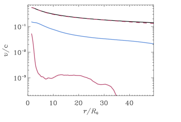
b.

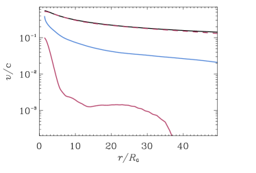
Figure 3: The time and shell-averaged radial (solid red) and non-radial (dashed red; $r\sqrt{(v^{\theta})^{2}+(v^{\phi}\sin\theta)^{2}}$) velocities, the time and shell-averaged sound speed (blue), and the test particle Keplerian orbital velocity (black) for simulations 90h (a) and 915h (b). Note that the non-radial component of the velocity very closely tracks the orbital velocity (dashed red and black, respectively) as expected. Time-averages span the interval $t=4$ to $10{P_{\rm orb}}$ and shell averages include a weighting by the time-averaged density. In both simulations, we avoid characterizing the region between $4$ and $10{R_{\rm G}}$ as “plunging” since fluid elements therein orbit the hole many times before making their final plunge toward the horizon.

4 Power Density Spectra

Our first step in probing the three-dimensional structure of variability in our simulated accretion flows is to understand the radial distribution of spectral power. Interesting structures that rotate, oscillate, or otherwise vary at characteristic frequencies may be identified in frequency space as radially extended regions with enhanced power. To this end, we follow the method outlined in our previous work (Henisey et al. 2009) and compute the shell-averaged spectral power in fluid density fluctuations,

$$P_{\rho}(f,r) \equiv\langle|\tilde{\rho}|^{2}\rangle_{\theta,\phi}/\langle\rho^{2}\rangle_{t,\theta,\phi},$$ (2)

where $\tilde{\rho}$ is the temporal Fourier transform of the (prewhitened, windowed, and padded) fluid density and is a function of space and frequency. We plot the resulting spectra for each of the five datasets in Figure 4.

a.
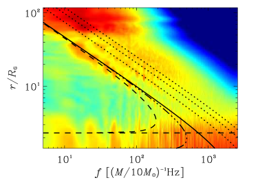
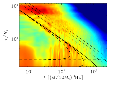
b.	c.
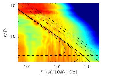
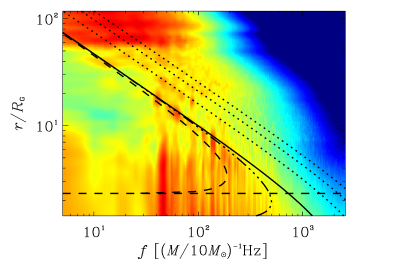
d.	e.

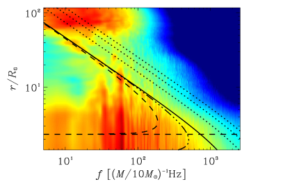
Figure 4: Shell-averaged power spectra of density $fP_{\rho}$ as a function of frequency $f$ and coordinate radius $r$ (cf. Equation 2) for datasets 90h (a), 910h (b), 915h (c), 915h-64a (d), and 915h-64b (e). Over-plots include the orbital frequency (solid) and its harmonics (dotted), the geodesic radial epicyclic frequency and the ISCO radius (dashed), and the geodesic vertical epicyclic frequency (triple-dot dashed).

Two features in these spectra warrant discussion. First, in Henisey et al. (2009) we showed that transient clumps traveling on roughly Keplerian trajectories exist amid the MRI turbulence in simulations 90h and 915h. They appear as enhanced power along the curve of orbital frequency versus radius. In Figure 4, we now clearly see that these orbiting clumps arise generically in all five of our datasets.

Second, a set of features that we previously identified in 915h in Henisey et al. (2009) likewise appear here strongly in each of the tilted simulations. Specifically, the tilted datasets exhibit significant power in vertical streaks extending inward in radius from the orbital frequency curve. For the remainder of this work, we will refer to such power as “intraorbital”, denoting that it is power at a specific frequency and at all radii inward of the frequency’s corotation radius. Importantly, these intraorbital, coherent structures coincide with the power enhancements along the orbital frequency curve associated with orbiting clumps. In the next section, we explore the relationship between these intraorbital features and their respective orbital clumps.

In Henisey et al. (2009), we concentrated much of our study on the $118{\rm Hz}$ feature in the 915h simulation. Here we note that strong vertical tracks also appear in 910h at $150{\rm Hz}$, in 915h-64a at $140{\rm Hz}$, and in 915h-64b at $60{\rm Hz}$. Noting that 915h-64a and 915h-64b represent different epochs of the same simulation and that 915h and 915h-64a differ only in there initial random perturbations, variety in the position of and power in these simulations’ vertical streaks indicates that while these structures are long lived with respect to the local orbital period, they are nonetheless transient features: they come and go on time scales smaller than but comparable to the simulation durations. While these intraorbital streaks appear exclusively in the tilted simulations, features that are similar in structure though markedly weaker (by perhaps as large a factor as 30) in spectral power exist within the untilted flow. One such example appears at $110{\rm Hz}$. Note that in all cases (both tilted and untilted), a local minimum seems to occur along the vertical track at roughly the midpoint between the corotation radius and innermost stable circular orbit (ISCO).

These intraorbital power features contribute to generally enhanced variability in each of the tilted simulations at all frequencies greater than approximately $50{\rm Hz}$ (equivalently, the orbital frequency at roughly $15{R_{\rm G}}$) and radially inward of the orbital frequency curve. There appears to be a qualitative trend of increasing intraorbital power with increasing tilt and with more advanced flow evolution, though we have not attempted to quantitatively assess its significance.

To summarize, Figure 4 confirms that transient over-dense clumps orbiting with the background flow are generic in our simulations. The mechanism responsible for the formation of these clumps remains unexplained. In terms of our global variability study however, it is sufficient that these clumps exist and that, above some frequency threshold, they are associated with radially extended power at the same frequency as the clump’s orbital frequency. This intraorbital spectral power is significantly enhanced in the tilted datasets compared to that observed in the untilted simulation. Beyond identifying these variability features, however, there is little more to glean from this shell-averaged analysis. The next section, therefore, studies the full three-dimensional behavior of these structures at specific frequencies and aims to understand the variability in the context of the background structure discussed in Section 3.

5 Structural Analysis

We now study the variability discussed in the previous section by analyzing its spatial structure and temporal behavior in more detail. In Section 5.1, we visualize the orbiting clumps and their associated intraorbital variability within the context of the flow’s nonaxisymmetric background and analyze the temporal phase relationships across the spatial extent of the high-power variability. In Section 5.2, we then put forward a unified physical model that explains those spectral features in each dataset.

5.1 Spatial structure of variability

The coherent structures identified in Section 4 represent density perturbations throughout the disk varying at specific frequencies. We can therefore visualize these structures by filtering away any fluctuations that occur on greater or smaller time scales. Mathematically, we construct a frequency-filtered density,

$$\rho_{\omega}(t,\vec{r})=R_{\omega}\cos{\omega t}+I_{\omega}\sin{\omega t},$$ (3)

where $R_{\omega}\equiv 2{\rm Re}[\tilde{\rho}(\omega,\vec{r})]$ and $I_{\omega}\equiv 2{\rm Im}[\tilde{\rho}(\omega,\vec{r})]$ are twice the real and imaginary parts of the Fourier transform of the density time-series. The factor of $2$ accounts for the fact that Fourier transforms of real-valued functions like our density are even in frequency space, splitting total power evenly between positive and negative frequencies. With the above definitions then, we can restrict our study to positive frequencies. This density represents only those perturbations of the flow that vary with angular frequency $\omega$, and therefore, although the time $t$ directly relates to the simulation coordinate time, we only need to study the function’s evolution through a single period $0\leq t<2\pi/\omega$. Figure 5 shows snapshots in time of contours of frequency-filtered density normalized in a manner consistent with the spectra in Figure 4, that is, $\rho_{\omega}\sqrt{\omega/2\pi\langle\rho^{2}\rangle_{t,\theta,\phi}}$. For each dataset, we have evaluated the filtered density at frequencies that exhibit significant intraorbital power in Figure 4. We have selected moments within the oscillation period that most clearly illustrate that this intraorbital power is spatially concentrated near the background’s over-dense arms. The contours lie at $0.125$ for datasets 910h, 915h, and 915h-64a and $0.175$ for dataset 915h-64b.

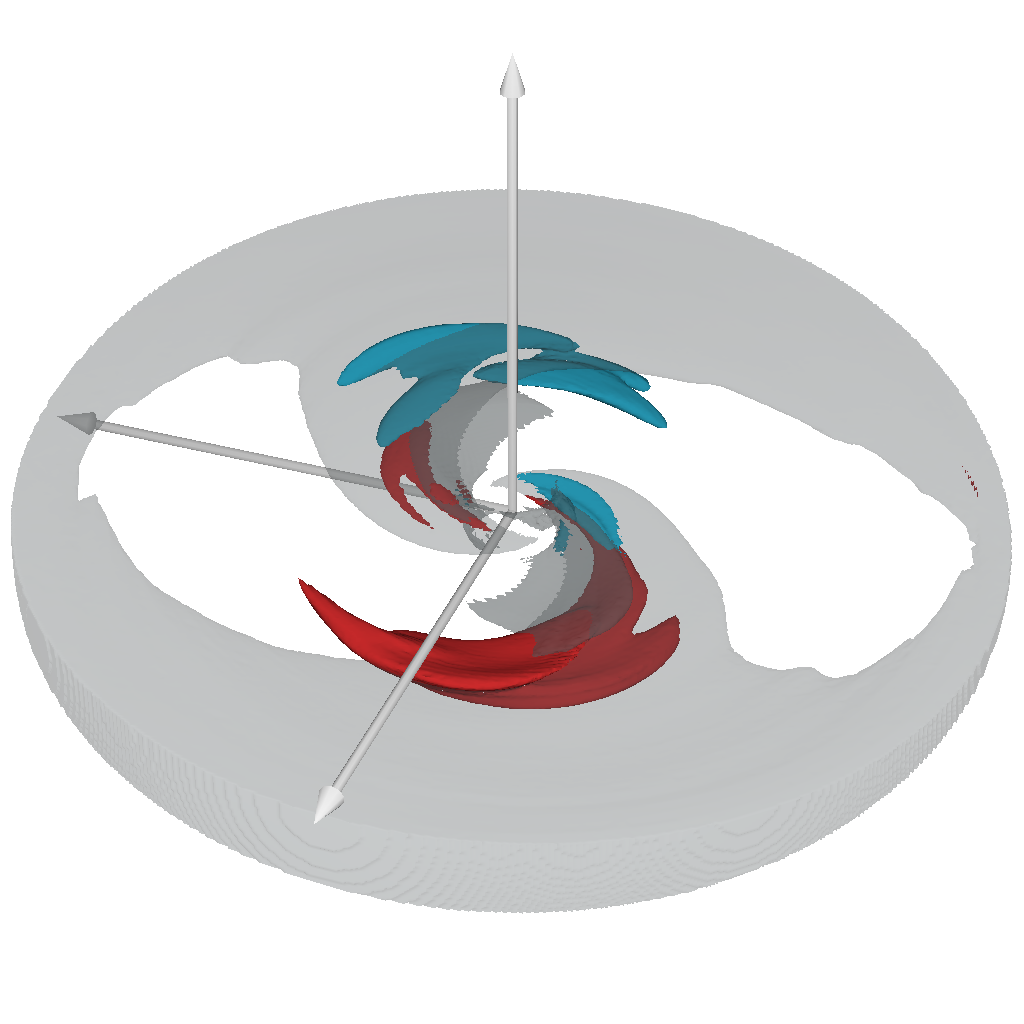
a.	b.
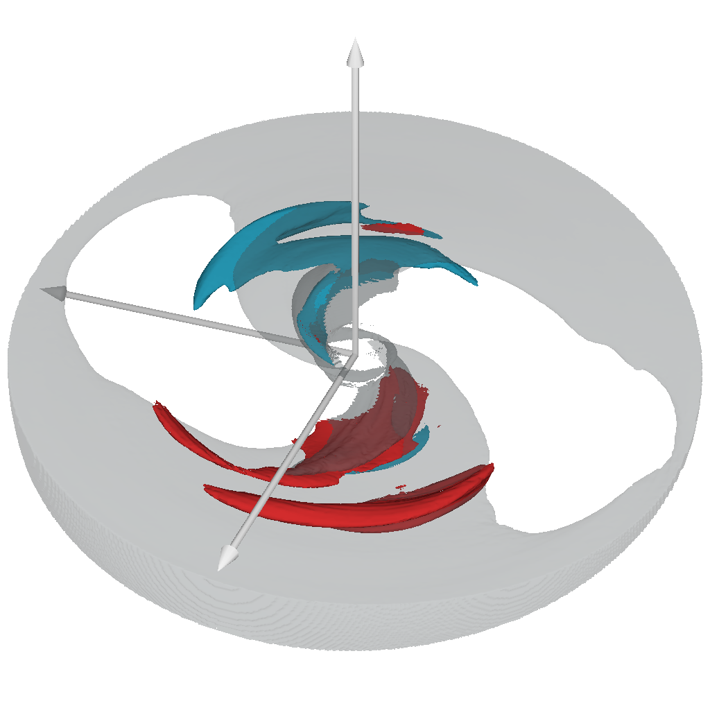
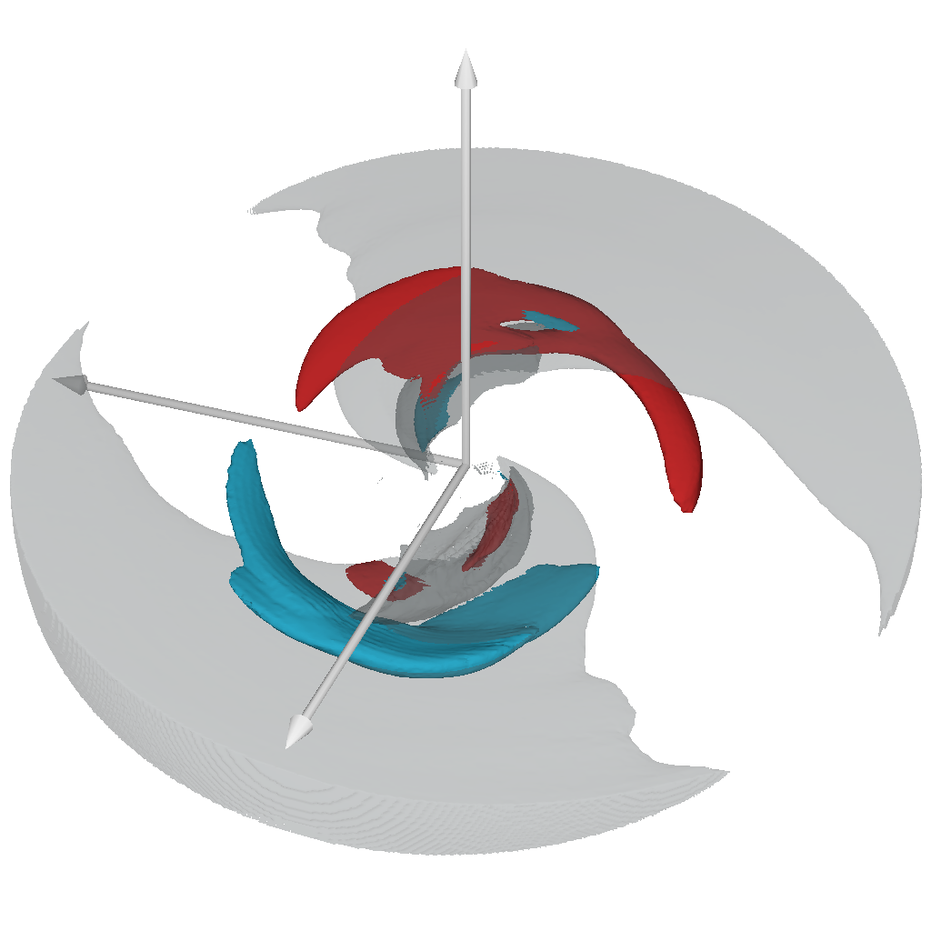
c.	d.

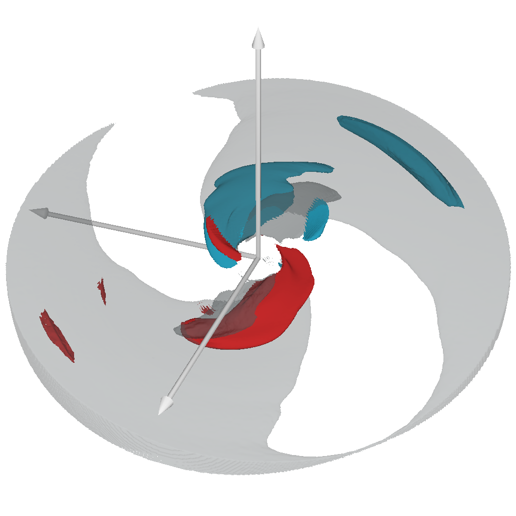
Figure 5: Three-dimensional visualizations of the spatial structure of the variability in density for oscillations at $150{\rm Hz}$ in 910h (a), at $118{\rm Hz}$ in 915h (b), at $140{\rm Hz}$ in 915h-64a (c), and at $60{\rm Hz}$ in 915h-64b (d). Specifically, we depict contours of the frequency-filtered density (see Equation 3) normalized in a manner consistent with the spectra in Figure 4, that is, $\rho_{\omega}\sqrt{\omega/2\pi\langle\rho^{2}\rangle_{t,\theta,\phi}}$. These surfaces lie at positive (red) and negative (blue) $0.125$ in 910h, 915h, and 915h-64a and $0.175$ in 915h-64b. For reference, semitransparent surfaces indicate density (light gray) and specific entropy generation rate (dark gray) contours identical to those in Figure 1. Axes extend to $15{R_{\rm G}}$.

Variability at the given frequencies in each tilted dataset spatially manifests itself in two forms: a clump orbiting near the corotation radius and peaking in amplitude after passing the shock fronts, and a pulsation within each over-dense arm just past the shocks and inside the corotation radius. The latter feature is responsible for the previously identified intraorbital power.

Four explanations for this variability structure seem plausible. First, after interacting with the shock, the orbiting clump may, by some mechanism, liberate some small amount of material which would fall along the arms toward the hole. Second, after interacting with the shock, the orbiting clump may send a pressure wave down the over-dense arm. Third, standing inertial waves may be trapped within the over-dense arms and be excited and maintained by the clump-shock interaction. Fourth, a coherent acoustic spiral pattern produced and maintained by an orbiting clump may interact with the radially extended shock, increasing the amplitude of both the clump and spiral independently.

In light of our conclusions in Section 3, we rule out the first explanation since sloughed off material cannot simply fall past the otherwise roughly Keplerian flow circulating around the hole. Similarly, a close examination of the temporal phase relationships within the pulses forces us to discard the second and third explanations. Specifically, Figure 6 shows six successive snapshots in time of the $118{\rm Hz}$ variability, that is, of the frequency-filtered density given by Equation 3. The time interval between each frame is $1/40$th of the oscillation’s period. By construction, these structures vary at the filter frequency, in this case, $118{\rm Hz}$, regardless of any local characteristic frequencies like the orbital frequency. Notice that the red variability structure inside the over-dense arm closest to the viewer (arrow $3$) appears to start at small radius and moves outward toward larger radii. Likewise, two additional structures (labeled $2$ and $4$) appear to recede away from the center. Since the second and third hypotheses predict an inwardly propagating wave and a standing wave within the arms, respectively, this behavior rules out both models.

Figure 6: Successive three-dimensional snapshots in time of the $118{\rm Hz}$ pattern in the 915h simulation given by normalized frequency-filtered density (see Figure 5). By construction, this variability is independent of any local characteristic frequencies like the orbital frequency. Each frame is separated by $1/40$th of a full oscillation period. Semi-transparent surfaces (light and dark gray) and positive (red) and negative (blue) contours lie at the same levels as in Figure 5. Numbered arrows track the location of the trailing ($1$) and leading ($5$) edges of the orbiting clump as well as three edges of the flashes in the over-dense arms: one which advances outwardly from the hole ($3$) and two that recede away from it ($2$ and $4$). Axes extend to $15{R_{\rm G}}$.

In the fourth hypothesis however, a radially extended spiral pattern rotates bodily about the hole at the same frequency (here $118{\rm Hz}$) as its associated corotating clump. Depending on the shape of the spiral relative to a shock surface, the point of interaction between the two may appear to move inward or outward in time along the shock’s face. For example, if some segment of the spiral is trailing, the interaction point between it and the stationary shock surface will appear to move outward in time, akin to structure $3$ in Figure 6. In this way, a spiral-shock interaction model permits all the complex temporal relationships depicted in Figure 6. Of our four hypotheses, this remains the only plausible explanation.

At the spiral-shock interaction point, the acoustic wave passing through the shock will experience an enhancement in its density amplitude (as defined by half the difference between the maximum and minimum density in the wave) equal to the shock compression ratio discussed in Section 3. In the $15^{\circ}$ tilted simulations, the ratios were as high as $4.7$ while in the $10^{\circ}$ tilted simulation they were as large as $4.0$ (Generozov et al. 2012). We therefore expect density power in the acoustic waves (which goes as the square of the amplitude) to be enhanced by a factor of roughly $22$ in the $15^{\circ}$ tilted simulation, and $16$ in the $10^{\circ}$ tilted simulations, as compared to the untilted simulation. This quantitatively matches the larger intraorbital power in the vertical streaks in the tilted simulations as compared to the untilted simulation in the density power spectra shown in Figure 4. This spiral-shock interaction model can explain both the apparent motion of the variability along the background over-dense arms and the magnitude of the increased variability at the point of interaction.

5.2 Prograde and retrograde decomposition

Of those models described above that aim to explain the apparent movement of perturbations along the over-dense arms, only that in which a rotating acoustic spiral accompanies the orbiting clumps identified in Section 4 and visualized in section 5.1 is consistent with the observed temporal relationships. In an axisymmetric background akin to that in our untilted simulation, for example, such a spiral pattern should be both stationary in a frame corotating with the clump and largely $m=1$ in its azimuthal symmetry. By assuming these characteristics, this section further decomposes the variability in our simulations to locate these spiral structures and better understand their physical nature.

Since the structures visualized in the previous section are largely $m=1$, we first isolate this component of the variability from the frequency-filtered time series in Equation 3. In other words, we project the spatial functions $R_{\omega}$ and $I_{\omega}$ onto the two $m=1$ spatial basis functions so that

$$\rho_{\omega,m=1} =(R_{\omega,{\rm c}}\cos{\phi}+R_{\omega,{\rm s}}\sin{\phi})\cos{\omega t}$$

$$\qquad+(I_{\omega,{\rm c}}\cos{\phi}+I_{\omega,{\rm s}}\sin{\phi})\sin{\omega t},$$ (4)

where

$$R_{\omega,{\rm c}} =\frac{1}{\pi}\int_{0}^{2\pi}R_{\omega}\cos{\phi}\,d\phi$$ (5a)

$$R_{\omega,{\rm s}} =\frac{1}{\pi}\int_{0}^{2\pi}R_{\omega}\sin{\phi}\,d\phi$$ (5b)

$$I_{\omega,{\rm c}} =\frac{1}{\pi}\int_{0}^{2\pi}I_{\omega}\cos{\phi}\,d\phi$$ (5c)

$$I_{\omega,{\rm s}} =\frac{1}{\pi}\int_{0}^{2\pi}I_{\omega}\sin{\phi}\,d\phi.$$ (5d)

Using basic trigonometric identities, one can combine these terms in a straight-forward manner to find

$$\rho_{\omega,m=1} =A_{\omega}\cos(\phi-\omega t-\alpha_{\omega})$$

$$\qquad+B_{\omega}\cos(-\phi-\omega t-\beta_{\omega}),$$ (6)

where

$$A_{\omega}^{2} =\frac{1}{4}\left[\left(R_{\omega,{\rm c}}+I_{\omega,{\rm s}}\right)^{2}\right.$$

$$\qquad\left.+\left(R_{\omega,{\rm s}}-I_{\omega,{\rm c}}\right)^{2}\right]$$ (7a)

$$B_{\omega}^{2} =\frac{1}{4}\left[\left(R_{\omega,{\rm c}}-I_{\omega,{\rm s}}\right)^{2}\right.$$

$$\qquad\left.+\left(R_{\omega,{\rm s}}+I_{\omega,{\rm c}}\right)^{2}\right]$$ (7b)

$$\tan\alpha_{\omega} =\frac{R_{\omega,{\rm s}}-I_{\omega,{\rm c}}}{R_{\omega,{\rm c}}+I_{\omega,{\rm s}}}$$ (7c)

$$\tan\beta_{\omega} =\frac{-R_{\omega,{\rm s}}-I_{\omega,{\rm c}}}{R_{\omega,{\rm c}}-I_{\omega,{\rm s}}}.$$ (7d)

Given the form of the arguments within each cosine, we can now interpret the coefficients $A_{\omega}$ and $B_{\omega}$ as the amplitudes of the two rotating components, a prograde pattern and a retrograde pattern, respectively, at each $(r,\theta)$ pair.

Four basic motions can result from this interpretation on a given ring of constant $r$ and $\theta$. Clearly, if $A_{\omega}$ or $B_{\omega}$ is zero, one would observe a purely retrograde or prograde motion, respectively. Similarly, $A_{\omega}=B_{\omega}$ indicates a standing wave structure. Less intuitively, the more general case in which $0<B_{\omega}<A_{\omega}$ turns out to be a prograde pattern that no longer exhibits a constant amplitude or rotation speed. Like two sinusoidal waves of differing amplitudes crossing on a string, the two components constructively interfere at some moments producing a large density perturbation (of magnitude $|A_{\omega}|+|B_{\omega}|$) that rotates in a prograde manner at an instantaneous angular speed smaller than the angular frequency of the oscillation. In the same way, at the moments when the two components destructively interfere, they produce a lower amplitude perturbation (having magnitude $|A_{\omega}|-|B_{\omega}|$) that again rotates in a prograde fashion but now with an instantaneous angular speed greater than the angular frequency of the oscillation.

Keeping these possible motions in mind, we return to our untilted and tilted disks. In the axisymmetric background of the untilted simulation, the decomposition of a clump with a corotating spiral ought to return a purely prograde pattern. On the other hand, we suggested in Section 5.1 that the standing shocks associated with the non-axisymmetric background amplify the density of the clump and its corotating spiral in the tilted simulations. We therefore expect to find a predominantly prograde spiral throughout the region interior to the clump accompanied by a weaker but nonzero retrograde component. This latter piece merely accounts for the fact that the complete perturbation has a higher magnitude and slower rotation speed just past the standing shocks and a lower amplitude and faster rotation speed away from the shocks. This result aligns well with the structure and evolution depicted in Figures 5 and 6, respectively.

We plot in Figure 7 the power in each rotating component, $\langle|A_{\omega}|^{2}\rangle_{\theta}$ and $\langle|B_{\omega}|^{2}\rangle_{\theta}$ at the indicated frequencies and as a function of radius, normalizing to match Figure 4. As anticipated, the $m=1$ variability in the untilted simulation is dominated by a prograde pattern at all radii and shows very little power in the retrograde term. We take this as evidence that the weak intraorbital variability found in the power spectra in Figure 4 for the untilted simulation arises from prograde spirals corotating with Keplerian clumps.

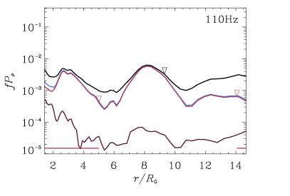
a.	b.
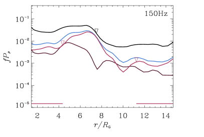
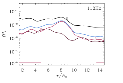
c.	d.
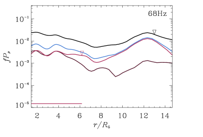
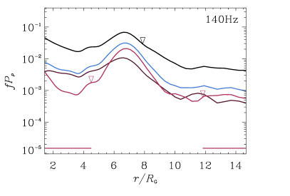
e.	f.

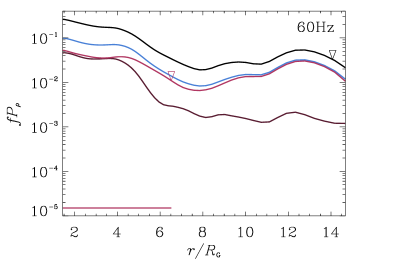
Figure 7: Total power at specified frequencies (black; $\langle R_{\omega}^{2}+I_{\omega}^{2}\rangle_{\theta,\phi}$) in 90h (a), 910h (b), 915h (c and d), 915h-64a (e), and 915h-64b (f) compared with the power in the $m=1$ projection at the indicated frequencies (blue; $\langle A_{\omega}^{2}+B_{\omega}^{2}\rangle_{\theta}$). The projected power is further decomposed into its prograde (light red; $\langle A_{\omega}^{2}\rangle_{\theta}$) and retrograde (dark red; $\langle B_{\omega}^{2}\rangle_{\theta}$) contributions. Note that all curves have been multiplied by $\omega/2\pi\langle\rho^{2}\rangle_{t,\theta,\phi}$ to match the normalization of the spectra in Figure 4. Triangles mark the test particle corotation radius (black) and $m=1$ Lindblad resonances (light red). Light red, horizontal lines mark propagation regions for $n=0$, $m=1$ modes.

For the tilted simulations, Figure 7 shows that the clump is likewise dominated by prograde motion. We interpret the prograde pattern as, in some sense, the average power profile of the clump’s associated spiral. Additionally though, we also see an enhanced retrograde component and interpret the relative retrograde to prograde power as the degree to which the shock amplifying background deforms the spiral as it rotates around the disk. We emphasize that one must only interpret the retrograde power as a mathematical tool; it cannot be any kind of physical structure. If it were a real, propagating perturbation, it would be traveling upstream, against the background fluid flow at speeds which far exceed the local sound speed. Nonetheless, the largely prograde nature of the variability corroborates the clump-spiral hypothesis in both untilted and tilted configurations and further indicates that the standing shocks associated with tilted geometries enhance variability by effectively amplifying passing density fluctuations.

Shock amplification and tilt aside, we characterize the nature of these apparently ubiquitous, prograde spiral patterns by comparing the structure of their prograde components to diskoseismic predictions. Isothermal diskoseismic models of untilted, flat disks indicate that short wavelength WKB perturbations with local radial wave number $k$ obey the dispersion relation (Okazaki et al. 1987),

$$k^{2}=\frac{(\hat{\omega}^{2}-\kappa_{r}^{2})(\hat{\omega}^{2}-n\kappa_{\theta}^{2})}{\hat{\omega}^{2}c_{\rm s}^{2}},$$ (8)

where $\hat{\omega}\equiv\omega-m\Omega$ is the Doppler-shifted wave frequency, $\kappa_{r}$ is the radial epicyclic frequency, and $n$ is a non-negative integer that indicates the number of vertical nodes in the oscillation. Adopting the hypothesis that our prograde spiral patterns represent $n=0$, $m=1$ acoustic perturbations having angular frequency $\omega$, then the region around the corotation radius bounded by the inner and outer Lindblad resonances is an evanescent region with local radial decay constant $a_{\rm disp}$ such that $k=ia_{\rm disp}$. If the WKB approximation holds, we can directly calculate the local radial decay rate of the amplitude of the prograde spiral using a derivative of the power in Figure 7, specifically,

$$a=\frac{1}{2}\frac{d}{dr}\left\{\log{\left[\frac{\omega}{2\pi}\frac{\langle A_{\omega}^{2}\rangle_{\theta}}{\langle\rho^{2}\rangle_{t,\theta,\phi}}\right]}\right\}.$$ (9)

If our spirals are acoustic in nature, then up to its sign, this calculated radial decay rate should roughly match the theoretical decay constant $a_{\rm disp}$, that is, the imaginary component of the wave number from Equation 8. In Figure 8, we plot both $a$ and $a_{\rm disp}$. While there is noise, it is noteworthy that the measured decay rate in each simulation is positive inside corotation, negative outside corotation, and approximately equal in magnitude to that predicted by the dispersion relation in Equation 8. We believe that this further supports the hypothesis that intraorbital power is the manifestation of spirals excited by orbiting clumps that are acoustic in nature.

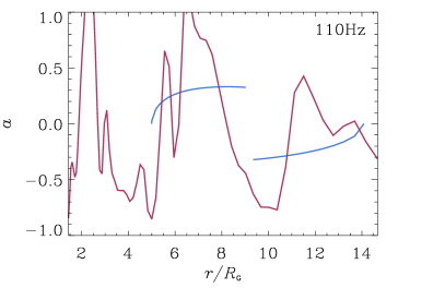
a.	b.
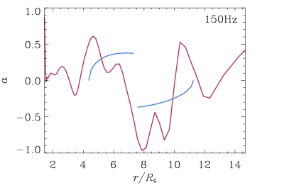
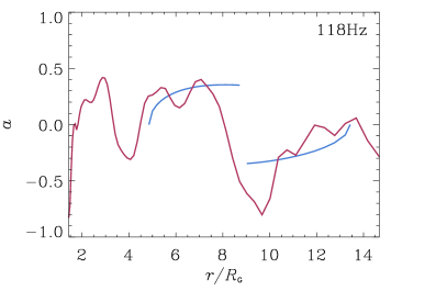
c.	d.
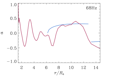
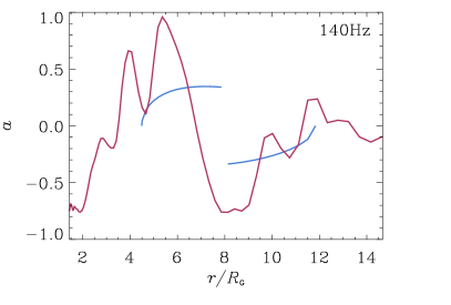
e.	f.

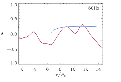
Figure 8: Local radial decay rate $a$ (red; see Equation 9) in the prograde, $m=1$ component of variability compared with the local radial decay constant $a_{\rm disp}$ (blue; positive inside corotation, negative outside corotation) predicted from the dispersion relation in Equation 8 at specified frequencies in 90h (a), 910h (b), 915h (c and d), 915h-64a (e), and 915h-64b (f).

To aid in the visualization of these spiral patterns, Figure 9 depicts a snapshot in time of the location (in an average sense) of the maxima of the prograde pattern at each radius, that is, $\overline{\alpha_{\omega}}\equiv\arctan{\left[\langle R_{\omega,{\rm s}}-I_{\omega,{\rm c}}\rangle_{\theta}/\langle R_{\omega,{\rm c}}+I_{\omega,{\rm s}}\rangle_{\theta}\right]}$ inspired by the definition of $\alpha_{\omega}$ in Equation 7. We interpret the shape of these curves as the average shape of the clump-spiral structure. One can imagine that these plots evolve in time by noting that the prograde spiral will rotate counterclockwise through the stationary background flow. Breaking down their structure, we see that the prograde spirals from each simulation share the same, qualitative, three-segment geometry: a trailing segment at small radii, a leading segment around an intermediate radius near the inner Lindblad resonance, and another trailing segment terminating at the corotating clump.

The first and last segments of these spirals seem consistent with the outward moving density fluctuations located in the over-dense arm and identified in Figure 6 by labels $2$, $3$, and $4$. Since $2$ and $3$ appear over roughly the same range of radii in their respective arms, our $m=1$ spiral model would predict that the two perturbations should be spatially symmetric though half a period out of phase in time. Looking closely however, we see that while $2$ is retreating away from the hole and $3$ is growing toward larger radii, they are both nonetheless simultaneously positive. This indicates that feature $2$ leads $3$ in phase by slightly less than half a period. This behavior must be due to $m>1$ contributions to the overall clump/spiral structure, though we have not analyzed these higher order effects in detail.

Given the above, one might anticipate that the middle, leading segment ought to have an associated inward moving density enhancement in each over-dense arm. The absence of such features in Figure 6 has a two-fold explanation. First, Figure 9 only roughly depicts the location of the spiral’s maximum at each radius and not the maxima’s relative amplitudes. As seen in Figure 7, the density perturbations ubiquitously reach local minima near the Lindblad resonances and, correspondingly, the leading segments of the spirals must be relatively weak. These perturbations therefore have little effect in Figure 6. Second, the retrograde component (not shown in Figure 9 for purposes of clarity) is oriented such that the whole leading segment reaches its maxima all at once and without any apparent motion. Although we strongly suspect that there is some connection between the common shape of these spirals and the location of the inner Lindblad resonances, it is unclear what mechanism might be responsible for the apparent correlations.

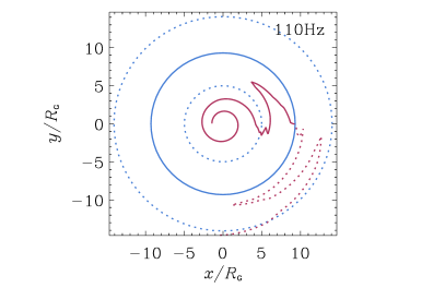
a.	b.
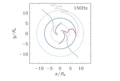
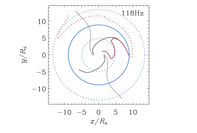
c.	d.
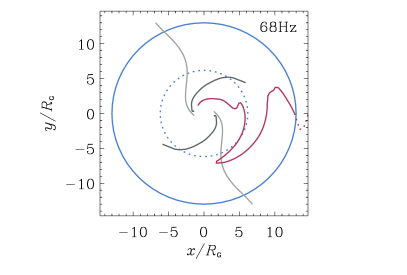
e.	f.

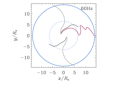
Figure 9: Snapshots of the spatial position of the maxima of the prograde pattern of the $m=1$ mode power at each radius (red; solid inward and dotted outward of corotation) for patterns at the indicated frequencies in 90h (a), 910h (b), 915h (c and d), 915h-64a (e), and 915h-64b (f). For reference, we plot the approximate location of the background density maxima (light gray) and shock surfaces (dark gray) as well as circles marking the test-particle corotation radius (solid blue) and inner and outer Lindblad resonances (dashed blue). The prograde pattern rotates counterclockwise in time with respect to the density maxima and shock surfaces.

To summarize, orbiting clumps and their accompanying spiral patterns are generic in these simulations. Although these features do little to increase the overall variability in untilted disk geometries, the standing shocks characteristic of tilted simulations interact strongly with the orbiting spirals, producing regions of higher density where the two come into contact. Since the trailing segments of spiral pattern are more tightly wound than the standing shocks, the high density region appears to move outwardly along the shock surfaces. This mechanism explains the complex behavior shown in Figure 6 and provides an explanation for the characteristically higher variability at suborbital frequencies seen exclusively in tilted geometries.

6 Conclusions

In our previous paper (Henisey et al. 2009), we identified variability at frequencies comparable to those expected for inertial modes (i.e. below the local radial epicyclic frequency) in the inner parts of a GRMHD simulation of a tilted accretion flow (915h). This appeared to provide preliminary confirmation that warps and eccentricity might excite inertial modes even in the presence of MRI turbulence in accretion disks (Kato 2004a, 2009; Ferreira & Ogilvie 2008), whereas in shearing box and global untilted flow simulations, such inertial modes are destroyed by MRI turbulence (Arras et al. 2006; Reynolds & Miller 2009). However, our more complete analysis here of simulation 915h, along with other tilted simulations 910h and 915h-64, shows that the three-dimensional structure of the enhanced variability at suborbital frequencies is not consistent with the excitation of trapped inertial modes.

The variability that we observe is in fact present in both untilted and tilted simulations, and originates from transient over-dense clumps of material co-orbiting with the background flow and randomly located at nearly all radii. Exhibiting a predominantly $m=1$ azimuthal structure, such fluctuations are likely only to manifest themselves in simulations which incorporate a complete $2\pi$ treatment of the azimuthal angle. We note that Dolence et al. (2012) also identified $m=1$ structures in their global GRMHD simulations that appeared to be associated with the QPO they identified in their radiative post-processing of these simulations. It may be that these structures are similar to the clumps that we have identified in our work. In any case, the formation mechanism for these clumps remains unclear. Given that they orbit with the background flow, it may be that they are generated by some instability associated with a corotation resonance (e.g. Fu & Lai 2011), but this requires further study.

We find that these orbiting clump structures are accompanied by extended acoustic spiral waves with pattern speeds equal to the orbital angular velocity of the clump. Exhibiting power which exponentially decreases away in radius from the orbit of the clump, these spirals are consistent with forced acoustic perturbations inside the otherwise evanescent region surrounding the corotation resonance (Okazaki et al. 1987). In the untilted simulation 90h, these spiral perturbations are quite weak. As shown by Fragile & Blaes (2008), however, converging eccentric orbits in tilted accretion flows produce two standing shock surfaces which precede two over-dense arms. The compression of the orbiting flow at these shocks amplifies the density amplitude of the otherwise weak acoustic spirals, thereby greatly enhancing their variability power signature. We therefore hypothesize that, given a greater tilt, any moderately thick accretion flow will exhibit greater variability at frequencies comparable to the orbital frequencies at all radii inward of perhaps $10$ to $15{R_{\rm G}}$, that is, the furthest radial extent of the shocks.

These findings are quite relevant to a recent class of models which produce a low-frequency QPO in a hot, somewhat tilted, inner flow that is qualitatively consistent with observations of black hole X-ray binaries (Ingram et al. 2009; Ingram & Done 2011). Such tilted flows naturally precess at a Lense-Thirring precession frequency determined by the hot flow’s outermost edge (Fragile et al. 2007). Therefore, in these low-frequency QPO models, we predict increased continuum variability at frequencies greater than the orbital frequency measured at either the hot flow’s outer cutoff radius or the termination radius of the standing shocks, whichever is closer to the hole.

Over short intervals of time, the variability due to the clumps and spirals occurs at discrete frequencies depending on which clumps happen to be present. While these frequencies are comparable to high-frequency QPOs in black hole X-ray binaries, the transient nature of the clumps implies that they cannot produce robust high-frequency QPOs, and are likely instead to just contribute to enhanced continuum variability as we noted above. We have not identified any other potential high-frequency QPO candidates in our simulations. We appear to be in the good company of many other accretion simulations to date, and we suspect that either the QPO is too weak to detect in current numerical simulations or, more likely, that the QPO requires physics which is not yet captured by our numerical simulations. As Reynolds & Miller (2009) point out, current global simulations lack the necessary treatment of radiation physics to accurately simulate the near Eddington limited accretion which characterizes the steep power-law spectral state uniquely associated with the high-frequency QPO. Therefore, in the coming years when new numerical methods meet more advanced computational technologies, variability studies akin to those we have presented here will become increasingly relevant in understanding the complex dynamics associated with black hole accretion flows.

We thank Lars Bildsten for useful conversations, and Aleksey Generozov and Julia Wilson for help in analyzing the density compression ratios of the shocks. This work was supported in part by NSF grant AST-0707624. PCF acknowledges support from the National Science Foundation under grants AST-0807385 and PHY11-25915.

References

- Anninos et al. (2005) Anninos, P., Fragile, P. C., & Salmonson, J. D. 2005, ApJ, 635, 723
- Arras et al. (2006) Arras, P., Blaes, O., & Turner, N. J. 2006, ApJ, 645, L65
- Balbus & Hawley (1991) Balbus, S. A., & Hawley, J. F. 1991, ApJ, 376, 214
- Chakrabarti (1985) Chakrabarti, S. K. 1985, ApJ, 288, 1
- Churazov et al. (2001) Churazov, E., Gilfanov, M., & Revnivtsev, M. 2001, MNRAS, 321, 759
- Dexter & Fragile (2011) Dexter, J., & Fragile, P. C. 2011, ApJ, 730, 36
- Dolence et al. (2012) Dolence, J. C., Gammie, C. F., Shiokawa, H., & Noble, S. C. 2012, ApJ, 746, L10
- Ferreira & Ogilvie (2008) Ferreira, B. T., & Ogilvie, G. I. 2008, MNRAS, 386, 2297
- Fragile & Anninos (2005) Fragile, P. C., & Anninos, P. 2005, ApJ, 623, 347
- Fragile & Blaes (2008) Fragile, P. C., & Blaes, O. M. 2008, ApJ, 687, 757
- Fragile et al. (2007) Fragile, P. C., Blaes, O. M., Anninos, P., & Salmonson, J. D. 2007, ApJ, 668, 417
- Fu & Lai (2011) Fu, W., & Lai, D. 2011, MNRAS, 410, 399
- Generozov et al. (2012) Generozov, A., Blaes, O. M., Fragile, P. C., & Henisey, K. B. 2012, in preparation
- Henisey et al. (2009) Henisey, K. B., Blaes, O. M., Fragile, P. C., & Ferreira, B. T. 2009, ApJ, 706, 705
- Ingram & Done (2011) Ingram, A., & Done, C. 2011, MNRAS, 415, 2323
- Ingram et al. (2009) Ingram, A., Done, C., & Fragile, P. C. 2009, MNRAS, 397, L101
- Kato (2001) Kato, S. 2001, PASJ, 53, 1
- Kato (2004a) —. 2004a, PASJ, 56, 905
- Kato (2008) —. 2008, PASJ, 60, 111
- Kato (2009) —. 2009, PASJ, 61, 1237
- Kato (2004b) Kato, Y. 2004b, PASJ, 56, 931
- Machida & Matsumoto (2008) Machida, M., & Matsumoto, R. 2008, PASJ, 60, 613
- Noble & Krolik (2009) Noble, S. C., & Krolik, J. H. 2009, ApJ, 703, 964
- Okazaki et al. (1987) Okazaki, A. T., Kato, S., & Fukue, J. 1987, PASJ, 39, 457
- O’Neill et al. (2011) O’Neill, S. M., Reynolds, C. S., Miller, M. C., & Sorathia, K. A. 2011, ApJ, 736, 107
- Remillard & McClintock (2006) Remillard, R. A., & McClintock, J. E. 2006, ARA&A, 44, 49
- Reynolds & Miller (2009) Reynolds, C. S., & Miller, M. C. 2009, ApJ, 692, 869
- Schnittman et al. (2006) Schnittman, J. D., Krolik, J. H., & Hawley, J. F. 2006, ApJ, 651, 1031
- Wagoner (1999) Wagoner, R. V. 1999, Phys. Rep., 311, 259