Semileptonic $\boldmath{B}$ to $\boldmath{D}$ decays at nonzero recoil with 2+1 flavors of improved staggered quarks

Abstract:

The Fermilab Lattice and MILC collaborations are completing a comprehensive program of heavy-light physics on MILC (2+1)-flavor asqtad ensembles with lattice spacings as small as 0.045 fm and light-to-strange-quark mass ratios as low as 1/20. We use the Fermilab interpretation of the clover action for heavy valence quarks and the asqtad action for the light valence quarks. The central goal of the program is to provide ever more exacting tests of the unitarity of the CKM matrix. We present preliminary results for one part of the program, namely the analysis of the semileptonic decay $B\rightarrow D\ell\nu$ at nonzero recoil.

1 Introduction

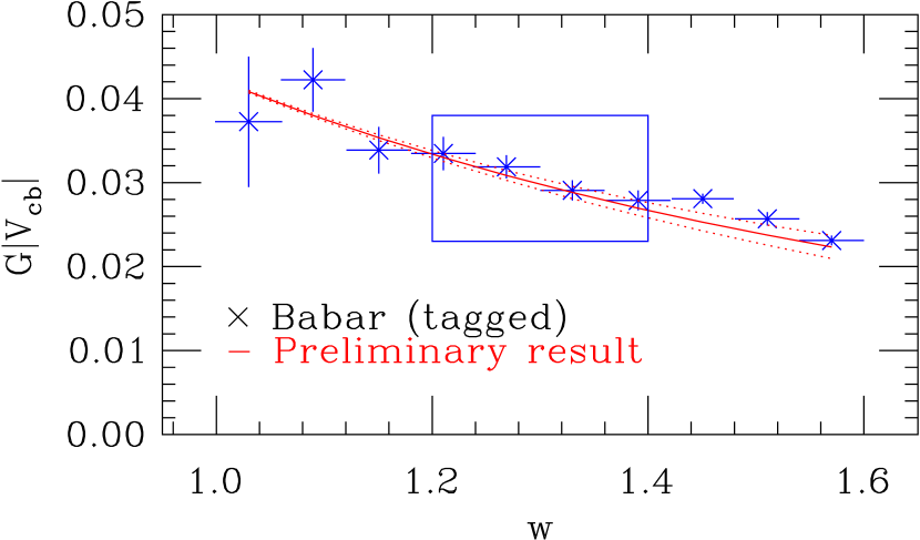
The CKM matrix element $|V_{cb}|$ is a key quantity in Standard-Model tests. It normalizes the legs of the unitarity triangle. The dominant uncertainty in $|V_{cb}|$ comes from theoretical determinations of the hadronic form factors for $B\to c\ell\nu+\ldots{}$. The exclusive processes $B\to D\ell\nu$ and $B\to D^{*}\ell\nu$ [1, 2, 3] can be studied in lattice gauge theory. Here we report on results for $B\rightarrow D\ell\nu$. Lattice calculations at zero recoil typically have the smallest errors. However, because of the phase space suppression near zero recoil in $B\rightarrow D\ell\nu$, experimental errors are largest there. Thus, we aim to work at nonzero recoil where the combined experimental and theoretical error is minimized. This work updates our previous report [4] with all ensembles now included in the analysis.

The differential decay rate $d\Gamma({B}\rightarrow{D}\ell\overline{\nu})/dq^{2}$ is, for $m^{2}_{\ell}\ll\min(M^{2}_{B},q^{2})$, proportional to $|f_{+}|^{2}$ for $\ell=e,\mu$, where for $q=p_{B}-p_{D}$,

$$\langle D(p_{D})|\mathcal{V}^{\mu}|B(p_{B})\rangle=f_{+}(q^{2})\left[(p_{B}+p_{D})^{\mu}-\frac{M_{B}^{2}-M_{D}^{2}}{q^{2}}q^{\mu}\right]+f_{0}(q^{2})\frac{M_{B}^{2}-M_{D}^{2}}{q^{2}}q^{\mu}\,.$$ (1)

Here $\mathcal{V}^{\mu}=\bar{b}\gamma^{\mu}c$ is the $b\to c$ vector current and $f_{+}$ and $f_{0}$ are the vector and scalar form factors, respectively. The alternative form factors $h_{+}$ and $h_{-}$ are convenient:

$$\frac{\langle D(p_{D})|\mathcal{V}^{\mu}|B(p_{B})\rangle}{\sqrt{M_{B}M_{D}}}=h_{+}(w)(v+v^{\prime})^{\mu}+h_{-}(w)(v-v^{\prime})^{\mu}\,,$$ (2)

where $v=p_{B}/M_{B}$ and $v^{\prime}=p_{D}/M_{D}$. They are related to $f_{+}$ and $f_{0}$ through

$$f_{+}(q^{2}) = \frac{1}{2\sqrt{r}}\left[(1+r)h_{+}(w)-(1-r)h_{-}(w)\right]\,,$$

$$f_{0}(q^{2}) = \sqrt{r}\left[\frac{w+1}{1+r}h_{+}(w)-\frac{w-1}{1-r}h_{-}(w)\right],$$ (3)

where $r=M_{D}/M_{B}$ and $q^{2}=M_{B}^{2}+M_{D}^{2}-2wM_{B}M_{D}$ or $w=v\cdot v^{\prime}$.

Figure 1: Left panel: parameters of the 14 lattice ensembles in this study. Plotted are values of the light to strange sea quark mass ratio $m_{\ell}/m_{h}$ vs. the approximate lattice spacing in fm. Right panel: example from the $a=0.06$ fm, $m_{\ell}/m_{h}=0.15$ ensemble with $T=24,25$. Upper curve: the zero-recoil double ratio, middle curve: the ratio $R_{+}({\bf p},t)/R_{+}({\bf 0},t)$ for the 1S smeared $D$-meson interpolator, and bottom curve: the local interpolator. Red points are included in the fit ($p=0.15$).

2 Lattice-QCD calculation

We are carrying out calculations on 14 lattice ensembles generated in the presence of $2+1$ flavors of improved (asqtad) staggered sea quarks [7] with light-quark masses and lattice spacings shown in Fig. 1.

In the $B$ meson rest frame for any recoil $D$-momentum ${\bf p}$ we can obtain $h_{+}$ and $h_{-}$ from matrix elements of the current starting from ratios of lattice matrix elements $R_{+}$ and $R_{-}$, and $x_{f}$, where

$$R_{+}({\bf p}) \equiv \left\langle D({\bf p})|V^{4}|B({\bf 0})\right\rangle$$

$$R_{-}({\bf p}) \equiv \frac{\left\langle D({\bf p})|V^{1}|B({\bf 0})\right\rangle}{\left\langle D({\bf p})|V^{4}|B({\bf 0})\right\rangle}$$

$$x_{f}({\bf p}) \equiv \frac{\left\langle D({\bf p})|V^{1}|D({\bf 0})\right\rangle}{\left\langle D({\bf p})|V^{4}|D({\bf 0})\right\rangle}$$ (4)

$$w({\bf p}) = [1+x_{f}({\bf p})^{2}]/[1-x_{f}({\bf p})^{2}]$$

$$h_{+}(w) = R_{+}({\bf p})[1-x_{f}({\bf p})R_{-}({\bf p})]$$

$$h_{-}(w) = R_{+}({\bf p})[1-R_{-}({\bf p})/x_{f}({\bf p})]\,.$$

At zero recoil, we can also use the double ratio of Hashimoto et al [5]:

$$|h_{+}({\bf 0})|^{2}=\frac{\left\langle D({\bf 0})|V^{1}|B({\bf 0})\right\rangle\left\langle B({\bf 0})|V^{1}|D({\bf 0})\right\rangle}{\left\langle D({\bf 0})|V^{4}|D({\bf 0})\right\rangle\left\langle B({\bf 0})|V^{4}|B({\bf 0})\right\rangle}\,.$$ (5)

The continuum $\mathcal{V}^{\mu}$ and lattice $V^{\mu}$ currents are matched through $\mathcal{V}^{\mu}_{cb}=Z_{V^{\mu}_{cb}}V^{\mu}_{cb}$. We use a mostly nonperturbative method [5], writing

$$Z_{V^{\mu}_{cb}}=\rho_{V^{\mu}_{cb}}\sqrt{Z_{V^{4}_{cc}}Z_{V^{4}_{bb}}}\,,$$ (6)

and determine $\rho_{V^{\mu}_{cb}}$ from one-loop lattice perturbation theory.

In addition to the two-point functions, we need matrix elements $\left\langle Y({\bf p})|V^{\mu}|X(0)\right\rangle$ for $X,Y\in\{B,D\}$. They are constructed from naive light spectator quark propagators and clover heavy quark propagators in the Fermilab interpretation [6] as shown in Fig. 2. Valence bottom and charm quark masses were tuned to the “kinetic” $B_{s}$ and $D_{s}$ masses. The mass of the naive light spectator quark is set equal to that of the light sea quark.

For interpolating operators ${\cal O}_{X}$, we compute two-point and three-point functions

$$C^{2pt,X}({\bf p},t) = \left\langle{\cal O}^{\dagger}_{X}(0){\cal O}_{X}(t)\right\rangle\,,$$ (7)

$$C^{3pt,X\rightarrow Y,\mu}({\bf p};0,t,T) = \left\langle{\cal O}_{Y}^{\dagger}(0)V^{\mu}(t){\cal O}_{X}(T)\right\rangle\,.$$ (8)

We use both point and $1S$ smeared interpolating operators for the $D$ meson and $1S$ smeared interpolating operators for the $B$.

Figure 2: Valence quark line diagram for $B\rightarrow D$.

2.1 Two-point and three-point correlator fits

We obtain the lattice form factors via a two-step procedure. First, we fit the $B$- and $D$-meson two-point correlators to obtain the energies and overlap factors. Then we use these determinations as constraints (with Bayesian priors) in the three-point fits. For illustration, we show the reduction of the three-point and two-point functions to obtain $R_{+}(p)=\left\langle D({\bf p})|V^{4}|B({\bf 0})\right\rangle$. We include excited $B$ and $D$ contributions indicated with a prime but not both together:

$$C_{V4}^{3pt,B\rightarrow D}({\bf p},t) = \sqrt{Z_{D}({\bf p})}\frac{e^{-E_{D}t}}{\sqrt{2E_{D}}}\left\langle D({\bf p})|V^{4}|B({\bf 0})\right\rangle\frac{e^{-m_{B}(T-t)}}{\sqrt{2m_{B}}}\sqrt{Z_{B}({\bf 0})}$$

$$+ \sqrt{Z_{D^{\prime}}({\bf p})}\frac{e^{-E_{D^{\prime}}t}}{\sqrt{2E_{D^{\prime}}}}\left\langle D^{\prime}({\bf p})|V^{4}|B({\bf 0})\right\rangle\frac{e^{-m_{B}(T-t)}}{\sqrt{2m_{B}}}\sqrt{Z_{B}({\bf 0})}$$

$$+ \sqrt{Z_{D}({\bf p})}\frac{e^{-E_{D}t}}{\sqrt{2E_{D}}}\left\langle D({\bf p})|V^{4}|B^{\prime}({\bf p})\right\rangle\frac{e^{-m_{B^{\prime}}(T-t)}}{\sqrt{2m_{B^{\prime}}}}\sqrt{Z_{B^{\prime}}({\bf 0})}\,,$$

or

$$C_{V^{4}}^{3pt,B\rightarrow D}({\bf p},t)=C_{0}({\bf p})\left\langle D({\bf p})|V^{4}|B({\bf 0})\right\rangle e^{-E_{D}t}e^{-m_{B}(T-t)}\left[1+C_{1}({\bf p})e^{-\Delta E_{D}t}+C_{2}({\bf p})e^{(t-T)\Delta m_{B}}\right]\,,$$ (10)

where $C_{0}({\bf p})$, $\Delta E_{D}=E_{D^{\prime}}-E_{D}$, and $\Delta m_{B}=m_{B^{\prime}}-m_{B}$ come from fits to two-point correlators. Terms oscillating as $(-)^{t}$ (not shown) are introduced by the naive light quark. We suppress their contributions by averaging over $T$, $T+1$ and $t$, $t+1$, as introduced in [1].

Putting information from three- and two-point functions together, we get

$$R_{+}({\bf p},t) \equiv \frac{C_{V^{4}}^{3pt,B\rightarrow D}({\bf p},t)e^{(E_{D}-m_{B})t+(m_{B}-m_{D})T/2}}{\sqrt{C_{V^{4}}^{3pt,D\rightarrow D}({\bf 0},t)C_{V^{4}}^{3pt,B\rightarrow B}({\bf 0},t)}}\sqrt{\frac{Z_{D}({\bf 0})E_{D}}{Z_{D}({\bf p})m_{D}}}$$ (11)

$$\approx R_{+}({\bf p})\left[1+s_{1}({\bf p})e^{-\Delta E_{D}t}+s_{2}({\bf p})e^{(t-T)\Delta m_{B}}\right]\,.$$

The zero-recoil form factor $h_{+}({\bf 0})=R_{+}({\bf 0})$ can be calculated very accurately from the double ratio. A good strategy is to use it to normalize the nonzero recoil values:

$$\frac{R_{+}({\bf p},t)}{R_{+}({\bf 0},t)}=\frac{R_{+}({\bf p})}{R_{+}({\bf 0})}\exp(\delta m\,t)+A({\bf p})\exp(-\Delta E_{D}t)+B({\bf p})\exp(\Delta m_{B}t)\,,$$ (12)

where $\delta m=0$, $\Delta E_{D}=E_{D^{\prime}}-E_{D}$, and $\Delta m_{B}=m_{B^{\prime}}-m_{B}$ are constrained by fits to two-point functions.

We do a simultaneous fit to three three-point functions, as illustrated in the right panel of Fig. 1 and determine $R_{+}$, $R_{-}$, and $x_{f}$ for each momentum (recoil parameter $w$), from which we determine $h_{+}$ and $h_{-}$.

Figure 3: Form factors $h_{+}$ (left) and $h_{-}$ (right) as a function of the recoil parameter $w$. The curves in each panel are a result of a simultaneous fit to the chiral-continuum expressions of Eq. (13) with $p=0.68$ for the $h_{+}$ fit and $p=0.41$ for the $h_{-}$ fit.

2.2 Chiral-continuum extrapolation and $q^{2}$ parameterization

The resulting form factors $h_{+}$ and $h_{-}$ are shown in Fig. 3. We fit them to the expressions

$$h_{+}(a,m_{\ell},w) = 1-\rho_{+}^{2}(w-1)+k_{+}(w-1)^{2}+\frac{X_{+}(\Lambda_{\chi})}{m_{c}^{2}}+c_{1,+}m_{\ell}+c_{a,+}a^{2}+c_{a,w,+}a^{2}(w-1)$$ (13)

$$+ \frac{g_{D^{*}D\pi}^{2}}{16\pi^{2}f^{2}}{\rm logs}_{\rm 1-loop}(\Lambda_{\chi},w,m_{\ell},a)$$

$$h_{-}(a,m_{\ell},w) = \frac{X_{-}}{m_{c}}-\rho_{-}^{2}(w-1)+k_{-}(w-1)^{2}+c_{1,-}m_{\ell}+c_{a,-}a^{2}+c_{a,w,-}a^{2}(w-1)$$

for light spectator quark mass $m_{\ell}$, lattice spacing $a$, and $w=v\cdot v^{\prime}$. For the one-loop chiral logs we use a staggered fermion version of Chow and Wise [9]. Thus, these fit functions contain the correct next-to-leading-order chiral perturbation theory expressions, including staggered discretization effects [10]. As can be seen, the dependence of $h_{+}$ on $a$ and $m_{\ell}/m_{h}$ is quite mild. We expect $h_{-}$ to have larger discretization effects than $h_{+}$ because of different HQET power counting. This is consistent with what we see in the data. For $|V_{cb}|$, the contribution coming from $h_{-}$ over the entire kinematic range is small, so the larger errors in $h_{-}$ don’t increase the overall error much. These features with 14 ensembles are consistent with our previous findings with four ensembles [10].

Figure 4: Left: form factors $f_{+}$ and $f_{0}$ parameterized by the $z$ expansion ($p=0.12$). Right: comparison with experimental results from the Babar collaboration [12]. The red line gives our result. The red dotted lines show only statistical errors. The boxed region appears to have the smallest combined error.

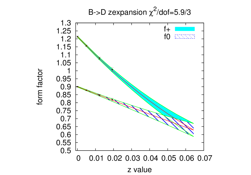
To compare the lattice and experimental form factors we need to extrapolate to larger $w$ (equivalently $q^{2}$). We do this using the $z$-expansion of Boyd, Grinstein and Lebed [11], which provides a model-independent parameterization of the $q^{2}$ dependence of $f_{+}$ and $f_{0}$. This expansion builds in constraints from analyticity and unitarity. It is based on the conformal map

$$z(w)=\frac{\sqrt{1+w}-\sqrt{2}}{\sqrt{1+w}+\sqrt{2}}\,,$$ (14)

which maps the physical region $w\in[1,1.59]$ to $z\in[0,0.0644]$. It pushes poles and branch cuts far away at $|z|\approx 1$. Form factors are then parameterized as

$$f_{i}(z)=\frac{1}{P_{i}(z)\phi_{i}(z)}\sum_{n=0}^{\infty}a_{i,n}z^{n}\,,$$ (15)

where $P_{i}(z)$ are the Blaschke factors and $\phi_{i}$ are the “outer functions”. The latter are chosen to simplify the unitarity bound:

$$\sum_{n}|a_{i,n}|^{2}\leq 1\,.$$ (16)

In practice, we need only the first few coefficients in the expansion. We also impose the kinematic constraint $f_{+}=f_{0}$ at $q^{2}=0$ or $z\approx 0.0644$.

To implement the $z$ expansion, we start from the value of $f_{+}$ and $f_{0}$ at the physical point, as determined from the chiral/continuum fit. We choose four $w$ values, $w=1.00$, 1.04, 1.10, and 1.16, and use the corresponding form factor values to determine the coefficients $a_{i,0}$, $a_{i,1}$, and $a_{i,2}$. These, then, are used to parameterize the form factors over the full kinematic range, as shown in the left panel of Fig. 4.

We compare our result with experimental measurements from the Babar collaboration [12] in Fig. 4. For present purposes we take $|V_{cb}|$ from $B\to D^{*}\ell\nu$ at zero recoil [3].

3 Future plans

To complete the analysis, we need to apply small corrections resulting from adjusting the charm and bottom quark masses to their tuned values, implement the full current renomalization, and compile a complete error budget.

References

- [1] C. Bernard et al. [Fermilab Lattice and MILC Collaborations], Phys. Rev. D79 014506 (2009). [arXiv:0808.2519 [hep-lat]].
- [2] J. Laiho, R. S. Van de Water, Phys. Rev. D73, 054501 (2006). [hep-lat/0512007].
- [3] J. A. Bailey et al. [Fermilab Lattice and MILC Collaborations], \posPoS(Lattice 2010)311 (2010) [arXiv:1011.2166 [hep-lat]].
- [4] Si-Wei Qiu et al. [Fermilab Lattice and MILC Collaborations], \posPoS(Lattice 2011)289 (2011) [arXiv:1111.0677 [hep-lat]].
- [5] S. Hashimoto, A. S. Kronfeld, P. B. Mackenzie, S. M. Ryan, and J. N. Simone, Phys. Rev. D66, 014503 (2002). [hep-ph/0110253]; J. Harada, S. Hashimoto, A. S. Kronfeld, and T. Onogi, Phys. Rev. D 65, 094514 (2002) [hep-lat/0112045].
- [6] A. X. El-Khadra, A. S. Kronfeld, P. B. Mackenzie, Phys. Rev. D55, 3933-3957 (1997). [hep-lat/9604004].
- [7] T. Blum et al. [MILC Collaboration], Phys. Rev. D 55, 1133 (1997) [hep-lat/9609036]. C. W. Bernard et al. [MILC Collaboration], Phys. Rev. D 58, 014503 (1998) [hep-lat/9712010]. K. Orginos et al. [MILC Collaboration], Phys. Rev. D 59, 014501 (1999) [hep-lat/9805009]. J. F. Lagaë and D. K. Sinclair, Phys. Rev. D 59, 014511 (1999) [hep-lat/9806014]. G. P. Lepage, Phys. Rev. D 59, 074502 (1999) [hep-lat/9809157]. K. Orginos et al. [MILC Collaboration], Phys. Rev. D 60, 054503 (1999) [hep-lat/9903032].
- [8] A. Bazavov et al., Rev. Mod. Phys. 82, 1349 (2010) [arXiv:0903.3598 [hep-lat]].
- [9] C. K. Chow and M. B. Wise, Phys. Rev. D 48 (1993) 5202 [arXiv:hep-ph/9305229].
- [10] J. A. Bailey et al., Phys. Rev. D 85, 114502 (2012) [Erratum-ibid. D 86, 039904 (2012)] [arXiv:1202.6346 [hep-lat]].
- [11] C. G. Boyd, B. Grinstein and R. F. Lebed, Phys. Rev. Lett. 74, 4603 (1995) [hep-ph/9412324].
- [12] B. Aubert et al. [BABAR Collaboration], Phys. Rev. Lett. 104, 011802 (2010) [arXiv:0904.4063 [hep-ex]].