Systematic approach to thermal leptogenesis

Abstract

In this work we study thermal leptogenesis using non-equilibrium quantum field theory. Starting from fundamental equations for correlators of the quantum fields we describe the steps necessary to obtain quantum kinetic equations for quasiparticles. These can easily be compared to conventional results and overcome conceptional problems inherent in the canonical approach. Beyond CP-violating decays we include also those scattering processes which are tightly related to the decays in a consistent approximation of fourth order in the Yukawa couplings. It is demonstrated explicitly how the S-matrix elements for the scattering processes in the conventional approach are related to two- and three-loop contributions to the effective action. We derive effective decay and scattering amplitudes taking medium corrections and thermal masses into account. In this context we also investigate CP-violating Higgs decay within the same formalism. From the kinetic equations we derive rate equations for the lepton asymmetry improved in that they include quantum-statistical effects and medium corrections to the quasiparticle properties.

I Introduction

If one combines today’s Standard Model of particle physics (SM) and that of cosmology, one finds inevitably that particles and their antiparticles annihilate at a very early moment in the evolution of the universe, leaving just radiation behind. The absence of a sizable matter-antimatter asymmetry at this epoch would imply that the universe as we know it could never form. The question about the origin of the observed asymmetry therefore represents a major challenge for modern physics.

In the SM baryon and lepton number are (accidental) global symmetries. If baryon number was also conserved in the early Universe a dynamical emergence of the asymmetry would have been impossible. In grand-unified extensions (GUTs) of the SM baryon number (and also lepton number) is explicitly broken. According to past reasoning, this could provide a solution to the apparent discrepancy. In the class of ‘GUT-baryogenesis’ scenarios the matter-antimatter imbalance is generated by asymmetric decays of new super-heavy bosons. Anomalous electroweak processes ’t Hooft (1976); Klinkhamer and Manton (1984) (sphalerons) which violate baryon and lepton number but conserve their difference essentially eliminated the prospects for GUT-baryogenesis Kuzmin et al. (1985). At the same time, it inspired the now widely appreciated scenarios of ‘electroweak baryogenesis’ Kuzmin et al. (1985); Morrissey and Ramsey-Musolf (2012) and ‘baryogenesis via leptogenesis’ Fukugita and Yanagida (1986). According to the latter scenario, the asymmetry is initially generated in the leptonic sector by the decay of heavy Majorana neutrinos at an energy scale far above the electroweak scale. Subsequently it is converted into the observed baryon asymmetry by sphalerons. The mass scale of the heavy Majorana neutrinos required for leptogenesis Davidson and Ibarra (2002); Hamaguchi et al. (2002) fits together very well with the mass-differences inferred from observations of solar-, atmospheric- and reactor-neutrino oscillations.

We focus here on the conventional, but most popular, high-energy (type-I) seesaw extension:

$$\mathscr{L}=\mathscr{L}_{SM} +{\textstyle\frac{1}{2}}\bar{N}_{i}\bigl{(}i\displaystyle{\not}\partial-M_{i}\bigr{)}N_{i}$$

$$-h_{\alpha i}\bar{\ell}_{\alpha}{\tilde{\phi}}P_{R}N_{i}-h^{\dagger}_{i\alpha}\bar{N}_{i}{\tilde{\phi}}^{\dagger}P_{L}{\ell}_{\alpha}{\,,}$$ (1)

where $N_{i}=N^{c}_{i}$ are the heavy Majorana fields, ${\ell}_{\alpha}$ are the lepton doublets, $\tilde{\phi}\equiv i\sigma_{2}\phi^{*}$ is the conjugate of the Higgs doublet, and $h$ are the corresponding Yukawa couplings. The Majorana mass term violates lepton number and the Yukawa couplings can violate CP. Therefore the model fulfills essential requirements for baryogenesis Sakharov (1967). They can also be realized for more complicated SM extensions and a wide range of values for couplings and neutrino masses Buchmüller et al. (2005a); Giudice et al. (2004); Davidson et al. (2008); Blanchet and Di Bari (2012). In general the right-handed neutrinos do not necessarily get into thermal equilibrium and CP-violating oscillations between them can contribute to the asymmetry. This effect of leptogenesis through neutrino oscillations Akhmedov et al. (1998) is crucial for neutrino-minimal extensions of the SM ($\nu$MSM) Canetti et al. (2012) and poses interesting questions for non-equilibrium quantum field theory Garny et al. (2011); Garbrecht and Herranen (2012); Drewes and Garbrecht (2012). In the considered scenario of thermal leptogenesis the heavy Majorana neutrinos experience only a moderate deviation from thermal equilibrium at the time when the bulk of the asymmetry is produced. Also, for a hierarchical mass spectrum, effects related to oscillations are negligible.

The amount of the generated asymmetry is determined by the out of equilibrium evolution of the heavy Majorana neutrinos. Therefore, statistical equations for the abundance of the neutrinos and the generated asymmetry are needed. The conventional approach here follows the lines developed for GUT-baryogenesis Kolb and Turner (1990). The CP-violating amplitudes for the decay and scattering processes involving the heavy Majorana neutrinos are computed in terms of Feynman graphs at lowest loop order. They are used to build generalized Boltzmann collision terms for these processes. Each of them contributes to the evolution of the distributions of Majorana neutrinos and leptons or, upon momentum integration, their entire abundances.

However this approach is plagued by the so-called double-counting problem which manifests itself in the generation of a non-vanishing asymmetry even in thermal equilibrium. This technical issue is expression of the fact that the ‘naive’ generalization of the collision terms is quantitatively inexact, and inconsistent in the presence of CP-violation. After a real intermediate state (or RIS) subtraction procedure and a number of approximations, it can be made consistent with fundamental requirements. Nevertheless this pragmatic solution remains unsatisfactory. The requirement of unitarity guarantees a consistent approximation for the amplitudes, realized by the RIS subtraction, if the statistical system is in thermal equilibrium. However, the deviation from equilibrium is a fundamental requirement for leptogenesis and it is not obvious how the equations have to be generalized for a system out of equilibrium.

Furthermore, the CP-violation arises from one-loop contributions due to the exchange of virtual quanta. As such they seem to be beyond a Boltzmann approximation. But the relevant imaginary part is due to intermediate states in which at least some of the particles are on-shell. These can also be absorbed or emitted by the medium and it is not obvious how such contributions enter the amplitudes. It is, however, clear that the influence of medium effects on the one-loop contributions enters directly the CP-violating parameter and therefore the source for the lepton asymmetry. Their size can be of the same order as that of the vacuum contributions.

Those questions can be addressed within a first-principle approach based on non-equilibrium quantum field theory (NEQFT). Several aspects of leptogenesis have already been investigated within this approach Buchmüller and Fredenhagen (2000). The influence of medium effects on the generation of the asymmetry has been studied e.g. in Garny et al. (2009, 2010a, 2010b); Beneke et al. (2010); Garny et al. (2010c); Garbrecht (2011); Drewes and Garbrecht (2012), and an analysis with special emphasis on off-shell effects was performed in Anisimov et al. (2010a, b). The role of flavor effects as well as the range of applicability of the conventional approach to the analysis of flavored leptogenesis has been investigated in Beneke et al. (2011). The resonant enhancement of the lepton asymmetry has been addressed within a first-principle approach in Garny et al. (2011); Garbrecht and Herranen (2012); Garbrecht (2012a, b). In addition, steps towards a consistent inclusion of gauge interactions have been taken Giudice et al. (2004); Kießig and Plümacher (2012a, b); Besak and Bodeker (2010); Anisimov et al. (2011); Laine and Schroder (2012); Salvio et al. (2011); Besak and Bodeker (2012).

In this work we use the 2PI-formalism of NEQFT to derive Boltzmann-like quantum kinetic equations for the lepton asymmetry. In particular, we show how two-body scattering processes that violate lepton number by two units and contribute to the washout of the asymmetry emerge within the 2PI-formalism. This approach treats quantum field theory and the out of equilibrium evolution on an equal footing and allows to overcome the conceptional difficulties inherent in the conventional approach. It allows us to obtain quantum-generalized Boltzmann equations which include medium effects and which are free of the double-counting problem. In other words, the structure of the obtained quantum kinetic equations automatically ensures that the asymmetry vanishes in thermal equilibrium and no need for RIS subtraction arises. The resulting equation for the lepton asymmetry $Y_{L}$ is given by

$$\frac{s{\cal H}}{z}\frac{dY_{L}}{dz} =\sum_{i}\int{\,d\Pi_{{\ell}\phi N_{i}}^{pkq}}{\mathcal{F}_{{\ell}\phi\leftrightarrow N_{i}}^{pk;q}}\Xi_{{\ell}\phi\leftrightarrow N_{i}}$$

$$-\sum_{i}\int{\,d\Pi_{\bar{\ell}\bar{\phi}N_{i}}^{pkq}}{\mathcal{F}_{\bar{\ell}\bar{\phi}\leftrightarrow N_{i}}^{pk;q}}\Xi_{\bar{\ell}\bar{\phi}\leftrightarrow N_{i}}$$

$$-2\int{\,d\Pi_{{\ell}\phi\bar{\ell}\bar{\phi}}^{p_{1}k_{1}p_{2}k_{2}}}{\mathcal{F}_{\bar{\ell}\bar{\phi}\leftrightarrow{\ell}\phi}^{p_{2}k_{2};p_{1}k_{1}}}\Xi_{\bar{\ell}\bar{\phi}\leftrightarrow{\ell}\phi}$$

$$-\int{\,d\Pi_{{\ell}{\ell}\bar{\phi}\bar{\phi}}^{p_{1}p_{2}k_{1}k_{2}}}{\mathcal{F}_{\bar{\phi}\bar{\phi}\leftrightarrow{\ell}{\ell}}^{k_{1}k_{2};p_{1}p_{2}}}\Xi_{\bar{\phi}\bar{\phi}\leftrightarrow{\ell}{\ell}}$$

$$-\int{\,d\Pi_{\bar{\ell}\bar{\ell}\phi\phi}^{p_{1}p_{2}k_{1}k_{2}}}{\mathcal{F}_{\bar{\ell}\bar{\ell}\leftrightarrow\phi\phi}^{p_{1}p_{2};k_{1}k_{2}}}\Xi_{\bar{\ell}\bar{\ell}\leftrightarrow\phi\phi}{\,.}$$ (2)

Together with the ‘effective amplitudes’ $\Xi$ this is the main result of this paper. In Eq. (2) we introduced

$${\mathcal{F}_{ab..\leftrightarrow ij..}^{p_{a}p_{b}..;p_{i}p_{j}..}} \equiv(2\pi)^{4}\delta(p_{a}+p_{b}+..-p_{i}-p_{j}-..)$$

$$\times\bigl{[}f_{i}f_{j}..(1-\xi^{a}f_{a})(1-\xi^{b}f_{b})..$$

$$-f_{a}f_{b}..(1-\xi^{i}f_{i})(1-\xi^{j}f_{j})..\bigr{]}{\,,}$$ (3)

with $\xi^{a}=+(-)1$ for fermions (bosons). Note that ${\mathcal{F}_{ab..\leftrightarrow ij..}^{p_{a}p_{b}..;p_{i}p_{j}..}}$ vanishes in equilibrium due to detailed balance. This ensures that the asymmetry vanishes in thermal equilibrium as mentioned before. The effective amplitudes contain medium effects ignored in the corresponding canonical expressions.

We find that, in the amplitudes of the scattering processes medium effects are sub-dominant and can be neglected. The total decay amplitude of the Majorana neutrino is barely affected as well. However, at high temperatures the available phase space shrinks when taking gauge interactions in the form of effective thermal masses of Higgs and leptons into account. This leads to a suppression of the decay and scattering rates. Since the CP-violation appears as loop effect it is more sensitive to influences of the surrounding medium. Even though there is a partial cancellation of the fermionic and bosonic contributions, the CP-violating parameter is enhanced by medium effects. However, the thermal masses reduce the enhancement and turn it into suppression at high temperatures.

We review the conventional approach to leptogenesis based on RIS subtraction in Sec. II. In section III we demonstrate explicitly that in thermal equilibrium the success of this procedure is guaranteed by the requirement of unitarity. In Sec. IV we review the derivation of rate equations for total abundances and discuss in how far quantum statistical and medium corrections can be incorporated in the reaction densities. In Sec. V we review the application of the 2PI approach of NEQFT to leptogenesis. Equation (2) and explicit expressions for the effective in-medium decay and scattering amplitudes are derived within this framework in Sec. VI. We compare the results obtained within the 2PI-formalism to those of a conventional analysis with manual RIS subtraction. In Sec. VII we derive rate equations and the CP-violating amplitudes for Higgs decay within the framework of NEQFT. Finally, we summarize the results and present our conclusions in Sec. VIII.

II Conventional approach

The amount of produced asymmetry depends on the details of the non-equilibrium evolution of the Majorana neutrinos as well as on the strength of CP-violation. The latter is usually quantified by CP-violating parametersBuchmüller et al. (2005a); Giudice et al. (2004); Davidson et al. (2008); Blanchet and Di Bari (2012):

$$\epsilon_{i}\equiv\frac{\Gamma_{N_{i}\rightarrow{\ell}\phi}-\Gamma_{N_{i}\rightarrow\bar{\ell}\bar{\phi}}}{\Gamma_{N_{i}\rightarrow{\ell}\phi}+\Gamma_{N_{i}\rightarrow\bar{\ell}\bar{\phi}}}{\,,}$$

where $\Gamma_{N_{i}\rightarrow{\ell}\phi}$ and $\Gamma_{N_{i}\rightarrow\bar{\ell}\bar{\phi}}$ are the vacuum decay rates to a particle or anti-particle pair respectively.For a hierarchical mass spectrum $\epsilon_{i}$ can be computed perturbatively as the interference

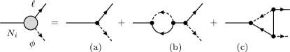
Figure 1: Tree-level, one-loop self-energy and one-loop vertex contributions to the decay of the heavy Majorana neutrino.

of the tree-level, one-loop vertex Fukugita and Yanagida (1986) and one-loop self-energy Flanz et al. (1995); Covi et al. (1996); Pilaftsis (1997) amplitudes in Fig. 1. The contribution of the loop diagrams can be accounted for by effective Yukawa couplings Pilaftsis and Underwood (2004):

$$\lambda_{+,\alpha i} \equiv h_{\alpha i}-ih_{\alpha j}(h^{\dagger}h)^{*}_{ji}\,f_{ij}{\,,}$$ (4a)

$$\lambda_{-,\alpha i} \equiv h^{*}_{\alpha i}-ih^{*}_{\alpha j}(h^{\dagger}h)_{ji}\,f_{ij}{\,,}$$ (4b)

where the loop function $f_{ij}$ is defined as

$$f_{ij}\equiv \frac{1}{16\pi}\frac{M_{i}M_{j}}{M^{2}_{i}-M^{2}_{j}}$$ (5)

$$+ \frac{1}{16\pi}\frac{M_{j}}{M_{i}}\biggl{[}1-\biggl{(}1+\frac{M_{j}^{2}}{M_{i}^{2}}\biggr{)}\ln\biggl{(}1+\frac{M_{i}^{2}}{M_{j}^{2}}\biggr{)}\biggr{]}{\,.}$$

The first term in Eq. (5) is related to the self-energy and the second term to the vertex contribution. The decay widths are proportional to the absolute values of the effective couplings, $\Gamma_{N_{i}\rightarrow{\ell}\phi}=g_{w}(\lambda^{\dagger}_{+}\lambda^{\phantom{\dagger}}_{+})_{ii}M_{i}/(32\pi)$ and $\Gamma_{N_{i}\rightarrow\bar{\ell}\bar{\phi}}=g_{w}(\lambda^{\dagger}_{-}\lambda^{\phantom{\dagger}}_{-})_{ii}M_{i}/(32\pi)$ respectively, where we have summed over flavors of the leptons and $SU(2)_{L}$ indices (hence the factor $g_{w}=2$) in the final state. Since the phase space for the decay into particles and antiparticles is the same, one gets for the CP-violating parameter:

$$\epsilon^{vac}_{i}\approx\frac{\Im(h^{\dagger}h)^{2}_{ij}}{(h^{\dagger}h)_{ii}}\times 2f_{ij}{\,,}\quad j\neq i{\,.}$$ (6)

Let us note in passing that the divergence of the loop function for $j=i$ is not physical and can be removed by a resummation of the self-energy contribution Pilaftsis (1997); Plümacher (1998); Pilaftsis and Underwood (2004). Here we work in a regime where the mass splittings $\left|M_{i}-M_{j}\right|$ are large enough to render effects related to the enhancement of the self-energy contribution irrelevant (non-resonant leptogenesis). We do not require a strictly hierarchical mass-spectrum, however.

To describe the statistical evolution of the lepton asymmetry one usually employs generalized Boltzmann equations for the one-particle distribution functions of the different species Kolb and Wolfram (1980); Bernstein (1988); Kolb and Turner (1990). Taking into account decay and inverse decay processes one writes for the distribution function of the leptons (for a single flavor):

$$p^{\mu}{\cal D}_{\mu}f_{{\ell}} =\frac{1}{2}\sum_{i,s_{i}}\int\,d\Pi^{\phi}_{k}\,d\Pi^{{N_{i}}}_{q}(2\pi)^{4}\delta(p+k-q)$$

$$\times\bigl{[}\left|\mathcal{M}\right|_{{{N_{i}}}\rightarrow{{\ell}\phi}}^{2}(1-f_{{\ell}})(1+f_{\phi})f_{N_{i}}$$

$$-\left|\mathcal{M}\right|_{{{\ell}\phi}\rightarrow{{N_{i}}}}^{2}f_{{\ell}}f_{\phi}(1-f_{N_{i}})\bigr{]}{\,,}$$ (7)

where $\,d\Pi^{a}_{p}=d^{3}p/[(2\pi)^{3}2E_{p}]$ is the invariant phase space element, $s_{i}$ denotes spin degrees of freedom of $N_{i}$, and ${\cal D}_{\mu}$ is the covariant derivative. The corresponding equation for antileptons may be obtained by interchanging ${\ell}\leftrightarrow\bar{{\ell}}$ and $\phi\leftrightarrow\bar{\phi}$. CPT-invariance implies that $\left|\mathcal{M}\right|_{N_{i}\rightarrow{\ell}\phi}^{2}=\left|\mathcal{M}\right|_{\bar{\ell}\bar{\phi}\rightarrow N_{i}}^{2}$ and $\left|\mathcal{M}\right|_{N_{i}\rightarrow\bar{\ell}\bar{\phi}}^{2}=\left|\mathcal{M}\right|_{{\ell}\phi\rightarrow N_{i}}^{2}$. Furthermore, in thermal equilibrium detailed balance requires that $(1-{f}_{{\ell}}^{eq})(1-{f}_{\phi}^{eq}){f}_{N_{i}}^{eq}={f}_{{\ell}}^{eq}{f}_{\phi}^{eq}(1-{f}_{N_{i}}^{eq})$. Subtracting the two relations we find for the contribution of the (inverse) decay terms:

$$p^{\mu}{\cal D}_{\mu}(f_{{\ell}}-f_{\bar{\ell}})=2\cdot\frac{1}{2}\sum_{i,s_{i}}\int\,d\Pi^{\phi}_{k}\,d\Pi^{{N_{i}}}_{q}(2\pi)^{4}\delta(p+k-q)$$

$$\times{f}_{N_{i}}^{eq}(1-{f}_{{\ell}}^{eq})(1+{f}_{\phi}^{eq})\bigl{[}\left|\mathcal{M}\right|_{N_{i}\rightarrow{\ell}\phi}^{2}-\left|\mathcal{M}\right|_{N_{i}\rightarrow\bar{\ell}\bar{\phi}}^{2}\bigr{]}{\,.}$$ (8)

If the decay amplitudes in square brackets differ, the right-hand side of Eq. (II) represents the (non-zero) CP-violating source term for the asymmetry generation. The total asymmetry is given by the sum over all flavors and $SU(2)_{L}$ components: $n_{L}\equiv\sum_{\alpha,a}(n_{\ell}-n_{\bar{\ell}})$. Neglecting the quantum-statistical terms, $(1-f_{{\ell}})(1+f_{\phi})\approx 1$, and integrating Eq. (II) over the lepton phase space we obtain for its time derivative:

$$\partial_{t}n_{L} \approx 2\cdot\frac{g_{N}}{2\pi^{2}}\,\sum_{i}\epsilon_{i}\,\Gamma_{i}\,M_{i}^{2}\,T\,K_{1}\left(\frac{M_{i}}{T}\right)\neq 0{\,,}$$ (9)

where $K_{1}$ is the modified Bessel function of the second kind, $\Gamma_{i}=\Gamma_{N_{i}\rightarrow{\ell}\phi}+\Gamma_{N_{i}\rightarrow\bar{\ell}\bar{\phi}}$ is the total tree-level decay width of $N_{i}$, and the factor $g_{N}=2$ emerges from the sum over the Majorana spin degrees of freedom in (II), see Appendix A for more details. This implies that the source-term for the lepton asymmetry differs from zero even in equilibrium. On the other hand, combined with time translational invariance of an equilibrium state, CPT-invariance requires the asymmetry to vanish in thermal equilibrium. Thus, we arrive at an apparent contradiction.

The generation of an asymmetry in equilibrium within the $S$-matrix formalism is a manifestation of the so-called double-counting problem. In vacuum an inverse decay immediately followed by a decay is equivalent to a scattering process where the intermediate particle is on the mass shell (real intermediate state or RIS).

Figure 2: Two-body scattering process $\bar{\ell}\bar{\phi}\leftrightarrow{\ell}\phi$. Both graphs contribute with all $N_{i}$ as intermediate states. Note that we read (b) as t-channel contribution.

Thus, the same contribution is taken into account twice: once by the amplitude for (inverse) decay processes, and once by that for the ${\ell}\phi\leftrightarrow\bar{\ell}\bar{\phi}$ scattering processes, see Fig. 2.(a).

Let us convince ourselves that this is indeed the case. Including scattering processes we have for the distribution function of the leptons:

$$p^{\mu}{\cal D}_{\mu}f_{{\ell}} =\ldots$$

$$+\frac{1}{2}\sum_{\alpha,a}\int{\,d\Pi_{\bar{\ell}\bar{\phi}\phi}^{p_{2}k_{2}k_{1}}}(2\pi)^{4}\delta(p+k_{1}-p_{2}-k_{2})$$

$$\times\bigl{[}\left|\mathcal{M}\right|_{{\bar{\ell}\bar{\phi}}\rightarrow{{\ell}\phi}}^{2}f_{\bar{\ell}}f_{\bar{\phi}}(1-f_{{\ell}})(1+f_{\phi})$$

$$-\left|\mathcal{M}\right|_{{{\ell}\phi}\rightarrow{\bar{\ell}\bar{\phi}}}^{2}f_{{\ell}}f_{\phi}(1-f_{\bar{\ell}})(1+f_{\bar{\phi}})\bigr{]}{\,,}$$ (10)

where the dots denote the contribution of the (inverse) decay processes, the sum is over flavors and $SU(2)_{L}$ components of the antileptons and we have introduced

$${\,d\Pi_{ab\dotso ij\dotso}^{p_{a}p_{b}\dotso p_{i}p_{j}\dotso}}\equiv \,d\Pi^{a}_{p_{a}}\,d\Pi^{b}_{p_{b}}\ldots\,d\Pi^{i}_{p_{i}}\,d\Pi^{j}_{p_{j}}\ldots{\,,}$$ (11)

to shorten the notation. In the unflavored regime, to which we restrict our analysis, the distribution functions of leptons of all flavors are equal. If the Majorana neutrinos are close to equilibrium the difference between the distribution functions of the two spin degrees of freedom can be neglected as well. Therefore, in the expression for the total asymmetry $n_{L}$ the summation over spin, flavor and $SU(2)_{L}$ components reduces to summation of the corresponding decay and scattering amplitudes. We will denote these sums over internal degrees of freedom by $\Xi$ and call them effective amplitudes in the following. For the effective amplitude of $\bar{\ell}\bar{\phi}\rightarrow{\ell}\phi$ scattering one obtains Pilaftsis and Underwood (2004)

$$\Xi_{\bar{\ell}\bar{\phi}\rightarrow{\ell}\phi} =4(p_{1}p_{2})\textstyle\sum_{ij}M_{i}M_{j}$$ (12)

$$\times\big{[}2(\lambda^{\dagger}_{+}\lambda^{\phantom{\dagger}}_{+})^{2}_{ij}\,P^{*}_{i}(s)P_{j}(s)+2(h^{\dagger}h)^{2}_{ij}\,P^{*}_{i}(t)P_{j}(t)$$

$$+(\lambda_{+}^{\dagger}h)^{2}_{ij}\,P^{*}_{i}(s)P_{j}(t)+(h^{\dagger}\lambda_{+})^{2}_{ij}\,P^{*}_{i}(t)P_{j}(s)\big{]}{\,,}$$

where $p_{1,2}$ are the momenta of initial and final leptons respectively, and $s$ and $t$ are the usual Mandelstam variables. The amplitude $\Xi_{{\ell}\phi\rightarrow\bar{\ell}\bar{\phi}}$ is obtained by interchanging $\lambda_{+}\leftrightarrow\lambda_{-}$. Note that the loop corrections to the Yukawas vanish for negative momentum transfer, i.e. in the $t$-channel. For this reason the above scattering amplitude contains combinations of the Yukawa couplings and their one-loop corrected counterparts. The propagators $P_{i}$ are given by

$$P^{-1}_{i}(q^{2})=q^{2}-M_{i}^{2}+i\theta(q^{2})M_{i}\Gamma_{i}{\,,}$$ (13)

where $\theta$ is the Heaviside step function. The RIS contribution appears for the flavor diagonal ($i=j$) terms in the product of the $s$-channel amplitudes since only in this case the $s-M^{2}_{i}$ terms vanish simultaneously in both $P_{i}$ and $P_{j}$. In other words:

$$\Xi_{\bar{\ell}\bar{\phi}\rightarrow N_{i}\rightarrow{\ell}\phi}=\frac{8(\lambda^{\dagger}_{+}\lambda^{\phantom{\dagger}}_{+})^{2}_{ii}M_{i}^{2}(p_{1}p_{2})}{(s-M_{i}^{2})^{2}+(M_{i}\Gamma_{i})^{2}}{\,,}$$ (14)

and a similar result for $\Xi_{{\ell}\phi\rightarrow N_{i}\rightarrow\bar{\ell}\bar{\phi}}$. Using the definitions of the effective couplings (4) and the expression for the CP-violating parameter (6) we find that $(\lambda^{\dagger}_{+}\lambda^{\phantom{\dagger}}_{+})^{2}\approx(h^{\dagger}h)^{2}_{ii}\,(1+\epsilon_{i})^{2}$. Furthermore, for a small decay width, we can approximate the Breit-Wigner propagator by a delta-function using,

$$\lim\limits_{\epsilon\rightarrow 0+}\frac{2\epsilon}{\omega^{2}+\epsilon^{2}}=\lim\limits_{\epsilon\rightarrow 0+}\frac{4\epsilon^{3}}{[\omega^{2}+\epsilon^{2}]^{2}}=2\pi\delta(\omega){\,,}$$ (15)

where $\omega=s-M_{i}^{2}$ and $\epsilon_{i}=M_{i}\Gamma_{i}$ in the considered case. The RIS contribution to the scattering amplitude then takes the form

$$\Xi_{\bar{\ell}\bar{\phi}\rightarrow N_{i}\rightarrow{\ell}\phi} \approx\Xi_{\bar{\ell}\bar{\phi}\rightarrow N_{i}}\frac{\pi\delta(s-M_{i}^{2})}{M_{i}\Gamma_{i}}\Xi_{N_{i}\rightarrow{\ell}\phi}$$

$$\times\frac{2(p_{1}p_{2})}{M_{i}^{2}}{\,,}$$ (16)

where $\Xi_{N_{i}\rightarrow{\ell}\phi}=g_{w}(\lambda^{\dagger}_{+}\lambda^{\phantom{\dagger}}_{+})_{ii}2pq\approx g_{w}(\lambda^{\dagger}_{+}\lambda^{\phantom{\dagger}}_{+})_{ii}M_{i}^{2}$ is the decay amplitude squared summed over all internal degrees of freedom (and a similar expression for anti-particles). Just as one would expect, it is proportional to the product of the corresponding inverse decay and decay amplitudes. The additional momentum dependence (momenta of the leptons) arises because the initial and final states contain fermions. Close to thermal equilibrium $f_{\bar{\ell}}\approx f_{{\ell}}\approx{f}_{{\ell}}^{eq}$ and $f_{\bar{\phi}}\approx f_{\phi}\approx{f}_{\phi}^{eq}$. Neglecting the quantum-statistical terms we can write the RIS contribution to the source-term as:

$$\partial_{t}n_{L} \approx 2\int{\,d\Pi_{\bar{\ell}\bar{\phi}{\ell}\phi}^{p_{1}k_{1}p_{2}k_{2}}}(2\pi)^{4}\delta(p_{1}+k_{1}-p_{2}-k_{2})$$

$$\times{f}_{{\ell}}^{eq}{f}_{\phi}^{eq}\,\bigl{[}\Xi_{\bar{\ell}\bar{\phi}\rightarrow N_{i}\rightarrow{\ell}\phi}-\Xi_{{\ell}\phi\rightarrow N_{i}\rightarrow\bar{\ell}\bar{\phi}}\,\bigr{]}{\,.}$$ (17)

Taking into account that with Maxwell-Boltzmann distributions ${f}_{{\ell}}^{eq}{f}_{\phi}^{eq}={f}_{N_{i}}^{eq}$ in the presence of the Dirac-delta and performing the phase space integration using Eq. (164) we obtain a result identical to Eq. (9).

To correct the double-counting in equilibrium we may therefore subtract the RIS contribution from the scattering amplitude:

$$\Xi^{{}^{\prime}}_{\bar{\ell}\bar{\phi}\rightarrow{\ell}\phi}\equiv\Xi_{\bar{\ell}\bar{\phi}\rightarrow{\ell}\phi}-\Xi_{\bar{\ell}\bar{\phi}\rightarrow N_{i}\rightarrow{\ell}\phi}{\,,}$$ (18)

and similarly for the conjugate process ${\ell}\phi\rightarrow\bar{\ell}\bar{\phi}$. At first sight it might seem that the RIS subtracted scattering amplitudes $\Xi^{{}^{\prime}}$ do not contribute to the generation of the lepton asymmetry in equilibrium,

$$\partial_{t}n_{L} \approx 2\int{\,d\Pi_{\bar{\ell}\bar{\phi}{\ell}\phi}^{p_{1}k_{1}p_{2}k_{2}}}(2\pi)^{4}\delta(p_{1}+k_{1}-p_{2}-k_{2})$$

$$\times{f}_{{\ell}}^{eq}{f}_{\phi}^{eq}\,\bigl{[}\Xi_{\bar{\ell}\bar{\phi}\rightarrow{\ell}\phi}-\Xi_{\bar{\ell}\bar{\phi}\rightarrow N_{i}\rightarrow{\ell}\phi}$$

$$\hskip 48.36967pt-\Xi_{{\ell}\phi\rightarrow\bar{\ell}\bar{\phi}}+\Xi_{{\ell}\phi\rightarrow N_{i}\rightarrow\bar{\ell}\bar{\phi}}\,\bigr{]}{\,,}$$ (19)

but also cannot compensate the asymmetry generated in equilibrium by the decay processes, see Eq. (9). However, upon phase space integration the difference of the unsubtracted scattering amplitudes vanishes at leading order in $h$. The remaining difference of the RIS-amplitudes precisely compensates the contribution of the (inverse) decay processes (9).

The RIS subtracted scattering amplitude can be conveniently rewritten in terms of a ‘RIS subtracted propagator’ ${\cal P}_{ij}$. Motivated by Eq. (15) we define its diagonal components such, that they vanish upon integration over $s$ in the vicinity of the mass pole:

$${\cal P}_{ii}(s)=\frac{(s-M^{2}_{i})^{2}-(M_{i}\Gamma_{i})^{2}}{[(s-M^{2}_{i})^{2}+(M_{i}\Gamma_{i})^{2}]^{2}}{\,.}$$ (20)

Since the second of the expressions (15) approaches the delta-function faster than the first it is common to write Eq. (20) in the form

$${\cal P}_{ii}(s) \rightarrow P^{*}_{i}(s)P_{i}(s)-\frac{\pi}{M_{i}\Gamma_{i}}\delta(s-M_{i}^{2}){\,.}$$ (21)

For $i\neq j$ there is no need to perform the RIS subtraction and therefore ${\cal P}_{ij}(s)\equiv P^{*}_{i}(s)P_{j}(s)$. In the following we will also need the sum of the RIS subtracted tree-level scattering amplitudes. It does not contribute to the generation of the asymmetry but plays a role for its washout. It is defined as

$$\Xi_{\bar{\ell}\bar{\phi}\leftrightarrow{\ell}\phi} \equiv{\textstyle\frac{1}{2}}\bigl{[}\Xi_{\bar{\ell}\bar{\phi}\rightarrow{\ell}\phi}+\Xi_{{\ell}\phi\rightarrow\bar{\ell}\bar{\phi}}\bigr{]}$$

$$=4(p_{1}p_{2})\textstyle\sum_{ij}M_{i}M_{j}\,\Re(h^{\dagger}h)^{2}_{ij}$$

$$\times\left[\,2{\cal P}_{ij}(s)+2P^{*}_{i}(t)P_{j}(t)\right.$$

$$+\left.P^{*}_{i}(s)P_{j}(t)+P^{*}_{i}(t)P_{j}(s)\,\right]{\,.}$$ (22)

Since it contains only the real part of $(h^{\dagger}h)^{2}_{ij}$ this process is CP-conserving.

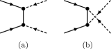
Figure 3: Two-body scattering process ${\ell}{\ell}\leftrightarrow\bar{\phi}\bar{\phi}$.

A further important washout process is ${\ell}{\ell}\leftrightarrow\bar{\phi}\bar{\phi}$ scattering which receives the $t$- and $u$-channel contributions, see Fig. 3. By analogy with Eq. (II) it is convenient to introduce

$$\Xi_{{\ell}{\ell}\leftrightarrow\bar{\phi}\bar{\phi}} \equiv{\textstyle\frac{1}{2}}\bigl{[}\Xi_{\bar{\phi}\bar{\phi}\rightarrow{\ell}{\ell}}+\Xi_{\phi\phi\rightarrow\bar{\ell}\bar{\ell}}\bigr{]}$$

$$=2(p_{1}p_{2})\textstyle\sum_{ij}M_{i}M_{j}\,\Re(h^{\dagger}h)^{2}_{ij}$$

$$\times\left[2P^{*}_{i}(t)P^{*}_{j}(t)+2P^{*}_{i}(u)P^{*}_{j}(u)\right.$$

$$+\left.P^{*}_{i}(u)P_{j}(t)+P^{*}_{i}(t)P_{j}(u)\,\right]{\,.}$$ (23)

Since the intermediate Majorana neutrino cannot go on-shell in the $t$- and $u$-channel, there is no need to use the RIS subtracted propagator in Eq. (II).

Above we have briefly reviewed the canonical approach to the computation of the lepton asymmetry, which is based on generalized Boltzmann equations. Boltzmann equations, according to conventional reasoning, describe scattering processes of particles which propagate freely over timescales large compared to the duration of individual interactions. This picture seems to be consistent with the use of $S$-matrix elements which are intended to describe transitions between asymptotically free initial and final states. However, in leptogenesis the crucial processes (CP-violating decays) involve unstable particles which spoils this picture. In vacuum the amplitudes for such processes can be computed in terms of their Feynman graphs. However the ‘naive’ way of generalizing the Boltzmann equation by multiplying the obtained amplitudes by the one-particle distributions of the initial states and integrating over phase space leads to inconsistent equations. The origin of this problem is that the obtained collision terms for particle decay and inverse decay in Eq. (7) miscount the rate of particle generation. In a short time-interval a finite number of unstable Majorana neutrinos - formed by inverse decay of particles and antiparticles - decays immediately back to either particles or antiparticles. These contributions to particle generation are not included in Eq. (7) where the amplitudes are defined in terms of Feynman graphs. For leptogenesis, in the presence of CP-violation, it leads to inconsistent equations and must be corrected. Since the missing contribution can be constructed as the rate of a two-body scattering process with on-shell intermediate state this issue can be addressed by the RIS-subtracting procedure presented above. It modifies the amplitudes for two-body scattering in order to cure the problem which appears due to the collision terms for particle decay.

III RIS subtraction with quantum statistics

It is well known that unitarity has important consequences for baryogenesis and leptogenesis Weinberg (1979); Kolb and Wolfram (1980); Roulet et al. (1998) as it implies restrictions for the CP-violating amplitudes. The issue of RIS subtraction is as well tightly related to unitarity as has been mentioned in e.g. Pilaftsis and Underwood (2004). As noted in Sec. II, the use of ‘naive’ Boltzmann equations of the kind (II) for unstable particles leads to problems such as the spurious asymmetry generation in the presence of CP-violation in the decay of the heavy neutrinos. In this section we show explicitly that the success of the RIS subtraction in thermal equilibrium is guaranteed by the unitarity of the $S$-matrix and how it can be generalized to include quantum-statistical terms. The approach to RIS subtraction differs slightly from the one discussed in the previous section.

To illustrate it we work in thermal equilibrium, ${f}_{\bar{{\ell}}}^{eq}={f}_{{\ell}}^{eq}$ and ${f}_{\bar{\phi}}^{eq}={f}_{\phi}^{eq}$, where

$${f}_{a}^{eq}=\bigl{(}e^{E_{a}/T}+\xi^{a}\bigr{)}^{-1}{\,.}$$ (24)

Subtracting from the Boltzmann equation (II) the corresponding equation for antiparticles, summing over internal degrees of freedom of the leptons and integrating with $\int\,d^{3}p/[(2\pi)^{3}E_{p}]$ we obtain in thermal equilibrium:

$$\frac{\,dn_{L}}{\,dt}=2\sum_{i}\int{\,d\Pi_{{\ell}\phi N_{i}}^{pkq}}(2\pi)^{4}\,\delta(p+k-q)$$ (25)

$$\times\bigl{[}\Xi_{N_{i}\rightarrow{\ell}\phi}-\Xi_{N_{i}\rightarrow\bar{{\ell}}\bar{\phi}}\bigr{]}(1-{f}_{{\ell}}^{eq})(1+{f}_{\phi}^{eq}){f}_{N_{i}}^{eq}$$

$$+2\int{\,d\Pi_{{\ell}\phi{\ell}\phi}^{p_{1}k_{1}p_{2}k_{2}}}(2\pi)^{4}\,\delta(p_{1}+k_{1}-p_{2}-k_{2})$$

$$\times\bigl{[}\Xi^{{}^{\prime}}_{\bar{{\ell}}\bar{\phi}\rightarrow{\ell}\phi}-\Xi^{{}^{\prime}}_{{\ell}\phi\rightarrow\bar{{\ell}}\bar{\phi}}\bigr{]}(1-{f}_{{\ell}}^{eq})(1+{f}_{\phi}^{eq}){f}_{{\ell}}^{eq}{f}_{\phi}^{eq}{\,.}$$

We can exploit the unitarity of the $S$-matrix and CPT-symmetry to obtain a requirement for a consistent approximation of the decay and scattering amplitudes. To this end we multiply Eq. (175), which follows from the generalized optical theorem at order $h^{4}$, by ${f}_{{\ell}}^{eq}{f}_{\phi}^{eq}$ and integrate over $\,d\Pi^{{\ell}}_{k}\,d\Pi^{\phi}_{p}$. Assuming Maxwell-Boltzmann equilibrium distributions we may use ${f}_{{\ell}}^{eq}{f}_{\phi}^{eq}={f}_{N_{i}}^{eq}$ in the presence of the energy conserving Dirac-delta on the right-hand-side:

$$\sum_{i}\int{\,d\Pi_{{\ell}\phi N_{i}}^{pkq}}(2\pi)^{4}\delta(p+k-q)$$

$$\hskip 42.67912pt\times\big{[}\Xi_{{N_{i}}\rightarrow{\ell}\phi}-\Xi_{{N_{i}}\rightarrow\bar{{\ell}}\bar{\phi}}\big{]}{f}_{N_{i}}^{eq}$$

$$=-\int{\,d\Pi_{{\ell}\phi{\ell}\phi}^{p_{1}k_{1}p_{2}k_{2}}}(2\pi)^{4}\delta(p_{1}+k_{1}-p_{2}-k_{2})$$

$$\hskip 42.67912pt\times\big{[}\Xi^{{}^{\prime}}_{\bar{{\ell}}\bar{\phi}\rightarrow{\ell}\phi}-\Xi^{{}^{\prime}}_{{\ell}\phi\rightarrow\bar{{\ell}}\bar{\phi}}\big{]}{f}_{{\ell}}^{eq}{f}_{\phi}^{eq}{\,.}$$ (26)

We see that imposing this as a condition for the scattering amplitudes will correctly yield $\,dn_{L}/\,dt|_{\text{eq}}=0$ if we neglect the quantum-statistical terms in (25). Equation (25) represents the zeroth-order term in an expansion about equilibrium. Using Eq. (III) we can therefore obtain consistent equations at this order without the need to specify the detailed form of $\Xi^{{}^{\prime}}_{\bar{{\ell}}\bar{\phi}\rightarrow{\ell}\phi}$ and $\Xi^{{}^{\prime}}_{{\ell}\phi\rightarrow\bar{{\ell}}\bar{\phi}}$. At higher order (for washout contributions) we also need to know the sum $\Xi^{{}^{\prime}}_{\bar{{\ell}}\bar{\phi}\rightarrow{\ell}\phi}+\Xi^{{}^{\prime}}_{{\ell}\phi\rightarrow\bar{{\ell}}\bar{\phi}}$, see Sec. IV. We know from Sec. II that relation (III) can be satisfied by subtracting RIS contributions from the tree-level two-body scattering amplitudes and taking the zero width limit:

$$\Xi^{{}^{\prime}}_{\bar{{\ell}}\bar{\phi}\rightarrow{\ell}\phi}{} =\Xi_{\bar{{\ell}}\bar{\phi}\leftrightarrow{\ell}\phi}$$

$$-{\textstyle\sum_{i}}\,\Xi_{\bar{\ell}\bar{\phi}\rightarrow{N_{i}}}\frac{\pi\delta(s-M_{i}^{2})}{2{M_{i}}0pt{i}}\Xi_{{N_{i}}\rightarrow{\ell}\phi}{\,,}$$ (27a)

$$\Xi^{{}^{\prime}}_{{\ell}\phi\rightarrow\bar{{\ell}}\bar{\phi}}{} =\Xi_{{{\ell}\phi}\leftrightarrow\bar{{\ell}}\bar{\phi}}$$

$$-{\textstyle\sum_{i}}\,\Xi_{{\ell}\phi\rightarrow{N_{i}}}\frac{\pi\delta(s-{M_{i}}^{2})}{2{M_{i}}0pt{i}}\Xi_{{N_{i}}\rightarrow\bar{{\ell}}\bar{\phi}}{\,.}$$ (27b)

Note that, strictly speaking, the RIS terms in Eq. (II) include $4(p_{1}p_{2})/M_{i}^{2}$ factors. However, upon the phase space integration in Eq. (III) the two expressions give identical results and are therefore equal in an average sense. It is obvious from comparison of Eqs. (25) and (III) that the above definition of the RIS subtracted scattering amplitudes is not sufficient to guarantee zero asymmetry in equilibrium if quantum-statistical terms are included. However this can be achieved if we replace the vacuum decay width in Eq. (27) by the thermal one Giudice et al. (2004); Kießig et al. (2010a):

$${\boldsymbol{\Gamma}}_{i}={\boldsymbol{\Gamma}}_{i}(q) \equiv\frac{1}{2g_{N}M_{i}}\int\,d\Pi^{{\ell}}_{p}\,d\Pi^{\phi}_{k}(2\pi)^{4}\delta(q-p-k)$$

$$\times\bigl{[}\Xi_{N_{i}\rightarrow{\ell}\phi}+\Xi_{N_{i}\rightarrow\bar{{\ell}}\bar{\phi}}\bigr{]}(1-{f}_{{\ell}}^{eq}+{f}_{\phi}^{eq}){\,.}$$ (28)

Using the identity $1=\int ds\int d^{4}q\delta_{+}(q^{2}-s)\delta(q-p-k)$ and the fact that the (inverse) decay amplitudes are related by CPT-symmetry we can rewrite the RIS-contribution to the second term of Eq. (25) in the form:

$$- \int ds\int\frac{d^{4}q}{(2\pi)^{3}}\delta_{+}(q^{2}-s)\sum_{i}\frac{\delta(s-M_{i}^{2})}{2M_{i}{\boldsymbol{\Gamma}}_{i}}$$

$$\times\int\,d\Pi^{{\ell}}_{p_{1}}\,d\Pi^{\phi}_{k_{1}}(2\pi)^{4}\delta(q-p_{1}-k_{1})$$

$$\hskip 62.59605pt\times{f}_{{\ell}}^{eq}{f}_{\phi}^{eq}\bigl{[}\Xi_{N_{i}\rightarrow{\ell}\phi}+\Xi_{N_{i}\rightarrow\bar{{\ell}}\bar{\phi}}\bigr{]}$$

$$\times\int\,d\Pi^{{\ell}}_{p_{2}}\,d\Pi^{\phi}_{k_{2}}(2\pi)^{4}\delta(q-p_{2}-k_{2})$$

$$\hskip 14.22636pt\times(1-{f}_{{\ell}}^{eq})(1+{f}_{\phi}^{eq})\bigl{[}\Xi_{N_{i}\rightarrow{\ell}\phi}-\Xi_{N_{i}\rightarrow\bar{{\ell}}\bar{\phi}}\bigr{]}{\,.}$$ (29)

The integration over $s$ is trivial. The $\delta_{+}(q^{2}-s)$ term ensures that after integration over $dq^{0}$ the intermediate Majorana neutrino is on-shell, $q^{2}=M_{i}^{2}$. Using ${{f}_{{\ell}}^{eq}{f}_{\phi}^{eq}}={{f}_{N_{i}}^{eq}}(1-{f}_{{\ell}}^{eq}+{f}_{\phi}^{eq})$ together with the definition (III) we can rewrite the second term of Eq. (III) as $2g_{N}M_{i}{\boldsymbol{\Gamma}}_{i}{{f}_{N_{i}}^{eq}}$ which cancels the factors coming from RIS subtraction. The resulting expression reads

$$-2 \sum_{i}\int{\,d\Pi_{{\ell}\phi N_{i}}^{pkq}}(2\pi)^{4}\,\delta(p+k-q)$$

$$\times\bigl{[}\Xi_{N_{i}\rightarrow{\ell}\phi}-\Xi_{N_{i}\rightarrow\bar{{\ell}}\bar{\phi}}\bigr{]}(1-{f}_{{\ell}}^{eq})(1+{f}_{\phi}^{eq}){f}_{N_{i}}^{eq}{\,,}$$ (30)

and cancels the first term on the right-hand side of Eq. (25). Since $\Xi_{\bar{{\ell}}\bar{\phi}\rightarrow{\ell}\phi}=\Xi_{{\ell}\phi\rightarrow\bar{{\ell}}\bar{\phi}}$ at $\mathcal{O}(h^{4})$ the new RIS subtracted source-term for the asymmetry vanishes in equilibrium.

The thermal width ${\boldsymbol{\Gamma}}_{i}$ defined in Eq. (III) would also be obtained if one computes it using thermal cutting rules instead of the optical theorem (which applies in vacuum), see Appendix B. We have seen that the unitarity of the $S$-matrix can be employed to generalize the concept of RIS subtraction to rate equations which include quantum-statistical factors. As we shall see in Sec. VII, the Majorana neutrino decay is at high temperature replaced by Higgs decay if the Higgs acquires a large effective thermal mass. In this case thermal cutting rules enforce relations between the amplitudes which can be used to obtain consistent equations, analogous to the optical theorem, see Appendix B.

Note again that in Eq. (III) we had to assume that the Majorana neutrinos are in exact thermal equilibrium. For leptogenesis this is an inconsistent assumption since the deviation of their distribution from equilibrium realizes the third Sakharov condition and drives the generation of the asymmetry. Not surprisingly, the NEQFT approach leads to a (slightly) different result for the kinetic equations. However the differences between the two approaches enter only at an order beyond the usual approximation as we will discuss in the next section.

IV Rate equations

In this section we review the derivation of rate equations, discuss in how far quantum-statistical and medium corrections can be incorporated, and compare the structure obtained when starting from the NEQFT result (2) with the conventional form. Solving a system of Boltzmann-like equations in general requires the use of numerical codes capable of treating large systems of stiff differential equations for the different momentum modes – a cumbersome task if one wants to study a wide range of model parameters. In the context of baryogenesis, a commonly employed simplification is to approximate the Boltzmann equations by the corresponding network of ‘rate equations’ for number densities $n_{a}$ or abundances $Y_{a}\equiv n_{a}/s$, where $s$ is the comoving entropy density. The resulting equations correspond to the hydrodynamical limit of the Boltzmann kinetic equations, in the comoving frame of homogeneous FRW space-time. To obtain evolution equations for ${Y_{a}}$ in the conventional approach, i.e. from Eq. (II), we therefore integrate the corresponding Boltzmann equations over $g_{a}d^{3}p/[E_{p}(2\pi)^{3}]$ to obtain, on the left-hand sides:

$$\frac{\,dn_{a}}{\,dt}+3Hn_{a}=\frac{s{\cal H}}{z}\frac{\,dY_{a}}{dz}{\,,}$$

where we have introduced the dimensionless inverse temperature $z=M_{1}/T$ and the Hubble rate ${\cal H}=H{|_{T=M_{1}}}$. In the homogeneous and isotropic Universe the derivative of the quantity $Y_{L}\equiv n_{L}/s$ can be related to the divergence of the lepton-current $j_{L}^{\mu}=(n_{L},\vec{0})$ – a quantity which is particularly easy to access in the first-principles computation – by

$${\cal D}_{\mu}j_{L}^{\mu}(t)=\frac{s{\cal H}}{z}\frac{dY_{L}}{dz}{\,.}$$

On the right-hand sides we get sums of integrated collision terms representing the effect of the different interactions. We separate contributions attributed to decays and scattering:

$$\frac{dY_{L}}{dz}=\sum_{i}\frac{dY_{L_{i}}}{dz}\bigg{|}_{D}+\frac{dY_{L}}{dz}\bigg{|}_{S}{\,.}$$ (31)

The decay contributions ${dY_{L_{i}}}/{dz}\big{|}_{D}$ to ${dY_{L}}/{dz}$ are very similar to the decay contributions ${dY_{N_{i}}}/{dz}\big{|}_{D}$ to ${dY_{N_{i}}}/{dz}$ and we can treat them in the same way. Reordering the contributions to ${dY_{L_{i}(N_{i})}}/{dz}\big{|}_{D}$ we find

$$\frac{s{\cal H}}{z} \frac{dY_{L_{i}\atop N_{i}}}{dz}\bigg{|}_{D}=\frac{s{\cal H}}{z}\frac{dY_{L_{i}\atop N_{i}}}{dz}\bigg{|}_{D,\text{extra}}$$ (32)

$$+\int{\,d\Pi_{N_{i}\phi{\ell}}^{qkp}}\bigl{[}\pm\Xi_{N_{i}\rightleftarrows{\ell}\phi}{\mathcal{F}_{{\ell}\phi\leftrightarrow N_{i}}^{pk;q}}-\Xi_{N_{i}\rightleftarrows\bar{\ell}\bar{\phi}}{\mathcal{F}_{\bar{{\ell}}\bar{\phi}\leftrightarrow N_{i}}^{pk;q}}\bigr{]}{\,,}$$

where the upper (lower) signs and arrows correspond to the rate equations for $L$ ($N_{i}$) abundance and we defined

$$\frac{s{\cal H}}{z} \frac{dY_{L_{i}}}{dz}\bigg{|}_{D,\text{extra}}\equiv\int{\,d\Pi_{N_{i}\phi{\ell}}^{qkp}}\,(2\pi)^{4}\,\delta(q-k-p)$$ (33)

$$\times\bigl{(}\Xi_{N_{i}\rightarrow{\ell}\phi}-\Xi_{{\ell}\phi\rightarrow N_{i}}\bigr{)}(1-f_{N_{i}})\bigl{[}f_{\phi}f_{{\ell}}+f_{\bar{\phi}}f_{\bar{{\ell}}}\bigr{]}{\,,}$$

which corresponds to Eq. (9), as well as

$$\frac{s{\cal H}}{z} \frac{dY_{N_{i}}}{dz}\bigg{|}_{D,\text{extra}}\equiv\int{\,d\Pi_{N_{i}\phi{\ell}}^{qkp}}\,(2\pi)^{4}\,\delta(q-k-p)$$

$$\times\bigl{(}\Xi_{{\ell}\phi\rightarrow N_{i}}-\Xi_{N_{i}\rightarrow{\ell}\phi}\bigr{)}$$

$$\times f_{N_{i}}\bigl{[}(1-f_{{\ell}})(1+f_{\phi})-(1-f_{\bar{{\ell}}})(1+f_{\bar{\phi}})\bigr{]}{\,.}$$ (34)

We used CPT-symmetry of the amplitudes in the derivation of Eqs. (33) and (IV). Later we will see that the second term in Eq. (32) appears also in the first-principle approach, compare Eq. (2), while the terms in Eqs. (33) and (IV) are absent. This motivates the separation into ‘regular’ and ‘extra’ terms performed in Eq. (32). For the contributions attributed to scattering we get:

$$\frac{s{\cal H}}{z}\frac{dY_{L}}{dz}\bigg{|}_{S} =\frac{s{\cal H}}{z}\frac{dY_{L}}{dz}\bigg{|}_{S,\text{extra}}$$ (35)

$$+\int {\,d\Pi_{{\ell}\phi{\ell}\phi}^{kpqr}}\,\textstyle\bigl{(}\Xi^{{}^{\prime}}_{\bar{{\ell}}\bar{\phi}\rightarrow{\ell}\phi}+\Xi^{{}^{\prime}}_{{\ell}\phi\rightarrow\bar{{\ell}}\bar{\phi}}\bigr{)}{\mathcal{F}_{{\ell}\phi\leftrightarrow\bar{{\ell}}\bar{\phi}}^{kp;qr}}$$

$$+\int {\,d\Pi_{{\ell}{\ell}\phi\phi}^{kpqr}}\bigl{[}\Xi_{{{\ell}}{{\ell}}\rightarrow\bar{\phi}\bar{\phi}}{\mathcal{F}_{{\ell}{\ell}\leftrightarrow\bar{\phi}\bar{\phi}}^{kp;qr}}-\Xi_{\bar{{\ell}}\bar{{\ell}}\rightarrow{\phi}{\phi}}{\mathcal{F}_{\bar{{\ell}}\bar{{\ell}}\leftrightarrow{\phi}{\phi}}^{kp;qr}}\bigr{]}{\,,}$$

with

$$\frac{s{\cal H}}{z}\frac{dY_{L}}{dz}\bigg{|}_{S,\text{extra}}=$$ (36)

$$+\int{\,d\Pi_{{\ell}\phi{\ell}\phi}^{kpqr}}\,(2\pi)^{4}\delta(k+p-q-r)\bigl{(}\Xi^{{}^{\prime}}_{\bar{{\ell}}\bar{\phi}\rightarrow{\ell}\phi}-\Xi^{{}^{\prime}}_{{\ell}\phi\rightarrow\bar{{\ell}}\bar{\phi}}\bigr{)}$$

$$\times\bigl{[}(1-f_{{\ell}})(1+f_{\phi})f_{\bar{{\ell}}}f_{\bar{\phi}}+(1-f_{\bar{{\ell}}})(1+f_{\bar{\phi}})f_{{\ell}}f_{\phi}\bigr{]}{\,,}$$

corresponding to Eq. (II). Again, Eq. (36) does not appear in the first-principle approach. Since in equilibrium the regular terms in each of Eqs. (32) and (35) vanish by detailed balance we retain Eq. (25) in the sum of decay and scattering contributions. The latter vanishes as well in equilibrium if we adopt e.g. Eq. (27) with thermal width for the RIS subtracted amplitudes $\Xi^{{}^{\prime}}_{\bar{{\ell}}\bar{\phi}\rightarrow{\ell}\phi},\,\Xi^{{}^{\prime}}_{{\ell}\phi\rightarrow\bar{{\ell}}\bar{\phi}}$. Out of equilibrium the last terms constitute a structural difference compared to the results obtained from first-principles. This difference carries over to the rate equations. We will therefore analyze these contributions separately.

The computational advantage of rate equations over full Boltzmann equations is maximized by a number of common approximations. In particular, assuming that all species are close to equilibrium and that the Majorana neutrino distribution function $f_{N_{i}}({t},{\left|{\vec{q}}\right|})$ is proportional to its equilibrium distribution for all values of the momentum $\left|\vec{q}\right|$. The temperature for all kinetic equilibrium distributions is set to a common value $T$ while finite deviations of the chemical potential with small $\mu/T$ are permitted. These approximations result for $\mu_{\ell}/T,\mu_{\phi}/T,\mu_{N_{i}}/T\ll 1$ in a closed network of rate equations for the abundances of the form (compare with Kolb and Wolfram (1980); Buchmüller et al. (2005a); Pilaftsis and Underwood (2004); Giudice et al. (2004)):

$$\frac{s{\cal H}}{z}\frac{dY_{L}}{dz}=\textstyle\sum_{i}\langle\epsilon_{i}\,\gamma^{D}_{N_{i}}\rangle\bigg{(}\frac{Y_{N_{i}}}{Y_{N_{i}}^{eq}}-1\bigg{)}$$ (37a)

$$-\frac{Y_{L}}{2\,Y_{\ell}^{eq}}(1+c_{\phi{\ell}})c_{\ell}\bigl{(}\textstyle\sum_{i}\langle\gamma^{W}_{N_{i}}\rangle+4\langle\gamma^{\prime{\ell}\phi}_{\bar{\ell}\bar{\phi}}\rangle+4\langle\gamma^{\bar{\ell}\bar{\ell}}_{\phi\phi}\rangle\bigr{)}{\,,}$$

$$\frac{s{\cal H}}{z}\frac{dY_{N_{i}}}{dz}=-\langle\gamma^{D}_{N_{i}}\rangle\bigg{(}\frac{Y_{N_{i}}}{Y_{N_{i}}^{eq}}-1\bigg{)}{\,,}$$ (37b)

where we have introduced

$$\epsilon_{i} \equiv\frac{\Xi_{N_{i}\rightarrow{\ell}\phi}-\Xi_{N_{i}\rightarrow\bar{\ell}\bar{\phi}}}{\Xi_{N_{i}}}{\,,}$$ (38a)

$$\Xi_{N_{i}} \equiv\Xi_{N_{i}\rightarrow{\ell}\phi}+\Xi_{N_{i}\rightarrow\bar{\ell}\bar{\phi}}{\,.}$$ (38b)

The factor $c_{\ell}\equiv{9\zeta(3)}/{\pi^{2}}\approx 1.1$ (we neglect the thermal lepton masses here) relates the chemical potential of the leptons to their number density,

$$\frac{\mu_{\ell}}{T}\approx c_{\ell}\cdot\frac{Y_{L}}{2Y_{{\ell}}}{\,,}$$

and the coefficient $c_{\phi{\ell}}$ takes into account that in the SM the chemical potentials of leptons and Higgs are related by $\mu_{\phi}=c_{\phi{\ell}}\cdot\mu_{\ell}$ with $c_{\phi{\ell}}=4/7$ through equilibrium gauge, Yukawa and sphaleron interactions Buchmüller et al. (2005b); Kartavtsev (2006); Harvey and Turner (1990).

Hence, the evolution of the abundances close to equilibrium is roughly governed by a few average quantities called reaction densities which describe decay and scattering processes. We will refer to $\langle\epsilon_{i}\,\gamma^{D}_{N_{i}}\rangle$, $\langle\gamma^{D}_{N_{i}}\rangle$, $\langle\gamma^{W}_{N_{i}}\rangle$ as CP-violating decay reaction density, decay reaction density and washout reaction density respectively. For comparison with standard results we want to maintain the form of Eqs. (37) and repeat their derivation from Eqs. (32) and (35) to obtain expressions for the reaction densities which take the quantum statistical factors of the Boltzmann equation into account. This is important in the present context because the thermal corrections to the CP-violating parameter, to be derived later, are of a similar kind. To this end we use that the SM gauge and Yukawa interactions keep the Higgs and leptons very close to kinetic equilibrium:

$$f_{a}=\bigl{(}e^{(E_{p}-\mu_{a})/T}+\xi^{a}\bigr{)}^{-1}{\,,}$$

with a common temperature $T_{\ell}=T_{\phi}=T$ and chemical potentials $\mu_{\ell}=-\mu_{\bar{{\ell}}}$, $\mu_{\phi}=-\mu_{\bar{\phi}}$. We shall also use ${f}_{a}^{eq}$ for the equilibrium distribution functions with zero chemical potential defined in Eq. (24).

Since a chemical potential with positive sign will appear for either the Higgs or its antiparticle, we need to include at least the thermal mass of the Higgs to be consistent. In the dense plasma gauge-, Yukawa- and Higgs self-interactions induce a large thermal Higgs mass of about $0.4\,T$. With $\mu_{\phi}/T\sim\mu_{\ell}/T\sim\epsilon_{i}^{vac}\ll m_{\phi}/T\sim 0.4$, the Higgs cannot acquire a condensate component. It is then safe to use a Bose-Einstein equilibrium distribution function to describe the distribution of the Higgs particles. Using that $(1-\xi^{a}f_{a})=\exp((E_{k}-\mu_{a})/T)f_{a}$ and hence, for a general decay collision term $N\leftrightarrow ab$ in the presence of the energy conserving Dirac-delta, $f_{a}f_{b}=\exp((\mu_{a}+\mu_{b})/{T})(1-\xi^{a}f_{a})(1-\xi^{b}f_{b})\ {f}_{N}^{eq}/(1-{f}_{N}^{eq})$, we may write:

$$\int{\,d\Pi_{Nab}^{qpk}}\Xi_{ab\leftrightarrows N}{\mathcal{F}_{ab\leftrightarrow N}^{pk;q}}=$$

$$\int{\,d\Pi_{Nab}^{qpk}}\,(2\pi)^{4}\,\delta(q-k-p)\Xi_{ab\leftrightarrows N}$$

$$\times(1-\xi^{a}f_{a})(1-\xi^{b}f_{b})\left[\frac{f_{N}-{f}_{N}^{eq}}{(1-\xi^{N}f_{N}){f}_{N}^{eq}}-(e^{\frac{\mu_{a}+\mu_{b}}{T}}-1)\right]$$

$$\times(1-\xi^{N}f_{N})\frac{{f}_{N}^{eq}}{(1-\xi^{N}{f}_{N}^{eq})}{\,.}$$ (39)

We can now expand the exponential in square brackets in the small quantity $(\mu_{a}+\mu_{b})/{T}$. If this quantity is tiny at all times the integral (IV) will not change much if we neglect quadratic and higher order terms. For the zeroth-order (first) term in square brackets we use the linear expansion $(1-\xi^{a}f_{a})(1-\xi^{b}f_{b})\approx(1-\xi^{a}{f}_{a}^{eq})(1-\xi^{b}{f}_{b}^{eq})\bigl{[}1-(\xi_{a}\frac{\mu_{a}}{T}{f}_{a}^{eq}+\xi_{b}\frac{\mu_{b}}{T}{f}_{b}^{eq})\bigr{]}$ of the prefactor. The linear order (second) term in square brackets will appear preceded by just the zeroth-order factor $(1-\xi^{a}{f}_{a}^{eq})(1-\xi^{b}{f}_{b}^{eq})=f_{ab}(1-\xi^{N}{f}_{N}^{eq})$ with

$$f_{ab}\equiv(1-\xi_{a}{f}_{a}^{eq}-\xi_{b}{f}_{b}^{eq}){\,.}$$ (40)

To write the results in a compact form we introduce decay reaction densities with quantum-statistical factors included:

$$\hskip-14.22636pt\langle X\gamma^{D}_{N_{i}}\rangle\equiv\int {\,d\Pi_{{{\ell}}{\phi}{N_{i}}}^{{p}{k}{q}}}\,(2\pi)^{4}\delta(q-k-p)X\Xi_{N_{i}}{f}_{N_{i}}^{eq}f_{{\ell}\phi},$$ (41)

and

$$\langle X\gamma^{W}_{N_{i}}\rangle\equiv\big{<}X(1-{f}_{N_{i}}^{eq})\gamma^{D}_{N_{i}}\big{>}$$ (42)

$$=\int{\,d\Pi_{{{\ell}}{\phi}{N_{i}}}^{{p}{k}{q}}}\,(2\pi)^{4}\delta(q-k-p)X\Xi_{N_{i}}(1-{f}_{N_{i}}^{eq}){f}_{N_{i}}^{eq}f_{{\ell}\phi}{\,,}$$

where $\Xi_{N_{i}}$ is the total Majorana decay amplitude. Similarly we define the scattering reaction densities as

$$\langle X\gamma^{ab}_{ij}\rangle\equiv\int {\,d\Pi_{{a}{b}{i}{j}}^{{k}{p}{q}{r}}}(2\pi)^{4}\delta(k+p-q-r)X\Xi_{ab\leftrightarrow ij}$$

$$\times (1-\xi^{a}{f}_{a}^{eq})(1-\xi^{b}{f}_{b}^{eq}){f}_{i}^{eq}{f}_{j}^{eq}{\,.}$$ (43)

Since $\Xi_{ab\leftrightarrow ij}$ refers here to a CP-symmetric (tree-level) amplitude squared we have $\langle X\gamma^{ab}_{ij}\rangle=\langle X\gamma^{ij}_{ab}\rangle$ if $X$ is symmetric as well.

With help of Eq. (C) we may separate the contributions to ${dY_{L_{i}}}/{dz}\big{|}_{D}$ into terms proportional to $\Delta f_{N_{i}}\equiv({f_{N_{i}}-{f}_{N_{i}}^{eq}})$, terms proportional to $\Delta f_{N_{i}}\cdot{\frac{\mu_{\ell}}{T}}$, or just proportional to $\mu_{\ell}/T$ (see Appendix C for details):

$$\frac{s{\cal H}}{z}\frac{dY_{L_{i}}}{dz}\Big{|}_{\Delta f_{N_{i}}}=\biggl{\langle}\epsilon_{i}\frac{\Delta f_{N_{i}}}{{f}_{N_{i}}^{eq}}\gamma^{D}_{N_{i}}\biggr{\rangle}{\,,}$$ (44a)

$$\frac{s{\cal H}}{z}\frac{dY_{L_{i}}}{dz}\Big{|}_{\Delta f_{N_{i}}{\frac{\mu_{\ell}}{T}}}=\frac{\mu_{\ell}}{T}\bigl{\langle}(c_{\phi{\ell}}{f}_{\phi}^{eq}-{f}_{{\ell}}^{eq})\frac{\Delta f_{N_{i}}}{{f}_{N_{i}}^{eq}}\gamma^{D}_{N_{i}}\bigr{\rangle}{\,,}\hphantom{aaaa}$$ (44b)

$$\frac{s{\cal H}}{z}\frac{dY_{L_{i}}}{dz}\Big{|}_{\frac{\mu_{\ell}}{T}}=-\frac{\mu_{\ell}}{T}(1+c_{\phi{\ell}})\biggl{\langle}\frac{(1-f_{N_{i}})}{(1-{f}_{N_{i}}^{eq})}\gamma^{W}_{N_{i}}\biggr{\rangle}{\,.}$$ (44c)

In addition we get with Eq. (C) for the extra term in Eq. (32):

$$\frac{s{\cal H}}{z}\frac{dY_{L_{i}}}{dz}\Big{|}_{D,\text{extra}}=2\bigl{\langle}(1-f_{N_{i}})\epsilon_{i}\gamma^{D}_{N_{i}}\bigr{\rangle}{\,.}$$ (45)

Equations (44) describe the generation of a net asymmetry due to out of equilibrium decays of heavy Majorana neutrinos. Once $\mu_{\ell}/T$ has a non-zero value, there will be a slight difference in the decay rates to particles and antiparticles respectively which is not due to CP-violation in the decay amplitude, but due to the presence of slightly different occupation numbers of leptons and Higgs in the final states of the decays. At linear order this combined effect of blocking and stimulated emission is accounted for by Eq. (44b). Depending on the ‘typical’ sign of $(c_{\phi{\ell}}{f}_{\phi}^{eq}-{f}_{{\ell}}^{eq})$ it can add to or diminish an existing asymmetry. Finally, Eq. (44c) describes washout due to inverse decays. In Sec. V we will see that the functional dependence on $f_{{\ell}\phi}=(1+{f}_{\phi}^{eq}-{f}_{{\ell}}^{eq})$ in the integrated collision terms is the same as that encountered in the CP-violating parameter $\epsilon_{i}$ itself.

Considering the last two terms in Eq. (35) we find for the scattering contributions:

$$\frac{s{\cal H}}{z}\frac{dY_{L}}{dz}\Big{|}_{S,\frac{\mu_{\ell}}{T}}=-4\frac{\mu_{\ell}}{T}(1+c_{\phi{\ell}})\big{[}\langle\gamma^{\prime{\ell}\phi}_{\bar{{\ell}}\bar{\phi}}\rangle+\langle\gamma^{{\ell}{\ell}}_{\bar{{\ell}}\bar{\phi}}\rangle\big{]}{\,,}$$ (46)

where we defined the ‘RIS subtracted reaction density’ $\langle\gamma^{\prime{\ell}\phi}_{\bar{{\ell}}\bar{\phi}}\rangle$. If we adopt the amplitudes defined in Eq. (27) in the framework of RIS subtraction, it is given by

$$\langle\gamma^{\prime{\ell}\phi}_{\bar{{\ell}}\bar{\phi}}\rangle\equiv\bigg{<}\big{[}{1-\sum_{i}\frac{\pi(1+\epsilon_{i}^{2})\Xi_{N_{i}}}{4\Xi_{{\ell}\phi\leftrightarrow\bar{{\ell}}\bar{\phi}}M_{i}0pt{i}}\delta(s-M_{i}^{2})}\big{]}\gamma^{{\ell}\phi}_{\bar{{\ell}}\bar{\phi}}\bigg{>}{\,.}$$

Note that the contribution proportional to $\epsilon_{i}^{2}$ is of higher order in $h$. Furthermore, we get for the extra term:

$$\frac{s{\cal H}}{z}\frac{dY_{L}}{dz}\Big{|}_{S,\text{extra}}\approx{}-2\sum_{i}\big{<}(1-{f}_{N_{i}}^{eq})\epsilon_{i}\gamma^{D}_{N_{i}}\big{>}$$ (47)

$$+2\frac{\mu_{\ell}}{T}\sum_{i}\big{<}\epsilon_{i}\big{(}{f}_{{\ell}}^{eq}-c_{\phi{\ell}}{f}_{\phi}^{eq}+{f}_{{\ell}}^{eq}-c_{\phi{\ell}}{f}_{\phi}^{eq}\big{)}\gamma^{W}_{N_{i}}\big{>}{\,.}$$

Here we used

$$\Big{<}\frac{(16\pi)^{2}pq\Xi_{N_{i}}\delta(s-M_{i}^{2})}{g_{w}^{2}M_{i}^{2}\Xi_{{\ell}\phi\leftrightarrow\bar{\ell}\bar{\phi}}}\gamma^{{\ell}\phi}_{\bar{{\ell}}\bar{\phi}}\Big{>}=\langle\gamma^{W}_{N_{i}}\rangle{\,.}$$ (48)

We have written Eq. (47) schematically in order to show how it compares to other washout terms. Note that the extra terms indicate that there will be a slight difference between the equations obtained in the 2PI approach and those obtained with RIS subtraction at finite temperature. Comparing Eqs. (47) and (46) we see that the first term in the former equation will cancel the latter contribution in thermal equilibrium ($f_{N_{i}}={f}_{N_{i}}^{eq}$) if the decay contributions are summed up. The second term in Eq. (47) is due to quantum statistics. Since it is proportional to $\epsilon_{i}\mu/T$ it can be large only if $\epsilon_{i}$ is large (as in the case of resonant leptogenesis). Anticipating our knowledge about the structure obtained within NEQFT, we will ignore the extra term in what follows.

At the time being, everything is still exact with respect to deviations of $f_{N_{i}}$ from equilibrium. This distribution is necessarily distorted due to the fact that it is subject to conflicting equilibrium conditions corresponding to the decay into particles and antiparticles, by the effects of the expansion and, possibly, due to non-equilibrium initial conditions. In order to obtain the full momentum-dependent distribution function we would have to solve the corresponding full kinetic equations however Basbøll and Hannestad (2007); Garayoa et al. (2009); Hahn-Woernle et al. (2009); Garny et al. (2009, 2010a).

To proceed we shall as usual assume that the deviation of the Majorana neutrinos from equilibrium is small. This allows us to neglect the ${\Delta f_{N_{i}}\frac{\mu_{\ell}}{T}}$ contribution (44b) and to replace $f_{N_{i}}\to{f}_{N_{i}}^{eq}$ in Eq. (44c). The extra terms cancel at this level of approximation up to the quantum-statistical term. In order to bring the remaining source-term Eq. (44a) into the conventional form, we need to assume that the non-equilibrium distribution of the Majorana neutrino is proportional to its equilibrium value (with momentum independent prefactor)

$$f_{N_{i}}\equiv\frac{n_{N_{i}}}{n^{eq}_{N_{i}}}{f}_{N_{i}}^{eq}{\,.}$$

With this approximation we can write

$$\biggl{\langle}X\frac{\Delta f_{N_{i}}}{{f}_{N_{i}}^{eq}}\gamma\biggr{\rangle}=\bigg{(}\frac{Y_{N_{i}}}{Y^{eq}_{N_{i}}}-1\bigg{)}\langle X\gamma\rangle{\,.}$$ (49)

The total contribution to the evolution equations for the lepton asymmetry is then given by

$$\frac{dY_{L}}{dz}=\sum_{i}\bigg{(}\frac{dY_{L_{i}}}{dz}\Big{|}_{\Delta f_{N_{i}}}+\frac{dY_{L_{i}}}{dz}\Big{|}_{\frac{\mu_{\ell}}{T}}\bigg{)}+\frac{dY_{L}}{dz}\Big{|}_{S,\frac{\mu_{\ell}}{T}}{\,,}$$ (50)

i.e. we obtain Eq. (37a). We see that, at this level of approximation, there are no contributions due to extra terms apart from those which cancel due to the RIS-subtraction. Quantitative differences can arise if the deviation of the Majorana neutrinos from equilibrium is large or $\epsilon_{i}$ is of order $1$. For the evolution of the Majorana neutrino we obtain with Appendix C, similar to Eq. (44), the decay contributions

$$\frac{s{\cal H}}{z}\frac{dY_{N_{i}}}{dz}\Big{|}_{\Delta f_{N_{i}}}=-\bigg{<}\frac{\Delta f_{N_{i}}}{{f}_{N_{i}}^{eq}}\gamma^{D}_{N_{i}}\bigg{>}{\,,}$$ (51a)

$$\frac{s{\cal H}}{z}\frac{dY_{N_{i}}}{dz}\Big{|}_{\Delta f_{N_{i}}{\frac{\mu_{\ell}}{T}}}=-\frac{\mu_{\ell}}{T}\big{<}\epsilon_{i}(c_{\phi{\ell}}{f}_{\phi}^{eq}-{f}_{{\ell}}^{eq})\frac{\Delta f_{N_{i}}}{{f}_{N_{i}}^{eq}}\gamma^{D}_{N_{i}}\big{>}{\,,}\hphantom{aaa}$$ (51b)

$$\frac{s{\cal H}}{z}\frac{dY_{N_{i}}}{dz}\Big{|}_{\frac{\mu_{\ell}}{T}}=+\frac{\mu_{\ell}}{T}(1+c_{\phi{\ell}})\bigg{<}\epsilon_{i}\frac{(1-f_{N_{i}})}{(1-{f}_{N_{i}}^{eq})}\gamma^{W}_{N_{i}}\bigg{>}{\,,}$$ (51c)

and for the extra term in Eq. (32):

$$\frac{s{\cal H}}{z}\frac{dY_{N_{i}}}{dz} \Big{|}_{D,\text{extra}}=-2\frac{\mu_{\ell}}{T}(1+c_{\phi{\ell}})\bigg{<}\epsilon_{i}\frac{(1-f_{N_{i}})}{(1-{f}_{N_{i}}^{eq})}\gamma^{W}_{N_{i}}\bigg{>}$$

$$-2\frac{\mu_{\ell}}{T}\big{<}\epsilon_{i}(c_{\phi{\ell}}{f}_{\phi}^{eq}-{f}_{{\ell}}^{eq})\frac{\Delta f_{N_{i}}}{{f}_{N_{i}}^{eq}}\gamma^{D}_{N_{i}}\big{>}{\,.}$$ (52)

Neglecting again ${\Delta f_{N_{i}}\frac{\mu_{\ell}}{T}}$ and ${\epsilon_{i}\frac{\mu_{\ell}}{T}}$ contributions we obtain

$$\frac{dY_{N_{i}}}{dz}=\frac{dY_{N_{i}}}{dz}\Big{|}_{\Delta f_{N_{i}}}{\,,}$$ (53)

i.e. Eq. (37b). If higher order contributions are taken into account, we get a difference between the conventional equations and those derived in the 2PI-formalism. Ignoring the contribution (51b) and the second term in Eq. (IV), which are due to quantum statistics, we obtain a contribution

$$\mp\frac{Y_{L}}{2\,Y_{\ell}^{eq}}\langle\epsilon_{i}\,\gamma^{W}_{N_{i}}\rangle{\,,}$$ (54)

to ${dY_{N_{i}}}/{dz}$. Here the upper sign applies if the extra terms are included and the lower sign if not. This can therefore result in the inclusion of this term with wrong sign even if quantum statistics are neglected, compare e.g. Pilaftsis and Underwood (2004).

The reaction densities for decay, $\langle\epsilon_{i}\,\gamma^{D}_{N_{i}}\rangle$, $\langle\gamma^{D}_{N_{i}}\rangle$, $\langle\gamma^{W}_{N_{i}}\rangle$, and scattering, $\langle\gamma^{\prime{\ell}\phi}_{\bar{{\ell}}\bar{\phi}}\rangle$, $\langle\gamma^{{\ell}{\ell}}_{\bar{\phi}\bar{\phi}}\rangle$, represent the hydrodynamical coefficients which govern the evolution of the number densities (abundances). We will compute them numerically once the additional medium dependence of the amplitudes (in particular the CP-violating parameters) has been derived. In addition, it is useful to define a thermally averaged CP-violating parameter as

$$\langle\epsilon_{i}\rangle\equiv\frac{\langle\epsilon_{i}\gamma^{D}_{N_{i}}\rangle}{\langle\gamma^{D}_{N_{i}}\rangle}{\,,}$$

which equals $\epsilon_{i}$ if it is momentum independent, such as in the zero temperature case, but will differ once thermal effects are included. This quantity is meaningful for the comparison with conventional results because it takes into account that the deviation of the Majorana neutrino abundance from equilibrium, which appears in the source-term for the lepton abundance, is influenced by the (CP-conserving) decay reaction density in the denominator.

Inserting conventional vacuum amplitudes in Eqs. (37) with Eqs. (41) and (42) and dropping quantum-statistical factors one obtains the conventional results for the reaction densities. For the readers convenience we quote them here. For the decay reaction density we obtain

$$\langle\gamma^{W}_{N_{i}}\rangle=\langle\gamma^{D}_{N_{i}}\rangle\approx\frac{g_{N}}{2\pi^{2}}M_{i}^{2}\Gamma_{i}TK_{1}\left(\frac{M_{i}}{T}\right){\,,}$$ (55)

and $\langle\epsilon_{i}\,\gamma^{D}_{N_{i}}\rangle=\epsilon_{i}\langle\gamma^{D}_{N_{i}}\rangle$, see Appendix A. For the two-body scattering the reaction density is given by

$$\langle\gamma^{ab}_{ij}\rangle \approx\frac{T}{64\pi^{4}}\int\limits_{s_{min}}^{\infty}ds\sqrt{s}K_{1}\left(\frac{\sqrt{s}}{T}\right)\hat{\sigma}(s){\,,}$$ (56)

where $\hat{\sigma}(s)$ is so-called reduced cross section:

$$\hat{\sigma}(s)\equiv\frac{1}{8\pi}\int\limits_{0}^{2\pi}\frac{d\varphi_{ai}}{2\pi}\int\limits_{t^{-}}^{t^{+}}\frac{dt}{s}\left|\mathcal{M}\right|_{ab\leftrightarrow ij}^{2}{\,.}$$ (57)

For the ${\ell}{\ell}\leftrightarrow\bar{\phi}\bar{\phi}$ process it reads

$$\hat{\sigma} =\frac{1}{2\pi}\sum\Re(h^{\dagger}h)^{2}_{ij}\sqrt{a_{i}a_{j}}$$ (58)

$$\times\biggl{\{}\frac{1}{a_{i}-a_{j}}\ln\left(\frac{a_{i}(x+a_{j})}{a_{j}(x+a_{i})}\right)$$

$$+\frac{1}{2}\frac{1}{x+a_{i}+a_{j}}\ln\left(\frac{(x+a_{i})(x+a_{j})}{a_{i}a_{j}}\right)\biggr{\}}{\,,}$$

where we have replaced $s$ by $x\equiv s/M_{1}^{2}$ and introduced dimensionless quantities $a_{i}\equiv M_{i}^{2}/M_{1}^{2}$ and $c_{i}\equiv\Gamma_{i}/M_{i}=(h^{\dagger}h)_{ii}/8\pi$. The case $i=j$ is included in this expression in the limiting sense $a_{j}\rightarrow a_{i}$. Note that Eq. (58) only contains the real part of $(h^{\dagger}h)^{2}$. The contribution of the imaginary part vanishes because $\Im(h^{\dagger}h)^{2}_{ij}$ is antisymmetric with respect to $i\leftrightarrow j$ whereas the sum in the curly brackets is symmetric under this transformation. The integration of Eq. (II) yields for the reduced ‘RIS subtracted cross section’ of the ${\ell}\phi\leftrightarrow\bar{\ell}\bar{\phi}$ process:

$$\hat{\sigma}^{\prime} =\frac{1}{4\pi x}\sum\Re(h^{\dagger}h)^{2}_{ij}\sqrt{a_{i}a_{j}}$$ (59)

$$\times\left\{x^{2}\frac{(x-a_{i})(x-a_{j})+(1-2\delta_{ij})a_{i}a_{j}c_{i}c_{j}}{\left[(x-a_{i})^{2}+(a_{i}c_{i})^{2}\right]\left[(x-a_{j})^{2}+(a_{j}c_{j})^{2}\right]}\right.$$

$$+2\frac{x+a_{i}}{a_{j}-a_{i}}\ln\left(\frac{x+a_{i}}{a_{i}}\right)+2\frac{x+a_{j}}{a_{i}-a_{j}}\ln\left(\frac{x+a_{j}}{a_{j}}\right)$$

$$+\frac{x-a_{i}}{(x-a_{i})^{2}+(a_{i}c_{i})^{2}}\left[x-(x+a_{j})\ln\left(\frac{x+a_{j}}{a_{j}}\right)\right]$$

$$+\left.\frac{x-a_{j}}{(x-a_{j})^{2}+(a_{j}c_{j})^{2}}\left[x-(x+a_{i})\ln\left(\frac{x+a_{i}}{a_{i}}\right)\right]\right\}{\,.}$$

The reduced ‘cross section’ (59) is negative in the vicinity of the mass shells, $x\approx a_{i}$. This is due to the $-(M_{i}\Gamma_{i})^{2}$ term in the numerator of the RIS subtracted propagator (20). Note that because we have not approximated this term by the Dirac-delta the structure of Eq. (59) is slightly different from the one usually used in the literature Pilaftsis and Underwood (2004).

V Non-equilibrium QFT approach

In this section we briefly review the description of leptogenesis within non-equilibrium quantum field theory Schwinger (1961); Keldysh (1964); Calzetta and Hu (1988); Berges (2004). This framework has been shown recently to be suitable for the derivation of quantum dynamic equations for the lepton asymmetry within a first-principle approach, and to incorporate medium, off-shell, coherence and possibly further quantum effects in a self-consistent way Buchmüller and Fredenhagen (2000); Lindner and Müller (2006); De Simone and Riotto (2007); Lindner and Müller (2008); Anisimov et al. (2009); Garny et al. (2009, 2010a); Anisimov et al. (2010a); Garny et al. (2010b); Beneke et al. (2010); Garny et al. (2010c); Beneke et al. (2011); Garbrecht (2011); Gagnon and Shaposhnikov (2011); Anisimov et al. (2010b); Drewes (2010). We continue these efforts by deriving consistent quantum corrected Boltzmann equations that describe the generation and washout of the lepton asymmetry and include the (inverse) decay as well as scattering processes mediated by Majorana neutrinos.

V.1 CTP and propagators

The lepton asymmetry is given by the $\mu=0$-component of the expectation value of the lepton-current operator:

$$j^{\mu}_{L}(x)=\bigl{\langle}{\textstyle\sum\limits_{\alpha,a}}\,\bar{\ell}^{a}_{\alpha}(x)\gamma^{\mu}{\ell}^{a}_{\alpha}(x)\bigr{\rangle}{\,.}$$

It can be expressed in terms of the leptonic two-point function. We define the two-point functions for the Higgs, lepton and Majorana fields with time arguments attached to the closed time path (CTP) shown in Fig. 4 by

$$\Delta_{ab}(x,y) =\langle T_{\cal C}\phi^{a}(x)\phi^{*b}(y)\rangle{\,,}$$ (60a)

$$S^{\alpha\beta}_{ab}(x,y) =\langle T_{\cal C}{\ell}_{\alpha}^{a}(x)\bar{\ell}_{\beta}^{b}(y)\rangle{\,,}$$ (60b)

$$\mathscr{S}^{ij}(x,y) =\langle T_{\cal C}N_{i}(x)\bar{N}_{j}(y)\rangle{\,,}$$ (60c)

where the sub- and superscripts refer to $SU(2)_{L}$ and flavor indices and $T_{\cal C}$ denotes time-ordering with respect to the CTP.

Figure 4: Closed time path.

We will frequently use matrix notation for the flavor indices, where e.g. $\hat{\mathscr{S}}$ denotes the flavor-matrix $\mathscr{S}^{ij}$, etc. Using the definition (60b) we find for the lepton-current:

$$j_{L}^{\mu}(x)=-\sum_{\alpha,a}{\rm tr}\left[\gamma_{\mu}S^{\alpha\alpha}_{aa}(x,x)\right]{\,.}$$

Two-point functions $G(x,y)$ (where $G$ stands for $\Delta$, $S$ or $\mathscr{S}$) defined on the CTP can be decomposed into a spectral function $G_{\rho}$ and statistical propagator $G_{F}$:

$$G(x,y)=G_{F}(x,y)-\frac{i}{2}\mathrm{sgn}_{\cal C}(x^{0}-y^{0})G_{\rho}(x,y){\,.}$$ (61)

The signum function is either $+1$ or $-1$ depending on whether $x^{0}$ or $y^{0}$ occur ‘later’ on the contour ${\cal C}$. $G_{F}$ and $G_{\rho}$ encode information on the state and the spectrum of the system, respectively. For example, for the leptons they are given by

$$S^{\alpha\beta}_{ab\,F}(x,y) =\frac{1}{2}\langle\left[{\ell}_{\alpha}^{a}(x),\bar{\ell}_{\beta}^{b}(y)\right]_{-}\rangle{\,,}$$

$$S^{\alpha\beta}_{ab\,\rho}(x,y) =i\langle\left[{\ell}_{\alpha}^{a}(x),\bar{\ell}_{\beta}^{b}(y)\right]_{+}\rangle{\,,}$$

where $[.,.]_{\pm}$ denote (anti-)commutators. Statistical and spectral functions of Majorana neutrino and Higgs can be expressed similarly, with $+$ and $-$ exchanged for bosons. Although there are only two independent two-point functions for each species, it is convenient to introduce additional combinations of them, namely the Wightman functions

$$G_{\gtrless}(x,y) =G_{F}(x,y)\mp\frac{i}{2}G_{\rho}(x,y){\,,}$$ (62)

as well as retarded and advanced functions,

$$G_{R}(x,y) =\Theta(x^{0}-y^{0})G_{\rho}(x,y){\,,}$$ (63a)

$$G_{A}(x,y) =-\Theta(y^{0}-x^{0})G_{\rho}(x,y){\,.}$$ (63b)

From the above definitions one can see that the difference of the retarded and advanced propagators gives the spectral one, whereas the sum yields the hermitian propagator $G_{h}(x,y)$:

$$G_{R}(x,y)-G_{A}(x,y) =G_{\rho}(x,y){\,,}$$ (64a)

$$G_{R}(x,y)+G_{A}(x,y) =2G_{h}(x,y){\,.}$$ (64b)

Finally, we will also need the CP conjugated propagators on the CTP:

$$\bar{\Delta}_{ab}(x,y) \equiv\Delta_{ba}(\bar{y},\bar{x}){\,,}$$ (65a)

$$\bar{S}^{\alpha\beta}_{ab}(x,y)\equiv (CP)S^{\beta\alpha}_{ba}(\bar{y},\bar{x})^{T}(CP)^{-1}{\,,}$$ (65b)

$$\bar{\mathscr{S}}^{ij}(x,y) \equiv(CP)\mathscr{S}^{ji}(\bar{y},\bar{x})^{T}(CP)^{-1}{\,.}$$ (65c)

Here $\bar{x}=(x^{0},-\vec{x})$, $C=i\gamma^{2}\gamma^{0}$ and $P=\gamma^{0}$ are the charge conjugation and parity matrices, respectively, and the transposition refers to spinor indices. CP conjugated statistical and spectral functions immediately follow from the above definition by inserting the decomposition (61).

V.2 Kadanoff-Baym equations for leptons

The time-evolution of the two-point functions is described self-consistently by the Kadanoff-Baym (KB) equations. These equations can be obtained from a variational principle using the so-called 2PI effective action Cornwall et al. (1974). The resulting equations of motion have the form of Schwinger-Dyson equations for the non-equilibrium propagators formulated on the CTP:

$$\hat{S}^{-1}(x,y) =\hat{S}^{-1}_{0}(x,y)-\hat{\Sigma}(x,y){\,.}$$ (66)

Here $\hat{S}^{-1}(x,y)$ is the inverse of the full lepton propagator in coordinate space, and $\hat{S}^{-1}_{0}(x,y)$ is the inverse of the free lepton propagator,

$$\hat{S}^{-1}_{0}(x,y)=\delta_{ab}\delta^{\alpha\beta}\not{\partial}_{x}\delta_{\cal C}(x-y)P_{L}{\,.}$$

The information about the interaction processes is encoded in the self-energies $\Sigma$. They can be obtained by cutting one line of the 2PI contributions to the effective actions. The two- and three-loop contributions are presented in Fig. 5.

Figure 5: Two- and three-loop contributions to the 2PI effective action and the corresponding contributions to the lepton self-energy. Note that the propagator lines used here denote full resummed propagators in contrast to those employed in the previous Feynman graphs. The contributions (a) and (c) to the 2PI effective action are known as ‘setting-sun’ and ‘mercedes’ diagrams respectively.

The KB equations can be obtained by convoluting the Schwinger-Dyson equation with the full propagator, which yields:

$$\not{\partial}_{x}S^{\alpha\beta}(x,y) =$$

$$\delta^{\alpha\beta} \delta_{\cal C}(x-y)+\int_{\cal C}d^{4}z\,\Sigma^{\alpha\gamma}(x,z)S^{\gamma\beta}(z,y){\,.}$$

Here $\int_{\cal C}d^{4}z=\int_{\cal C}dz^{0}\int d^{3}z$. After decomposing the resulting equation into statistical and spectral components, one obtains:

$$i\not{\partial}_{x}S^{\alpha\beta}_{F}(x,y) =\int_{0}^{x^{0}}\!\!d^{4}z\,\Sigma^{\alpha\gamma}_{\rho}(x,z)S^{\gamma\beta}_{F}(z,y)$$

$$-\int_{0}^{y^{0}}\!\!d^{4}z\,\Sigma^{\alpha\gamma}_{F}(x,z)S^{\gamma\beta}_{\rho}(z,y){\,,}$$ (67a)

$$i\not{\partial}_{x}S^{\alpha\beta}_{\rho}(x,y) =\int_{y^{0}}^{x^{0}}\!\!d^{4}z\,\Sigma^{\alpha\gamma}_{\rho}(x,z)S^{\gamma\beta}_{\rho}(z,y){\,.}$$ (67b)

The equations for Majorana and Higgs propagators have a similar structure, with the Klein-Gordon instead of the Dirac operator for the latter. The Schwinger-Dyson equations (66) and the corresponding Kadanoff-Baym equations (67) are formally very similar to the Schwinger-Dyson equation in vacuum. However, out of equilibrium the propagators depend not only on the relative coordinate $s=x-y$, but also on the central coordinate $X=(x+y)/2$, which makes their solution much more involved. In contrast to the Schwinger-Dyson equation in vacuum, the KB equations determine the spectral properties of the system including medium corrections, as well as the non-equilibrium dynamics of the statistical propagator self-consistently. Since the latter represents the quantum field theoretical generalization of the classical particle distribution functions, KB equations can be seen as the quantum field theoretical generalizations of Boltzmann equations.

As pointed out above, an equation of motion for the lepton asymmetry can be derived by considering the divergence of the lepton-current ${\cal D}_{\mu}j_{L}^{\mu}(x)$. Using the KB equations (67) one obtains:

$${\cal D}_{\mu}j_{L}^{\mu}(x) =-g_{w}\lim_{y\rightarrow x}({\cal D}_{x}^{\mu}+{\cal D}_{y}^{\mu}){\rm tr}\left[\gamma_{\mu}S^{\alpha\alpha}(x,y)\right]$$

$$=g_{w}\,i\int_{0}^{x^{0}}\mathscr{D}^{4}z\,{\rm tr}\bigl{[}\Sigma^{\alpha\beta}_{\rho}(x,z)S^{\beta\alpha}_{F}(z,x)$$

$$-\Sigma^{\alpha\beta}_{F}(x,z)S^{\beta\alpha}_{\rho}(z,x)-S^{\alpha\beta}_{\rho}(x,z)\Sigma^{\beta\alpha}_{F}(z,x)$$

$$+S^{\alpha\beta}_{F}(x,z)\Sigma^{\beta\alpha}_{\rho}(z,x)\bigr{]}{\,.}$$ (68)

Here summation over repeated indices is implicitly assumed. The two equations above represent the quantum generalization of the Boltzmann equation for the lepton asymmetry. Thus, they may be considered as the master equations for a quantum field theoretical treatment of leptogenesis Buchmüller and Fredenhagen (2000); De Simone and Riotto (2007).

The dependence of the two-point functions on the relative coordinate $s$ is characterized by the hard scales like the Majorana neutrino mass $M_{1}$ or the temperature $T$ of the surrounding plasma. In contrast to that, the variation with the central coordinate $X$ is given by the macroscopic time-evolution of the system, e.g. the Hubble rate $H$ or the Majorana decay rate $\Gamma$. Therefore, it is possible to perform an expansion in slow relative to fast time-scales, i.e. in powers of e.g. $\Gamma/M_{1}$ or $H/T$. Technically, this can be realized by a so-called gradient or derivative expansion with respect to $X$, and a Fourier transformation with respect to $s$, known as Wigner transformation, see Appendix D for more details. Then, to leading order in the gradients, the evolution equation (V.2) for the lepton asymmetry becomes Markovian, and after some straightforward algebra, can be written as

$${\cal D}_{\mu}j^{\mu}_{\ell}(t) =g_{w}\int\limits_{0}^{\infty}\frac{dp^{0}}{2\pi}\int\frac{d^{3}p}{(2\pi)^{3}}$$ (69)

$$\times{\rm tr}\bigl{\{}\bigl{[}\Sigma^{\alpha\beta}_{<}(t,p)S^{\beta\alpha}_{>}(t,p)-\Sigma^{\alpha\beta}_{>}(t,p)S^{\beta\alpha}_{<}(t,p)\bigr{]}$$

$$-\bigl{[}\bar{\Sigma}^{\beta\alpha}_{<}(t,p)\bar{S}^{\alpha\beta}_{>}(t,p)-\bar{\Sigma}^{\beta\alpha}_{>}(t,p)\bar{S}^{\alpha\beta}_{<}(t,p)\bigr{]}\bigr{\}}{\,.}$$

Note that it is possible to investigate higher orders in the derivative expansion systematically Garny et al. (2010c). In Eq. (69) all two-point functions are evaluated in Wigner space, where $p$ is the physical momentum Hohenegger et al. (2008) that corresponds to $s$. For a spatially homogeneous system (like FRW) the two-point functions depend only on the time coordinate $t=X^{0}$, and on the momentum $p$, because of spatial translational invariance. Strictly speaking, this is true only in the rest frame of the medium (comoving frame). In a general frame the two-point functions depend on $X\cdot u$, where $u_{\mu}$ is the four-velocity of the medium. The latter satisfies the normalization condition $u^{\mu}u_{\mu}=1$, and is given by $u=(1,0,0,0)$ in the medium rest frame.

In order to allow for a physical interpretation of Eq. (69) we have written it such that the integration is over positive frequencies only, and expressed the lepton propagator and self-energy in terms of the Wigner transformed Wightman functions Eq. (62). In thermal equilibrium, the Wightman functions depend only on the momentum $p$ and satisfy the Kubo-Martin-Schwinger (KMS) relation $G_{>}^{th}(p)=\pm e^{p\cdot u/T}G_{<}^{th}(p)$ for fermions/bosons, respectively. When inserting the KMS relations for propagators and self-energies into Eq. (69), one immediately finds that the divergence of the lepton-current vanishes in thermal equilibrium as it should (see also Beneke et al. (2010)). In other words, the quantum equation for the lepton asymmetry is in accordance with the third Sakharov condition. We emphasize that it is not necessary to apply RIS subtraction to obtain this result within the CTP approach Garny et al. (2009, 2010a); Beneke et al. (2010).

The four terms on the right-hand side of Eq. (69) may be interpreted as gain and loss terms of leptons and anti-leptons respectively Garny et al. (2009, 2010a). In particular, one may define generalized lepton distribution functions $f_{\ell}^{\alpha\beta}(t,p)$ via the so-called Kadanoff-Baym ansatz

$$S^{\alpha\beta}_{>}=(1-f_{\ell}^{\alpha\beta})S^{\alpha\beta}_{\rho}{\,,}\quad S^{\alpha\beta}_{<}=-f_{\ell}^{\alpha\beta}S^{\alpha\beta}_{\rho}{\,.}$$ (70)

Thus the contribution on the right-hand side of Eq. (69) that contains $S^{\beta\alpha}_{<}$ corresponds to the lepton loss term, while the contribution proportional to $S^{\beta\alpha}_{>}$ represents the lepton gain term. Analogous definitions relate the CP conjugate propagators with the anti-lepton distribution. Note that the KMS relations ensure that in equilibrium $f$ approaches the Fermi-Dirac distribution $f_{\ell}^{\alpha\beta}\to\delta^{\alpha\beta}{f}_{FD}^{eq}$. The flavor off-diagonal components encode coherent flavor correlations Beneke et al. (2011). In the unflavored regime considered here $f_{\ell}^{\alpha\beta}=\delta^{\alpha\beta}f_{\ell}$ and $S^{\alpha\beta}=\delta^{\alpha\beta}S$. In the quasiparticle (QP) approximation, the spectral function is given by

$$S^{\alpha\beta}_{\rho}(t,p) =(2\pi)\,\mathrm{sign}(p^{0})\,\delta(p^{2}-m_{\ell}^{2})\,\delta^{\alpha\beta}\,P_{L}\not{p}P_{R}$$

$$\equiv\mathbf{S}_{\rho}\,\delta^{\alpha\beta}\,P_{L}\not{p}P_{R}{\,,}$$ (71)

where we assume that leptons obey conventional dispersion relation and $m_{\ell}$ is the effective thermal mass. These assumptions might be modified in the presence of a medium Weldon (1989); Giudice et al. (2004); Kießig et al. (2010b).

Due to the presence of the Dirac-delta-function in Eq. (V.2) the integration over $p^{0}$ in Eq. (69) is trivial and leaves only the integration over spatial momenta of on-shell leptons. Therefore the right-hand side of Eq. (69) can be interpreted as a difference of two (integrated) Boltzmann-like equations – one for the particles and one for the antiparticles Garny et al. (2010a). According to the physical interpretation of Eq. (69) in terms of gain and loss terms, the Wightman components of the lepton self-energy and of its CP conjugate are the analogs of the collision integrals. Since we limit our analysis to the unflavored regime, it is convenient to perform the summation over the flavor indices: $\delta^{\alpha\beta}\Sigma^{\alpha\beta}=\Sigma^{\alpha\alpha}\equiv\Sigma$. Then the one-loop contribution, see Fig. 5 (b), takes the form:

$$\Sigma^{(1)}_{\gtrless}(t,p)= -\int\,d\Pi^{4}_{k}\,d\Pi^{4}_{q}(2\pi)^{4}\delta(p+k-q)$$

$$\times(h^{\dagger}h)_{ji}\,P_{R}\mathscr{S}^{ij}_{\gtrless}(t,q)P_{L}\Delta_{\lessgtr}(t,k){\,,}$$ (72)

where $\,d\Pi^{4}_{q}\equiv{d^{4}q}/{(2\pi)^{4}}$. The explicit expression for the two-loop contribution is rather lengthy and it is convenient to split it into three distinct terms:

$$\Sigma^{(2)}_{\gtrless}=\Sigma^{(2.1)}_{\gtrless}+\Sigma^{(2.2)}_{\gtrless}+\Sigma^{(2.3)}_{\gtrless}{\,.}$$ (73)

The first term on the right-hand side reads

$$\Sigma^{(2.1)}_{\gtrless}(t,p)=\int\,d\Pi^{4}_{q}\,d\Pi^{4}_{k}\ (2\pi)^{4}\delta(p+k-q)$$ (74)

$$\times\big{[}(h^{\dagger}h)_{in}(h^{\dagger}h)_{jm}\varLambda_{mn}(t,q,k)P_{L}C\mathscr{S}^{ij}_{\gtrless}(t,q)P_{L}\Delta_{\lessgtr}(t,k)$$

$$+(h^{\dagger}h)_{ni}(h^{\dagger}h)_{mj}P_{R}\mathscr{S}^{ji}_{\gtrless}(t,q)CP_{R}V_{nm}(t,q,p)\Delta_{\lessgtr}(t,k)\big{]}{\,,}$$

where we have introduced two functions containing loop corrections:

$$\varLambda_{mn}(t,q,k)\equiv\int\,d\Pi^{4}_{k_{1}}\,d\Pi^{4}_{k_{2}}\,d\Pi^{4}_{k_{3}}$$

$$\times(2\pi)^{4}\delta(q+k_{1}+k_{2})\ (2\pi)^{4}\delta(k+k_{2}-k_{3})$$

$$\times\bigl{[}P_{R}\mathscr{S}^{mn}_{R}(t,-k_{3})CP_{R}S^{T}_{F}(t,k_{2})\Delta_{A}(t,k_{1})$$

$$+\ P_{R}\mathscr{S}^{mn}_{F}(t,-k_{3})CP_{R}S^{T}_{R}(t,k_{2})\Delta_{A}(t,k_{1})$$

$$+\ P_{R}\mathscr{S}^{mn}_{R}(t,-k_{3})CP_{R}S^{T}_{A}(t,k_{2})\Delta_{F}(t,k_{1})\bigr{]}{\,,}$$ (75)

and $V_{nm}(t,q,k)\equiv P\,\varLambda^{\dagger}_{nm}(t,q,k)\,P$ to shorten the notation. Comparing Eqs. (V.2) and (74) we see that they have a very similar structure. First, the integration is over momenta of the Higgs and Majorana neutrino and the delta-function contains the same combination of the momenta. Second, both self-energies include one Wightman propagator of the Higgs field and one Wightman propagator of the Majorana field. Upon the use of the Kadanoff-Baym ansatz the Wightman propagators can be interpreted as cut-propagators which describe on-shell particles created from or absorbed by the plasma Carrington and Mrowczynski (2005). On the other hand, the retarded and advanced propagators can be associated with the off-shell intermediate states. We therefore conclude that Eqs. (V.2) and (74) describe (inverse) decays of the heavy neutrino into a lepton-Higgs pair.

The second term on the right-hand side of Eq. (73) contains two Wightman propagators of the Higgs field and one Wightman propagator of the lepton field. The Majorana propagator appears only in the intermediate state:

$$\Sigma^{(2.2)}_{\gtrless}(t,p)=\int\,d\Pi^{4}_{p_{2}}\,d\Pi^{4}_{k_{1}}\,d\Pi^{4}_{k_{2}}(2\pi)^{4}\delta(p+k_{1}-p_{2}-k_{2})$$

$$\times(h^{\dagger}h)_{ni}(h^{\dagger}h)_{mj}\bigl{[}P_{R}\mathscr{S}^{ij}_{R}(t,p_{2}+k_{2})CP_{R}S^{T}_{\lessgtr}(t,-p_{2})P_{L}$$

$$\times C\mathscr{S}^{mn}_{A}(t,p_{2}-k_{1})P_{L}\Delta_{\lessgtr}(t,k_{1})\Delta_{\lessgtr}(t,-k_{2})\bigr{]}{\,.}$$ (76)

We therefore conclude that this term describes lepton number violating scattering processes mediated by the heavy neutrino. Finally the last term in Eq. (73) contains two Wightman propagators of the Majorana field and one of the lepton field, whereas the Higgs field is in the intermediate state:

$$\Sigma^{(2.3)}_{\gtrless}(t,p)=\int d\Pi_{p_{2}}d\Pi_{k_{1}}d\Pi_{k_{2}}(2\pi)^{4}\delta(p+q_{1}-p_{2}-q_{2})$$

$$\times(h^{\dagger}h)_{ij}(h^{\dagger}h)_{lk}\bigl{[}P_{R}\mathscr{S}^{jk}_{\gtrless}(t,-q_{1})CP_{R}S^{T}_{\gtrless}(t,p_{2})P_{L}C$$

$$\times\mathscr{S}^{li}_{\gtrless}(t,q_{2})P_{L}\Delta_{A}(t,-q_{2}-p_{2})\Delta_{R}(t,q_{1}-p_{2})\bigr{]}{\,.}$$ (77)

Therefore it can be identified with the Higgs mediated scattering processes. These conserve lepton number and do not contribute to generation of the lepton asymmetry.

The CP conjugate of the Wigner transforms can be obtained using Eq. (65). In practice this amounts to replacing the propagators by their CP conjugate and the couplings by their complex conjugate in the above expressions. For instance for the CP conjugate of the one-loop self-energy we find:

$$\bar{\Sigma}^{(1)}_{\gtrless}(t,p)= -\int\,d\Pi^{4}_{k}\,d\Pi^{4}_{q}(2\pi)^{4}\delta(k+p-q)$$

$$\times(h^{\dagger}h)^{*}_{ji}\,P_{R}\bar{\mathscr{S}}^{ij}_{\gtrless}(t,q)P_{L}\bar{\Delta}_{\lessgtr}(t,k){\,.}$$ (78)

Expression for the CP conjugate of the two-loop lepton self-energy can be obtained in a similar way.

For the Higgs propagators in the above self-energies we can also use the Kadanoff-Baym ansatz,

$$\Delta_{>}=(1+f_{\phi})\Delta_{\rho}{\,,}\quad\Delta_{<}=f_{\phi}\Delta_{\rho}{\,,}$$ (79)

and the simple quasiparticle approximation for the spectral function,

$$\Delta_{\rho}(t,k)=\,(2\pi)\,\mathrm{sign}(k^{0})\,\delta(k^{2}-m_{\phi}^{2}){\,,}$$ (80)

where $m_{\phi}$ is the effective thermal mass. Effects of the finite thermal Higgs mass will be studied in Sec. VII.

VI Majorana contribution

In this section we will analyze the lepton number and CP-violating (inverse) decay of the Majorana neutrino as well as the two-body scattering processes mediated by the heavy neutrino. In particular, we will derive expressions for the in-medium CP-violating parameters, decay widths and scattering amplitudes. We will also explicitly demonstrate that the obtained equation for the lepton asymmetry is free of the double-counting problem.

VI.1 Decay at tree-level approximation

In the previous section we have used the Kadanoff-Baym ansatz and quasiparticle approximation for the Higgs and lepton fields. Let us now assume that similar approximations also hold for Majorana neutrinos. That is, we assume that in Eqs. (V.2) and (V.2) the spectral function $\mathscr{S}^{ij}_{\rho}$ is diagonal in flavor space and can be approximated by

$$\mathscr{S}^{ij}_{\rho} =(2\pi)\,\mathrm{sign}(q^{0})\delta(q^{2}-M_{i}^{2})\,\delta_{ij}\,(\not{q}+M_{i}){\,,}$$ (81)

and that it is related to the Wightmann components via the Kadanoff-Baym ansatz:

$$\mathscr{S}^{ii}_{>}=(1-f_{N_{i}})\mathscr{S}^{ii}_{\rho},\quad\mathscr{S}^{ii}_{<}=-f_{N_{i}}\mathscr{S}^{ii}_{\rho}{\,.}$$ (82)

Substituting Eqs. (V.2) and (V.2) in Eq. (69) and making the above approximations we find after some algebra that the lepton-current can be represented in the form:

$${\cal D}_{\mu}j_{L}^{\mu}(t) =\sum_{i}\int{\,d\Pi_{N_{i}{\ell}\phi}^{qpk}}$$

$$\times\bigl{[}\Xi_{{\ell}\phi\leftrightarrow N_{i}}{\mathcal{F}_{{\ell}\phi\leftrightarrow N_{i}}^{pk;q}}-\Xi_{\bar{\ell}\bar{\phi}\leftrightarrow N_{i}}{\mathcal{F}_{\bar{\ell}\bar{\phi}\leftrightarrow N_{i}}^{pk;q}}\bigr{]}{\,,}$$ (83)

where $\cal F$ have been introduced in Eq. (I) and we have defined:

$$\Xi^{T}_{{\ell}\phi\leftrightarrow N_{i}} \equiv g_{w}(h^{\dagger}h)_{ii}{\rm tr}[(\not{q}+M_{i})P_{L}\not{p}\,]{\,,}$$ (84a)

$$\Xi^{T}_{\bar{\ell}\bar{\phi}\leftrightarrow N_{i}} \equiv g_{w}(h^{\dagger}h)_{ii}{\rm tr}[(\not{q}+M_{i})P_{L}\not{p}\,]{\,.}$$ (84b)

The superscript ‘T’ stands for ‘tree-level’. The expression (VI.1) strongly resembles the Boltzmann equation. Therefore the functions $\Xi^{T}_{{\ell}\phi\leftrightarrow N_{i}}$ and $\Xi^{T}_{\bar{\ell}\bar{\phi}\leftrightarrow N_{i}}$ can be interpreted as effective in-medium amplitudes squared, summed over internal degrees of freedom, for the decays into leptons and antileptons respectively.

Figure 6: Tree-level contribution.

The two effective amplitudes (84) can be replaced by the total decay amplitude and the CP-violating parameter. Using Eq. (84) we find that within the used approximations the resulting decay amplitude coincides with the outcome of the vacuum calculation, $\Xi_{N_{i}}=4g_{w}(h^{\dagger}h)_{ii}(pq)$, and that $\epsilon_{i}=0$.

In the presence of a nonzero lepton asymmetry $f_{\ell}\neq f_{\bar{\ell}}$ and $f_{\phi}\neq f_{\bar{\phi}}$. Therefore ${\mathcal{F}_{{\ell}\phi\leftrightarrow N_{i}}^{pk;q}}\neq{\mathcal{F}_{\bar{\ell}\bar{\phi}\leftrightarrow N_{i}}^{pk;q}}$ and this leads to a washout of the asymmetry. Despite the fact that Eq. (VI.1) correctly describes the (leading-order) washout processes, it fails to describe processes which generate lepton asymmetry: in the considered approximation $\epsilon_{i}=0$ because the CP-violating effects, which are required to produce the asymmetry, are of fourth order in the Yukawa couplings of the Majorana neutrino. In Eq. (84) we have taken into account only terms quadratic in the coupling. In other words, this approximation corresponds to the tree-level approximation in the canonical approach.

Terms of higher order in the couplings emerge from three- and higher-loop contributions to the lepton self-energy, see Eqs. (73)-(V.2), as well as from expansion of the full Majorana propagators entering the self-energies.

VI.2 Equilibrium solution for Majorana propagator

In order to define an effective CP-violating parameter and decay width that incorporate medium corrections we have to identify the quasiparticle excitations in the system. To perform this analysis we follow the discussion of the self-energy contribution within a toy-model as presented in Garny et al. (2010a). As has been demonstrated there, it is important to take the matrix structure of the Majorana propagator in flavor space into account. Our starting point is the Schwinger-Dyson equation for the Majorana two-point function:

$$\hat{\mathscr{S}}^{-1}(x,y) =\hat{\mathscr{S}}^{-1}_{0}(x,y)-\hat{\Pi}(x,y){\,.}$$ (85)

Let us split the self-energy into diagonal and off-diagonal components in flavor space and introduce a diagonal propagator $\mathcal{S}$ defined by the equation:

$$\hat{\mathcal{S}}^{-1}(x,y)=\hat{\mathcal{S}}^{-1}_{0}(x,y)-\hat{\Pi}^{d}(x,y){\,,}$$ (86)

where $\hat{\mathcal{S}}_{0}$ is the free propagator and $\hat{\Pi}^{d}$ denotes the diagonal components of the self-energy. The poles of the diagonal propagator define the quasiparticle excitations. It can be shown that the dynamics of these is described by a Boltzmann-like quantum kinetic equation.

Inserting this decomposition into the Schwinger-Dyson equation we find, using matrix notation:

$$\hat{\mathscr{S}}^{-1}(x,y)=\hat{\mathcal{S}}^{-1}(x,y)-\hat{\Pi}^{{}^{\prime}}(x,y){\,,}$$ (87)

where $\hat{\Pi}^{{}^{\prime}}$ denotes the off-diagonal components of the self-energy and $\hat{\mathscr{S}}$ the full neutrino propagator including flavor-diagonal and flavor off-diagonal contributions. Multiplying Eq. (87) by $\hat{\mathscr{S}}$ from the left, by $\hat{\mathcal{S}}$ from the right and integrating over the contour $\cal C$ we obtain a formal solution for the full non-equilibrium propagator:

$$\hat{\mathscr{S}}(x,y) =\hat{\mathcal{S}}(x,y)$$

$$+\int_{\mathcal{C}}\mathscr{D}^{4}u\mathscr{D}^{4}v\hat{\mathscr{S}}(x,u)\hat{\Pi}^{{}^{\prime}}(u,v)\hat{\mathcal{S}}(v,y){\,.}$$ (88)

After decomposing the propagators and self-energies into the spectral and statistical components, we can rewrite Eq. (VI.2) in the form:

$$\hat{\mathscr{S}}_{F(\rho)}(x,y) =\hat{\mathcal{S}}_{F(\rho)}(x,y)-\int\mathscr{D}^{4}u\mathscr{D}^{4}v\theta(u^{0})\theta(v^{0})$$

$$\times\bigl{[}\hat{\mathscr{S}}_{R}(x,u)\hat{\Pi}^{{}^{\prime}}_{R}(u,v)\hat{\mathcal{S}}_{F(\rho)}(v,y)$$

$$+\hat{\mathscr{S}}_{R}(x,u)\hat{\Pi}^{{}^{\prime}}_{F(\rho)}(u,v)\hat{\mathcal{S}}_{A}(v,y)$$

$$+\hat{\mathscr{S}}_{F(\rho)}(x,u)\hat{\Pi}^{{}^{\prime}}_{A}(u,v)\hat{\mathcal{S}}_{A}(v,y)\bigr{]}{\,.}$$ (89)

Here we are using the retarded and advanced propagators defined by Eq. (63), so that the integration can be extended to the whole $uv$-plane. Using their definitions and Eq. (VI.2), we can also derive formal solutions for the retarded and advanced propagators:

$$\hat{\mathscr{S}}_{R(A)}(x,y) =\hat{\mathcal{S}}_{R(A)}(x,y)-\int\mathscr{D}^{4}u\mathscr{D}^{4}v\theta(u^{0})\theta(v^{0})$$

$$\times \hat{\mathscr{S}}_{R(A)}(x,u)\hat{\Pi}^{{}^{\prime}}_{R(A)}(u,v)\hat{\mathcal{S}}_{R(A)}(v,y){\,.}$$ (90)

Next we Wigner transform Eqs. (VI.2) and (VI.2) and perform the leading order gradient expansion as has been outlined in Sec. V. Combining both results, we find for the full statistical and spectral propagators and the corresponding causal two-point functions of the system in to equilibrium:

$$\hat{\mathscr{S}}_{F(\rho)} =\hat{\mathcal{S}}_{F(\rho)}-\hat{\mathscr{S}}_{R}\hat{\Pi}^{{}^{\prime}}_{R}\hat{\mathcal{S}}_{F(\rho)}$$

$$-\hat{\mathscr{S}}_{R}\hat{\Pi}^{{}^{\prime}}_{F(\rho)}\hat{\mathcal{S}}_{A}-\hat{\mathscr{S}}_{F(\rho)}\hat{\Pi}^{{}^{\prime}}_{A}\hat{\mathcal{S}}_{A},$$ (91a)

$$\hat{\mathscr{S}}_{R(A)} =\hat{\mathcal{S}}_{R(A)}-\hat{\mathscr{S}}_{R(A)}\hat{\Pi}^{{}^{\prime}}_{R(A)}\hat{\mathcal{S}}_{R(A)}{\,,}$$ (91b)

where all propagators and self-energies are evaluated at the same point $(X,q)$ in configuration space. We can express the full statistical and spectral propagators in terms of the diagonal ones and the off-diagonal self-energies,

$$\hat{\mathscr{S}}_{F(\rho)}=\hat{\Theta}_{R}\bigl{[}\hat{\mathcal{S}}_{F(\rho)}-\hat{\mathcal{S}}_{R}\hat{\Pi}^{{}^{\prime}}_{F(\rho)}\hat{\mathcal{S}}_{A}\bigr{]}\hat{\Theta}_{A}{\,,}$$ (92)

where $\hat{\Theta}_{R}$ and $\hat{\Theta}_{A}$ are defined by $\hat{\Theta}_{R}\equiv\bigl{(}\textbf{I}+\hat{\mathcal{S}}_{R}\hat{\Pi}^{{}^{\prime}}_{R}\bigr{)}^{-1}$ and $\hat{\Theta}_{A}\equiv\bigl{(}\textbf{I}+\hat{\Pi}^{{}^{\prime}}_{A}\hat{\mathcal{S}}_{A}\bigr{)}^{-1}$ respectively, with I being the $4n\times 4n$ unit matrix in the Dirac and flavor space of the $n$ generations. Solution Eq. (92) reduces the dynamics of the full statistical and spectral propagators to the dynamics of two quasiparticle excitations. Their masses, decay widths and CP-violating parameters are determined by the medium and the abundances are described by the corresponding one-particle distribution functions. Strictly speaking, the solution (92) is valid only in thermal equilibrium. However, we assume that it also holds for small deviations from equilibrium.

To consistently analyze processes of the fourth order in the coupling one has to use so-called extended quasiparticle approximation (eQP) for the statistical propagator and spectral function Spicka and Lipavsky (1994, 1995); Morozov and Röpke (2006a); Köhler and Malfliet (1993); Morozov and Röpke (2006b). The eQP approximation represents the diagonal propagator as a sum of two terms:

$$\hat{\mathcal{S}}_{\gtrless} =\hat{\tilde{\mathcal{S}}}_{\gtrless}-{\textstyle\frac{1}{2}}\bigl{(}\hat{\mathcal{S}}_{R}\hat{\Pi}^{d}_{\gtrless}\hat{\mathcal{S}}_{R}+\hat{\mathcal{S}}_{A}\hat{\Pi}^{d}_{\gtrless}\hat{\mathcal{S}}_{A}\bigr{)}{\,.}$$ (93)

The first describes decay processes, whereas the second can be associated with scattering processes. Inserting Eq. (93) into Eq. (92) we get a solution for the resummed Majorana propagator consistent up to the fourth order in the couplings:

$$\hat{\mathscr{S}}_{\gtrless} =\hat{\Theta}_{R}\bigl{[}\,\hat{\tilde{\mathcal{S}}}_{\gtrless}$$

$$-\hat{\mathcal{S}}_{R}\hat{\Pi}^{{}^{\prime}}_{\gtrless}\hat{\mathcal{S}}_{A}-{\textstyle\frac{1}{2}}\bigl{(}\hat{\mathcal{S}}_{R}\hat{\Pi}^{d}_{\gtrless}\hat{\mathcal{S}}_{R}+\hat{\mathcal{S}}_{A}\hat{\Pi}^{d}_{\gtrless}\hat{\mathcal{S}}_{A}\bigr{)}\bigr{]}\hat{\Theta}_{A}{\,.}$$ (94)

The first term in the above formula describes Majorana decay, see Sec. VI.3, whereas the remaining three terms describe the two-body scattering processes mediated by the Majorana neutrino. These are discussed in Sec. VI.4.

Using definition of the retarded and advanced two-point functions, Eq. (63), and the Schwinger-Dyson equation for the diagonal propagators, Eq. (86), we find that the causal propagators in Eq. (VI.2) are given by

$$\hat{\mathcal{S}}_{R(A)}=-\bigl{(}\not{q}-\hat{M}-\hat{\Pi}_{R(A)}\bigr{)}^{-1}{\,.}$$ (95)

Splitting the retarded and advanced self-energies into the vector and scalar components we can write the solution of Eq. (95) in the form:

$$\mathcal{S}_{R(A)} =-\frac{\bigl{(}\not{q}-\not{\Pi}^{v}_{R(A)}\bigr{)}+\bigl{(}M+\Pi^{s}_{R(A)}\bigr{)}}{\bigl{(}q-\Pi^{v}_{R(A)}\bigr{)}^{2}-\bigl{(}M+\Pi^{s}_{R(A)}\bigr{)}^{2}}$$

$$\equiv-\frac{\Omega_{h}\mp\frac{i}{2}\not{\Pi}^{v}_{\rho}}{{\boldsymbol{\Omega}}_{h}\pm i{\boldsymbol{\Pi}}_{\rho}}{\,,}$$ (96)

where we have omitted flavor indices to shorten the notation and introduced

$$\Omega_{h} \equiv\bigl{(}\not{q}-\not{\Pi}^{v}_{h}\bigr{)}+\bigl{(}M+\Pi^{s}_{h}\bigr{)}{\,,}$$

$${\boldsymbol{\Omega}}_{h} \equiv\bigl{(}q-\Pi^{v}_{h}\bigr{)}^{2}-\bigl{(}M+\Pi^{s}_{h}\bigr{)}^{2}-\bigl{(}{\textstyle\frac{1}{2}}\Pi^{v}_{\rho}\bigr{)}^{2}{\,,}$$

$${\boldsymbol{\Pi}}_{\rho} \equiv\Pi^{v}_{h}\Pi^{v}_{\rho}-q\Pi^{v}_{\rho}{\,.}$$

From Eq. (VI.2) we can extract the spectral and hermitian propagators. To leading order in the Yukawas they read

$$\mathcal{S}_{\rho}\approx+\Omega_{h}\,\frac{2\,{\boldsymbol{\Pi}}_{\rho}}{{\boldsymbol{\Omega}}^{2}_{h}+{\boldsymbol{\Pi}}^{2}_{\rho}}\equiv\Omega_{h}\boldsymbol{\mathcal{S}}_{\rho}{\,,}$$ (97a)

$$\mathcal{S}_{h}\approx-\Omega_{h}\,\frac{{\boldsymbol{\Omega}}_{h}}{{\boldsymbol{\Omega}}^{2}_{h}+{\boldsymbol{\Pi}}^{2}_{\rho}}\equiv\Omega_{h}\boldsymbol{\mathcal{S}}_{h}{\,.}$$ (97b)

The on-shell condition is defined by ${\boldsymbol{\Omega}}_{h}=0$. Expanding ${\boldsymbol{\Omega}}_{h}$ to linear order in the Yukawas we find:

$${\boldsymbol{\Omega}}_{h} \approx\bigl{(}q^{2}-M^{2}\bigr{)}\left(1-2\Gamma/\pi M\right)$$

$$+(\Gamma/\pi M)\,q^{2}\ln\left(|q^{2}|/M^{2}\right)-2q\Pi^{v,med}_{h}{\,,}$$

where $\not{\Pi}^{v,med}_{h}$ is the medium-induced component of the hermitian self-energy in the on-shell renormalization scheme. In vacuum the on-shell condition is fulfilled for $q^{2}=M^{2}$, i.e. $M$ is the physical vacuum mass. At non-zero temperatures the mass receives medium-induced corrections. To linear order in the Yukawas the effective mass is given by ${\boldsymbol{M}}^{2}\approx M^{2}+2q\Pi^{v,med}_{h}$. For a hierarchical mass spectrum, which we consider here, the contributions of the hermitian self-energy are always negligible and we will use ${\boldsymbol{\Omega}}_{h}\approx q^{2}-M^{2}$ and $\Omega_{h}\approx\not{q}-M$ in the following. From Eq. (97) we can also deduce the effective width. To leading order in the Yukawas it is given by ${\boldsymbol{M}}{\boldsymbol{\Gamma}}\approx-q\Pi^{v}_{\rho}$. The minus sign in this definition ensures that the effective decay width is positive. One-loop contribution to the Majorana self-energy is derived in Appendix D. In a CP-symmetric medium it is given by

$$\Pi^{ij}_{\rho} =-{\frac{g_{w}}{16\pi}}\bigl{[}(h^{\dagger}h)_{ij}P_{L}+(h^{\dagger}h)^{*}_{ij}P_{R}\,\bigr{]}L_{\rho}{\,.}$$ (98)

Therefore we can write the effective decay width in the form ${\boldsymbol{\Gamma}}_{i}=\Gamma_{i}\cdot(qL_{\rho}/M^{2}_{i})$, where $\Gamma_{i}$ is the total vacuum decay width. For positive $q^{2}$ and $q^{0}$ the loop integral $L_{\rho}$ takes the form:

$$L^{\mu}_{\rho}=16\pi\int\,d\Pi^{\phi}_{k}\,d\Pi^{{\ell}}_{p} (2\pi)^{4}\delta(q-k-p)\,p^{\mu}$$

$$\times\bigl{[}1+f_{\phi}(E_{k})-f_{{\ell}}(E_{p})\bigr{]}{\,.}$$ (99)

For massless final states $2(qp)=M_{i}^{2}$. Therefore the definition of the effective decay width inferred in Sec. III from the requirement of successful RIS subtraction is consistent with that implied by Eq. (97).

For the eQP Wightman propagators we can use the Kadanoff-Baym ansatz. As can be inferred from Eq. (93), the corresponding spectral function reads

$$\hat{\tilde{\mathcal{S}}}_{\rho}=-{\textstyle\frac{1}{2}}\hat{\mathcal{S}}_{R}\hat{\Pi}^{d}_{\rho}\hat{\mathcal{S}}_{R}\hat{\Pi}^{d}_{\rho}\hat{\mathcal{S}}_{A}\hat{\Pi}^{d}_{\rho}\hat{\mathcal{S}}_{A}{\,.}$$ (100)

Substituting Eq. (VI.2) into Eq. (100) we obtain

$$\tilde{\mathcal{S}}_{\rho}= -{\textstyle\frac{1}{2}}\bigl{(}\Omega_{h}\not{\Pi}^{v}_{\rho}\Omega_{h}{\boldsymbol{\Pi}}^{2}_{\rho}+4\,\Omega_{h}\not{\Pi}^{v}_{\rho}\not{\Pi}^{v}_{\rho}{\boldsymbol{\Omega}}_{\rho}{\boldsymbol{\Omega}}_{h}$$

$$+\not{\Pi}^{v}_{\rho}\not{\Pi}^{v}_{\rho}\not{\Pi}^{v}_{\rho}{\boldsymbol{\Omega}}^{2}_{h}\bigr{)}/\bigl{(}{\boldsymbol{\Omega}}^{2}_{h}+{\boldsymbol{\Pi}}^{2}_{\rho}\bigr{)}^{2}{\,,}$$ (101)

where we have again omitted the flavor indices. The second and the third terms in Eq. (VI.2) vanish on the mass shell and can be neglected. Commuting $\Omega_{h}$ and $\not{\Pi}^{v}_{\rho}$ in the first term and again neglecting contributions which are tiny on the mass shell we finally obtain for the eQP spectral function:

$$\tilde{\mathcal{S}}_{\rho} \approx\Omega_{h}\frac{4{\boldsymbol{\Pi}}^{3}_{\rho}}{\left[{\boldsymbol{\Omega}}^{2}_{h}+{\boldsymbol{\Pi}}^{2}_{\rho}\right]^{2}}{\,.}$$ (102)

Note that structures of Eqs. (102) and (97a) are very similar. Furthermore, as follows from Eq. (15), in the limit of vanishing decay width both of them approach the delta-function. However, for a small but finite decay width the eQP spectral function is a better approximation to the delta-function than Eq. (97a). Therefore, we can approximate it by the usual expression,

$$\tilde{\mathcal{S}}_{\rho} \approx(2\pi)\,\mathrm{sign}(q^{0})\delta(q^{2}-M^{2})(\not{q}+M){\,,}$$ (103)

and at the same time keep finite-width terms in the diagonal propagators.

VI.3 CP-violation in Majorana decay

To go beyond the tree-level approximation and take into account CP-violating effects we need to consider contributions to the lepton self-energy that are of the fourth order in the Yukawa couplings.

One of them comes from expansion of the Majorana propagator in the one-loop self-energy. Substituting the decay term of Eq. (VI.2) into Eq. (V.2) we can write it in the form:

$$\Sigma^{(1)}_{\gtrless}(t,p)=-\int\,d\Pi^{4}_{q}\,d\Pi^{4}_{k}(2\pi)^{4}\delta(q-k-p)$$ (104)

$$\times(h^{\dagger}h)_{mn}P_{R}\Theta^{ni}_{R}(t,q)\tilde{\mathcal{S}}^{ii}_{\gtrless}(t,q)\Delta_{\lessgtr}(t,k)\Theta^{im}_{A}(t,q)P_{L}{\,.}$$

Substituting Eq. (104) and its CP conjugate into Eq. (V.2) we find that the resulting contribution to the divergence of the lepton-current has precisely the form (VI.1). However, the corresponding effective amplitudes are no longer equal:

$$\Xi^{T}_{{\ell}\phi\leftrightarrow N_{i}} +\Xi^{S}_{{\ell}\phi\leftrightarrow N_{i}}\equiv g_{w}{\textstyle\sum}_{mn}(h^{\dagger}h)_{mn}$$

$$\times {\rm tr}[\Theta^{ni}_{R}(t,q)(\not{q}+M_{i})\Theta^{im}_{A}(t,q)P_{L}\not{p}P_{R}\,]{\,,}$$ (105a)

$$\Xi^{T}_{\bar{\ell}\bar{\phi}\leftrightarrow N_{i}} +\Xi^{S}_{\bar{\ell}\bar{\phi}\leftrightarrow N_{i}}\equiv g_{w}{\textstyle\sum}_{mn}(h^{\dagger}h)^{*}_{mn}$$

$$\times {\rm tr}[\bar{\Theta}^{ni}_{R}(t,q)(\not{q}+M_{i})\bar{\Theta}^{im}_{A}(t,q)P_{L}\not{p}P_{R}\,]{\,.}$$ (105b)

The matrices $\hat{\Theta}_{R}$ and $\hat{\Theta}_{A}$ are evaluated on the mass shell of the $i$’th Majorana neutrino. The bar denotes CP-conjugation and the trace is over Dirac indices.

Figure 7: Interference of tree-level and one-loop self-energy corrections.

As compared to tree-level result (84) it additionally contains interference of the tree-level and one-loop self-energy contributions to the Majorana decay amplitude, see Fig. 7. For a hierarchical mass spectrum we can use the approximation

$$\hat{\Theta}_{R}\approx\textbf{I}-\hat{\mathcal{S}}_{R}\hat{\Pi}^{{}^{\prime}}_{R}\approx\textbf{I}-{\textstyle\frac{i}{2}}\hat{\mathcal{S}}_{h}\hat{\Pi}^{{}^{\prime}}_{\rho}{\,,}$$ (106)

and a similar approximation for $\hat{\Theta}_{A}$. Using furthermore Eqs. (97) and (98) we find for the CP-violating parameter:

$$\epsilon_{i}^{S}=\sum \frac{\Im\,(h^{\dagger}h)_{ij}^{2}}{(h^{\dagger}h)_{ii}(h^{\dagger}h)_{jj}}\frac{\Delta M_{ij}^{2}M_{i}\Gamma_{j}}{\big{(}\Delta M_{ij}^{2}\big{)}^{2}+\bigl{(}\Gamma_{j}/M_{j}\,qL_{\rho}\bigr{)}^{2}}$$

$$\times\frac{pL_{\rho}}{qp}{\,,}$$ (107)

where $p$ and $q$ are on-shell momenta of the outgoing lepton and decaying Majorana neutrino respectively. In vacuum $L_{\rho}^{\mu}=\theta(q^{2})\,\mathrm{sign}(q^{0})q^{\mu}$ and the CP-violating parameter takes the form:

$$\hskip-8.53581pt\epsilon_{i}^{S}=\sum \frac{\Im\,(h^{\dagger}h)_{ij}^{2}}{(h^{\dagger}h)_{ii}(h^{\dagger}h)_{jj}}\frac{\Delta M_{ij}^{2}M_{i}\Gamma_{j}}{\big{(}\Delta M_{ij}^{2}\big{)}^{2}+\bigl{(}\Gamma_{j}M^{2}_{i}/M_{j}\bigr{)}^{2}}{\,.}$$ (108)

The ‘regulator’ in the denominator of Eq. (108) differs from the result $M_{i}\Gamma_{j}$ found in Plümacher (1998); Pilaftsis and Underwood (2004) by the ratio of the masses. For a hierarchical neutrino mass spectrum the ‘regulator’ term is sub-dominant and this difference is numerically small. Note also that although Eq. (VI.3) does not diverge in the limit of vanishing mass difference the approximations made in the course of its derivation are not applicable for a quasidegenerate mass spectrum Garny et al. (2010a). For a consistent treatment of resonant enhancement within NEQFT we refer to Garny et al. (2011).

The two-loop lepton self-energy is of the fourth order in the couplings to begin with. Therefore, for a hierarchical mass spectrum one can safely neglect the off-diagonal components of the Majorana propagators and replace $\mathscr{S}$ by the eQP one:

$$\Sigma^{(2.1)}_{\gtrless}(t,p)=\int\,d\Pi^{4}_{q}\,d\Pi^{4}_{k}\ (2\pi)^{4}\delta(p+k-q)$$

$$\times\big{[}(h^{\dagger}h)^{2}_{ij}\varLambda_{jj}(t,q,k)P_{L}C\tilde{\mathcal{S}}^{ii}_{\gtrless}(t,q)P_{L}\Delta_{\lessgtr}(t,k)$$

$$+(h^{\dagger}h)^{2}_{ji}P_{R}\tilde{\mathcal{S}}^{ii}_{\gtrless}(t,q)CP_{R}V_{jj}(t,q,p)\Delta_{\lessgtr}(t,k)\big{]}{\,.}$$ (109)

Substituting Eq. (VI.3) and its CP conjugate into Eq. (V.2) we again find that the resulting contribution to the divergence of the lepton-current has the form (VI.1). The corresponding effective amplitudes read

$$\Xi^{V}_{N_{i}\leftrightarrow{\ell}\phi}\equiv -g_{w}(h^{\dagger}h)_{ij}^{2}\ M_{i}\,{\rm tr}\bigl{[}\varLambda_{jj}(q,k)CP_{L}\not{p}P_{R}\bigr{]}$$ (110a)

$$-g_{w}(h^{\dagger}h)_{ji}^{2}\,M_{i}\,{\rm tr}\bigr{[}CV_{jj}(q,k)P_{L}\not{p}P_{R}\bigr{]}{\,,}$$

$$\Xi^{V}_{N_{i}\leftrightarrow\bar{\ell}\bar{\phi}}\equiv -g_{w}(h^{\dagger}h)_{ij}^{2}\ M_{i}\,{\rm tr}\bigr{[}CV_{jj}(q,k)P_{L}\not{p}P_{R}\bigr{]}$$ (110b)

$$-g_{w}(h^{\dagger}h)_{ji}^{2}\,M_{i}\,{\rm tr}\bigl{[}\varLambda_{jj}(q,k)CP_{L}\not{p}P_{R}\bigr{]}{\,.}\hphantom{aa}$$

They describe interference of the tree-level and one-loop vertex contributions to the Majorana decay amplitude, see Fig. 8.

Figure 8: Interference of tree-level and one-loop vertex corrections.

To account for the contribution of the vertex correction to the decay width and the CP-violating parameter we have to substitute the sum of $\Xi^{V}_{N_{i}\leftrightarrow{\ell}\phi}$ and $\Xi^{T}_{N_{i}\leftrightarrow{\ell}\phi}+\Xi^{S}_{N_{i}\leftrightarrow{\ell}\phi}$ and a similar sum for the antiparticles into Eq. (38). The vertex contribution to the decay amplitude is of fourth order in the coupling and is negligible compared to the tree-level term. Since we assume the medium to be almost CP-symmetric we can use, at leading order, CP-symmetric two-point functions in the loop integrals $\varLambda_{jj}$ and $V_{jj}$. Then, at leading order in the Yukawa couplings, we find for the vertex contribution to the CP-violating parameter:

$$\epsilon^{V}_{i} =-\sum\frac{\Im\,(h^{\dagger}h)_{ij}^{2}}{(h^{\dagger}h)_{ii}}\frac{M_{i}M_{j}}{qp}\ \int\,d\Pi^{4}_{k_{1}}\,d\Pi^{4}_{k_{2}}\,d\Pi^{4}_{k_{3}}$$ (111)

$$\times(2\pi)^{4}\delta(q+k_{1}+k_{2})(2\pi)^{4}\delta(k+k_{2}-k_{3})(pk_{2})$$

$$\times\bigl{[}\Delta_{\rho}(k_{1})\mathbf{S}_{F}(k_{2})\boldsymbol{\mathcal{S}}^{jj}_{h}(k_{3})+\Delta_{F}(k_{1})\mathbf{S}_{\rho}(k_{2})\boldsymbol{\mathcal{S}}^{jj}_{h}(k_{3})$$

$$-\Delta_{h}(k_{1})\mathbf{S}_{\rho}(k_{2})\boldsymbol{\mathcal{S}}^{jj}_{F}(k_{3})+\Delta_{h}(k_{1})\mathbf{S}_{F}(k_{2})\boldsymbol{\mathcal{S}}^{jj}_{\rho}(k_{3})$$

$$+\Delta_{\rho}(k_{1})\mathbf{S}_{h}(k_{2})\boldsymbol{\mathcal{S}}^{jj}_{F}(k_{3})+\Delta_{F}(k_{1})\mathbf{S}_{h}(k_{2})\boldsymbol{\mathcal{S}}^{jj}_{\rho}(k_{3})\bigr{]}{\,.}$$

The quasiparticle approximation and the KB-ansatz enforce two of the intermediate lines of the vertex loop to be on-shell whereas the remaining line described by the hermitian part of the retarded and advanced propagators remains off-shell. The three lines in square brackets in Eq. (111) therefore correspond to different cuts through two of the three internal lines of the loop diagram Fig. 1.(c). Note also that only for one of the three internal lines the corresponding distribution function enters the result.

The first possible cut described by the first line in square brackets corresponds to cutting the propagators of Higgs and lepton. One can interpret this cut as decay of the Majorana neutrino into a lepton-Higgs pair which is followed by a subsequent $t$-channel scattering mediated by a virtual Majorana neutrino. Introducing

$$K^{\mu}_{i} (q,k)=16\pi\int\,d\Pi^{\phi}_{k_{2}}\,d\Pi^{{\ell}}_{p_{2}}(2\pi)^{4}\delta(q-k_{2}-p_{2})\,p^{\mu}_{2}$$

$$\times\bigl{[}{1+f_{\phi}(E_{k_{2}})-f_{{\ell}}(E_{p_{2}})}\bigr{]}M_{i}^{2}\boldsymbol{\mathcal{S}}^{ii}_{h}(k-p_{2}){\,,}$$ (112)

we can rewrite the first term in Eq. (111) in a form which strongly resembles the form of the self-energy CP-violating parameter:

$$\epsilon_{i}^{V}=-\frac{1}{2}\sum\frac{\Im\,(h^{\dagger}h)_{ij}^{2}}{(h^{\dagger}h)_{ii}(h^{\dagger}h)_{jj}} \frac{M_{i}\Gamma_{j}}{M_{j}^{2}}\frac{pK_{j}}{qp}{\,.}$$ (113)

In vacuum $K_{j}$ can be computed explicitly and we recover the well-known result Fukugita and Yanagida (1986):

$$\epsilon_{i}^{V} =\sum\frac{\Im\,(h^{\dagger}h)_{ij}^{2}}{(h^{\dagger}h)_{ii}(h^{\dagger}h)_{jj}}\frac{\Gamma_{j}}{M_{i}}$$

$$\times\bigl{[}1-\left(1+M_{j}^{2}/M_{i}^{2}\right)\ln\left(1+M_{i}^{2}/M_{j}^{2}\right)\bigr{]}{\,.}$$ (114)

Adding up Eqs. (108) and (VI.3) we obtain the canonical expression for the vacuum CP-violating parameter, Eq. (6).

If the intermediate Majorana neutrino is much heavier than the decaying one then $M_{j}^{2}\boldsymbol{\mathcal{S}}^{jj}_{h}\approx 1$ and therefore $K_{j}(q,k)\approx L_{\rho}(q)$. In this case we can also neglect the ‘regulator’ term in the denominator of Eq. (VI.3). In this approximation the two CP-violating parameters have the same structure and their sum can be written in the form:

$$\epsilon_{i}=\epsilon_{i}^{vac}\,\frac{pL_{\rho}}{qp}{\,.}$$ (115)

Note that the combination of the distribution functions that enters the self-energy and vertex CP-violating parameters, see Eqs. (VI.2) and (VI.3), is the same as that of $f_{{\ell}\phi}=1+{f}_{\phi}^{eq}-{f}_{{\ell}}^{eq}$ encountered in the derivation of the rate equations, see Eq. (40). This result is in agreement with the findings of Garny et al. (2009, 2010a); Beneke et al. (2010); Anisimov et al. (2010b) using NEQFT and of Kießig and Plümacher (2012a) based on imaginary-time thermal QFT. Note that older results featured a different dependence on the distribution functions, with an additional term quadratic in the one-particle distribution functions which is absent in Eq. (113) as well as in Eq. (VI.3):

$$1+\bar{f}_{\phi}-\bar{f}_{\ell}+2\bar{f}_{\phi}\bar{f}_{\ell}\ \rightarrow\ 1+\bar{f}_{\phi}-\bar{f}_{\ell}\ {\,.}$$ (116)

In Garny et al. (2010b) it was demonstrated that the result obtained using thermal field theory can be reconciled with the result of NEQFT calculation once causal Green’s functions are used in the former. The two other cuts in Eq. (111) are proportional to $f_{N}-f_{{\ell}}$ and to $f_{N}+f_{\phi}$ respectively. They vanish in the zero temperature limit and are usually Boltzmann-suppressed at finite temperatures, but can be relevant in specific cases Garbrecht (2011).

The quantities that enter the rate equations are the decay, washout and CP-violating decay reaction densities. In the canonical approximation, i.e. when the quantum-statistical effects and effective masses of the Higgs and leptons are neglected, they are given by Eq. (55). If the thermal masses are neglected but the quantum-statistical effects are taken into account, there is an enhancement of the decay and washout reaction densities at high temperature, see Fig. 9.

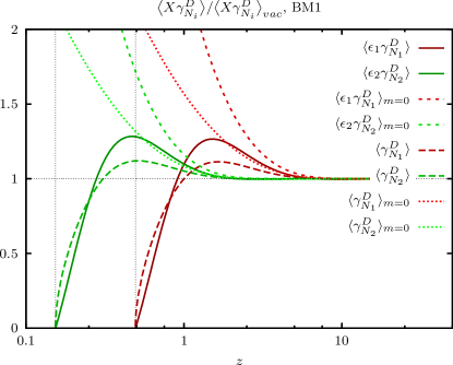
Figure 9: Decay and CP-violating reaction densities with thermal lepton and Higgs masses, ${\langle{X\gamma^{D}_{N_{i}}}\rangle}$, and with zero masses, ${\langle{X\gamma^{D}_{N_{i}}}\rangle_{m=0}}$, for the two Majorana neutrinos $N_{1}$ and $N_{2}$. The values are normalized to the corresponding reaction density in the conventional approximation ${\big{<}{X\gamma^{D}_{N_{i}}}\big{>}_{vac}}$. The thermal enhancement due to quantum-statistical factors is overcompensated by the phase space suppression due to thermal masses at high temperatures. Note that we show only the self-energy contribution to the CP-violating reaction densities.

However, the inclusion of the thermal masses turns this enhancement into a suppression at high temperatures. It is explained by the decrease of the decay phase space. At intermediate temperatures the thermal masses become small relative to the Majorana mass and we observe a minor enhancement. For the CP-violating reaction density we observe a very similar behavior. Given that for a hierarchical mass spectrum most of the asymmetry is typically generated by the lightest Majorana neutrino at $z_{f}\sim\ln K_{1}\sim{\cal O}(1)$, where $K_{1}$ is the washout parameter (see Appendix E), we expect the medium effects to induce a moderate enhancement of the total generated asymmetry.

VI.4 Majorana-mediated scattering

Two-body scattering processes mediated by Majorana neutrinos violate lepton number by two units and play an important role in the washout of the generated asymmetry. In this section we derive the effective scattering amplitudes using NEQFT. This is an important part of our results.

The last three terms in Eq. (VI.2) contain the Wigner-transformed one-loop Majorana self-energy:

$$\Pi^{ij}_{\gtrless}(t,q)= -g_{w}\int\,d\Pi^{4}_{k}\,d\Pi^{4}_{p}(2\pi)^{4}\delta(q-p-k)$$

$$\times\bigl{[}\,(h^{\dagger}h)_{ij}P_{L}S_{\gtrless}(t,p)P_{R}\Delta_{\gtrless}(t,k)$$

$$+(h^{\dagger}h)_{ji}P_{R}P\bar{S}_{\gtrless}(t,\bar{p})PP_{L}\bar{\Delta}_{\gtrless}(t,\bar{k})\bigr{]}{\,,}\hphantom{a}$$ (117)

see Appendix D.3 for more details. Combining them with Eq. (V.2) we find that their contribution to the divergence of the lepton-current (69) contains two Wightman propagators of leptons and two of the Higgs field. As we have argued above, these correspond to initial and final states in the kinetic equations. Therefore, we conclude that these terms describe scattering processes depicted in Fig. 2 and Fig. 3. As Higgs and leptons are maintained close to equilibrium we can safely use the Kadanoff-Baym ansatz for their propagators in the Majorana self-energy (VI.4). Inserting Eq. (VI.4) into the scattering terms of Eq. (VI.2) we can then split the Majorana propagator into a lepton number conserving and lepton number violating part:

$$\mathscr{S}^{ij}_{>}(q) =g_{w}\int\,d\Pi^{4}_{k}\,d\Pi^{4}_{p}(2\pi)^{4}\delta(q-p-k)\Delta_{\rho}(k)\mathbf{S}_{\rho}(p)$$

$$\times\big{[}(1-f_{\bar{\ell}}^{p})(1+f_{\bar{\phi}}^{k})\mathscr{S}^{ij}_{LC}(q,p)$$

$$+(1-f_{\bar{\ell}}^{p})(1+f_{\bar{\phi}}^{k})\mathscr{S}^{ij}_{LV}(q,p)\big{]}{\,,}$$ (118a)

$$\mathscr{S}^{ij}_{<}(q) =-g_{w}\int\,d\Pi^{4}_{k}\,d\Pi^{4}_{p}(2\pi)^{4}\delta(q-p-k)\Delta_{\rho}(k)\mathbf{S}_{\rho}(p)$$

$$\times\bigl{[}f_{\ell}^{p}f_{\phi}^{k}\mathscr{S}^{ij}_{LC}(q,p)+f_{\bar{\ell}}^{p}f_{\bar{\phi}}^{k}\mathscr{S}^{ij}_{LV}(q,p)\bigr{]}{\,,}$$ (118b)

where we have defined:

$$\mathscr{S}^{ij}_{LC}=(h^{\dagger}h)_{ij}\bigl{[}(1-\delta^{ij})\mathcal{S}^{ii}_{R}(q)P_{L}\not{p}P_{R}\mathcal{S}^{jj}_{A}(q)$$ (119a)

$$+\frac{\delta^{ij}}{2}\big{(}\mathcal{S}^{ii}_{R}(q)P_{L}\not{p}P_{R}\mathcal{S}^{jj}_{R}(q)+\mathcal{S}^{ii}_{A}(q)P_{L}\not{p}P_{R}\mathcal{S}^{jj}_{A}(q)\big{)}\bigr{]}{\,,}$$

$$\mathscr{S}^{ij}_{LV}=(h^{\dagger}h)_{ji}\bigl{[}(1-\delta^{ij})\mathcal{S}^{ii}_{R}(q)P_{R}\not{p}P_{L}\mathcal{S}^{jj}_{A}(q)$$ (119b)

$$+\frac{\delta^{ij}}{2}\big{(}\mathcal{S}^{ii}_{R}(q)P_{R}\not{p}P_{L}\mathcal{S}^{jj}_{R}(q)+\mathcal{S}^{ii}_{A}(q)P_{R}\not{p}P_{L}\mathcal{S}^{jj}_{A}(q)\big{)}\bigr{]}{\,.}$$

Here we neglected higher order terms coming from the matrices $\hat{\Theta}_{R}$ and $\hat{\Theta}_{A}$. The first terms in Eqs. (119a) and (119b) corresponds to the second term in Eq. (VI.2), whereas the remaining terms correspond to the last two terms in Eq. (VI.2). Substituting the Majorana propagators (118) into the lepton-current (69) together with the one-loop lepton self-energy (V.2) we finally obtain

$${\cal D}_{\mu}j^{\mu}_{L}(t) =g_{w}^{2}\int\!\,d\Pi^{4}_{p_{1}}\,d\Pi^{4}_{k_{1}}\,d\Pi^{4}_{p_{2}}\,d\Pi^{4}_{k_{2}}$$

$$\times\Delta_{\rho}(k_{1})\Delta_{\rho}(k_{2})\mathbf{S}_{\rho}(p_{1})\mathbf{S}_{\rho}(p_{2})$$

$$\times\bigl{[}A^{LV}(p_{1}+k_{1},p_{1},p_{2}){\mathcal{F}_{{\ell}\phi\leftrightarrow\bar{\ell}\bar{\phi}}^{p_{1}k_{1};p_{2}k_{2}}}$$

$$+A^{LC}(p_{1}+k_{1},p_{1},p_{2}){\mathcal{F}_{{\ell}\phi\leftrightarrow{\ell}\phi}^{p_{1}k_{1};p_{2}k_{2}}}\bigr{]}{\,.}$$ (120)

Note that the zeroth component of the momenta in the above equation can have both signs. The effective amplitudes of the lepton number conserving and lepton number violating processes read

$$A^{LV}(q,p_{1},p_{2})\equiv (h^{\dagger}h)_{ji}\,{\rm tr}\bigl{[}\mathscr{S}^{ij}_{LV}(q,p_{2})P_{L}\not{p}_{1}P_{R}\bigr{]}{\,,}\hphantom{aaaa}$$ (121a)

$$A^{LC}(q,p_{1},p_{2})\equiv (h^{\dagger}h)_{ji}\,{\rm tr}\bigl{[}\mathscr{S}^{ij}_{LC}(q,p_{2})P_{L}\not{p}_{1}P_{R}\bigr{]}{\,.}\hphantom{aaaa}$$ (121b)

The functions $A^{LC}(q,p_{1},p_{2})$ and $A^{LV}(q,p_{1},p_{2})$ are symmetric under the exchange of the momenta $p_{1}$ and $p_{2}$. This implies that the contribution of $A^{LC}$ in Eq. (VI.4) vanishes. The terms of $\mathscr{S}_{LV}$ diagonal in flavor space correspond to the RIS-propagator. Substituting Eq. (VI.2) into Eq. (121a) and taking the trace we find that it contains only the scalar components of the retarded and advanced propagators and is proportional to:

$$\boldsymbol{\mathcal{S}}^{2}_{R}+\boldsymbol{\mathcal{S}}^{2}_{A} \approx 2M^{2}\frac{{\boldsymbol{\Omega}}^{2}_{h}-{\boldsymbol{\Pi}}^{2}_{\rho}}{\left[{\boldsymbol{\Omega}}^{2}_{h}+{\boldsymbol{\Pi}}^{2}_{\rho}\right]^{2}}$$

$$\approx 2M^{2}\frac{(q^{2}-M^{2})^{2}-(M{\boldsymbol{\Gamma}})^{2}}{\left[(q^{2}-M^{2})^{2}+(M{\boldsymbol{\Gamma}})^{2}\right]^{2}}{\,.}$$ (122)

Equation (VI.4) differs from the canonical result (20) only in that the vacuum masses and decay widths are replaced by thermal ones. For a hierarchical mass spectrum this difference can be safely neglected. Introducing an analogue of the RIS subtracted propagator,

$$\mathscr{P}_{ij}(q)\equiv\boldsymbol{\mathcal{S}}^{ii}_{A}(q)\boldsymbol{\mathcal{S}}^{jj}_{R}(q)-{\textstyle\frac{1}{2}}\delta^{ij}\boldsymbol{\mathcal{S}}^{ii}_{\rho}(q)\boldsymbol{\mathcal{S}}^{ii}_{\rho}(q){\,,}$$ (123)

we can rewrite the lepton number violating effective amplitude in a compact form:

$$A^{LV}(q,p_{1},p_{2}) =2(h^{\dagger}h)_{ij}^{2}(p_{1}p_{2})M_{i}M_{j}\mathscr{P}_{ij}(q){\,.}$$

Next we perform the trivial integrations over the frequencies using the Dirac-deltas in the quasiparticle spectral functions (V.2) and (80). Each Dirac-delta can be decomposed into two terms, one with positive and one with negative frequency. Therefore, the integration over the four frequencies gives rise to $2^{4}$ terms, but only six of them satisfy energy conservation ensured by the remaining delta-function. In a homogeneous and isotropic medium the one-particle distribution functions satisfy

$$1-f_{\ell}(-p)=f_{\bar{\ell}}(p){\,,}\quad 1+f_{\phi}(-k)=-f_{\bar{\phi}}(k){\,,}$$ (124)

and the diagonal Majorana propagators have the properties

$$\boldsymbol{\mathcal{S}}^{ii}_{\rho}(-q)=-\boldsymbol{\mathcal{S}}^{ii}_{\rho}(q){\,,}\quad\boldsymbol{\mathcal{S}}^{ii}_{R}(-q)=\boldsymbol{\mathcal{S}}^{ii}_{A}(q){\,.}$$ (125)

Upon substitution of the resulting self-energy into Eq. (69) and the use of Eqs. (124) and (125) the remaining six contributions in the lepton-current can be conveniently written as

$${\cal D}_{\mu}j_{L}^{\mu}(t)\Big{|}_{S}^{S}= -\int{\,d\Pi_{{\ell}{\ell}\phi\phi}^{p_{1}p_{2}k_{1}k_{2}}}$$

$$\times\Big{[}\Xi^{(t\times t)}_{\bar{\phi}\bar{\phi}\leftrightarrow{\ell}{\ell}}{\mathcal{F}_{\bar{\phi}\bar{\phi}\leftrightarrow{\ell}{\ell}}^{k_{1}k_{2};p_{1}p_{2}}}+\Xi^{(t\times t)}_{\bar{\ell}\bar{\ell}\leftrightarrow\phi\phi}{\mathcal{F}_{\bar{\ell}\bar{\ell}\leftrightarrow\phi\phi}^{p_{1}p_{2};k_{1}k_{2}}}$$

$$+2\big{(}\Xi^{(s\times s)}_{\bar{\ell}\bar{\phi}\leftrightarrow{\ell}\phi}+\Xi^{(t\times t)}_{\bar{\ell}\bar{\phi}\leftrightarrow{\ell}\phi}\big{)}{\mathcal{F}_{\bar{\ell}\bar{\phi}\leftrightarrow{\ell}\phi}^{p_{1}k_{1};p_{2}k_{2}}}\Big{]}{\,,}$$ (126)

where we have defined the effective scattering amplitudes:

$$\Xi^{(s\times s)}_{\bar{\ell}\bar{\phi}\leftrightarrow{\ell}\phi} =2g_{w}^{2}(p_{1}p_{2})\sum\Re(h^{\dagger}h)_{ij}^{2}M_{i}M_{j}\mathscr{P}_{ij}(q_{s}){\,,}\hphantom{aaaa}$$ (127a)

$$\Xi^{(t\times t)}_{\bar{\ell}\bar{\phi}\leftrightarrow{\ell}\phi} =2g_{w}^{2}(p_{1}p_{2})\sum\Re(h^{\dagger}h)_{ij}^{2}M_{i}M_{j}\mathscr{P}_{ij}(q_{t}){\,,}$$ (127b)

$$\Xi^{(t\times t)}_{\bar{\ell}\bar{\ell}\leftrightarrow\phi\phi} =2g_{w}^{2}(p_{1}p_{2})\sum(h^{\dagger}h)_{ij}^{2}M_{i}M_{j}\mathscr{P}_{ij}(q_{t}){\,,}$$ (127c)

$$\Xi^{(t\times t)}_{\bar{\phi}\bar{\phi}\leftrightarrow{\ell}{\ell}} =2g_{w}^{2}(p_{1}p_{2})\sum(h^{\dagger}h)_{ji}^{2}M_{i}M_{j}\mathscr{P}_{ij}(q_{t}){\,.}$$ (127d)

The momenta of the Majorana neutrinos are related to the momenta of the initial and final states by $q_{s}=p_{1}+k_{1}$ and $q_{t}=p_{1}-k_{2}$. From Eq. (127) we see that the obtained amplitudes contain only $s\times s$ and $t\times t$ interference terms. Indeed, in the products of the Majorana propagators in Eq. (123) both of them depend on the same momentum.

The missing cross terms emerge from the two-loop (vertex) contribution to the lepton self-energy. As we have mentioned in Sec. V, within the discussed assumptions and approximations the second and third terms on the right-hand side of Eq. (73) describe scattering processes. Since they are of the fourth order in the Yukawas, we can replace the full Majorana propagators by the diagonal propagators. The third term, Eq. (V.2), corresponds to lepton number conserving processes and does not need to be discussed further. The second one, Eq. (V.2), is given by

$$\Sigma^{(2.2)}_{\gtrless} (t,p)=\int\,d\Pi^{4}_{p_{2}}\,d\Pi^{4}_{k_{1}}\,d\Pi^{4}_{k_{2}}(2\pi)^{4}\delta(p+k_{1}-p_{2}-k_{2})$$

$$\times (h^{\dagger}h)^{2}_{ij}\bigl{[}P_{R}\mathcal{S}^{jj}_{R}(t,p_{2}+k_{2})CP_{R}S^{T}_{\lessgtr}(t,-p_{2})P_{L}$$

$$\times C\mathcal{S}^{ii}_{A}(t,p_{2}-k_{1})P_{L}\Delta_{\lessgtr}(t,k_{1})\Delta_{\lessgtr}(t,-k_{2})\bigr{]}{\,.}$$ (128)

We substitute Eq. (VI.4) into the equation for the lepton-current (69) and perform the steps preceding Eq. (VI.4). Using furthermore relations (124) we find

$${\cal D}_{\mu}j^{\mu}_{L}(t)\Big{|}_{S}^{V}= -\int{\,d\Pi_{{\ell}\phi{\ell}\phi}^{p_{1}k_{1}p_{2}k_{2}}}$$

$$\times\Bigl{[}2\Xi^{(s\times t)}_{\bar{\ell}\bar{\phi}\leftrightarrow{\ell}\phi}{\mathcal{F}_{\bar{\ell}\bar{\phi}\leftrightarrow{\ell}\phi}^{p_{1}k_{1};p_{2}k_{2}}}+\Xi^{(u\times t)}_{\bar{\phi}\bar{\phi}\leftrightarrow{\ell}{\ell}}{\mathcal{F}_{\bar{\phi}\bar{\phi}\leftrightarrow{\ell}{\ell}}^{k_{1}k_{2};p_{1}p_{2}}}$$

$$+\Xi^{(u\times t)}_{\bar{\ell}\bar{\ell}\leftrightarrow\phi\phi}{\mathcal{F}_{\bar{\ell}\bar{\ell}\leftrightarrow\phi\phi}^{p_{1}p_{2};k_{1}k_{2}}}\Bigr{]}{\,,}$$ (129)

where we have introduced

$$\Xi^{(s\times t)}_{\bar{\ell}\bar{\phi}\leftrightarrow{\ell}\phi} \equiv 4g_{w}(p_{1}p_{2})\sum M_{i}M_{j}\Re\,(h^{\dagger}h)_{ij}^{2}$$

$$\times\Re\,\bigl{\{}\boldsymbol{\mathcal{S}}^{ii}_{A}(q_{t})\boldsymbol{\mathcal{S}}^{jj}_{R}(q_{s})\bigr{\}}{\,,}$$ (130a)

$$\Xi^{(u\times t)}_{\bar{\ell}\bar{\ell}\leftrightarrow\phi\phi} \equiv 2g_{w}(p_{1}p_{2})\sum M_{i}M_{j}$$

$$\times\Re\bigl{\{}(h^{\dagger}h)_{ij}^{2}\,\boldsymbol{\mathcal{S}}^{ii}_{A}(q_{t})\boldsymbol{\mathcal{S}}^{jj}_{R}(q_{u})\bigr{\}}{\,,}$$ (130b)

$$\Xi^{(u\times t)}_{\bar{\phi}\bar{\phi}\leftrightarrow{\ell}{\ell}} \equiv 2g_{w}(p_{1}p_{2})\sum M_{i}M_{j}$$

$$\times\Re\bigl{\{}(h^{\dagger}h)_{ji}^{2}\,\boldsymbol{\mathcal{S}}^{ii}_{A}(q_{u})\boldsymbol{\mathcal{S}}^{jj}_{R}(q_{t})\bigr{\}}{\,,}$$ (130c)

and $q_{u}=p_{2}-k_{2}$. The combinations of the momenta appearing in the products of the Majorana propagators clearly indicate that the above amplitudes correspond to the interference terms of the $s$-, $t$-, and $u$-channel contributions.

Combining Eqs. (127) and (130) we obtain for the effective amplitude of ${\ell}{\ell}\leftrightarrow\bar{\phi}\bar{\phi}$ scattering:

$$\Xi_{{\ell}{\ell}\leftrightarrow\bar{\phi}\bar{\phi}} =2(p_{1}p_{2})\sum(h^{\dagger}h)^{2}_{ij}M_{i}M_{j}$$

$$\times\bigl{[}4\mathscr{P}_{ij}(q_{t})$$

$$+\boldsymbol{\mathcal{S}}^{ii}_{A}(q_{t})\boldsymbol{\mathcal{S}}^{jj}_{R}(q_{u})+\boldsymbol{\mathcal{S}}^{ii}_{A}(q_{u})\boldsymbol{\mathcal{S}}^{jj}_{R}(q_{t})\bigr{]}{\,,}$$ (131)

whereas the effective amplitude of ${\ell}\phi\leftrightarrow\bar{\ell}\bar{\phi}$ scattering reads

$$\Xi_{{\ell}\phi\leftrightarrow\bar{\ell}\bar{\phi}} =4(p_{1}p_{2})\sum\Re(h^{\dagger}h)^{2}_{ij}M_{i}M_{j}$$

$$\times\bigl{[}2\mathscr{P}_{ij}(q_{s})+2\mathscr{P}_{ij}(q_{t})$$

$$+\boldsymbol{\mathcal{S}}^{ii}_{A}(q_{t})\boldsymbol{\mathcal{S}}^{jj}_{R}(q_{s})+\boldsymbol{\mathcal{S}}^{ii}_{A}(q_{s})\boldsymbol{\mathcal{S}}^{jj}_{R}(q_{t})\bigr{]}{\,.}$$ (132)

To compare the obtained expressions with the vacuum results of the canonical computation Eqs. (II) and (II), we evaluate the retarded and advanced propagators at zero temperature. In vacuum $L_{\rho}(t,q)=\theta(q^{2})\,\mathrm{sign}(q^{0})\,\not{q}$. Therefore for positive $q_{0}$ it follows from Eq. (95) that

$$\boldsymbol{\mathcal{S}}^{ii}_{R/A}(q)\approx-\left[q^{2}-M_{i}^{2}\pm i\theta(q^{2})\Gamma_{i}/M_{i}\,q^{2}\right]^{-1}{\,.}$$ (133)

In the vicinity of the mass shell of the respective Majorana neutrino $q^{2}=M_{i}^{2}$ and we find

$$\boldsymbol{\mathcal{S}}^{ii}_{R}=-P_{i}{\,,}\quad\boldsymbol{\mathcal{S}}^{ii}_{A}=-P^{*}_{i}{\,.}$$ (134)

For $t$- and $u$-channels the imaginary parts of Eqs. (13) and (133) vanish, so that in the vacuum limit

$$\mathscr{P}_{ij}(q)=P^{*}_{i}(q^{2})P_{j}(q^{2}){\,,}$$ (135)

and $\mathscr{P}_{ij}$ is symmetric with respect to $i\leftrightarrow j$. The squares of the $t$- and $u$-channel propagators in Eq. (II) give identical contributions to the reduced cross section of ${\ell}{\ell}\leftrightarrow\bar{\phi}\bar{\phi}$ process. Therefore, upon substitution of Eq. (VI.4) into Eq. (57) and the use of the $i\leftrightarrow j$ symmetry, we recover for the reduced cross section the canonical result (58). Relations (134) imply that the off-diagonal components of $\mathcal{P}_{ij}$ and $\mathscr{P}_{ij}$ coincide. For the $s$-channel the diagonal components of $\mathscr{P}_{ii}$ are given in the vacuum limit by

$$\mathscr{P}_{ii}(q_{s})=\frac{(s-M_{i}^{2})^{2}-(\Gamma_{i}/M_{i}\,s)^{2}}{[(s-M_{i}^{2})^{2}+(\Gamma_{i}/M_{i}\,s)^{2}]^{2}}{\,.}$$ (136)

Thus, in the vicinity of the mass shell, $s\approx M_{i}^{2}$, the canonical expression for the RIS-subtracted propagator, Eq. (20), coincides with the expression obtained from first principles. This justifies results of the earlier calculations. For the reduced cross section of ${\ell}\phi\leftrightarrow\bar{\ell}\bar{\phi}$ scattering we recover Eq. (59).

At finite temperatures $L_{\rho}(t,\not{q})$ is not zero even for $t$- and $u$-channels. In other words, the medium effects induce additional contributions to the effective decay amplitudes. However, these contributions are proportional to the coefficients $c_{i}$. Numerical analysis shows that for the two chosen sets of parameters, see Appendix E, the additional correction typically do not have any sizable impact on the reaction densities.

A quantity relevant for the numerical analysis is the ratio $z\langle\gamma_{ij}^{ab}\rangle/{\cal H}s$. The dependence of this ratio on the dimensionless inverse temperature is presented in Fig. 10 and Fig. 11. If the approximate expression (56) is used, then the reaction density of ${\ell}\phi\leftrightarrow\bar{\ell}\bar{\phi}$ scattering becomes negative for $2\lesssim z\lesssim 3$ for the first set of the parameters whereas for the second set of the parameters it turns negative for $0.5\lesssim z\lesssim 1$. A qualitatively similar behavior has also been observed in Pilaftsis and Underwood (2004).

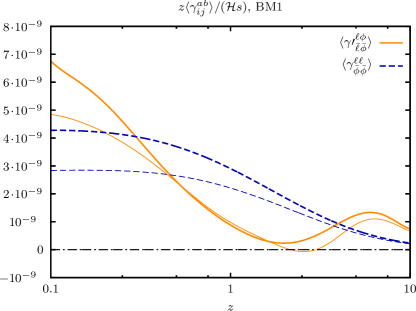
Figure 10: Washout reaction densities due to ${\ell}{\ell}\leftrightarrow\bar{\phi}\bar{\phi}$ and ${\ell}\phi\leftrightarrow\bar{\ell}\bar{\phi}$ scattering processes for benchmark point 1 in the approximation of massless leptons and Higgs. Shown are the reaction densities computed using the Boltzmann approximation (56) (thin lines), and taking into account the quantum-statistical effects, (IV) (thick lines). The (RIS subtracted) reaction densities $\langle\gamma^{\prime{\ell}\phi}_{\bar{{\ell}}\bar{\phi}}\rangle$ may be negative as they are not the physical rates for the $2\leftrightarrow 2$ scattering process.

This rather counter-intuitive result can be traced back to the behavior of the RIS part of the effective amplitude (II) which is negative in the vicinity of the mass shell. Its sign is not fixed by physical requirements, since it constitutes a sub-leading contribution to the washout rate.

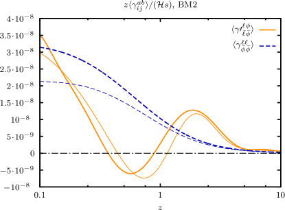
Figure 11: Washout reaction densities due to ${\ell}{\ell}\leftrightarrow\bar{\phi}\bar{\phi}$ and ${\ell}\phi\leftrightarrow\bar{\ell}\bar{\phi}$ scattering processes for benchmark point 2. Compare Fig. 10.

As can be inferred from Fig. 10, for the first set of model parameters the quantum-statistical corrections render the RIS subtracted reaction density of ${\ell}\phi\leftrightarrow\bar{\ell}\bar{\phi}$ scattering positive in the whole range of temperatures. However, this is merely a numerical coincidence. For the second set of parameters, see Fig. 11, the reaction density of ${\ell}\phi\leftrightarrow\bar{\ell}\bar{\phi}$ scattering remains negative for $0.4\lesssim z\lesssim 0.9$. It is nevertheless important to note that even in the region where the reaction density is negative the quantum-statistical corrections shift it upwards as compared to the result of the canonical computation.

As far as $\bar{\ell}\bar{\ell}\leftrightarrow\phi\phi$ scattering is concerned, the quantum-statistical corrections enhance the reduced reaction density at high temperatures by about 50%. As the temperature decreases, the reaction density computed using Eq. (IV) approaches the one computed using Eq. (56) as one would expect. A similar behavior is also observed for the reaction density of ${\ell}\phi\leftrightarrow\bar{\ell}\bar{\phi}$ scattering.

In Figs. 10 and 11 we neglected the thermal masses of initial and final states.

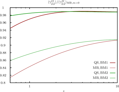
Figure 12: Ratio of the reaction density computed using thermal masses with (thick lines) and without (thin lines) the quantum-statistical terms to the canonical one for the two sets of parameters.

To estimate the size of the mass corrections, in Fig. 12 we plot ratio of the reaction density of the ${\ell}{\ell}\leftrightarrow\bar{\phi}\bar{\phi}$ scattering computed using thermal masses of the Higgs and leptons with and without the quantum-statistical terms to the canonical one for the two sets of parameters. If the quantum-statistical effects are neglected, the thermal masses lead to a $\sim 15\%$ suppression of the reaction densities. On the other hand, an enhancement induced by the quantum-statistical terms to a large extent compensates the mass-induced suppression. As a result, the deviation from the canonical reaction density does not exceed $\sim 5\%$ in the whole range of temperatures.

To compare the relative importance of the (inverse) decay and scattering processes in Fig. 13 and Fig. 14 we also present the uniformly normalized reaction densities.

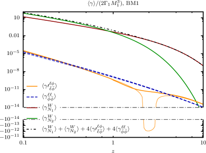
Figure 13: Washout reaction densities due to ${\ell}{\ell}\leftrightarrow\bar{\phi}\bar{\phi}$ and ${\ell}\phi\leftrightarrow\bar{\ell}\bar{\phi}$ scattering processes for benchmark point 1 in the approximation of massless leptons and Higgs. For comparison the washout reaction densities for $N_{1}$ and $N_{2}$ (inverse) decays are shown as well. Note that the normalization differs from the one used in Fig. 10 and Fig. 11 For the present choice of parameters contributions by $2\leftrightarrow 2$ scatterings are strongly suppressed by the smallness of the couplings.

In both cases we observe a qualitatively similar picture: for the chosen sets of parameters reaction densities of the scattering processes are strongly suppressed by the smallness of the Yukawa couplings as compared to those of the decay processes.

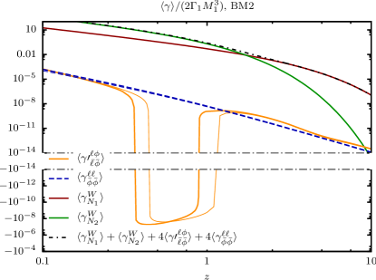
Figure 14: Washout reaction densities due to ${\ell}{\ell}\leftrightarrow\bar{\phi}\bar{\phi}$ and ${\ell}\phi\leftrightarrow\bar{\ell}\bar{\phi}$ scattering processes as well as (inverse) decays for benchmark point 2. Compare Fig. 13.

In the rate equation for the lepton asymmetry, see Eq. (37a), the total washout rate is given by a sum of reaction densities for decays and scattering. Whereas $\langle\gamma^{W}_{N_{i}}\rangle$ and $\langle\gamma^{{\ell}{\ell}}_{\bar{\phi}\bar{\phi}}\rangle$ are positive, the RIS subtracted reaction density $\langle\gamma^{\prime{\ell}\phi}_{\bar{\ell}\bar{\phi}}\rangle$ can be negative at some temperatures. If the total washout rate would turn negative, it would lead to a spurious self-enhanced generation of the asymmetry. In Figs. 13 and 14 we show the sum of the reactions densities. For both parameter sets it is positive. This sum should always be positive. If the quantum-statistical terms are neglected this can be demonstrated explicitly. In the absence of the quantum-statistical corrections, the results of this section revert to the ones discussed in Sec. II. Using the expression for the RIS-propagator, Eq. (21), we can rewrite the RIS subtracted scattering amplitude (II) as a difference of the unsubtracted one and the RIS term. Since the latter is proportional to $\delta(s-M_{i}^{2})$ the integration in Eqs. (57) and (56) is trivial and we obtain after some algebra:

$$4\langle\gamma^{\prime{\ell}\phi}_{\bar{\ell}\bar{\phi}}\rangle\approx 4\langle\gamma^{{\ell}\phi}_{\bar{\ell}\bar{\phi}}\rangle-{\textstyle\sum_{i}}\langle\gamma^{W}_{N_{i}}\rangle{\,.}$$ (137)

The total washout rate is then given by $4\langle\gamma^{{\ell}\phi}_{\bar{\ell}\bar{\phi}}\rangle+4\langle\gamma^{{\ell}{\ell}}_{\bar{\phi}\bar{\phi}}\rangle$ and is positive as a sum of two positive functions. In other words, even though $\langle\gamma^{\prime{\ell}\phi}_{\bar{\ell}\bar{\phi}}\rangle$ can be negative at some temperatures, the total washout rate is always positive. The form of the unsubtracted scattering reaction density that can be inferred from Eq. (137) is another manifestation of the double-counting. If we had not subtracted the RIS contribution, we would have counted contributions of the inverse decay processes twice and ended up with an incorrect prediction for the generated asymmetry.

VII Higgs contribution

In the preceding section we have approximately taken the gauge interactions into account in the form of effective masses of the Higgs and leptons. The thermal masses are of order of $gT$ and large enough to influence the values of the reaction densities quantitatively. In particular, the Majorana neutrino decay can become kinematically forbidden when the sum of the masses of lepton and Higgs exceeds the heavy Majorana neutrino mass. For even higher temperatures (with $m_{\phi}(T)>m_{{\ell}}(T)+{M_{i}}(T)$) the Higgs decay channel into a lepton-Majorana pair becomes kinematically allowed instead and can contribute to the asymmetry since it violates CP. For simplicity we do not take modified dispersion relations into account here, see Weldon (1989); Giudice et al. (2004); Kießig et al. (2010a); Kießig and Plümacher (2012a, b), but use the simple picture of temperature dependent thermal masses as an estimate:

$$m_{\phi}^{2} =\bigg{(}\frac{3}{16}g_{2}^{2}+\frac{1}{16}g^{\prime 2}+\frac{1}{4}h_{t}^{2}+\frac{1}{2}\lambda\bigg{)}{T^{2}},$$

$$m_{{\ell}}^{2} =\bigg{(}\frac{3}{32}g_{2}^{2}+\frac{1}{32}g^{\prime 2}\bigg{)}{T^{2}}{\,,}$$ (138)

where we use the temperature dependent values of the $SU(2)_{L}$, $U(1)$, top Yukawa and Higgs self-couplings $g_{2}$, $g^{\prime}$, $h_{t}$ and $\lambda$ assuming a Higgs mass of $115\,\mathrm{GeV}$ Kajantie et al. (1996). We also ignore that the thermal mass of leptons might be better approximated by the ‘asymptotic thermal mass’ $\sqrt{2}m_{{\ell}}$ in a kinematic regime in which their momentum is such that $p^{2}\sim(gT)^{2}$ Weldon (1982). We do also not take into account, in our quantitative analysis, the thermal corrections to the Majorana neutrino masses as they are negligible compared to their vacuum masses.

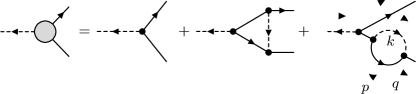
Figure 15: Tree level contribution and one-loop corrections to the (anti-)Higgs decay amplitude. The additional arrows illustrate the direction of momentum flow.

The CP-violating decay of the Higgs arises from the interference of the tree-level, self-energy and vertex graphs depicted in Fig. 15. Although in this case the decaying particle – the Higgs doublet – is very close to thermal equilibrium due to the Yukawa and gauge interactions of the Standard Model, the Majorana neutrino in the final state may deviate from equilibrium, so that the third Sakharov condition is fulfilled.

Using the expression for the divergence of the lepton-current, Eq. (69), we can extract the corresponding CP-violating parameter. To calculate the self-energy contribution it is convenient to rewrite the one-loop lepton self-energy (V.2) in the form:

$$\Sigma_{\gtrless}(t,p) =-(h^{\dagger}h)_{ji}{\textstyle\int}\,d\Pi^{4}_{k}\,d\Pi^{4}_{q}(2\pi)^{4}\delta(q+p-k)$$

$$\times\bar{\Delta}_{\gtrless}(t,\bar{k})P_{R}C(\mathscr{S}^{ji}_{\lessgtr})^{T}(t,q)C^{-1}P_{L}{\,,}$$ (139)

where the transposition is only in Dirac space and we have used one of the properties of Majorana propagator:

$$(\mathscr{S}^{ij}_{\gtrless})(X,q)=C(\mathscr{S}^{ji}_{\lessgtr})^{T}(X,-q)C^{-1}{\,.}$$ (140)

In its CP conjugate the Yukawa couplings are replaced by their complex conjugates and the propagators by the CP conjugate ones.

Similar to the case of the Majorana decay, substituting Eq. (VII) into Eq. (69) we can define effective Higgs decay amplitudes:

$$\Xi_{\bar{\phi}\leftrightarrow{\ell}N_{i}} \equiv g_{w}\sum_{mn}(h^{\dagger}h)_{mn}$$

$$\times{\rm tr}\left[\Theta^{mi}_{R}(q)(\not{q}+M_{i})\Theta^{in}_{A}(q)P_{R}\not{p}P_{L}\right]{\,,}\hphantom{aa}$$ (141a)

$$\Xi_{\phi\leftrightarrow\bar{\ell}N_{i}} \equiv g_{w}\sum_{mn}(h^{\dagger}h)^{*}_{mn}$$

$$\times{\rm tr}\left[\bar{\Theta}^{mi}_{R}(q)(\not{q}+M_{i})\bar{\Theta}^{in}_{A}(q)P_{R}\not{p}P_{L}\right]{\,.}$$ (141b)

The overall factor $g_{w}$ in Eqs. (141) comes from summation over the doublet components of the (decaying) Higgs particle. To leading order in the couplings:

$$\Xi_{\bar{\phi}\leftrightarrow{\ell}N_{i}} \approx 2g_{w}\bigl{[}(h^{\dagger}h)_{ii}(p\cdot q)$$

$$+{\textstyle\frac{g_{w}}{16\pi}}\Im(h^{\dagger}h)_{ij}^{2}M_{i}M_{j}\boldsymbol{\mathcal{S}}^{jj}_{h}(p\,L_{\rho})\bigr{]}{\,,}$$ (142a)

$$\Xi_{\phi\leftrightarrow\bar{\ell}N_{i}} \approx 2g_{w}\bigl{[}(h^{\dagger}h)_{ii}(p\cdot q)$$

$$-{\textstyle\frac{g_{w}}{16\pi}}\Im(h^{\dagger}h)_{ij}^{2}M_{i}M_{j}\boldsymbol{\mathcal{S}}^{jj}_{h}(p\,L_{\rho})\bigr{]}{\,,}$$ (142b)

which, up to the relative sign in square brackets, coincides with the amplitudes (105). The corresponding CP-violating parameter reads

$$\epsilon_{\phi,i}^{S}=-\frac{\Im(h^{\dagger}h)^{2}_{ij}}{(h^{\dagger}h)_{ii}(h^{\dagger}h)_{jj}}\frac{M_{i}\Gamma_{j}}{M_{i}^{2}-M_{j}^{2}}\frac{pL_{\rho}}{pq}{\,,}$$ (143)

where $p$ and $q$ are the momenta of the on-shell final lepton and Majorana neutrino with positive zeroth components respectively. The direction of momentum flow is as defined in Fig. 15. Although $L_{\rho}$ in Eqs. (VI.3) and (143) is one and the same function, because of the different kinematic regimes the explicit result in terms of the distribution functions differs for the Higgs decay:

$$L_{\rho}(t,q)=16\pi\int \,d\Pi^{\phi}_{k}\,d\Pi^{{\ell}}_{p}(2\pi)^{4}\delta(q+p-k)\,\not{p}$$

$$\times [\,f_{\phi}(E_{k})+f_{\ell}(E_{p})]{\,,}$$ (144)

see Appendix D.3. Note that our result is different from the one presented in Covi et al. (1998); Giudice et al. (2004); Davidson et al. (2008). Instead of the $f_{\phi}-f_{{\ell}}-2f_{\phi}f_{{\ell}}$ dependence, it is proportional to a sum, $f_{\phi}+f_{\ell}$, of the two distribution functions. This dependence can also be obtained in the framework of real time thermal field theory using causal $n$-point functions, compare Garny et al. (2010b). The derivation within the Kadanoff-Baym formalism gives certainty concerning the sign of the contribution by Higgs decay. The CP-violating parameter (143) has an opposite sign relative to that for Majorana neutrino decay. However, it is canceled by the relative sign in Eq. (VII).

To calculate the vertex contribution we use Eq. (140) and represent the two-loop self-energy (VI.3) in the form

$$\Sigma^{(2.1)}_{\gtrless}(t,p)=\int\,d\Pi^{4}_{q}\,d\Pi^{4}_{k}\ (2\pi)^{4}\delta(p+q-k)$$ (145)

$$\times\big{[}(h^{\dagger}h)^{2}_{ij}\varLambda_{jj}(t,-q,-k)P_{L}(\tilde{\mathcal{S}}^{ii}_{\lessgtr})^{T}(t,q)CP_{L}\bar{\Delta}_{\gtrless}(t,\bar{k})$$

$$+(h^{\dagger}h)^{2}_{ji}P_{R}C(\tilde{\mathcal{S}}^{ii}_{\lessgtr})^{T}(t,q)P_{R}V_{jj}(t,-q,-p)\bar{\Delta}_{\gtrless}(t,k)\big{]}{\,.}$$

Its CP conjugate again differs by the conjugation of the Yukawas and propagators. Substituting Eq. (145) and its CP conjugate into Eq. (69) we obtain for the corresponding effective amplitudes:

$$\Xi^{V}_{\bar{\phi}\leftrightarrow{\ell}N_{i}}\equiv g_{w}(h^{\dagger}h)_{ij}^{2}\ M_{i}\,{\rm tr}\bigl{[}\varLambda_{jj}(-q,-k)CP_{L}\not{p}P_{R}\bigr{]}$$

$$\hskip 8.53581pt+g_{w}(h^{\dagger}h)_{ji}^{2}\,M_{i}\,{\rm tr}\bigr{[}CV_{jj}(-q,-k)P_{L}\not{p}P_{R}\bigr{]}{\,,}$$ (146a)

$$\Xi^{V}_{\phi\leftrightarrow\bar{\ell}N_{i}}\equiv g_{w}(h^{\dagger}h)_{ij}^{2}\ M_{i}{\rm tr}\bigr{[}CV_{jj}(-q,-k)P_{L}\not{p}P_{R}\bigr{]}$$

$$\hskip 8.53581pt+g_{w}(h^{\dagger}h)_{ji}^{2}\,M_{i}{\rm tr}\bigl{[}\varLambda_{jj}(-q,-k)CP_{L}\not{p}P_{R}\bigr{]}{\,.}$$ (146b)

Just like for the self-energy contribution we observe that the overall sign of the vertex contribution to the Higgs decay amplitude is opposite to that in the Majorana decay, compare Eqs. (110) and (146). The corresponding CP-violating parameter reads

$$\epsilon_{\phi,i}^{V} =\sum\frac{\Im\,(h^{\dagger}h)_{ij}^{2}}{(h^{\dagger}h)_{ii}}\frac{M_{i}M_{j}}{qp}\ \int\,d\Pi^{4}_{k_{1}}\,d\Pi^{4}_{k_{2}}\,d\Pi^{4}_{k_{3}}$$ (147)

$$\times(2\pi)^{4}\delta(q-k_{1}-k_{2})(2\pi)^{4}\delta(k-k_{2}-k_{3})(pk_{2})$$

$$\times\bigl{[}\Delta_{\rho}(k_{1})\mathbf{S}_{F}(k_{2})\boldsymbol{\mathcal{S}}^{jj}_{h}(k_{3})+\Delta_{F}(k_{1})\mathbf{S}_{\rho}(k_{2})\boldsymbol{\mathcal{S}}^{jj}_{h}(k_{3})$$

$$-\Delta_{h}(k_{1})\mathbf{S}_{\rho}(k_{2})\boldsymbol{\mathcal{S}}^{jj}_{F}(k_{3})-\Delta_{h}(k_{1})\mathbf{S}_{F}(k_{2})\boldsymbol{\mathcal{S}}^{jj}_{\rho}(k_{3})$$

$$+\Delta_{\rho}(k_{1})\mathbf{S}_{h}(k_{2})\boldsymbol{\mathcal{S}}^{jj}_{F}(k_{3})-\Delta_{F}(k_{1})\mathbf{S}_{h}(k_{2})\boldsymbol{\mathcal{S}}^{jj}_{\rho}(k_{3})\bigr{]}{\,.}$$

The last three lines of Eq. (147) correspond to the three possible cuts of the vertex graph. Similarly to the Majorana decay only two of the intermediate states can be on-shell and for only one of them the corresponding distribution function enters the result. The value of the vertex CP-violating parameter depends on the temperature as well as on masses of the Majorana neutrinos. For definiteness, let us assume a strongly hierarchical mass spectrum, $M_{j}\gg m_{\phi}>M_{i}$. In this case contribution of the last two lines in Eq. (147) is strongly suppressed. Integrating out the delta-functions we find for the contribution of the first cut:

$$\epsilon_{\phi,i}^{V}=\frac{1}{2}\sum\frac{\Im\,(h^{\dagger}h)_{ij}^{2}}{(h^{\dagger}h)_{ii}(h^{\dagger}h)_{jj}} \frac{M_{i}\Gamma_{j}}{M^{2}_{j}}\frac{pK_{j}}{qp}{\,,}$$ (148)

where the loop function $K_{j}$ is now defined as:

$$K^{\mu}_{i}(q,k) =16\pi\int\,d\Pi^{\phi}_{k_{2}}\,d\Pi^{{\ell}}_{p_{2}}(2\pi)^{4}\delta(q+p_{2}-k_{2})\,p^{\mu}_{2}$$

$$\times\bigl{[}f_{\phi}(E_{k_{2}})+f_{{\ell}}(E_{p_{2}})\bigr{]}M_{i}^{2}\boldsymbol{\mathcal{S}}^{ii}_{h}(k-p_{2}){\,.}$$ (149)

Note that the vertex CP-violating parameter (148) has an opposite sign relative to that for Majorana neutrino decay. Similarly to the self-energy contribution we observe that the $1-f_{{\ell}}+f_{\phi}$ combination is replaced in (VII) by $f_{{\ell}}+f_{\phi}$. For a milder mass hierarchy the two other cuts can become important. Their contributions are proportional to $1-f_{{\ell}}-f_{N}$ and $f_{\phi}+f_{N}$ respectively.

The first-principle computation gives for the Higgs decay contribution to the evolution of the lepton current an expression similar to Eq. (32):

$$\frac{dY_{Li\atop N_{i}}}{dz} =\frac{z}{s{\cal H}}\int{\,d\Pi_{N_{i}\phi{\ell}}^{qkp}}$$

$$\times\bigl{[}\Xi_{\bar{\phi}\rightarrow{\ell}N_{i}}{\mathcal{F}_{N_{i}{\ell}\leftrightarrow\bar{\phi}}^{qp;k}}\mp\Xi_{\phi\rightarrow\bar{\ell}N_{i}}{\mathcal{F}_{N_{i}\bar{{\ell}}\leftrightarrow{\phi}}^{qp;k}}\bigr{]}{\,.}$$ (150)

We do not discuss ‘extra’ terms here which would arise from ‘naive’ Boltzmann equations. To write this as a rate equation we need to repeat the steps in Sec. IV which lead to Eq. (44). For a general process $aN\leftrightarrow b$ (where we allow for deviations from equilibrium in $f_{N}$) we have Eq. (C). Therefore we obtain, for Higgs decay, the following contributions to the rate equations for lepton number and Majorana neutrino abundance (see Appendix C):

$${\frac{s{\cal H}}{z}}\frac{dY_{Li}}{dz}\Big{|}_{\Delta f_{N_{i}}}=-\bigg{<}\epsilon_{\phi,i}\frac{\Delta f_{N_{i}}}{{f}_{N_{i}}^{eq}}\gamma^{D}_{\phi,i}\bigg{>}{\,,}$$ (151a)

$${\frac{s{\cal H}}{z}}\frac{dY_{Li}}{dz}\Big{|}_{\Delta f_{N_{i}}{\frac{\mu_{\ell}}{T}}}=\frac{\mu_{\ell}}{T}\bigg{<}\epsilon_{\phi,i}(1-{f}_{{\ell}}^{eq}-c_{\phi{\ell}}{f}_{\phi}^{eq})\frac{\Delta f_{N_{i}}}{{f}_{N_{i}}^{eq}}\gamma^{D}_{\phi,i}\bigg{>}{\,,}$$ (151b)

$${\frac{s{\cal H}}{z}}\frac{dY_{Li\atop N_{i}}}{dz}\Big{|}_{\frac{\mu_{\ell}}{T}}=-\frac{\mu_{\ell}}{T}(1+c_{\phi{\ell}})\bigg{<}\frac{(1-f_{N_{i}})}{(1-{f}_{N_{i}}^{eq})}\gamma^{W}_{\phi,i}\bigg{>}{\,.}\hphantom{aaaa}$$ (151c)

We introduced the decay and washout reaction densities, $\langle X\gamma^{D}_{\phi,i}\rangle$ and $\langle X\gamma^{W}_{\phi,i}\rangle$, for Higgs decay:

$$\langle X\gamma^{D}_{\phi,i}\rangle\equiv \int{\,d\Pi_{{{\ell}}{N_{i}}{\phi}}^{{p}{q}{k}}}\,(2\pi)^{4}\delta(q+p-k)X\Xi_{\phi,i}{f}_{N_{i}}^{eq}f_{{\ell}\phi}{\,,}$$

$$\langle X\gamma^{W}_{\phi,i}\rangle\equiv \langle X(1-{f}_{N_{i}}^{eq})\gamma^{D}_{\phi,i}\rangle{\,,}$$ (152)

where now $f_{{\ell}\phi}=({f}_{\phi}^{eq}+{f}_{{\ell}}^{eq})$. In complete analogy to Eq. (38) the total amplitude and the CP-violating parameter for (anti-)Higgs decay are defined as

$$\Xi_{\phi,i} \equiv\Xi_{\bar{\phi}\rightarrow{\ell}N_{i}}+\Xi_{\phi\rightarrow\bar{\ell}N_{i}}\approx 2\Xi_{\bar{\phi}\leftrightarrow{\ell}N_{i}}{\,,}$$ (153a)

$$\epsilon_{\phi,i} \equiv\frac{\Xi_{\bar{\phi}\rightarrow{\ell}N_{i}}-\Xi_{\phi\rightarrow\bar{\ell}N_{i}}}{\Xi_{\phi,i}}{\,.}$$ (153b)

Similarly to the Majorana neutrino decays we also define an averaged CP-violating parameter as

$$\langle\epsilon_{\phi,i}\rangle\equiv\frac{\langle\epsilon_{\phi,i}\gamma^{D}_{\phi,i}\rangle}{\langle\gamma^{D}_{\phi,i}\rangle}{\,.}$$

By comparing Eqs. (151a) and (44) we observe that, ignoring ${\Delta f_{N_{i}}{{\mu_{\ell}}/{T}}}$ contributions, the difference to the Majorana neutrino decay contributions amounts to the replacements $\langle X\gamma^{D}_{N_{i}}\rangle\rightarrow-\langle X\gamma^{D}_{\phi,i}\rangle$ and $\langle X\gamma^{W}_{N_{i}}\rangle\rightarrow\langle X\gamma^{W}_{\phi,i}\rangle$. We therefore obtain Eq. (37a) with an opposite sign for the CP-violating source term. This sign cancels the relative sign of the CP-violating parameter such that Majorana neutrino decay and Higgs decay contribute effectively with same sign. Similarly, for the contribution to the Majorana neutrino rate equation:

$${\frac{s{\cal H}}{z}}\frac{dY_{Li}}{dz}\Big{|}_{\Delta f_{N_{i}}}=-\bigg{<}\frac{\Delta f_{N_{i}}}{{f}_{N_{i}}^{eq}}\gamma^{D}_{\phi,i}\bigg{>}{\,,}$$

$${\frac{s{\cal H}}{z}}\frac{dY_{Li}}{dz}\Big{|}_{\Delta f_{N_{i}}{\frac{\mu_{\ell}}{T}}}=\frac{\mu_{\ell}}{T}\bigg{<}(1-{f}_{{\ell}}^{eq}-c_{\phi{\ell}}{f}_{\phi}^{eq})\frac{\Delta f_{N_{i}}}{{f}_{N_{i}}^{eq}}\gamma^{D}_{\phi,i}\bigg{>}{\,,}$$

$${\frac{s{\cal H}}{z}}\frac{dY_{Li\atop N_{i}}}{dz}\Big{|}_{\frac{\mu_{\ell}}{T}}=-\frac{\mu_{\ell}}{T}(1+c_{\phi{\ell}})\bigg{<}\epsilon_{\phi,i}\frac{(1-f_{N_{i}})}{(1-{f}_{N_{i}}^{eq})}\gamma^{W}_{\phi,i}\bigg{>}{\,.}$$

To compute the thermally averaged CP-violating parameter we take into account the temperature dependent evolution of the lepton and Higgs masses (VII) Giudice et al. (2004). The averaged CP-violating parameter in the Higgs decay and in the Majorana decay as functions of the inverse temperature are presented in Fig. 16 and Fig. 17.

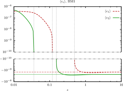
Figure 16: Averaged self-energy CP-violating parameters for Majorana neutrino and Higgs decay for benchmark point 1 as a function of the inverse temperature. Thin lines represent the value in the zero temperature limit. With conventional dispersion relations, the decay $N_{1}\rightarrow{\ell}\phi$ is active at $z>4.93\cdot 10^{-1}$ but replaced at high temperatures ($z<1.18\cdot 10^{-1}$) by $\bar{\phi}\rightarrow N_{1}{\ell}$. The decay $N_{2}\rightarrow{\ell}\phi$ is active at $z>1.54\cdot 10^{-1}$ but replaced at high temperatures ($z<3.62\cdot 10^{-2}$) by $\bar{\phi}\rightarrow N_{2}{\ell}$.

At very high temperatures the magnitude of $\langle\epsilon_{i}\rangle$ can be much larger for Higgs decay.

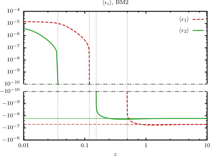
Figure 17: Averaged self-energy CP-violating parameters for Majorana neutrino and Higgs decay for benchmark point 2. See caption of Fig. 16.

As the temperature decreases the CP-violating parameter for the Higgs decay approaches zero. This is explained by the shrinking of the available phase space in the loop integrals (VII) and (VII).

VIII Conclusions

In this paper we have studied leptogenesis in the type-I seesaw extension of the Standard Model using the 2PI-formalism of non-equilibrium quantum field theory.

The asymmetry generation can, in the case of thermal leptogenesis, be approximately described by rate equations. Usually these statistical equations are treated as a ‘black-box’ in the sense that their form is assumed given and model specific amplitudes are inserted by hand. Indeed, this approach is supported by the observation that it describes the free decay in the zero temperature limit correctly and inherent inconsistencies (namely the ‘double-counting problem’) can be resolved in exact equilibrium. However, out of equilibrium it is not obvious whether the subtraction of real intermediate states works to all orders and how amplitudes computed in thermal field theory enter kinetic equations. These issues can be completely avoided in a systematic treatment within non-equilibrium quantum field theory.

Only in recent years fundamental questions related to the non-equilibrium statistical description received more attention. The progress here is mainly based on the 2PI-formalism which is known to yield consistent quantum kinetic equations without double-counting. These equations can be reduced to a system of Boltzmann-like kinetic equations for quasiparticles which can easily be compared to the conventional results. In the course of the derivation necessary approximations and the related physical assumptions have to be specified explicitly. Therefore, this approach enables a deeper insight into the dynamics of the asymmetry generation.

In the conventional analysis the minimal set of interactions is obtained at order $\mathcal{O}(h^{4})$ of the perturbative expansion. We have complemented existing analyses based on the 2PI-formalism by the computation of further processes which appear at this order. Starting from a system of Kadanoff-Baym and (equivalent) Schwinger-Dyson equations for leptons and heavy Majorana neutrinos we have derived Boltzmann-like quantum-kinetic equations for the lepton asymmetry. They include (inverse) decays of the heavy Majorana neutrinos as well as two-body scattering processes mediated by the heavy neutrinos:

$$\frac{s{\cal H}}{z}\frac{dY_{L}}{dz} =\sum_{i}\int{\,d\Pi_{{\ell}\phi N_{i}}^{pkq}}{\mathcal{F}_{{\ell}\phi\leftrightarrow N_{i}}^{pk;q}}\Xi_{{\ell}\phi\leftrightarrow N_{i}}$$

$$-\sum_{i}\int{\,d\Pi_{\bar{\ell}\bar{\phi}N_{i}}^{pkq}}{\mathcal{F}_{\bar{\ell}\bar{\phi}\leftrightarrow N_{i}}^{pk;q}}\Xi_{\bar{\ell}\bar{\phi}\leftrightarrow N_{i}}$$

$$-2\int{\,d\Pi_{{\ell}\phi\bar{\ell}\bar{\phi}}^{p_{1}k_{1}p_{2}k_{2}}}{\mathcal{F}_{\bar{\ell}\bar{\phi}\leftrightarrow{\ell}\phi}^{p_{2}k_{2};p_{1}k_{1}}}\Xi_{\bar{\ell}\bar{\phi}\leftrightarrow{\ell}\phi}$$

$$-\int{\,d\Pi_{{\ell}{\ell}\bar{\phi}\bar{\phi}}^{p_{1}p_{2}k_{1}k_{2}}}{\mathcal{F}_{\bar{\phi}\bar{\phi}\leftrightarrow{\ell}{\ell}}^{k_{1}k_{2};p_{1}p_{2}}}\Xi_{\bar{\phi}\bar{\phi}\leftrightarrow{\ell}{\ell}}$$

$$-\int{\,d\Pi_{\bar{\ell}\bar{\ell}\phi\phi}^{p_{1}p_{2}k_{1}k_{2}}}{\mathcal{F}_{\bar{\ell}\bar{\ell}\leftrightarrow\phi\phi}^{p_{1}p_{2};k_{1}k_{2}}}\Xi_{\bar{\ell}\bar{\ell}\leftrightarrow\phi\phi}{\,.}$$

Because all terms in this equation are proportional to $\cal F$, a combination of the distribution functions which vanishes in equilibrium, the obtained equations are free of the double-counting problem and no need for the real intermediate state subtraction arises. Together with the systematic derivation of the effective decay and scattering amplitudes $\Xi$ this is the main result of the present work. The individual amplitudes arise as combinations of different 2PI contributions. The vertex contribution to the CP-violating decay amplitude is obtained as cut of the 2PI ‘mercedes’ diagram. The same graph yields also the $s\times t$ contributions to ${\ell}\phi\leftrightarrow\bar{\ell}\bar{\phi}$ and the $u\times t$ contribution to ${\ell}{\ell}\leftrightarrow\bar{\phi}\bar{\phi}$ process. To extract the self-energy contribution, the off-diagonal elements of the Majorana neutrino propagator have to be taken into account. In addition, an extended quasiparticle approximation needs to be employed in order to obtain the $s\times s$ and $t\times t$ contributions to ${\ell}\phi\leftrightarrow\bar{\ell}\bar{\phi}$ as well as $u\times u$ and $t\times t$ contributions to ${\ell}{\ell}\leftrightarrow\bar{\phi}\bar{\phi}$ scattering from the ‘setting-sun’ diagram.

In the zero temperature limit the effective amplitudes reduce to the canonical ones. In particular, the form of the resulting amplitudes for ${\ell}\phi\leftrightarrow\bar{\ell}\bar{\phi}$ scattering coincides with the RIS subtracted amplitudes encountered in existing calculations. At finite temperatures the effective amplitudes receive thermal corrections. Medium corrections to the Majorana decay amplitudes into leptons and antileptons are $\mathcal{O}(h^{4})$. They are small compared to the tree-level vacuum contribution and are therefore negligible for the total decay width. On the other hand, they play an important role for the CP-violating source-terms, which are proportional to the difference of the two amplitudes. We find that medium corrections to the CP-violating parameter are linear in the particle number densities. Although there is a partial cancellation of the bosonic and fermionic contribution, the CP-violating parameter is enhanced. In the effective scattering amplitudes the medium corrections affect only the ‘regulator’ term in the denominator of the Breit-Wigner propagators. Due to the smallness of the Majorana decay width, which is constrained by the light neutrino masses, numerically these corrections are very small in the case of non-degenerate Majorana neutrinos.

Taking SM interactions into account in the form of thermal lepton and Higgs masses results in a suppression of the phase space for the Majorana neutrino decay and the enhancement of the CP-violating parameters is overcompensated. At even higher temperatures, when the effective Higgs mass exceeds the Majorana masses, the CP-violating decay of the Higgs into a lepton-Majorana pair can become kinematically allowed instead. At these temperatures the averaged CP-violating parameters for Higgs decay exceeds that obtained for Majorana decay in vacuum by orders of magnitude. The signs of the corresponding CP-violating parameters are opposite but their contribution to the lepton asymmetry has the same sign (at least in the limit of hierarchical Majorana masses). These results are in qualitative agreement with earlier studies based on thermal field theory and may ultimately be compared to a full treatment of CP-violating decays out of equilibrium, including gauge interactions.

We have also derived the corresponding rate equations for abundances of the participating species. They are obtained as expansion in small deviations from equilibrium ($\mu/T$ and $\Delta f_{N_{i}}$) and represent the hydrodynamical approximation of the Boltzmann kinetic equations. As compared to the standard (zero temperature) result they are improved in that the obtained coefficients include medium corrections to the quasiparticle properties and take into account quantum-statistical effects. We compare with the result obtained if the amplitudes are computed in thermal quantum field theory and the RIS subtraction is performed manually. We find that there are differences at higher order in the expansion parameters. The coefficients – reaction densities – reflect the interplay between the medium enhancement of the effective amplitudes and the phase space suppression induced by the thermal masses of Higgs and leptons. At very low temperatures the reaction densities approach their canonical limit.

Since for a hierarchical mass spectrum most of the asymmetry is typically generated by the lightest Majorana neutrino at temperatures of the order and smaller than its mass, we expect a moderate enhancement of the total generated asymmetry is possible for a typical average to strong washout scenario. For a detailed phenomenological analysis it is necessary to include further phenomena such as flavour effects and $\Delta L=1$ scattering processes which contribute to the washout at $\mathcal{O}(g^{2}h^{2})$. Additional quantum effects beyond the present analysis are relevant for non-standard scenarios in which the Majorana neutrinos have degenerate masses or if they are not as close to thermal equilibrium.

Acknowledgements

This work has been supported by the German Science Foundation (DFG) under Grant KA-3274/1-1 “Systematic analysis of baryogenesis in non-equilibrium quantum field theory” and the Collaborative Research Center 676 “Particles, Strings and the Early Universe”. T.F. acknowledges support by the IMPRS-PTFS. We thank S. Blanchet and M. Shaposhnikov for useful discussions.

Appendix A Kinematics

The reaction densities contain distribution functions of the initial and final states, which depend on the corresponding energies. Therefore to compute the reaction densities we need to analyze the kinematics of the decay and scattering processes.

A.1 Decay

To compute the CP-violating reaction density and the decay reaction density we need to evaluate the integral:

$$\langle X\gamma^{D}_{N_{i}}\rangle =\int\,d\Pi^{N}_{q}\,{f}_{N}^{eq}\int\,d\Pi^{\phi}_{k}\,d\Pi^{{\ell}}_{p}(2\pi)^{4}\delta(k+p-q)$$

$$\times X\Xi_{N}\bigl{[}1-{f}_{{\ell}}^{eq}+{f}_{\phi}^{eq}\bigr{]}{\,.}$$ (154)

For the washout reaction densities or reaction densities for Higgs decay we have similar expressions. The integration over $d^{3}k$ can be performed trivially and yields $\vec{k}=\vec{q}-\vec{p}$. Using $|\vec{k}|=(\vec{q}\,^{2}+\vec{p}\,^{2}-|\vec{q}||\vec{p}|\cos\theta)^{\frac{1}{2}}$ and integrating over $\theta$ we remove the remaining Dirac-delta and obtain

$$\int\,d\Pi^{\phi}_{p}\,d\Pi^{{\ell}}_{k}(2\pi)^{4} \delta(k+p-q) \rightarrow\frac{1}{8\pi\,|\vec{q}|}\int\limits_{E^{-}}^{E^{+}}dE_{p}\int\limits_{0}^{2\pi}\frac{d\varphi}{2\pi}{\,.}$$ (155)

The integration limits are given by

$$E^{\pm}={\textstyle\frac{1}{2}}\bigl{[}E_{q}\bigl{(}1+x_{\ell}-x_{\phi})\pm|\vec{q}|\lambda^{\frac{1}{2}}(1,x_{\ell},x_{\phi})\bigr{]}{\,,}$$ (156)

where $x_{\ell}\equiv m_{\ell}^{2}/q^{2}$, $x_{\phi}\equiv m_{\phi}^{2}/q^{2}$ and $\lambda(x,y,z)\equiv x^{2}+y^{2}+z^{2}-2xy-2xz-2yz$ is the usual kinematical function. For an on-shell heavy neutrino $q^{2}=M^{2}$. If $m_{\ell}=m_{\phi}=0$ then $\lambda(1,x_{\ell},x_{\phi})=1$ and the above expression simplifies to $E_{\pm}=\frac{1}{2}(E_{q}\pm|\vec{q}|)$. On the other hand, if $M=m_{\ell}+m_{\phi}$ then $\lambda(1,x_{\ell},x_{\phi})=0$ and therefore $E^{+}=E^{-}=E_{q}(m_{\ell}/M)$. Since the integration limits coincide in this case, the integral vanishes.

Combining it with the integration over $d^{3}q$ and using the isotropy of the medium we find

$$\langle X\gamma^{D}_{N_{i}}\rangle=\frac{1}{32\pi^{3}} \int\limits_{M}^{\infty}dE_{q}\,{f}_{N}^{eq}\int\limits_{E_{-}}^{E_{+}}dE_{p}X\Xi_{N}\bigl{[}1-{f}_{{\ell}}^{eq}+{f}_{\phi}^{eq}\bigr{]}{\,.}$$ (157)

If quantum-statistical effects are neglected then both the CP-violating parameter and the total tree-level decay amplitude are momentum independent and the integration can be performed analytically. We get:

$$\langle X\,\gamma^{D}_{N_{i}}\rangle\approx\frac{g_{N}}{2\pi^{2}}XM_{i}^{2}\Gamma_{i}TK_{1}\left(\frac{M_{i}}{T}\right){\,,}$$ (158)

where $g_{N}=2$ is the number of the Majorana spin degrees of freedom. Similar results are obtained for Higgs decay and washout reaction densities.

A.2 Two-body scattering

For $2\leftrightarrow 2$ scattering processes the reaction density is defined by

$$\langle\gamma^{ab}_{ij}\rangle \equiv\int{\,d\Pi_{abij}^{p_{a}p_{b}p_{i}p_{j}}}(2\pi)^{4}\delta(p_{a}+p_{b}-p_{i}-p_{j})$$

$$\times{f}_{a}^{eq}{f}_{b}^{eq}(1\pm{f}_{i}^{eq})(1\pm{f}_{j}^{eq})\Xi_{ab\leftrightarrow ij}{\,.}$$ (159)

To reduce it to a form suitable for the numerical analysis we insert an identity:

$$1=\int ds\int d^{4}q\delta(p_{a}+p_{b}-q)\delta_{+}(q^{2}-s){\,,}$$ (160)

into Eq. (A.2). The resulting expression can be interpreted as a product of the inverse decay and decay amplitudes integrated over the ‘mass’ and energy of the intermediate state:

$$\int{\,d\Pi_{abij}^{p_{a}p_{b}p_{i}p_{j}}} (2\pi)^{4}\delta(p_{a}+p_{b}-p_{i}-p_{j})$$

$$\rightarrow\int ds\int \frac{d^{4}q}{(2\pi)^{4}}\delta_{+}(q^{2}-s)$$

$$\times \int\,d\Pi^{a}_{p_{a}}\,d\Pi^{b}_{p_{b}}(2\pi)^{4}\delta(p_{a}+p_{b}-q)$$

$$\times \int\,d\Pi^{i}_{p_{i}}\,d\Pi^{j}_{p_{j}}(2\pi)^{4}\delta(q-p_{i}-p_{j}){\,.}$$ (161)

For the third line we will use Eq. (155). For the last line it is more convenient to us a different representation. Integrating out the delta-function we obtain for the last line in Eq. (A.2):

$$\frac{1}{4\pi}\int\frac{d\Omega_{i}}{4\pi}\frac{\vec{p}^{2}_{i}}{q_{0}|\vec{p}_{i}|-E_{i}|\vec{q}|\cos\Theta}{\,.}$$ (162)

Note that not all angles are kinematically allowed, see Eq. (A.2) below. As a product of Lorentz-invariant quantities the integral is also Lorentz-invariant. We can therefore boost to the center-of-mass frame where $\vec{q}=0$ and $q_{0}=\sqrt{s}$. By energy-momentum conservation $|\vec{p}_{i}|/q_{0}=\frac{1}{2}\lambda^{\frac{1}{2}}(1,x_{i},x_{j})$, where $q^{2}=s$ now. The angle integration can be partially reduced to integration over the Mandelstam variable $t=(p_{a}-p_{i})^{2}$ using the relation $dt=2|\vec{p}_{a}||\vec{p}_{i}|d\cos\theta_{ai}$. Note that the azimuthal angle $\varphi_{ai}$ is Lorentz-invariant by itself. Therefore, boosting back to the rest frame of the medium we can write the left-hand side of Eq. (162) in the form

$$\lambda^{-\frac{1}{2}}(1,x_{a},x_{b})\cdot\frac{1}{8\pi}\int\frac{d\varphi_{ai}}{2\pi}\int\frac{dt}{s}{\,.}$$ (163)

Integrating furthermore over $dq^{0}$ and using the fact the the integrand is independent of the orientation of $\vec{q}$, we finally obtain

$$\langle\gamma^{ab}_{ij}\rangle =\frac{1}{64\pi^{4}}\int\limits_{s_{min}}^{\infty}ds\int\limits_{\sqrt{s}}^{\infty}dE_{q}$$ (164)

$$\times\lambda^{-\frac{1}{2}}(1,x_{a},x_{b})\int\limits_{E^{-}}^{E^{+}}dE_{a}\,f^{eq}_{a}f^{eq}_{b}$$

$$\times\frac{1}{8\pi}\int\limits_{0}^{2\pi}\frac{d\varphi_{ai}}{2\pi}\int\limits_{t^{-}}^{t^{+}}\frac{dt}{s}\Xi_{ab\leftrightarrow ij}(1\pm{f}_{i}^{eq})(1\pm{f}_{j}^{eq}){\,,}$$

where $\sqrt{s}_{min}=\max(\sum m_{init},\sum m_{fin})$. Just like for particle decay, the integration limits $E^{\pm}$ are given by Eq. (156) but with $x_{\ell}$ and $x_{\phi}$ replaced by $x_{a}$ and $x_{b}$ respectively and the three-momentum given by $|\vec{q}|=(E_{q}^{2}-s)^{\frac{1}{2}}$. The range of integration over $t$ is given by

$$t^{\pm}=m_{a}^{2}+m_{i}^{2} -\frac{s}{2}\bigl{[}(1+x_{a}-x_{b})(1+x_{i}-x_{j})$$

$$\mp\lambda^{\frac{1}{2}}(1,x_{a},x_{b})\lambda^{\frac{1}{2}}(1,x_{i},x_{j})\bigr{]}{\,.}$$ (165)

In particular, for massless initial and finial states it reduces to $t^{+}=0$ and $t^{-}=-s$.

If the quantum-statistical effects are neglected then $f_{a}^{eq}(E_{a})f_{b}^{eq}(E_{b})=f_{N}^{eq}(E_{q})$. The integration over $E_{a}$ can be easily performed in this case and, combined with the $\lambda^{-\frac{1}{2}}(1,x_{a},x_{b})$ prefactor, gives $|\vec{q}|$. In the same approximation the last line of (164) does not depend on the distribution functions and gives so-called ‘reduced cross section’:

$$\hat{\sigma}(s)\equiv\frac{1}{8\pi}\int\limits_{0}^{2\pi}\frac{d\varphi_{ai}}{2\pi}\int\limits_{t^{-}}^{t^{+}}\frac{dt}{s}\Xi_{ab\leftrightarrow ij}{\,.}$$ (166)

Using Eq. (166) and integrating over $E_{q}$ we recover the usual expression for the scattering reaction density:

$$\langle\gamma^{ab}_{ij}\rangle \approx\frac{T}{64\pi^{4}}\int\limits_{s_{min}}^{\infty}ds\sqrt{s}K_{1}\left(\frac{\sqrt{s}}{T}\right)\hat{\sigma}(s){\,.}$$ (167)

To take the quantum-statistical effects into account we need to express energies of initial and final states in terms of the integration variables. By energy conservation $E_{b}=E_{q}-E_{a}$. Therefore $E_{a}$ and $E_{b}$ as well as the related momenta $|\vec{p}_{a}|$ and $|\vec{p}_{b}|$ are completely fixed by the second and third integration variables. Next we consider the final states. By energy conservation $E_{j}=E_{q}-E_{i}$. It remains to express $E_{i}$ in terms of the integration variables. Let us choose the coordinates such that $\vec{p}_{a}$ points along the $x$-axis and $\vec{p}_{b}$ lies in the $xy$-plane. Then the momentum transfer $\vec{q}$ also lies in the same plane. Its components are given by $\vec{q}=|\vec{q}|(\cos\theta_{aq},\sin\theta_{aq},0)$ where:

$$\cos\theta_{aq}=\frac{2E_{a}E_{q}-s+m_{b}^{2}-m_{a}^{2}}{2|\vec{q}||\vec{p}_{a}|}{\,.}$$ (168)

The components of $\vec{p}_{i}$ can be written in the form $\vec{p}_{i}=|\vec{p}_{i}|(\cos\theta_{ai},\sin\theta_{ai}\cos\varphi_{ai},\sin\theta_{ai}\sin\varphi_{ai})$. Then the angle between the vectors $\vec{p}_{i}$ and $\vec{q}$ is given by

$$\cos\theta_{qi} =\cos\theta_{aq}\cos\theta_{ai}+\sin\theta_{aq}\sin\theta_{ai}\cos\varphi_{ai}{\,.}$$ (169)

Using energy-momentum conservation we can express $E_{i}$ in terms of this angle and the integration variables:

$$E_{i}=\frac{1}{2}\frac{s}{s+\vec{q}^{2}\sin^{2}\theta_{qi}}\left[E_{q}\bigl{(}1+x_{i}-x_{j})\right.$$

$$+|\vec{q}|\cos\theta_{qi}\bigl{(}\lambda(1,x_{i},x_{j})-4x_{i}\vec{q}^{2}/s\sin^{2}\theta_{qi}\bigr{)}^{\frac{1}{2}}\bigr{]}{\,.}$$ (170)

Note that for $4m_{\ell}^{2}\vec{q}^{2}>\lambda(s,m_{\ell}^{2},m_{\phi}^{2})$ the difference under the square root in Eq. (A.2) can become negative for some angles. This means that such scattering angles are forbidden kinematically and should not be integrated over.

Since Eq. (A.2) implicitly depends on $\theta_{ai}$ it is convenient to use this angle as an integration variable instead of $t$. The integration measure in Eq. (164) is then modified according to $dt\rightarrow 2|\vec{p}_{a}||\vec{p}_{i}|\sin\theta_{ai}\,d\theta_{ai}$.

To calculate the scattering amplitudes we need the three Mandelstam variables. $s$ is an integration variable. $t$ is given by

$$t=m_{a}^{2}+m_{i}^{2}-2E_{a}E_{i}+2|\vec{p}_{a}||\vec{p}_{i}|\cos\theta_{ai}{\,.}$$ (171)

The remaining one, $u$, can be inferred from the Mandelstam relation $s+t+u=\sum m^{2}$.

Appendix B Generalized optical theorem and thermal cutting rules

The generalized optical theorem is a consequence of the unitarity of the $S$-matrix and can be seen as a consistency condition for the amplitudes to ensure conservation of probability. It can also be seen as a consequence of the Cutkosky cutting rules Cutkosky (1960); Eden et al. (2002); Le Bellac (1992) for the computation of the discontinuities of Feynman diagrams. As such it can be applied to unstable particles at any given order of perturbation theory. We may write it as

$$-i\Big{[} {\mathcal{M}}_{{a}\rightarrow{b}}(\{k_{i}\},\{p_{i}\})-{\mathcal{M}}_{{b}\rightarrow{a}}^{*}(\{p_{i}\},\{k_{i}\})\Big{]}=$$

$$=\sum_{i}\left(\prod_{i_{l}}\int{\,d\Pi_{i_{l}}}\right)(2\pi)^{4}\delta(\sum_{j}k_{j}-\sum_{i_{l}}q_{i_{l}})$$

$$\times{\mathcal{M}}_{{a}\rightarrow{i}}(\{k_{i}\},\{q_{i_{l}}\}){\mathcal{M}}_{{b}\rightarrow{i}}^{*}(\{p_{i}\},\{q_{i_{l}}\}){\,.}$$ (172)

The amplitudes ${\mathcal{M}}_{{a}\rightarrow{b}}$ include all contributing diagrams (at a given order of perturbation theory) and the sum on the right-hand side is over all possible real intermediate states $i$ which contribute to ${\mathcal{M}}_{{a}\rightarrow{b}}$. The generalized optical theorem can be exploited to see explicitly why the RIS subtraction works.

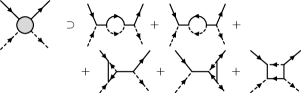
Figure 18: One-loop contributions to ${\ell}\phi\rightarrow{\ell}\phi$ scattering at $\mathcal{O}(h^{4})$. The cuts through the internal lepton and Higgs lines yield the $s\times s$, $s\times t$ and $t\times t$-contributions to ${\ell}\phi\rightarrow\bar{\ell}\bar{\phi}$. The cuts through single internal Majorana lines yield the interference terms which contribute to the CP-violating parameter.

To this end, we apply it to the forward scattering processes ${\ell}\phi\rightarrow{\ell}\phi$ and $\bar{{\ell}}\bar{\phi}\rightarrow\bar{{\ell}}\bar{\phi}$, see Fig. 18, above the energy thresholds $s>m_{N_{1}}^{2}$ (the contribution by $N_{2}$ real intermediate states etc. can be addressed analogously) and $s>(m_{{\ell}}+m_{\phi})^{2}$.

We include all possible graphs up to $\mathcal{O}(h^{4})$. Furthermore, we sum Eq. (172) over all internal degrees of freedom of initial and final states and absorb these in the ‘effective amplitudes’ defined in Sec. II. We get for the process involving particles

$$2\Im \big{\{}\sum_{\text{dof's}}{\mathcal{M}}_{{{\ell}\phi}\rightarrow{{\ell}\phi}}\big{\}}=\int{\,d\Pi^{N_{1}}_{q}}(2\pi)^{4}\delta(k+p-q)\Xi_{{\ell}\phi\rightarrow N_{1}}$$

$$+ \int{\,d\Pi^{{\ell}}_{q}\,d\Pi^{\phi}_{r}}(2\pi)^{4}\delta(k+p-q-r)\Xi_{{\ell}\phi\rightarrow\bar{{\ell}}\bar{\phi}}$$

$$+ \int{\,d\Pi^{{\ell}}_{q}\,d\Pi^{\phi}_{r}}(2\pi)^{4}\delta(k+p-q-r)\Xi_{{\ell}\phi\rightarrow{{\ell}}{\phi}}{\,.}$$ (173)

The amplitudes squared on the right-hand side contain the relevant graphs including the vertex and self-energy contributions, see Fig. 1, whose interference terms lead to CP-violation in the particle decay. In the same way one finds for $\bar{{\ell}}\bar{\phi}\leftrightarrow\bar{{\ell}}\bar{\phi}$:

$$2\Im \big{\{}\sum_{\text{dof's}}{\mathcal{M}}_{{\bar{{\ell}}\bar{\phi}}\rightarrow{\bar{{\ell}}\bar{\phi}}}\big{\}}=\int{\,d\Pi^{N_{1}}_{q}}(2\pi)^{4}\delta(k+p-q)\Xi_{\bar{{\ell}}\bar{\phi}\rightarrow N_{1}}$$

$$+ \int{\,d\Pi^{{\ell}}_{q}\,d\Pi^{\phi}_{r}}(2\pi)^{4}\delta(k+p-q-r)\Xi_{\bar{{\ell}}\bar{\phi}\rightarrow{\ell}\phi}$$

$$+ \int{\,d\Pi^{{\ell}}_{q}\,d\Pi^{\phi}_{r}}(2\pi)^{4}\delta(k+p-q-r)\Xi_{\bar{{\ell}}\bar{\phi}\rightarrow\bar{{\ell}}\bar{\phi}}{\,.}$$ (174)

As a consequence of CPT we have $\sum{\mathcal{M}}_{{{\ell}\phi}\rightarrow{{\ell}\phi}}=\sum{\mathcal{M}}_{{\bar{{\ell}}\bar{\phi}}\rightarrow{\bar{{\ell}}\bar{\phi}}}$. Therefore the difference of the left-hand sides of Eqs. (173) and (174) as well as that of the third terms on the right-hand-sides vanish. Subtracting the right-hand sides we obtain

$$\int{\,d\Pi^{{\ell}}_{q}\,d\Pi^{\phi}_{r}}(2\pi)^{4}\delta(k+p-q-r)\big{[}\Xi_{{\ell}\phi\rightarrow\bar{{\ell}}\bar{\phi}}-\Xi_{\bar{{\ell}}\bar{\phi}\rightarrow{\ell}\phi}\big{]}=$$

$$-\int{\,d\Pi^{N_{1}}_{q}}(2\pi)^{4}\delta(k+p-q)\big{[}\Xi_{{\ell}\phi\rightarrow N_{1}}-\Xi_{\bar{{\ell}}\bar{\phi}\rightarrow N_{1}}\big{]},$$ (175)

as a requirement for a consistent approximation of the amplitudes compatible with unitarity and CPT. It is obvious that this cannot be satisfied if the scattering amplitudes are in tree-level approximation meanwhile the decay amplitudes violate CP. We show in Sec. III how Eq. (175) can be satisfied by replacing the two-body scattering amplitudes $\Xi\rightarrow\Xi^{\prime}$. The solution for $\Xi^{\prime}$ amounts to subtracting the real intermediate state contributions from $\Xi$. In order to obtain an equivalent result for the Higgs decay at high temperature (i.e. for $m_{\phi}>m_{{\ell}}+M_{i}$) we need to consider different processes since the amplitude $\left|\mathcal{M}\right|_{{\bar{\phi}}\rightarrow{{\ell}N_{i}}}$ cannot be obtained as cut of the graphs in Fig. 18. One could try to draw and to cut graphs for ${\ell}N_{i}\rightarrow{\ell}N_{i}$ scattering, but the obtained cuts are lepton number conserving and would drop out in the difference $Y_{L}=Y_{{\ell}}-Y_{\bar{{\ell}}}$. Instead the relevant contributions appear as ‘thermal cuts’ of the $t$-channel contributions to ${\ell}\bar{\phi}\rightarrow{\ell}\bar{\phi}$ depicted in Fig. 19.

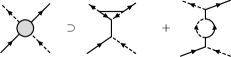
Figure 19: One-loop contributions to ${\ell}\bar{\phi}\rightarrow{\ell}\bar{\phi}$ scattering at $\mathcal{O}(h^{4})$. Due to medium effects the particles in the loop can be on-shell.

Since they exist only at finite density we need to use finite temperature ‘circling rules’, which can be seen as a generalization of Eq. (172), to compute the imaginary part of causal $n$-point functions in the real time formalism Kobes (1991):

$$2\Im\big{\{}i^{-1}\mathcal{F}_{R/A}^{(\alpha)}(x_{1},\ldots ,x_{\alpha},\ldots,x_{n};z_{j})\big{\}}=$$ (176)

$$\mp\sum_{x_{i}}^{\text{not all}}\sum_{z_{j}}\Im\Big{\{} i^{-1}F_{>}(x_{1},\ldots,\underline{x}_{\alpha},\ldots,x_{n};z_{j})-$$

$$- i^{-1}F_{<}(x_{1},\ldots,\underline{x}_{\alpha},\ldots,x_{n};z_{j})\Big{\}}{\,,}$$

where ‘not all’ means that not all $x_{i}$ should be circled at the same time. It was shown in Garny et al. (2010b) that causal $n$-point functions are the ones relevant for the computation of CP-violating parameters. The vertex $x_{\alpha}$ with largest or smallest time is always circled. We can use this equation together with the circling rules given in Kobes (1991); Garny et al. (2010b) to compute the imaginary parts of the graphs in Fig. 19 and the CPT-conjugated process $\bar{{\ell}}{\phi}\rightarrow\bar{{\ell}}{\phi}$. Taking the difference of both we obtain, similar to Eq. (175):

$$\int{\,d\Pi^{{\ell}}_{q}\,d\Pi^{\phi}_{r}}(2\pi)^{4}\delta(k+p-q-r)\big{[}\Xi_{{\ell}\phi\rightarrow\bar{{\ell}}\bar{\phi}}-\Xi_{\bar{{\ell}}\bar{\phi}\rightarrow{\ell}\phi}\big{]}=$$

$$-\int{\,d\Pi^{\phi}_{q}}(2\pi)^{4}\delta(k+p-q)\big{[}\Xi_{{\ell}N_{1}\rightarrow\bar{\phi}}-\Xi_{\bar{{\ell}N_{1}}\rightarrow\phi}\big{]}{\,.}$$ (177)

We can also use Eq. (176) to compute the thermal widths which cutoff the $s$- and $t$-channel resonances by cutting the self-energy graphs as shown in Fig. 20.

Figure 20: The thermal width can be obtained using (causal) finite temperature cutting rules.

Furthermore, the thermal CP-violating parameters can be obtained using thermal cutting rules, see e.g. Fig. 21

Figure 21: Circlings contributing to the self-energy (a),(b) and vertex (c-e) CP-violating parameter for Majorana neutrino decay and for Higgs decay (f),(g),(c-e). The contributions by graphs (b),(f) vanish since $N_{i}$ and $N_{j}$ cannot be on-shell simultaneously for $i\not=j$. Contributions by graphs (c-e) are suppressed if the cut is through an internal Majorana neutrino line.

and Garny et al. (2010b). Altogether, the concept of RIS subtraction can be generalized to include quantum-statistical effects using thermal quantum field theory in the real time formalism and a complete set of reaction densities can be computed. Note however that inconsistencies are inherent out of equilibrium and arise e.g. at higher order in the expansion performed in Sec. IV. Similar computations where performed in Kießig et al. (2010a); Kießig and Plümacher (2012a) in the imaginary time formalism of thermal quantum field theory.

Appendix C Rate equations

In this appendix we present some detailed intermediate steps in the derivation of rate equations with quantum-statistical terms. To obtain these we need to assume that the system is close to thermal equilibrium. Under certain conditions it is then possible to reduce Boltzmann-like equations to a set of rate equations for the systems evolution. Assuming that the detailed conditions given in Sec. IV are fulfilled and using Eq. (IV), we get for the integrated Boltzmann equations with quantum-statistical terms:

$$\int{\,d\Pi_{N_{i}{\ell}\phi}^{qpk}}\bigl{[}\pm\Xi_{N_{i}\rightleftarrows{\ell}\phi}{\mathcal{F}_{{\ell}\phi\leftrightarrow N_{i}}^{pk;q}}- \Xi_{N_{i}\rightleftarrows\bar{\ell}\bar{\phi}}{\mathcal{F}_{\bar{{\ell}}\bar{\phi}\leftrightarrow N_{i}}^{pk;q}}\bigr{]}$$ (178)

$$=\int{\,d\Pi_{N_{i}{\ell}\phi}^{qpk}}(2\pi)^{4}\,\delta(q-p-k)\Big{\{}\pm \Xi_{N_{i}\rightleftarrows{\ell}\phi}(1-f_{{\ell}})(1+f_{\phi})\big{[}\frac{f_{N_{i}}-{f}_{N_{i}}^{eq}}{(1-f_{N_{i}}){f}_{N_{i}}^{eq}}-(e^{+\frac{\mu_{{\ell}}+\mu_{\phi}}{T}}-1)\big{]}$$

$$- \Xi_{N_{i}\rightleftarrows\bar{\ell}\bar{\phi}}(1-f_{\bar{{\ell}}})(1+f_{\bar{\phi}})\big{[}\frac{f_{N_{i}}-{f}_{N_{i}}^{eq}}{(1-f_{N_{i}}){f}_{N_{i}}^{eq}}-(e^{-\frac{\mu_{{\ell}}+\mu_{\phi}}{T}}-1)\big{]}\Big{\}}(1-f_{N_{i}})\frac{{f}_{N_{i}}^{eq}}{(1-{f}_{N_{i}}^{eq})}{\,.}$$

This expression is still exact with respect to deviations from equilibrium and, taking into account results before Eq. (40), it has an obvious expansion in $\mu/T$. We can see that there will be contributions proportional to $\Delta f_{N_{i}}=({f_{N_{i}}-{f}_{N_{i}}^{eq}})$, to $\mu/T$ and proportional to $\Delta f_{N_{i}}\mu/T$ at linear order. The coefficients of these terms were introduced in Sec. IV (Eqs. (41) and (42)) and dubbed reaction densities. We find for the $\mathcal{O}(\mu/T)$ expansion of each of the two terms in Eq. (178), i.e. for the general collision term of $ab\leftrightarrow N$ in Eq. (IV):

$$\int{\,d\Pi_{Nab}^{qpk}}\Xi_{ab\leftrightarrow N}{\mathcal{F}_{ab\leftrightarrow N}^{pk;q}}\approx\bigg{<}\frac{\Xi_{ab\leftrightarrow N}}{\Xi_{N}}\frac{\Delta f_{N}}{{f}_{N}^{eq}}\gamma^{D}_{N}\bigg{>}$$

$$-\bigg{<}\frac{\Xi_{ab\leftrightarrow N}}{\Xi_{N}}\frac{\Delta f_{N}}{{f}_{N}^{eq}}(\xi_{a}\frac{a}{T}{f}_{a}^{eq}+\xi_{b}\frac{b}{T}{f}_{b}^{eq})\gamma^{D}_{N}\bigg{>}$$

$$-\frac{\mu_{a}+\mu_{b}}{T}\bigg{<}\frac{\Xi_{ab\leftrightarrow N}}{\Xi_{N}}\frac{(1-\xi^{N}f_{N})}{(1-\xi^{N}{f}_{N}^{eq})}\gamma^{W}_{N}\bigg{>}{\,,}$$ (179)

where we defined the decay reaction densities as

$$\langle X\gamma^{D}_{N}\rangle\equiv \int{\,d\Pi_{{a}{N}{b}}^{{p}{q}{k}}}\,(2\pi)^{4}\delta(q-k-p)X\Xi_{N}{f}_{N}^{eq}f_{ab}{\,,}$$

$$\langle X\gamma^{W}_{N}\rangle\equiv \big{<}X(1-{f}_{N}^{eq})\gamma^{D}_{N}\big{>}{\,,}$$ (180)

with $f_{ab}\equiv(1-\xi_{a}{f}_{a}^{eq}-\xi_{b}{f}_{b}^{eq})$. For a general process $aN\leftrightarrow b$ (where we allow again for deviations from equilibrium in $f_{N}$) we find in the same way:

$$\int{\,d\Pi_{Nab}^{qpk}}\Xi_{aN\leftrightarrow b}{\mathcal{F}_{aN\leftrightarrow b}^{pk;q}}\approx\bigg{<}-\frac{\Xi_{aN\leftrightarrow b}}{\Xi_{b}}\frac{\Delta f_{N}}{{f}_{N}^{eq}}\gamma^{D}_{b}\bigg{>}$$

$$-\bigg{<}\frac{\Xi_{aN\leftrightarrow b}}{\Xi_{b}}\frac{\Delta f_{N}}{{f}_{N}^{eq}}(-\frac{\mu_{a}}{T}(1-\xi_{a}{f}_{a}^{eq})+\xi_{b}\frac{\mu_{b}}{T}{f}_{b}^{eq})\gamma^{D}_{b}\bigg{>}$$

$$-\frac{\mu_{a}-\mu_{b}}{T}\bigg{<}\frac{\Xi_{aN\leftrightarrow b}}{\Xi_{b}}\frac{(1-\xi^{N}f_{N})}{(1-\xi^{N}{f}_{N}^{eq})}\gamma^{W}_{b}\bigg{>}{\,,}$$ (181)

where

$$\langle X\gamma^{D}_{b}\rangle\equiv \int{\,d\Pi_{{a}{N}{b}}^{{p}{q}{k}}}\,(2\pi)^{4}\delta(p+q-k)X\Xi_{b}{f}_{N}^{eq}f_{ab}{\,,}$$

$$\langle X\gamma^{W}_{b}\rangle\equiv \big{<}X(1-{f}_{N}^{eq})\gamma^{D}_{N}\big{>}{\,,}$$ (182)

with, now, $f_{ab}\equiv({f}_{a}^{eq}+\xi_{N}{f}_{b}^{eq})$. Note that these reaction densities will tend to zero in the zero temperature limit because of their dependence on the distribution functions. Using the general result (C) we obtain the contributions to Eq. (178), and therefore to Eq. (32), proportional to $\Delta f_{N_{i}}$,

$$\frac{s{\cal H}}{z}\frac{dY_{Li\atop N_{i}}}{dz}\Big{|}_{\Delta f_{N_{i}}}=\bigg{<}\frac{\pm\Xi_{N_{i}\rightleftarrows{\ell}\phi}-\Xi_{N_{i}\rightleftarrows\bar{{\ell}}\bar{\phi}}}{\Xi_{N_{i}}}\frac{\Delta f_{N_{i}}}{{f}_{N_{i}}^{eq}}\gamma^{D}_{N_{i}}\bigg{>}{\,,}$$ (183)

contributions proportional to $\Delta f_{N_{i}}\cdot{\frac{\mu_{\ell}}{T}}$,

$$\frac{s{\cal H}}{z}\frac{dY_{Li\atop N_{i}}}{dz}\Big{|}_{\Delta f_{N_{i}}{\frac{\mu_{\ell}}{T}}}=$$ (184)

$$\frac{\mu_{\ell}}{T}\bigg{<}\frac{\pm\Xi_{N_{i}\rightleftarrows{\ell}\phi}+\Xi_{N_{i}\rightleftarrows\bar{{\ell}}\bar{\phi}}}{{\Xi_{N_{i}}}}(c_{\phi{\ell}}{f}_{\phi}^{eq}-{f}_{{\ell}}^{eq})\frac{\Delta f_{N_{i}}}{{f}_{N_{i}}^{eq}}\gamma^{D}_{N_{i}}\bigg{>}$$

or just proportional to $\mu_{\ell}/T$:

$$\frac{s{\cal H}}{z}\frac{dY_{Li\atop N_{i}}}{dz}\Big{|}_{\frac{\mu_{\ell}}{T}}=$$ (185)

$$-\frac{\mu_{\ell}}{T}(1+c_{\phi{\ell}})\bigg{<}\frac{\pm\Xi_{N_{i}\rightleftarrows{\ell}\phi}+\Xi_{N_{i}\rightleftarrows\bar{{\ell}}\bar{\phi}}}{{\Xi_{N_{i}}}}\frac{(1-f_{N_{i}})}{(1-{f}_{N_{i}}^{eq})}\gamma^{W}_{N_{i}}\bigg{>}{\,.}$$

This leads immediately to the result in Eq. (44). Similarly, we get using Eq. (C) for the contributions (VII) by (anti-)Higgs decay to the rate equations:

$${\frac{s{\cal H}}{z}}\frac{dY_{Li\atop N_{i}}}{dz}\Big{|}_{\Delta f_{N_{i}}}=-\bigg{<}\frac{\Xi_{\bar{\phi}\rightarrow{\ell}N_{i}}\mp\Xi_{\phi\rightarrow\bar{{\ell}}N_{i}}}{\Xi_{\phi}}\frac{\Delta f_{N_{i}}}{{f}_{N_{i}}^{eq}}\gamma^{D}_{\phi}\bigg{>}{\,,}$$

$${\frac{s{\cal H}}{z}}\frac{dY_{Li\atop N_{i}}}{dz}\Big{|}_{\Delta f_{N_{i}}{\frac{\mu_{\ell}}{T}}}=$$

$$-\frac{\mu_{\ell}}{T}\bigg{<}\frac{\Xi_{\bar{\phi}\rightarrow{\ell}N_{i}}\mp\Xi_{\phi\rightarrow\bar{{\ell}}N_{i}}}{{\Xi_{\phi}}}(c_{\phi{\ell}}{f}_{\phi}^{eq}-(1-{f}_{{\ell}}^{eq}))\frac{\Delta f_{N_{i}}}{{f}_{N_{i}}^{eq}}\gamma^{D}_{\phi}\bigg{>}{\,,}$$

$${\frac{s{\cal H}}{z}}\frac{dY_{Li\atop N_{i}}}{dz}\Big{|}_{\frac{\mu_{\ell}}{T}}=$$

$$-\frac{\mu_{\ell}}{T}(1+c_{\phi{\ell}})\bigg{<}\frac{\Xi_{\bar{\phi}\rightarrow{\ell}N_{i}}\pm\Xi_{\phi\rightarrow\bar{\ell}N_{i}}}{{\Xi_{\phi}}}\frac{(1-f_{N_{i}})}{(1-{f}_{N_{i}}^{eq})}\gamma^{W}_{\phi}\bigg{>}{\,.}$$ (186)

In addition we get for the ’extra’ terms in Eqs. (33) and (IV):

$$\frac{dY_{Li\atop N_{i}}}{dz}\Big{|}_{D,\text{extra}} \propto(1\pm 1)\bigg{<}\frac{\Xi_{N_{i}\rightleftarrows{\ell}\phi}-\Xi_{{\ell}\phi\rightleftarrows N_{i}}}{{\Xi_{N_{i}}}}(1-f_{N_{i}})\gamma^{D}_{N_{i}}\bigg{>}+(1\mp 1)\frac{\mu_{\ell}}{T}(1+c_{\phi{\ell}})\bigg{<}\frac{\Xi_{N_{i}\rightleftarrows{\ell}\phi}-\Xi_{{\ell}\phi\rightleftarrows N_{i}}}{{\Xi_{N_{i}}}}(1-f_{N_{i}})\gamma^{D}_{N_{i}}\bigg{>}$$

$$+(1\mp 1)\frac{\mu_{\ell}}{T}\bigg{<}\frac{\Xi_{N_{i}\rightleftarrows{\ell}\phi}-\Xi_{{\ell}\phi\rightleftarrows N_{i}}}{{\Xi_{N_{i}}}}(c_{\phi{\ell}}{f}_{\phi}^{eq}-{f}_{{\ell}}^{eq})(1-f_{N_{i}})\gamma^{D}_{N_{i}}\bigg{>}{\,.}$$ (187)

This means that for ${dY_{Li}}/{dz}$ only the first term and for ${dY_{N_{i}}}/{dz}$ the last two terms contribute. The terms proportional to the difference of $\Xi_{N_{i}\rightleftarrows{\ell}\phi}$ and $\Xi_{N_{i}\rightleftarrows\bar{\ell}\bar{\phi}}$ lead to contributions proportional to the CP-violating parameter.

To reduce the two-body scattering terms in Eq. (35) we can use the same methods to find for the general expression,

$$\int {\,d\Pi_{abij}^{kpqr}}\,(2\pi)^{4}\delta(k+p-q-r)\Xi_{ab\leftrightarrow ij}$$ (188)

$$\times \big{[}(1-\xi^{a}f_{a})(1-\xi^{b}f_{b})f_{i}f_{j}\pm(1-\xi^{i}f_{i})(1-\xi^{j}f_{j})f_{a}f_{b}\big{]}{\,,}$$

the $\mathcal{O}(\mu/T)$ expansion:

$$\int{\,d\Pi_{abij}^{kpqr}}\,(2\pi)^{4}\delta(k+p-q-r)\Xi_{ab\leftrightarrow ij}$$

$$\times (1-\xi^{a}f_{a})(1-\xi^{b}f_{b})f_{i}f_{j}\big{[}(1\pm 1)\pm(e^{\frac{\mu_{a}+\mu_{b}-\mu_{i}-\mu_{j}}{T}}-1)\big{]}$$

$$= \frac{\mu_{c}+\mu_{d}\pm(\mu_{a}+\mu_{b})}{T}\langle\gamma^{ab}_{ij}\rangle+(1\pm 1)\langle\gamma^{ab}_{ij}\rangle$$

$$- (1\pm 1)\langle(\xi_{a}\frac{\mu_{a}}{T}{f}_{a}^{eq}+\xi_{b}\frac{\mu_{b}}{T}{f}_{b}^{eq}-\xi_{i}\frac{\mu_{i}}{T}{f}_{i}^{eq}-\xi_{j}\frac{\mu_{j}}{T}{f}_{j}^{eq})\gamma^{ab}_{ij}\rangle{\,,}$$

where the two-body scattering reaction density was introduced in Eq. (IV). The last expression results after first order expansion in $\mu/T$.

Appendix D 2PI effective action and self-energies

In this appendix we derive one-loop contribution to the self-energy of the Majorana field as well as one and two-loop contributions to the self-energy of leptons.

D.1 2PI effective action

The 2PI effective action is defined as a functional of the one- and two-point functions consisting of an infinite sum of all 2PI vacuum diagrams Cornwall et al. (1974). In practice, its expansion can be characterized in terms of the number of loops appearing in each diagram:

$$i\Gamma_{2\,\mathrm{PI}}[S,\mathscr{S},\Delta]=\sum_{n}i\Gamma_{2\,\mathrm{PI}}^{(n)}[S,\mathscr{S},\Delta]{\,.}$$ (189)

The two lowest order contributions, $i\Gamma_{2\,\mathrm{PI}}^{(2)}$ and $i\Gamma_{2\,\mathrm{PI}}^{(3)}$, relevant for leptogenesis are shown in Fig. 5. Their contributions to the 2PI action read

$$i\Gamma_{2\,\mathrm{PI}}^{(2)}= -\int_{\cal C}d^{4}u\ d^{4}w\ {\rm Tr}\big{[}hP_{R}\mathscr{S}(u,w)P_{L}\ h^{\dagger}$$

$$\hskip 60.0pt\ \times\ S(w,u)\epsilon\Delta^{*}(u,w)\epsilon\big{]}{\,,}\hphantom{aa}$$ (190a)

$$i\Gamma_{2\,\mathrm{PI}}^{(3)}= \frac{1}{2}\int_{\cal C}d^{4}u\ d^{4}w\ d^{4}\eta\ d^{4}\xi\ {\rm Tr}\big{[}hP_{R}\mathscr{S}(u,w)$$

$$\times CP_{R}h^{T}S^{T}(\eta,w)\epsilon\Delta^{*}(w,\xi)\epsilon h^{*}P_{L}C$$

$$\times\mathscr{S}(\eta,\xi)P_{L}h^{\dagger}S(\xi,u)\ \epsilon\Delta^{*}(u,\eta)\epsilon\big{]}{\,.}$$ (190b)

In Eq. (190) the trace is taken over flavor, Dirac and $SU(2)_{L}$ indices whereas the transposition only acts in flavor and Dirac space.

D.2 Lepton self-energies

By functional differentiation of the 2PI effective action with respect to the two-point function we obtain the corresponding self-energy which enters the Schwinger-Dyson equation:

$$\Sigma^{(n-1)}_{\alpha\beta}(x,y)=-i\frac{\delta\Gamma^{(n)}_{2\,\mathrm{PI}}[S]}{\delta S^{\,T}_{\beta\alpha}(y,x)}{\,.}$$ (191)

Here, flavor indices are shown explicitly whereas the $SU(2)_{L}$ and Dirac structure is embodied implicitly in matrix notation. The resulting self-energy is given by a combination of the Majorana, lepton and Higgs propagators. Since we do not consider the flavor effects and the early Universe was in an $SU(2)_{L}$-symmetric state:

$$\Delta_{ab}(x,y) =\delta_{ab}\Delta(x,y){\,,}\;\;S^{\alpha\beta}_{ab}(x,y)=\delta_{ab}\delta^{\alpha\beta}S(x,y){\,.}$$ (192a)

Since $\epsilon^{4}=-\epsilon^{2}=\mathbf{1}$ the lepton self-energy also becomes diagonal: $\Sigma^{\alpha\beta}_{ab}=\delta_{ab}\Sigma^{\alpha\beta}$. Furthermore, in the unflavored approximation it is convenient to sum over lepton flavors: $\Sigma\equiv\sum_{\alpha}\Sigma^{\alpha\alpha}$. Then the one- and two-loop order contributions to the lepton self-energy, see Fig. 5, take the form:

$$\Sigma^{(1)}(x,y)=-(h^{\dagger}h)_{ji}P_{R}\mathscr{S}^{ij}(x,y)P_{L}\Delta(y,x){\,,}$$ (193a)

$$\Sigma^{(2)}(x,y)=-(h^{\dagger}h)_{ij}(h^{\dagger}h)_{lk}\int_{\cal C}d^{4}wd^{4}\eta P_{R}\mathscr{S}^{jk}(x,w)C$$

$$\times P_{R}S^{T}(\eta,w)P_{L}C\mathscr{S}^{li}(\eta,y)P_{L}\Delta(y,w)\Delta(\eta,x){\,.}$$ (193b)

Eventually, it is the Wightman components that we are interested in since they enter the gain- and loss terms on the right-hand side of Eq. (69). Therefore, we insert the usual decomposition of the propagators $G\in\{\Delta,S,\mathscr{S}\}$ into the spectral and statistical parts, Eq. (61), into the self-energies (193a) and (193). A formal decomposition of the self-energy in analogy to (61) allows us to identify its spectral and statistical part and define the Wightman components in coordinate space as $\Sigma_{\gtrless}=\Sigma_{F}\mp\textstyle\frac{i}{2}\Sigma_{\rho}$. For the one-loop self-energy (193a) they read

$$\Sigma^{(1)}_{\gtrless}(x,y)=-(h^{\dagger}h)_{ji}P_{R}\mathscr{S}^{ij}_{\gtrless}(x,y)P_{L}\Delta_{\lessgtr}(y,x){\,.}$$ (194)

In the case of the two-loop contribution, Eq. (193), the computation becomes slightly elaborate. The complication is due to the appearance of 32 different terms after inserting the decomposition (61) for each of the five propagators into Eq. (193) as well as due to the two remaining integrations over the internal space-time arguments $w$ and $\eta$. The decomposition makes the path-ordering explicit and allows us to convert the integration along the CTP into an integration along the positive branch. The 32 terms contain different combinations of the $\mathrm{sign}$-functions. These can be rewritten by using relations given in Appendix C of Garny et al. (2009). After some simple but lengthy algebra we obtain for the Wightman components:

$$\Sigma^{(2)}_{\gtrless} (x,y)=(h^{\dagger}h)_{ij}(h^{\dagger}h)_{lk}\int d\omega\int d\eta$$

$$\times\bigl{[}P_{R}\mathscr{S}^{jk}_{R}(x,\omega)CP_{R}S^{T}_{F}(\eta,\omega)P_{L}C\mathscr{S}^{li}_{\gtrless}(\eta,y)P_{L}\ \Delta_{\lessgtr}(y,\omega)\Delta_{A}(\eta,x)$$

$$\;\,+P_{R}\mathscr{S}^{jk}_{F}(x,\omega)CP_{R}S^{T}_{R}(\eta,\omega)P_{L}C\mathscr{S}^{li}_{\gtrless}(\eta,y)P_{L}\ \Delta_{\lessgtr}(y,\omega)\Delta_{A}(\eta,x)$$

$$\;\,+P_{R}\mathscr{S}^{jk}_{R}(x,\omega)CP_{R}S^{T}_{A}(\eta,\omega)P_{L}C\mathscr{S}^{li}_{\gtrless}(\eta,y)P_{L}\ \Delta_{\lessgtr}(y,\omega)\Delta_{F}(\eta,x)$$

$$\;\,+P_{R}\mathscr{S}^{jk}_{\gtrless}(x,\omega)CP_{R}S^{T}_{R}(\eta,\omega)P_{L}C\mathscr{S}^{li}_{A}(\eta,y)P_{L}\ \Delta_{F}(y,\omega)\Delta_{\lessgtr}(\eta,x)$$

$$\;\,+P_{R}\mathscr{S}^{jk}_{\gtrless}(x,\omega)CP_{R}S^{T}_{A}(\eta,\omega)P_{L}C\mathscr{S}^{li}_{F}(\eta,y)P_{L}\ \Delta_{R}(y,\omega)\Delta_{\lessgtr}(\eta,x)$$

$$\;\,+P_{R}\mathscr{S}^{jk}_{\gtrless}(x,\omega)CP_{R}S^{T}_{F}(\eta,\omega)P_{L}C\mathscr{S}^{li}_{A}(\eta,y)P_{L}\ \Delta_{R}(y,\omega)\Delta_{\lessgtr}(\eta,x)$$

$$\;\,+P_{R}\mathscr{S}^{jk}_{R}(x,\omega)CP_{R}S^{T}_{\lessgtr}(\eta,\omega)P_{L}C\mathscr{S}^{li}_{A}(\eta,y)P_{L}\ \Delta_{\lessgtr}(y,\omega)\Delta_{\lessgtr}(\eta,x)$$

$$\;\,+P_{R}\mathscr{S}^{jk}_{\gtrless}(x,\omega)CP_{R}S^{T}_{\gtrless}(\eta,\omega)P_{L}C\mathscr{S}^{li}_{\gtrless}(\eta,y)P_{L}\ \Delta_{R}(y,\omega)\Delta_{A}(\eta,x)\bigr{]}{\,.}$$ (195)

Specific approximations will allow us to interpret both expressions, Eq. (194) and Eq. (D.2), as describing decay, inverse decay and scattering processes of quasiparticles in the medium.

The expressions for the one- and two-loop self-energies given by Eqs. (194) and (D.2) depend explicitly on two coordinates in four dimensional space-time. However, the self-energies which govern the gain- and loss term on the right-hand side of Eq. (69) are expressed in terms of phase space coordinates. Let us therefore exchange the pair of space-time arguments $(x,y)$ for an equivalent set of center and relative coordinates, $X\equiv(x+y)/2$ and $s\equiv x-y$. In contrast to thermal equilibrium, the out of equilibrium propagators depend not only on the relative coordinate $s$ but also on the center coordinate $X$. Performing a so-called Wigner transformation Calzetta and Hu (1988), i.e. a Fourier transformation with respect to the relative coordinate $s$, we can trade the latter for a momentum space variable:

$$G_{F}(X_{uv},p) =\int d^{4}s_{uv}e^{ips_{uv}}G_{F}(X_{uv},s_{uv}){\,,}$$ (196a)

$$G_{\rho}(X_{uv},p) =-i\int d^{4}s_{uv}e^{ips_{uv}}G_{\rho}(X_{uv},s_{uv}){\,,}\hphantom{aa}$$ (196b)

where we have used $X_{uv}=(u+v)/2$ and $s_{uv}=u-v$, $(u,v)\in\{x,y,w,\eta\}$ according to the various combinations appearing in Eqs. (194) and (D.2). Note that the factor $-i$ in the definition (196b) is conventional and makes the Wigner transform of the spectral propagator a hermitian matrix. Definitions of the Wigner transforms of the advanced and retarded propagators coincide with that for the statistical propagator.

The Wigner transform of Eq. (194) is obtained straightforwardly:

$$\Sigma^{(1)}_{\gtrless}(t,p)= -(h^{\dagger}h)_{ji}\int\,d\Pi^{4}_{k}\,d\Pi^{4}_{q}(2\pi)^{4}\delta(q-k-p)$$

$$\times P_{R}\mathscr{S}^{ij}_{\gtrless}(t,q)P_{L}\Delta_{\lessgtr}(t,k){\,.}$$ (197)

Note that motivated by the homogeneity and isotropy of the early Universe we only indicate time-dependence of the propagators and self-energy, $t\equiv X^{0}_{xy}$. To obtain the Wigner transform of Eq. (D.2) we will use an additional approximation: each of the Wigner transforms of the propagators we replace by $G(X_{uv},p)\rightarrow G(X,p)$. This means that we neglect the variations of $X_{uv}$ from the center coordinate $X=X_{xy}$ at which the self-energy is evaluated. Technically, it corresponds to a gradient expansion to lowest order and therefore disregards all memory effects. This can be compared to the ‘Stoßzahlansatz’ within the usual approach to the Boltzmann equation. It is convenient to represent the resulting expression as a sum of three terms:

$$\Sigma^{(2)}_{\gtrless}=\Sigma^{(2.1)}_{\gtrless}+\Sigma^{(2.2)}_{\gtrless}+\Sigma^{(2.3)}_{\gtrless}{\,.}$$ (198)

The first term on the right-hand side of Eq. (198) corresponds to the Wigner transform of lines one to three and four to six in Eq. (D.2):

$$\Sigma^{(2.1)}_{\gtrless}(t,p)=\int\,d\Pi^{4}_{q}\,d\Pi^{4}_{k}\ (2\pi)^{4}\delta(p-q+k)$$ (199)

$$\times\big{[}(h^{\dagger}h)_{ij}(h^{\dagger}h)_{lk}\varLambda_{jk}(t,q,k)P_{L}C\mathscr{S}^{li}_{\gtrless}(t,q)P_{L}\Delta_{\lessgtr}(t,k)$$

$$+(h^{\dagger}h)_{ji}(h^{\dagger}h)_{kl}P_{R}\mathscr{S}^{il}_{\gtrless}(t,q)CP_{R}V_{kj}(t,q,p)\Delta_{\lessgtr}(t,k)\big{]}{\,.}$$

where we have introduced two functions containing loop corrections:

$$\varLambda_{jk}(t,q,k)\equiv\int\,d\Pi^{4}_{k_{1}}\,d\Pi^{4}_{k_{2}}\,d\Pi^{4}_{k_{3}}$$

$$\times(2\pi)^{4}\delta(q+k_{1}+k_{2})\ (2\pi)^{4}\delta(k+k_{2}-k_{3})$$

$$\times\bigl{[}P_{R}\mathscr{S}^{jk}_{R}(t,-k_{3})CP_{R}S^{T}_{F}(t,k_{2})\Delta_{A}(t,k_{1})$$

$$+\ P_{R}\mathscr{S}^{jk}_{F}(t,-k_{3})CP_{R}S^{T}_{R}(t,k_{2})\Delta_{A}(t,k_{1})$$

$$+\ P_{R}\mathscr{S}^{jk}_{R}(t,-k_{3})CP_{R}S^{T}_{A}(t,k_{2})\Delta_{F}(t,k_{1})\bigr{]}{\,,}$$ (200)

and $V_{kj}(t,q,k)\equiv P\,\varLambda^{\dagger}_{kj}(t,q,k)\,P$. As we will see, (199) describes CP-violating decay of the heavy Majorana neutrino. The second term on the right-hand side of Eq. (198) is given by the Wigner transform of the seventh line of Eq. (D.2) and describes lepton number violating scattering processes:

$$\Sigma^{(2.2)}_{\gtrless}(t,p)=\int\,d\Pi^{4}_{p_{2}}\,d\Pi^{4}_{k_{1}}d\Pi_{k_{2}}(2\pi)^{4}\delta(p+k_{1}-p_{2}-k_{2})$$

$$\times(h^{\dagger}h)_{ij}(h^{\dagger}h)_{lk}\bigl{[}P_{R}\mathscr{S}^{jk}_{R}(t,p_{2}+k_{2})CP_{R}S^{T}_{\lessgtr}(t,-p_{2})P_{L}$$

$$\times C\mathscr{S}^{li}_{A}(t,p_{2}-k_{1})P_{L}\Delta_{\lessgtr}(t,k_{1})\Delta_{\lessgtr}(t,-k_{2})\bigr{]}{\,.}$$ (201)

Finally the last term in Eq. (198) corresponds to the last line of Eq. (D.2),

$$\Sigma^{(2.3)}_{\gtrless}(t,p)=\int d\Pi_{p_{2}}d\Pi_{k_{1}}d\Pi_{k_{2}}(2\pi)^{4}\delta(p+q_{1}-p_{2}-q_{2})$$

$$\times(h^{\dagger}h)_{ij}(h^{\dagger}h)_{lk}\bigl{[}P_{R}\mathscr{S}^{jk}_{\gtrless}(t,-q_{1})CP_{R}S^{T}_{\gtrless}(t,p_{2})P_{L}C$$

$$\times\mathscr{S}^{li}_{\gtrless}(t,q_{2})P_{L}\Delta_{A}(t,-q_{2}-p_{2})\Delta_{R}(t,q_{1}-p_{2})\bigr{]}{\,,}$$ (202)

and can be identified with lepton number conserving processes which do not contribute to generation of the lepton asymmetry.

D.3 Majorana self-energy

Differentiating Eq. (190) with respect to the two-point function of the Majorana neutrino and using definitions of the CP-conjugate two-point functions we obtain for the Majorana self-energy

$$\Pi^{ij}(x,y)= -g_{w}\bigl{[}(h^{\dagger}h)_{ij}\,P_{L}S(x,y)P_{R}\,\Delta(x,y)$$ (203)

$$+(h^{\dagger}h)^{*}_{ij}\,P_{R}P\bar{S}(\bar{x},\bar{y})PP_{L}\,\bar{\Delta}(\bar{x},\bar{y})\,\bigr{]}{\,,}$$

where we have assumed the $SU(2)_{L}$ symmetry of the medium and neglected flavor effects. The factor $g_{w}=2$ in Eq. (203) comes from the summation over the $SU(2)_{L}$ indices. The CP conjugate self-energy differs from Eq. (203) only in the propagators replaced by their CP conjugate counterparts and the couplings replaced by their complex conjugates.

From Eq. (203) we can read off the Wightman components of the self-energy:

$$\Pi^{ij}_{\gtrless}(x,y) =-g_{w}\bigl{[}(h^{\dagger}h)_{ij}P_{L}S_{\gtrless}(x,y)P_{R}\Delta_{\gtrless}(x,y)$$

$$+(h^{\dagger}h)^{*}_{ij}P_{R}P\bar{S}_{\gtrless}(\bar{x},\bar{y})\,PP_{L}\bar{\Delta}_{\gtrless}(\bar{x},\bar{y})\bigr{]}{\,.}$$ (204)

Its CP-conjugate can be obtained by complex conjugating the couplings and replacing the two-point functions by their CP-conjugates. To calculate amplitudes of the scattering processes we will need its Wigner transform:

$$\Pi^{ij}_{\gtrless}(t,q)= -g_{w}\int\,d\Pi^{4}_{k}\,d\Pi^{4}_{p}(2\pi)^{4}\delta(q-p-k)$$

$$\times\bigl{[}\,(h^{\dagger}h)_{ij}P_{L}S_{\gtrless}(t,p)P_{R}\Delta_{\gtrless}(t,p)$$

$$+(h^{\dagger}h)_{ji}P_{R}P\bar{S}_{\gtrless}(t,\bar{p})PP_{L}\bar{\Delta}_{\gtrless}(t,\bar{k})\bigr{]}{\,.}\hphantom{aaaa}$$ (205)

From Eq. (D.3) we can deduce the Wigner transform of the corresponding spectral self-energy:

$$\Pi^{ij}_{\rho}(t,q)= -{\frac{g_{w}}{16\pi}}\bigl{[}(h^{\dagger}h)_{ij}P_{L}\Pi_{\rho}(t,q)P_{R}$$

$$+(h^{\dagger}h)^{*}_{ij}P_{R}\bar{\Pi}_{\rho}(t,\bar{q})P_{L}\bigr{]}{\,,}$$ (206)

where we have introduced

$$\Pi_{\rho}(t,q) \equiv 16\pi{\textstyle\int}\,d\Pi^{4}_{k}\,d\Pi^{4}_{p}(2\pi)^{4}\delta(q-k-p)$$

$$\times\bigl{[}\Delta_{F}(t,k)S_{\rho}(t,p)+\Delta_{\rho}(t,k)S_{F}(t,p)\bigr{]}{\,,}$$

$$\Pi_{\rho}(t,q) \equiv 16\pi{\textstyle\int}\,d\Pi^{4}_{k}\,d\Pi^{4}_{p}(2\pi)^{4}\delta(q-k-p)$$

$$\times P\bigl{[}\bar{\Delta}_{F}(t,k)\bar{S}_{\rho}(t,p)+\bar{\Delta}_{\rho}(t,k)\bar{S}_{F}(t,p)\bigr{]}P{\,,}$$

and $\bar{q}\equiv(q^{0},-\vec{q}\,)$. In the quasiparticle approximation the Wigner transforms of the two-point functions of leptons and the Higgs are given by Eqs. (70)–(V.2) and Eqs. (79)–(80) respectively. In a CP-symmetric medium, which the early Universe was to a very good approximation, $\bar{\Delta}_{\rho}(t,k)=\Delta_{\rho}(t,k)$ and $\bar{\Delta}_{F}(t,k)=\Delta_{F}(t,k)$. The homogeneity and isotropy of the early Universe furthermore imply, that there is no dependence on the momentum direction and the spatial central coordinate so that $\bar{\Delta}_{\rho}(t,\bar{k})=\Delta_{\rho}(t,k)$ and $\bar{\Delta}_{F}(t,\bar{k})=\Delta_{F}(t,k)$. Just like for scalars, in a CP-symmetric medium the fermion two-point functions are related by $\bar{S}_{\rho}(t,p)=S_{\rho}(t,p)$ and $\bar{S}_{F}(t,p)=S_{F}(t,p)$. As for the $p\rightarrow\bar{p}$ transformation, the terms in the lepton propagators which carry spinor structure are not invariant under it:

$$P_{L}\,\not{\bar{p}}\,P_{R}=P_{L}P\,\not{p}\,PP_{R}=PP_{R}\,\not{p}\,P_{L}P{\,.}$$ (207)

Since $P^{2}=\mathbf{1}$, Eq. (207) implies that in a homogeneous, isotropic and CP-symmetric medium $\bar{\Pi}$ and $\Pi$ are left and right projections of the same ‘vector’ integral $L_{\rho}$:

$$\Pi^{ij}_{\rho} =-{\frac{g_{w}}{16\pi}}\bigl{[}(h^{\dagger}h)_{ij}P_{L}+(h^{\dagger}h)^{*}_{ij}P_{R}\,\bigr{]}L_{\rho}{\,.}$$ (208)

Explicit form of $L_{\rho}$ depends on the kinematic regime and is presented below.

To evaluate the decay amplitudes as well as amplitudes of the $s$-channel scattering processes we need to evaluate it for positive $q^{2}=M^{2}$ and $q^{2}=s$. If $q^{0}$ is also positive then $L_{\rho}$ takes the form:

$$L_{\rho}(t,q)=16\pi\int \,d\Pi^{\phi}_{k}\,d\Pi^{{\ell}}_{p}(2\pi)^{4}\delta(q-k-p)\,\not{p}$$

$$\times\,\bigl{[}1+f_{\phi}(t,k)-f_{\ell}(t,p)\bigr{]}{\,.}$$ (209)

To obtain Eq. (D.3) we have used the quasiparticle approximation for the two-point functions and integrated over the zeroth components of the momenta. Integrating out the energy-momentum conserving delta-function we obtain for its Lorentz components:

$$L^{0}_{\rho} =\frac{2T}{y}I_{1}\left(y_{0},y\right){\,,}$$ (210a)

$$\vec{L}_{\rho} =\frac{\vec{q}}{|\vec{q}|}\frac{2T}{y^{2}}\bigl{[}\,y_{0}I_{1}\left(y_{0},y\right)$$

$$-{\textstyle\frac{1}{2}}(y_{0}^{2}-y^{2})(1+x_{\ell}-x_{\phi})I_{0}\left(y_{0},y\right)\bigr{]}{\,,}$$ (210b)

where $y_{0}\equiv q^{0}/T$ and $y\equiv|\vec{q}|/T$. The integral functions $I_{n}$ are defined by

$$I_{n}(y_{0},y)\equiv\int\limits_{z^{-}}^{z^{+}}dz\,z^{n}\left(1+\frac{1}{e^{y_{0}-z}-1}-\frac{1}{e^{z}+1}\right){\,,}$$

where, in complete analogy with Eq. (156), the integration limits are given by

$$z^{\pm}={\textstyle\frac{1}{2}}\bigl{[}\,y_{0}\bigl{(}1+x_{\ell}-x_{\phi}\bigr{)}\pm y\lambda^{\frac{1}{2}}(1,x_{\ell},x_{\phi})\bigr{]}{\,.}$$ (211)

For positive $q^{2}$ and negative $q_{0}$ the components of $L_{\rho}$ are related to the ones above by $L^{0}_{\rho}(-q^{0},\vec{q}\,)=L^{0}_{\rho}(q^{0},\vec{q}\,)$ and $\vec{L}_{\rho}(-q^{0},\vec{q}\,)=-\vec{L}_{\rho}(q^{0},\vec{q}\,)$ respectively.

To evaluate amplitudes of the $t$- and $u$-channel processes we also need to calculate $L_{\rho}$ for negative square of the momentum transfer. In this case momentum-energy conservation ensures that $p^{0}$ and $k^{0}$ cannot be positive or negative simultaneously. If they have different signs then, assuming homogeneity and isotropy of the medium and using relations (124), we find

$$L_{\rho}(t,q) =16\pi{\textstyle\int}\,d\Pi^{\phi}_{k}\,d\Pi^{{\ell}}_{p}(2\pi)^{4}\,\not{p}$$

$$\times\bigl{\{} \delta(q+k-p)[f_{\bar{\phi}}(t,k)+f_{\ell}(t,p)]$$

$$+ \delta(q-k+p)[f_{\phi}(t,k)+f_{\bar{\ell}}(t,p)]\bigr{\}}{\,.}$$ (212)

Eq. (D.3) implies that for negative square of the momentum transfer $L_{\rho}$ vanishes in vacuum. Although it is in principle possible to retain the thermal masses of leptons and the Higgs in the calculation, the resulting expressions are quite lengthy in this case. Neglecting the thermal masses we obtain for the Lorentz components of $L_{\rho}$ in this regime:

$$L_{\rho}^{0} =\frac{2T}{y}\sum_{\pm}I_{1}^{\pm}(y_{0},y){\,,}$$ (213a)

$$\vec{L}_{\rho} =\frac{\vec{q}}{|\vec{q}|}\frac{2T}{y^{2}}\sum_{\pm}\bigl{[}\,y_{0}I_{1}^{\pm}(y_{0},y)-{\textstyle\frac{1}{2}}(y_{0}^{2}-y^{2})I_{0}^{\pm}(y_{0},y)\bigr{]}{\,,}$$ (213b)

where the integral functions are given by

$$I_{n}^{\pm}(y_{0},y)\equiv\int\limits_{\frac{1}{2}(y\pm y_{0})}^{\infty}dz\,z^{n}\left(\frac{1}{e^{z}+1}+\frac{1}{e^{z\mp y_{0}}-1}\right){\,.}$$

Note that in this regime $y>y_{0}$ and therefore the lower integration limit is positive.

To compute the scattering amplitude we need to calculate the product $qL_{\rho}$. For the $s$-channel we find:

$$qL_{\rho} =q^{2}(1+x_{\ell}-x_{\phi})\,y^{-1}I_{0}(y_{0},y){\,,}$$ (214)

whereas the corresponding expression for the $t$- and $u$-channels reads

$$qL_{\rho} =q^{2}\,y^{-1}\sum_{\pm}I_{0}^{\pm}(y_{0},y){\,.}$$ (215)

At low temperatures Eq. (215) is exponentially small and vanishes in the vacuum limit.

To analyze the Higgs decay we need to evaluate the spectral loop integral in a region of the phase space where the effective Higgs mass exceeds the sum of the Majorana and lepton masses. Using properties of the distribution functions under the $p^{0}\rightarrow-p^{0}$ transformation we find after some algebra from Eq. (VII):

$$L_{\rho}(t,q) =16\pi\int{\,d\Pi_{{\phi}{{\ell}}}^{{k}{p}}}(2\pi)^{4}\delta(q+p-k)\,\not{p}\bigl{[}\,{f}_{\phi}^{eq}+{f}_{{\ell}}^{eq}\,\bigr{]}.$$

Just like in Eq. (D.3), the integration is over the (on-shell) momenta of the Higgs and lepton and the Majorana momentum serves as a constraint. Note that in this case we are interested only in the on-shell Majorana momenta and therefore $q^{2}=M^{2}$. After integrating out the delta-function we obtain a result similar to Eq. (210):

$$L^{0}_{\rho} =\frac{2T}{y}J_{1}\left(y_{0},y\right){\,,}$$ (216)

$$\vec{L}_{\rho} =\frac{\vec{q}}{|\vec{q}|}\frac{2T}{y^{2}}\bigl{[}\,y_{0}J_{1}\left(y_{0},y\right)-{\textstyle\frac{1}{2}}(x_{\phi}-x_{\ell}-1)J_{0}\left(y_{0},y\right)\bigr{]}{\,,}$$ (217)

where the integral function is defined as:

$$J_{n}(y^{0},y)\equiv\int\limits^{z^{+}}_{z^{-}}dz\,z^{n}\left(\frac{1}{e^{z}+1}+\frac{1}{e^{z+y^{0}}-1}\right){\,.}$$

The integration limits are given by an expression similar to Eq. (211) but with $1+x_{\ell}-x_{\phi}$ replaced by $x_{\phi}-x_{\ell}-1$. When the effective Higgs mass approaches the kinematic limit, $m_{\phi}=m_{\ell}+M$ the upper integration limit approaches the lower one, and the integral vanishes.

Appendix E Numerical parameters

To perform the quantitative analysis we need to specify the Yukawa couplings. For simplicity we focus on the case of a very heavy third Majorana neutrino $M_{3}\gg M_{2}>M_{1}$ (MSM). In this limit the Yukawa couplings can be expressed in terms of the observed active neutrino masses and mixing angles and only one complex additional free parameter $\omega$.

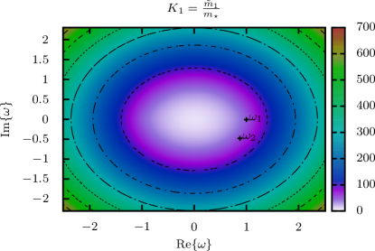
Figure 22: Washout parameter for $N_{1}$ decay in the complex $\omega$-plane. The values for the benchmark points are $K_{1}(\omega_{1})=47.20$ and $K_{1}(\omega_{2})=54.97$. $K_{1}$ has a minimum value of $K_{1}(0)=8.28$.

In the Casas-Ibarra parameterization Ibarra and Ross (2004); Antusch et al. (2012); Blanchet and Di Bari (2006); Guo et al. (2007) the Yukawa couplings are given by

$$(h^{\dagger}h)_{11} =\frac{M_{1}}{v^{2}}(m_{2}\left|1-\omega^{2}\right|+m_{3}\left|\omega^{2}\right|){\,,}$$ (218a)

$$(h^{\dagger}h)_{22} =\frac{M_{2}}{v^{2}}(m_{3}\left|1-\omega^{2}\right|+m_{2}\left|\omega^{2}\right|){\,,}$$ (218b)

$$(h^{\dagger}h)_{12} =\frac{\sqrt{M_{1}M_{2}}}{v^{2}}(m_{2}\,\omega\sqrt{1-\omega^{2}}\,^{*}-m_{3}\,\omega^{*}\sqrt{1-\omega^{2}}){\,,}$$ (218c)

where $v\approx 174$ GeV is the Higgs vev and we have assumed normal hierarchy. In this case the physical neutrino masses are given by

$$m_{2} =(\Delta m^{2}_{sol})^{\frac{1}{2}}\approx 8.71\cdot 10^{-12}\quad{\rm GeV}{\,,}$$

$$m_{3} =(\Delta m^{2}_{sol}+\Delta m^{2}_{atm})^{\frac{1}{2}}\approx 5.0\cdot 10^{-11}\quad{\rm GeV}{\,.}$$

For illustration we choose the benchmark points $\omega=\exp(-0.01\cdot I)$ and $\omega=\exp(-0.5\cdot I)$ denoted by BM1 and BM2 in the plots. As masses of the right-handed neutrinos we choose $M_{1}=10^{9}$ GeV and $M_{2}=\sqrt{10}M_{1}$ respectively. This choice of parameters is such that effects related to the resonant enhancement will be unimportant but contributions from both heavy Majorana neutrinos can be relevant. Note however that there are lower bounds on the washout parameters $K_{i}\equiv\Gamma_{i}/H\big{|}_{T=M_{1}}=\tilde{m}_{i}/m_{\star}$ (with ‘equilibrium neutrino mass’ $m_{\star}={16\pi^{5/2}\sqrt{g^{*}_{SM}}v^{2}/\big{(}3\sqrt{5}{M_{Pl}}\big{)}}$), see Figs. 22 and 23.

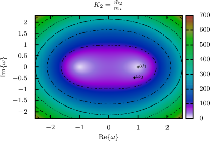
Figure 23: Washout parameter for $N_{2}$ decay in the complex $\omega$-plane. The values for the benchmark points are $K_{2}(\omega_{1})=9.22$ and $K_{2}(\omega_{2})=53.38$. $K_{2}$ has a minimum value of $K_{2}(-1)=K_{2}(1)=8.28173$.

The freeze-out of the asymmetry will therefore typically occur late (i.e. $T\ll M_{i}$) which renders medium effects in general small. However for the qualitative issues discussed in this paper our preference is to specify a consistent set of parameters for which we can discuss the generation of the lepton asymmetry in terms of two heavy Majorana neutrinos. This is of course not a general restriction for the employed techniques.

References

- ’t Hooft (1976) G. ’t Hooft, Phys. Rev. Lett. 37, 8 (1976).
- Klinkhamer and Manton (1984) F. R. Klinkhamer and N. Manton, Phys.Rev. D30, 2212 (1984).
- Kuzmin et al. (1985) V. A. Kuzmin, V. A. Rubakov, and M. E. Shaposhnikov, Phys. Lett. B 155, 36 (1985).
- Morrissey and Ramsey-Musolf (2012) D. E. Morrissey and M. J. Ramsey-Musolf (2012), eprint 1206.2942.
- Fukugita and Yanagida (1986) M. Fukugita and T. Yanagida, Phys. Lett. B 174, 45 (1986).
- Davidson and Ibarra (2002) S. Davidson and A. Ibarra, Phys. Lett. B 535, 25 (2002), eprint hep-ph/0202239.
- Hamaguchi et al. (2002) K. Hamaguchi, H. Murayama, and T. Yanagida, Phys.Rev. D65, 043512 (2002), eprint hep-ph/0109030.
- Sakharov (1967) A. D. Sakharov, JETP Letters 5, 24 (1967).
- Buchmüller et al. (2005a) W. Buchmüller, P. Di Bari, and M. Plümacher, Ann. Phys. 315, 305 (2005a), eprint hep-ph/0401240.
- Giudice et al. (2004) G. F. Giudice, A. Notari, M. Raidal, A. Riotto, and A. Strumia, Nucl. Phys. B 685, 89 (2004), eprint hep-ph/0310123.
- Davidson et al. (2008) S. Davidson, E. Nardi, and Y. Nir, Phys. Rept. 466, 105 (2008), eprint 0802.2962.
- Blanchet and Di Bari (2012) S. Blanchet and P. Di Bari (2012), eprint 1211.0512.
- Akhmedov et al. (1998) E. K. Akhmedov, V. Rubakov, and A. Y. Smirnov, Phys.Rev.Lett. 81, 1359 (1998), eprint hep-ph/9803255.
- Canetti et al. (2012) L. Canetti, M. Drewes, T. Frossard, and M. Shaposhnikov (2012), eprint 1208.4607.
- Garny et al. (2011) M. Garny, A. Kartavtsev, and A. Hohenegger (2011), eprint 1112.6428.
- Garbrecht and Herranen (2012) B. Garbrecht and M. Herranen, Nucl.Phys. B861, 17 (2012), eprint 1112.5954.
- Drewes and Garbrecht (2012) M. Drewes and B. Garbrecht (2012), eprint 1206.5537.
- Kolb and Turner (1990) E. W. Kolb and M. S. Turner, The Early universe (Addison-Wesley (Frontiers in physics, 69), Redwood City, CA, 1990).
- Buchmüller and Fredenhagen (2000) W. Buchmüller and S. Fredenhagen, Phys. Lett. B 483, 217 (2000), eprint hep-ph/0004145.
- Garny et al. (2009) M. Garny, A. Hohenegger, A. Kartavtsev, and M. Lindner, Phys. Rev. D 80, 125027 (2009), eprint 0909.1559.
- Garny et al. (2010a) M. Garny, A. Hohenegger, A. Kartavtsev, and M. Lindner, Phys. Rev. D 81, 085027 (2010a), eprint 0911.4122.
- Garny et al. (2010b) M. Garny, A. Hohenegger, and A. Kartavtsev, Phys. Rev. D 81, 085028 (2010b), eprint 1002.0331.
- Beneke et al. (2010) M. Beneke, B. Garbrecht, M. Herranen, and P. Schwaller, Nuclear Physics B 838, 1 (2010), eprint 1002.1326.
- Garny et al. (2010c) M. Garny, A. Hohenegger, and A. Kartavtsev (2010c), eprint 1005.5385.
- Garbrecht (2011) B. Garbrecht, Nucl.Phys. B847, 350 (2011), eprint 1011.3122.
- Anisimov et al. (2010a) A. Anisimov, W. Buchmüller, M. Drewes, and S. Mendizabal, Phys. Rev. Lett. 104, 121102 (2010a), eprint 1001.3856.
- Anisimov et al. (2010b) A. Anisimov, W. Buchmüller, M. Drewes, and S. Mendizabal (2010b), eprint 1012.5821.
- Beneke et al. (2011) M. Beneke, B. Garbrecht, C. Fidler, M. Herranen, and P. Schwaller, Nucl.Phys. B843, 177 (2011), eprint 1007.4783.
- Garbrecht (2012a) B. Garbrecht (2012a), eprint 1201.5126.
- Garbrecht (2012b) B. Garbrecht (2012b), eprint 1210.0553.
- Kießig and Plümacher (2012a) C. Kießig and M. Plümacher, JCAP 1207, 014 (2012a), eprint 1111.1231.
- Kießig and Plümacher (2012b) C. Kießig and M. Plümacher, JCAP 1209, 012 (2012b), eprint 1111.1235.
- Besak and Bodeker (2010) D. Besak and D. Bodeker, JHEP 1005, 007 (2010), eprint 1002.0022.
- Anisimov et al. (2011) A. Anisimov, D. Besak, and D. Bodeker, JCAP 1103, 042 (2011), eprint 1012.3784.
- Laine and Schroder (2012) M. Laine and Y. Schroder, JHEP 1202, 068 (2012), eprint 1112.1205.
- Salvio et al. (2011) A. Salvio, P. Lodone, and A. Strumia, JHEP 1108, 116 (2011), eprint 1106.2814.
- Besak and Bodeker (2012) D. Besak and D. Bodeker (2012), eprint 1202.1288.
- Flanz et al. (1995) M. Flanz, E. A. Paschos, and U. Sarkar, Phys. Lett. B 345, 248 (1995), erratum-ibid.B382:447,1996, eprint hep-ph/9411366.
- Covi et al. (1996) L. Covi, E. Roulet, and F. Vissani, Phys. Lett. B 384, 169 (1996), eprint hep-ph/9605319.
- Pilaftsis (1997) A. Pilaftsis, Phys. Rev. D 56, 5431 (1997).
- Pilaftsis and Underwood (2004) A. Pilaftsis and T. E. J. Underwood, Nucl. Phys. B 692, 303 (2004), eprint hep-ph/0309342.
- Plümacher (1998) M. Plümacher, Nucl. Phys. B 530, 207 (1998), eprint hep-ph/9704231.
- Kolb and Wolfram (1980) E. W. Kolb and S. Wolfram, Nucl. Phys. B 172, 224 (1980).
- Bernstein (1988) J. Bernstein, Kinetic Theory in the Expanding Universe (Cambridge University Press, Cambridge, 1988).
- Weinberg (1979) S. Weinberg, Phys. Rev. Lett. 42, 850–853 (1979).
- Roulet et al. (1998) E. Roulet, L. Covi, and F. Vissani, Phys. Lett. B 424, 101 (1998), eprint hep-ph/9712468.
- Kießig et al. (2010a) C. P. Kießig, M. Plümacher, and M. H. Thoma, Phys.Rev. D82, 036007 (2010a), eprint 1003.3016.
- Buchmüller et al. (2005b) W. Buchmüller, R. D. Peccei, and T. Yanagida, Ann. Rev. Nucl. Part. Sci. 55, 311 (2005b), eprint hep-ph/0502169.
- Kartavtsev (2006) A. Kartavtsev, Phys. Rev. D73, 023514 (2006), eprint hep-ph/0511059.
- Harvey and Turner (1990) J. A. Harvey and M. S. Turner, Phys. Rev. D 42, 3344 (1990).
- Basbøll and Hannestad (2007) A. Basbøll and S. Hannestad, JCAP 0701, 003 (2007), eprint hep-ph/0609025.
- Garayoa et al. (2009) J. Garayoa, S. Pastor, T. Pinto, N. Rius, and O. Vives, Journal of Cosmology and Astroparticle Physics 2009, 035 (2009), eprint 0905.4834.
- Hahn-Woernle et al. (2009) F. Hahn-Woernle, M. Plümacher, and Y. Y. Y. Wong, JCAP 0908, 028 (2009), eprint 0907.0205.
- Schwinger (1961) J. S. Schwinger, J. Math. Phys. 2, 407 (1961).
- Keldysh (1964) L. V. Keldysh, Zh. Eksp. Teor. Fiz. 47, 1515 (1964).
- Calzetta and Hu (1988) E. Calzetta and B. L. Hu, Phys. Rev. D 37, 2878 (1988).
- Berges (2004) J. Berges, AIP Conf. Proc. 739, 3 (2004), eprint hep-ph/0409233.
- Lindner and Müller (2006) M. Lindner and M. M. Müller, Phys. Rev. D 73, 125002 (2006), eprint hep-ph/0512147.
- De Simone and Riotto (2007) A. De Simone and A. Riotto, JCAP 0708, 002 (2007), eprint hep-ph/0703175.
- Lindner and Müller (2008) M. Lindner and M. M. Müller, Phys. Rev. D 77, 025027 (2008), eprint 0710.2917.
- Anisimov et al. (2009) A. Anisimov, W. Buchmüller, M. Drewes, and S. Mendizabal, Annals Phys. 324, 1234 (2009), eprint 0812.1934.
- Gagnon and Shaposhnikov (2011) J.-S. Gagnon and M. Shaposhnikov, Phys.Rev. D83, 065021 (2011), eprint 1012.1126.
- Drewes (2010) M. Drewes (2010), eprint 1012.5380.
- Cornwall et al. (1974) J. M. Cornwall, R. Jackiw, and E. Tomboulis, Phys. Rev. D 10, 2428 (1974).
- Hohenegger et al. (2008) A. Hohenegger, A. Kartavtsev, and M. Lindner, Phys. Rev. D 78, 085027 (2008), eprint 0807.4551.
- Toms (1987) D. J. Toms, Phys. Rev. D 35, 3796 (1987).
- Weldon (1989) H. A. Weldon, Physica A: Statistical and Theoretical Physics 158, 169 (1989).
- Kießig et al. (2010b) C. P. Kießig, M. Plümacher, and M. H. Thoma, Journal of Physics: Conference Series 259, 012079 (2010b).
- Carrington and Mrowczynski (2005) M. E. Carrington and S. Mrowczynski, Phys. Rev. D 71, 065007 (2005), eprint hep-ph/0406097.
- Spicka and Lipavsky (1994) V. Spicka and P. Lipavsky, Phys.Rev.Lett. 73, 3439 (1994).
- Spicka and Lipavsky (1995) V. Spicka and P. Lipavsky, Phys.Rev. B52, 14615 (1995).
- Morozov and Röpke (2006a) V. G. Morozov and G. Röpke, Cond. mat. Phys. 9, 473 (2006a).
- Köhler and Malfliet (1993) H. S. Köhler and R. Malfliet, Phys. Rev. C 48, 1034 (1993).
- Morozov and Röpke (2006b) V. G. Morozov and G. Röpke, Journal of Physics: Conference Series 35, 110 (2006b).
- Laine (2012) M. Laine (2012), eprint 1209.2869.
- Kajantie et al. (1996) K. Kajantie, M. Laine, K. Rummukainen, and M. Shaposhnikov, Nuclear Physics B 458, 90 – 136 (1996).
- Weldon (1982) H. A. Weldon, Phys.Rev. D26, 2789 (1982).
- Covi et al. (1998) L. Covi, N. Rius, E. Roulet, and F. Vissani, Phys. Rev. D 57, 93 (1998), eprint hep-ph/9704366.
- Cutkosky (1960) R. E. Cutkosky, Journal of Mathematical Physics 1, 429 (1960).
- Eden et al. (2002) R. J. Eden, P. V. Landshoff, D. I. Olive, and J. C. Polkinghorne, The Analytic S-Matrix (Cambridge University Press, 2002).
- Le Bellac (1992) M. Le Bellac, Quantum and Statistical Field Theory (Oxford University Press, 1992).
- Kobes (1991) R. L. Kobes, Phys. Rev. D 43, 1269 (1991).
- Ibarra and Ross (2004) A. Ibarra and G. G. Ross, Phys. Lett. B591, 285 (2004), eprint hep-ph/0312138.
- Antusch et al. (2012) S. Antusch, P. Di Bari, D. Jones, and S. King, Phys.Rev. D86, 023516 (2012), eprint 1107.6002.
- Blanchet and Di Bari (2006) S. Blanchet and P. Di Bari, JCAP 0606, 023 (2006), eprint hep-ph/0603107.
- Guo et al. (2007) W.-l. Guo, Z.-z. Xing, and S. Zhou, Int. J. Mod. Phys. E16, 1 (2007), eprint hep-ph/0612033.