Uniform convergence rates for nonparametric regression and principal component analysis in functional/longitudinal data

Abstract

We consider nonparametric estimation of the mean and covariance functions for functional/longitudinal data. Strong uniform convergence rates are developed for estimators that are local-linear smoothers. Our results are obtained in a unified framework in which the number of observations within each curve/cluster can be of any rate relative to the sample size. We show that the convergence rates for the procedures depend on both the number of sample curves and the number of observations on each curve. For sparse functional data, these rates are equivalent to the optimal rates in nonparametric regression. For dense functional data, root-$n$ rates of convergence can be achieved with proper choices of bandwidths. We further derive almost sure rates of convergence for principal component analysis using the estimated covariance function. The results are illustrated with simulation studies.

and

t1Supported by NSF Grant DMS-08-06131.

t2Supported by NSF Grants DMS-08-08993 and DMS-08-06098.

1 Introduction

Estimating the mean and covariance functions are essential problems in longitudinal and functional data analysis. Many recent papers focused on nonparametric estimation so as to model the mean and covariance structures flexibly. A partial list of such work includes Ramsay and Silverman (2005), Lin and Carroll (2000), Wang (2003), Yao, Müller and Wang (2005a, 2005b), Yao and Lee (2006) and Hall, Müller and Wang (2006).

On the other hand, functional principal component analysis (FPCA) based on nonparametric covariance estimation has become one of the most common dimension reduction approaches in functional data analysis. Applications include temporal trajectory interpolation [Yao, Müller and Wang (2005a)], functional generalized linear models [Müller and Stadtmüller (2005) and Yao, Müller and Wang (2005b)] and functional sliced inverse regression [Férre and Yao (2005), Li and Hsing (2010)], to name a few. A number of algorithms have been proposed for FPCA, some of which are based on spline smoothing [James, Hastie and Sugar (2000), Zhou, Huang and Carroll (2008)] and others based on kernel smoothing [Yao, Müller and Wang (2005a), Hall, Müller and Wang (2006)]. As usual, large-sample theories can provide a basis for understanding the properties of these estimators. So far, the asymptotic theories for estimators based on kernel smoothing or local-polynomial smoothing are better understood than those based on spline smoothing.

Some definitive theoretical findings on FPCA emerged in recent years. In particular, Hall and Hosseini-Nasab (2006) proved various asymptotic expansions for FPCA for densely recorded functional data, and Hall, Müller and Wang (2006) established the optimal $L^{2}$ convergence rate for FPCA in the sparse functional data setting. One of the most interesting findings in Hall, Müller and Wang (2006) was that the estimated eigenfunctions, although computed from an estimated two-dimensional surface, enjoy the convergence rate of one-dimensional smoothers, and under favorable conditions the estimated eigenvalues are root-$n$ consistent. In contrast with the $L^{2}$ convergence rates of these nonparametric estimators, less is known in term of uniform convergence rates. Yao, Müller and Wang (2005a) studied the uniform consistency of the estimated mean, covariance and eigenfunctions, and demonstrated that such uniform convergence properties are useful in many settings; some other examples can also be found in Li et al. (2008).

In classical nonparametric regression where observations are independent, there are a number of well-known results concerning the uniform convergence rates of kernel-based estimators. Those include Bickel and Rosenblatt (1973), Härdle, Janssen and Serfling (1988) and Härdle (1989). More recently, Claeskens and Van Keilegom (2003) extended some of those results to local likelihood estimators and local estimating equations. However, as remarked in Yao, Müller and Wang (2005a), whether those optimal rates can be extended to functional data remains unknown.

In a typical functional data setting, a sample of $n$ curves are observed at a set of discrete points; denote by $m_{i}$ the number of observations for curve $i$. The existing literature focuses on two antithetical data types: the first one, referred to as dense functional data, is the case where each $m_{i}$ is larger than some power of $n$; the second type, referred to as sparse functional data, is the situation where each $m_{i}$ is bounded by a finite positive number or follows a fixed distribution. The methodologies used to treat the two situations have been different in the literature. For dense functional data, the conventional approach is to smooth each individual curve first before further analysis; see Ramsay and Silverman (2005), Hall, Müller and Wang (2006) and Zhang and Chen (2007). For sparse functional data, limited information is given by the sparsely sampled observations from each individual curve and hence it is essential to pool the data in order to conduct inference effectively; see Yao, Müller and Wang (2005a) and Hall, Müller and Wang (2006). However, in practice it is possible that some sample curves are densely observed while others are sparsely observed. Moreover, in dealing with real data, it may even be difficult to classify which scenario we are faced with and hence to decide which methodology to use.

This paper is aimed at resolving the issues raised in the previous two paragraphs. The precise goals will be stated after we introduce the notation in Section 2. In a nutshell, we will consider uniform rates of convergence of the mean and the covariance functions, as well as rates in the ensuing FPCA, using local-linear smoothers [Fan and Gijbels (1995)]. The rates that we obtain will address all possible scenarios of the $m_{i}$’s, and we show that the optimal rates for dense and sparse functional data can be derived as special cases.

This paper is organized as follows. In Section 2, we introduce the model and data structure as well as all of the estimation procedures. We describe the asymptotic theory of the procedures in Section 3, where we also discuss the results and their connections to prominent results in the literature. Some simulation studies are provided in Section 4, and all proofs are included in Section 5.

2 Model and methodology

Let $\{X(t),t\in[a,b]\}$ be a stochastic process defined on a fixed interval $[a,b]$. Denote the mean and covariance function of the process by

$$\mu(t)=\mathbb{E}\{X(t)\},\qquad R(s,t)=\operatorname{cov}\{X(s),X(t)\},$$

which are assumed to exist. Except for smoothness conditions on $\mu$ and $R$, we do not impose any parametric structure on the distribution of $X$. This is a commonly considered situation in functional data analysis.

Suppose we observe

$$Y_{ij}=X_{i}(T_{ij})+U_{ij},\qquad i=1,\ldots,n,j=1,\ldots,m_{i},$$

where the $X_{i}$’s are independent realizations of $X$, the $T_{ij}$’s are random observational points with density function $f_{T}(\cdot)$, and the $U_{ij}$’s are identically distributed random errors with mean zero and finite variance $\sigma^{2}$. Assume that the $X_{i}$’s, $T_{ij}$’s and $U_{ij}$’s are all independent. Assume that $m_{i}\geq 2$ and let $N_{i}=m_{i}(m_{i}-1)$.

Our approach is based on the local-linear smoother; see, for example, Fan and Gijbels (1995). Let $K(\cdot)$ be a symmetric probability density function on $[0,1]$ and $K_{h}(t)=(1/h)K(t/h)$ where $h$ is bandwidth. A local-linear estimator of the mean function is given by $\widehat{\mu}(t)=\widehat{a}_{0}$, where

$$(\widehat{a}_{0},\widehat{a}_{1})=\mathop{\arg\min}_{a_{0},a_{1}}{1\over n}\sum_{i=1}^{n}{1\over m_{i}}\sum_{j=1}^{m_{i}}\{Y_{ij}-a_{0}-a_{1}(T_{ij}-t)\}^{2}K_{h_{\mu}}(T_{ij}-t).$$

It is easy to see that

$$\widehat{\mu}(t)={R_{0}S_{2}-R_{1}S_{1}\over S_{0}S_{2}-S_{1}^{2}},$$ (1)

where

$$S_{r} = {1\over n}\sum_{i=1}^{n}{1\over m_{i}}\sum_{j=1}^{m_{i}}K_{h_{\mu}}(T_{ij}-t)\{(T_{ij}-t)/h_{\mu}\}^{r},$$

$$R_{r} = {1\over n}\sum_{i=1}^{n}{1\over m_{i}}\sum_{j=1}^{m_{i}}K_{h_{\mu}}(T_{ij}-t)\{(T_{ij}-t)/h_{\mu}\}^{r}Y_{ij}.$$

To estimate $R(s,t)$, we first estimate $C(s,t):=\mathbb{E}\{X(s)X(t)\}$. Let $\widehat{C}(s,t)=\widehat{a}_{0}$, where

$$(\widehat{a}_{0},\widehat{a}_{1},\widehat{a}_{2})$$

$$\qquad=\mathop{\arg\min}_{a_{0},a_{1},a_{2}}{1\over n}\sum_{i=1}^{n}\biggl{[}{1\over N_{i}}\sum_{k\not=j}\{Y_{ij}Y_{ik}-a_{0}$$

(2)

$$\qquad\quad\hskip 96.31pt{}-a_{1}(T_{ij}-s)-a_{2}(T_{ik}-t)\}^{2}$$

$$\qquad\quad\hskip 100.39pt{}\times K_{h_{R}}(T_{ij}-s)K_{h_{R}}(T_{ik}-t)\biggr{]},$$

with $\sum_{k\not=j}$ denoting sum over all $k,j=1,\ldots,m_{i}$ such that $k\not=j$. It follows that

$$\widehat{C}(s,t)=(\mathcal{A}_{1}R_{00}-\mathcal{A}_{2}R_{10}-\mathcal{A}_{3}R_{01})\mathcal{B}^{-1},$$

where

$$\mathcal{A}_{1} = S_{20}S_{02}-S_{11}^{2},\qquad\mathcal{A}_{2}=S_{10}S_{02}-S_{01}S_{11},\qquad\mathcal{A}_{3}=S_{01}S_{20}-S_{10}S_{11},$$

$$\mathcal{B} = \mathcal{A}_{1}S_{00}-\mathcal{A}_{2}S_{10}-\mathcal{A}_{3}S_{01},$$

$$S_{pq} = {1\over n}\sum_{i=1}^{n}{1\over N_{i}}\sum_{k\not=j}\biggl{(}{T_{ij}-s\over h_{R}}\biggr{)}^{p}\biggl{(}{T_{ik}-t\over h_{R}}\biggr{)}^{q}K_{h_{R}}(T_{ij}-s)K_{h_{R}}(T_{ik}-t),$$

$$R_{pq} = {1\over n}\sum_{i=1}^{n}{1\over N_{i}}\sum_{k\not=j}Y_{ij}Y_{ik}\biggl{(}{T_{ij}-s\over h_{R}}\biggr{)}^{p}\biggl{(}{T_{ik}-t\over h_{R}}\biggr{)}^{q}K_{h_{R}}(T_{ij}-s)K_{h_{R}}(T_{ik}-t).$$

We then estimate $R(s,t)$ by

$$\widehat{R}(s,t)=\widehat{C}(s,t)-\widehat{\mu}(s)\widehat{\mu}(t).$$ (3)

To estimate $\sigma^{2}$, we first estimate $V(t):=C(t,t)+\sigma^{2}$ by $\widehat{V}(t)=\widehat{a}_{0}$, where

$$(\widehat{a}_{0},\widehat{a}_{1})=\mathop{\arg\min}_{a_{0},a_{1}}{1\over n}\sum_{i=1}^{n}{1\over m_{i}}\sum_{j=1}^{m_{i}}\{Y_{ij}^{2}-a_{0}-a_{1}(T_{ij}-t)\}^{2}K_{h_{V}}(T_{ij}-t).$$

As in (1),

$$\widehat{V}(t)={Q_{0}S_{2}-Q_{1}S_{1}\over S_{0}S_{2}-S_{1}^{2}},$$ (4)

where

$$Q_{r}={1\over n}\sum_{i=1}^{n}{1\over m_{i}}\sum_{j=1}^{m_{i}}K_{h_{V}}(T_{ij}-t)\{(T_{ij}-t)/h_{V}\}^{r}Y_{ij}^{2}.$$

We then estimate $\sigma^{2}$ by

$$\widehat{\sigma}^{2}={1\over b-a}\int_{a}^{b}\{\widehat{V}(t)-\widehat{C}(t,t)\}\,dt.$$

For the problem of mean and covariance estimation, the literature has focused on dense and sparse functional data. The sparse case roughly refers to the situation where each $m_{i}$ is essentially bounded by some finite number $M$. Yao, Müller and Wang (2005a) and Hall, Müller and Wang (2006) considered this case and also used local-linear smoothers in their estimation procedures. The difference between the estimators in (1), (3) and those considered in Yao, Müller and Wang (2005a) and Hall, Müller and Wang (2006) is essentially that we attach weights, $m_{i}^{-1}$ and $N_{i}^{-1}$, to each curve $i$ in the optimizations [although Yao, Müller and Wang (2005a) smoothed the residuals in estimating $R$]. One of the purposes of those weights is to ensure that the effect that each curve has on the optimizers is not overly affected by the denseness of the observations.

Dense functional data roughly refer to data for which each $m_{i}\geq M_{n}\to\infty$ for some sequence $M_{n}$, where specific assumptions on the rate of increase of $M_{n}$ are required for this case to have a distinguishable asymptotic theory in the estimation of the mean and covariance. Hall, Müller and Wang (2006) and Zhang and Chen (2007) considered the so-called “smooth-first-then-estimate” approach, namely, the approach that first preprocesses the discrete functional data by smoothing, and then adopts the empirical estimators of the mean and covariance based on the smoothed functional data. See also Ramsay and Silverman (2005).

As will be seen, our approach is suitable for both sparse and dense functional data. Thus, one particular advantage is that we do not have to discern data type—dense, sparse or mixed—and decide which methodology should be used accordingly. In Section 3, we will provide the convergence rates of $\widehat{\mu}(t),\widehat{R}(s,t)$ and $\widehat{\sigma}^{2}$, and also those of the estimated eigenvalues and eigenfunctions of the covariance operator of $X$. The novelties of our results include:

1. [(a)]

2. Almost-sure uniform rates of convergence for $\widehat{\mu}(t)$ and $\widehat{R}(s,t)$ over the entire range of $s,t$ will be proved.

3. The sample sizes $m_{i}$ per curve will be completely flexible. For the special cases of dense and sparse functional data, these rates match the best known/conjectured rates.

3 Asymptotic theory

To prove a general asymptotic theory, assume that $m_{i}$ may depend on $n$ as well, namely, $m_{i}=m_{in}$. However, for simplicity we continue to use the notation $m_{i}$. Define

$$\gamma_{nk}=\Biggl{(}n^{-1}\sum_{i=1}^{n}m_{i}^{-k}\Biggr{)}^{-1},\qquad k=1,2,\ldots,$$

which is the $k$th order harmonic mean of $\{m_{i}\}$, and for any bandwidth $h$,

$$\delta_{n1}(h)=[\{1+(h\gamma_{n1})^{-1}\}\log n/n]^{1/2}$$

and

$$\delta_{n2}(h)=[\{1+(h\gamma_{n1})^{-1}+(h^{2}\gamma_{n2})^{-1}\}\log n/n]^{1/2}.$$

We first state the assumptions. In the following $h_{\mu},h_{R}$ and $h_{V}$ are bandwidths, which are assumed to change with $n$.

1. [(C1)]

2. For some constants $m_{T}>0$ and $M_{T}<\infty$, $m_{T}\leq f_{T}(t)\leq M_{T}$ for all $t\in[a,b]$. Further, $f_{T}$ is differentiable with a bounded derivative.

3. The kernel function $K(\cdot)$ is a symmetric probability density function on $[-1,1]$, and is of bounded variation on $[-1,1]$. Denote $\nu_{2}=\int_{-1}^{1}t^{2}K(t)\,dt$.

4. $\mu(\cdot)$ is twice differentiable and the second derivative is bounded on $[a,b]$.

5. All second-order partial derivatives of $R(s,t)$ exist and are bounded on $[a,b]^{2}$.

6. $\mathbb{E}(|U_{ij}|^{\lambda_{\mu}})<\infty$ and $\mathbb{E}(\sup_{t\in[a,b]}|X(t)|^{\lambda_{\mu}})<\infty$ for some $\lambda_{\mu}\in(2,\infty)$; $h_{\mu}\to 0$ and $(h_{\mu}^{2}+h_{\mu}/\gamma_{n1})^{-1}(\log n/n)^{1-2/{\lambda_{\mu}}}\to 0$ as $n\to\infty$.

7. $\mathbb{E}(|U_{ij}|^{2\lambda_{R}})<\infty$ and $\mathbb{E}(\sup_{t\in[a,b]}|X(t)|^{2\lambda_{R}})<\infty$ for some $\lambda_{R}\in(2,\infty)$; $h_{R}\to 0$ and $(h_{R}^{4}+h_{R}^{3}/\gamma_{n1}+h_{R}^{2}/\gamma_{n2})^{-1}(\log n/n)^{1-2/\lambda_{R}}\to 0$ as $n\to\infty$.

8. $\mathbb{E}(|U_{ij}|^{2\lambda_{V}})<\infty$ and $\mathbb{E}(\sup_{t\in[a,b]}|X(t)|^{2\lambda_{V}})<\infty$ for some $\lambda_{V}\in(2,\infty)$; $h_{V}\to 0$ and $(h_{V}^{2}+h_{V}/\gamma_{n1})^{-1}(\log n/n)^{1-2/{\lambda_{V}}}\to 0$ as $n\to\infty$.

The moment condition $\mathbb{E}(\sup_{t\in[a,b]}|X(t)|^{\lambda})<\infty$ in (C5)–(C7) hold rather generally; in particular, it holds for Gaussian processes with continuous sample paths [cf. Landau and Shepp (1970)] for all $\lambda>0$. This condition was also adopted by Hall, Müller and Wang (2006).

3.1 Convergence rates in mean estimation

The convergence rate of $\widehat{\mu}(t)$ is given in the following result.

Theorem 3.1

Assume that (C1)–(C3) and (C5) hold. Then

$${\sup_{t\in[a,b]}}|\widehat{\mu}(t)-\mu(t)|=O\bigl{(}h_{\mu}^{2}+\delta_{n1}(h_{\mu})\bigr{)}\qquad\mbox{a.s.}$$ (5)

The following corollary addresses the special cases of sparse and dense functional data. For convenience, we use the notation $a_{n}\lesssim b_{n}$ to mean $a_{n}=O(b_{n})$.

Corollary 3.2

Assume that (C1)–(C3) and (C5) hold.

1. [(a)]

2. If $\max_{1\leq i\leq n}m_{i}\leq M$ for some fixed $M$, then

   $${\sup_{t\in[a,b]}}|\widehat{\mu}(t)-\mu(t)|=O\bigl{(}h_{\mu}^{2}+\{\log n/(nh_{\mu})\}^{1/2}\bigr{)}\qquad\mbox{a.s.}$$ (6)

3. If $\min_{1\leq i\leq n}m_{i}\geq M_{n}$ for some sequence $M_{n}$ where $M_{n}^{-1}\lesssim\break h_{\mu}\lesssim(\log n/n)^{1/4}$ is bounded away from $0$, then

   $${\sup_{t\in[a,b]}}|\widehat{\mu}(t)-\mu(t)|=O(\{\log n/n\}^{1/2})\qquad\mbox{a.s.}$$

The proofs of Theorem 3.1, as the proofs of other results, will be given in Section 5. First, we give a few remarks on these results.

Discussion

1. On the right-hand side of (5), $O(h_{\mu}^{2})$ is a bound for bias while $\delta_{n1}(h_{\mu})$ is a bound for ${\sup_{t\in[a,b]}}|\widehat{\mu}(t)-\mathbb{E}(\widehat{\mu}(t))|$. The derivation of the bias is easy to understand and is essentially the same as in classical nonparametric regression. The derivation of the second bound is more involved and represents our main contribution in this result. To obtain a uniform bound for $|\widehat{\mu}(t)-\mathbb{E}(\widehat{\mu}(t))|$ over $[a,b]$, we first obtained a uniform bound over a finite grid on $[a,b]$, where the grid grows increasingly dense with $n$, and then showed that the difference between the two uniform bounds is asymptotic negligible. This approach was inspired by Härdle, Janssen and Serfling (1988), which focused on nonparametric regression. One of the main difficulties in our result is that we need to deal within-curve dependence, which is not an issue in classical nonparametric regression. Note that the dependence between $X(t)$ and $X(t^{\prime})$ typically becomes stronger as $|t-t^{\prime}|$ becomes smaller. Thus, for dense functional data, the within-curve dependence constitutes an integral component of the overall rate derivation.

2. The sparse functional data setting in (a) of Corollary 3.2 was considered by Yao, Müller and Wang (2005a) and Hall, Müller and Wang (2006). Actually Yao, Müller and Wang (2005a) assumes that the $m_{i}$’s are i.i.d. positive random variables with $\mathbb{E}(m_{i})<\infty$, which implies that $0<1/\mathbb{E}(m_{i})\leq\mathbb{E}(1/m_{i})\leq 1$ by Jensen’s inequality; this corresponds to the case where $\gamma_{n1}$ is bounded away from 0 and also leads to (6). The rate in (6) is the classical nonparametric rate for estimating a univariate function. We will refer to this as a one-dimensional rate. The one-dimensional rate of $\widehat{\mu}(t)$ was eluded to in Yao, Müller and Wang (2005a) but was not specifically obtained there.

3. Hall, Müller and Wang (2006) and Zhang and Chen (2007) address the dense functional data setting in (b) of Corollary 3.2, where both papers take the approach of first fitting a smooth curve to $Y_{ij},1\leq j\leq m_{i}$, for each $i$, and then estimating $\mu(t)$ and $R(s,t)$ by the sample mean and covariance functions, respectively, of the fitted curves. Two drawbacks are:

   1. [(a)]

   2. Differentiability of the sample curves is required. Thus, for instance, this approach will not be suitable for the Brownian motion, which has continuous but nondifferentiable sample paths.

   3. The sample curves that are included in the analysis need to be all densely observed; those that do not meet the denseness criterion are dropped even though they may contain useful information.

   Our approach does not require sample-path differentiability and all of the data are used in the analysis. It is interesting to note that (b) of Corollary 3.2 shows that root-$n$ rate of convergence for $\widehat{\mu}$ can be achieved if the number of observations per sample curve is at least of the order $(n/\log n)^{1/4}$ while a similar conclusion was also reached in Hall, Müller and Wang (2006) for the smooth-first-then-estimate approach.

4. Our nonparametric estimators $\widehat{\mu}$, $\widehat{R}$ and $\widehat{V}$ are based local-linear smoothers, but the methodology and theory can be easily generalized to higher-order local-polynomial smoothers. By the equivalent kernel theory for local-polynomial smoothing [Fan and Gijbels (1995)], higher-order local-polynomial smoothing is asymptotically equivalent to higher-order kernel smothing. Therefore, applying higher-order polynomial smoothing will result in improved rates for the bias under suitable smoothness assumptions. The rate for the variance, on the other hand, will remain the same. In our sparse setting, if $p$th order local polynomial smoothing is applied under suitable conditions, for some positive integer $p$, the uniform convergence rate of $\widehat{\mu}(t)$ will become

   $${\sup_{t}}|\widehat{\mu}(t)-\mu(t)|=O\bigl{(}h_{\mu}^{2([p/2]+1)}+\delta_{n1}(h_{\mu})\bigr{)}\qquad\mbox{a.s.},$$

   where $[a]$ denotes the integer part of $a$. See Claeskens and Van Keilegom (2003) and Masry (1996) for support of this claim in different but related contexts.

3.2 Convergence rates in covariance estimation

The following results give the convergence rates for $\widehat{R}(s,t)$ and $\widehat{\sigma}^{2}$.

Theorem 3.3

Assume that (C1)–(C6) hold. Then

$${\sup_{s,t\in[a,b]}}|\widehat{R}(s,t)-R(s,t)|=O\bigl{(}h_{\mu}^{2}+\delta_{n1}(h_{\mu})+h_{R}^{2}+\delta_{n2}(h_{R})\bigr{)}\qquad\mbox{a.s.}$$ (7)

Theorem 3.4

Assume that (C1), (C2), (C4), (C6) and (C7) hold. Then

$$\widehat{\sigma}^{2}-\sigma^{2}=O\bigl{(}h_{R}^{2}+\delta_{n1}(h_{R})+\delta_{n2}^{2}(h_{R})+h_{V}^{2}+\delta_{n1}^{2}(h_{V})\bigr{)}\qquad\mbox{a.s.}$$ (8)

We again highlight the cases of sparse and dense functional data.

Corollary 3.5

Assume that (C1)–(C7) hold.

1. [(a)]

2. Suppose that $\max_{1\leq i\leq n}m_{i}\leq M$ for some fixed $M$. If $h_{R}^{2}\lesssim h_{\mu}\lesssim h_{R}$, then

   $${\sup_{s,t\in[a,b]}}|\widehat{R}(s,t)-R(s,t)|=O\bigl{(}h_{R}^{2}+\{\log n/(nh_{R}^{2})\}^{1/2}\bigr{)}\qquad\mbox{a.s.}$$ (9)

   If $h_{V}+(\log n/n)^{1/3}\lesssim h_{R}\lesssim h_{V}^{2}n/\log n$, then

   $$\widehat{\sigma}^{2}-\sigma^{2}=O\bigl{(}h_{R}^{2}+\{\log n/(nh_{R})\}^{1/2}\bigr{)}\qquad\mbox{a.s.}$$

3. If $\min_{1\leq i\leq n}m_{i}\geq M_{n}$ for some sequence $M_{n}$ where $M_{n}^{-1}\lesssim h_{\mu},h_{R},h_{V}\lesssim(\log n/n)^{1/4}$, then both ${\sup_{s,t\in[a,b]}}|\widehat{R}(s,t)-R(s,t)|$ and $\widehat{\sigma}^{2}-\sigma^{2}$ are$O(\{\log n/n\}^{1/2})$ a.s.

Discussion

1. The rate in (9) is the classical nonparametric rate for estimating a surface (bivariate function), which will be referred to as a two-dimensional rate. Note $\widehat{\sigma}^{2}$ has a one-dimensional rate in the sparse setting, while both $\widehat{R}(s,t)$ and $\widehat{\sigma}^{2}$ have root-$n$ rates in the dense setting. Most of the discussions in Section 3.1 obviously also apply here and will not be repeated.

2. Yao, Müller and Wang (2005a) smoothed the products of residuals instead of $Y_{ij}Y_{ik}$ in the local linear smoothing algorithm in (2). There is some evidence that a slightly better rate can be achieved in that procedure. However, we were not successful in establishing such a rate rigorously.

3.3 Convergence rates in FPCA

By (C5), the covariance function has the spectral decomposition

$$R(s,t)=\sum_{j=1}^{\infty}\omega_{j}\psi_{j}(s)\psi_{j}(t),$$

where $\omega_{1}\geq\omega_{2}\geq\cdots\geq 0$ are the eigenvalues of $R(\cdot,\cdot)$ and the $\psi_{j}$’s are the corresponding eigenfunctions. The $\psi_{j}$’s are also known as the functional principal components. Below, we assume that the nonzero $\omega_{j}$’s are distinct.

Suppose $\widehat{R}(s,t)$ is the covariance estimator given in Section 2, and it admits the following spectral decomposition:

$$\widehat{R}(s,t)=\sum_{j=1}^{\infty}\widehat{\omega}_{j}\widehat{\psi}_{j}(s)\widehat{\psi}_{j}(t),$$

where $\widehat{\omega}_{1}>\widehat{\omega}_{2}>\cdots$ are the estimated eigenvalues and the $\widehat{\psi}_{j}$’s are the corresponding estimated principal components. Computing the eigenvalues and eigenfunctions of an integral operator with a symmetric kernel is a well-studied problem in applied mathematics. We will not get into that aspect of FPCA in this paper.

Notice also that $\psi_{j}(t)$ and $\widehat{\psi}_{j}(t)$ are identifiable up to a sign change. As pointed out in Hall, Müller and Wang (2006), this causes no problem in practice, except when we discuss the convergence rate of $\widehat{\psi}_{j}$. Following the same convention as in Hall, Müller and Wang (2006), we let $\psi_{j}$ take an arbitrary sign but choose $\widehat{\psi}_{j}$ such that $\|\widehat{\psi}_{j}-\psi_{j}\|$ is minimized over the two signs, where $\|f\|:=\{\int f^{2}(t)\,dt\}^{1/2}$ denotes the usual $L^{2}$-norm of a function $f\in L^{2}[a,b]$.

Below let $j_{0}$ be a arbitrary fixed positive constant.

Theorem 3.6

Under conditions (C1)–(C6), for $1\leq j\leq j_{0}$:

1. [(a)]

2. $\widehat{\omega}_{j}-\omega_{j}=O((\log n/n)^{1/2}+h_{\mu}^{2}+h_{R}^{2}+\delta_{n1}^{2}(h_{\mu})+\delta_{n2}^{2}(h_{R}))$ a.s.;

3. $\|\widehat{\psi}_{j}-\psi_{j}\|=O(h_{\mu}^{2}+\delta_{n1}(h_{\mu})+h_{R}^{2}+\delta_{n1}(h_{R})+\delta_{n2}^{2}(h_{R}))$ a.s.;

4. ${\sup_{t}}|\widehat{\psi}_{j}(t)-\psi_{j}(t)|=O(h_{\mu}^{2}+\delta_{n1}(h_{\mu})+h_{R}^{2}+\delta_{n1}(h_{R})+\delta_{n2}^{2}(h_{R}))$ a.s.

Theorem 3.6 is proved by using the asymptotic expansions of eigenvalues and eigenfunctions of an estimated covariance function developed by Hall and Hosseini-Nasab (2006), and by applying the strong uniform convergence rate of $\widehat{R}(s,t)$ in Theorem 3.3. In the special case of sparse and dense functional data, we have the following corollary.

Corollary 3.7

Assume that (C1)–(C6) hold. Suppose that$\max_{1\leq i\leq n}m_{i}\leq M$ for some fixed $M$. Then the following hold for all $1\leq j\leq j_{0}$:

1. [(a)]

2. If $(\log n/n)^{1/2}\lesssim h_{\mu},h_{R}\lesssim(\log n/n)^{1/4}$ then $\widehat{\omega}_{j}-\omega_{j}=O(\{\log n/n\}^{1/2})$ a.s.

3. If $h_{\mu}+(\log n/n)^{1/3}\lesssim h_{R}\lesssim h_{\mu}$ then both of $\|\widehat{\psi}_{j}-\psi_{j}\|$ and ${\sup_{t}}|\widehat{\psi}_{j}(t)-\psi_{j}(t)|$ have the rate $O(h_{R}^{2}+\{\log n/(nh_{R})\}^{1/2})$ a.s.

If $\min_{1\leq i\leq n}m_{i}\geq M_{n}$ for some sequence $M_{n}$ where $M_{n}^{-1}\lesssim h_{\mu},h_{R}\lesssim(\log n/n)^{1/4}$, then, for $1\leq j\leq j_{0}$, all of $\widehat{\omega}_{j}-\omega_{j}$, $\|\widehat{\psi}_{j}-\psi_{j}\|$ and $\sup_{t}|\widehat{\psi}_{j}(t)-\psi_{j}(t)|$ have the rate $O(\{\log n/n\}^{1/2})$.

Discussion

1. Yao, Müller and Wang (2005a, 2005b) developed rate estimates for the quantities in Theorem 3.6. However, they are not optimal. Hall, Müller and Wang (2006) considered the rates of $\widehat{\omega}_{j}-\omega_{j}$ and $\|\widehat{\psi}_{j}-\psi_{j}\|$. The most striking insight of their results is that for sparse functional data, even though the estimated covariance operator has the two-dimensional nonparametric rate, $\widehat{\psi}_{j}$ converges at a one-dimensional rate while $\widehat{\omega}_{j}$ converges at a root-$n$ rate if suitable smoothing parameters are used; remarkably they also established the asymptotic distribution of $\|\widehat{\psi}_{j}-\psi_{j}\|$. At first sight, it may seem counter-intuitive that the convergence rates of $\widehat{\omega}_{j}$ and $\widehat{\psi}_{j}$ are faster than that of $\widehat{R}$, since $\widehat{\omega}_{j}$ and $\widehat{\psi}_{j}$ are computed from $\widehat{R}$. However, this can be easily explained. For example, by (4.9) of Hall, Müller and Wang (2006), $\widehat{\omega}_{j}-\omega_{j}=\int\!\!\int(\widehat{R}(s,t)-R(s,t))\psi_{j}(s)\psi_{j}(t)\,ds\,dt+\mathrm{lower}$-order terms; integrating $\widehat{R}(s,t)-R(s,t)$ in this expression results in extra smoothing, which leads to a faster convergence rate.

2. Our almost-sure convergence rates are new. However, for both dense and sparse functional data, the rates on $\widehat{\omega}_{j}-\omega_{j}$ and $\|\widehat{\psi}_{j}-\psi_{j}\|$ are slightly slower than the in-probability convergence rates obtained in Hall, Müller and Wang (2006), which do not contain the $\log n$ factor at various places of our rate bounds. This is due to the fact that our proofs are tailored to strong uniform convergence rate derivation. However, the general strategy in our proofs is amenable to deriving in-probability convergence rates that are comparable to those in Hall, Müller and Wang (2006).

3. A potential estimator the covariance function $R(s,t)$ is

   $$\widetilde{R}(s,t):=\sum_{j=1}^{J_{n}}\widehat{\omega}_{j}\widehat{\psi}_{j}(s)\widehat{\psi}_{j}(t)$$

   for some $J_{n}$. For the sparse case, in view of the one-dimensional uniform rate of $\widehat{\psi}_{j}(t)$ and the root-$n$ rates of $\widehat{\omega}_{j}$, it might be possible to choose $J_{n}\to\infty$ so that $\widetilde{R}(s,t)$ has a faster rate of convergence than does $\widehat{R}(s,t)$. However, that requires the rates of $\widehat{\omega}_{j}$ and $\widehat{\psi}_{j}(t)$ for an unbounded number of $j$’s, which we do not have at this point.

The proof of the theorems will be given in Section 5, whereas the proofs of the corollaries are straightforward and are omitted.

4 Simulation studies

4.1 Simulation 1

To illustrate the finite sample performance of the method, we perform a simulation study. The data are generated from the following model:

$$Y_{ij}=X_{i}(T_{ij})+U_{ij}\qquad\mbox{with }X_{i}(t)=\mu(t)+\sum_{k=1}^{3}\xi_{ik}\psi_{j}(t),$$

where $T_{ij}\sim\operatorname{Uniform}[0,1]$, $\xi_{ik}\sim\operatorname{Normal}(0,\omega_{j})$ and $U_{ij}\sim\operatorname{Normal}(0,\sigma^{2})$ are independent variables. Let

$$\mu(t)=5(t-0.6)^{2},\qquad\psi_{1}(t)=1,$$

$$\psi_{2}(t)=\sqrt{2}\sin(2\pi t),\qquad\psi_{3}(t)=\sqrt{2}\cos(2\pi t)$$

and $(\omega_{1},\omega_{2},\omega_{3},\sigma^{2})=(0.6,0.3,0.1,0.2)$.

We let $n=200$ and $m_{i}=m$ for all $i$. In each simulation run, we generated 200 trajectories from the model above, and then we compared the estimation results for $m=5$, $10$, $50$ and $\infty$. When $m=\infty$, we assumed that we know the whole trajectory and so no measurement error was included. Note that the cases of $m=5$ and $m=\infty$ may be viewed as representing sparse and complete functional data, respectively, whereas those of $m=10$ and $m=50$ represent scenarios between the two extremes. For each $m$ value, we estimated the mean and covariance functions and used the estimated covariance function to conduct FPCA. The simulation was then repeated 200 times.

For $m=5,10,50$, the estimation was carried out as described in Section 2. For $m=\infty$, the estimation procedure was different since no kernel smoothing is needed; in this case, we simply discretized each curve on a dense grid, then the mean and covariance functions were estimated using the gridded data.

Notice that $m=\infty$ is the ideal situation where we have the complete information of each curve, and the estimation results under this scenario represent the best we can do and all of the estimators have root-$n$ rates. Our asymptotic theory shows that $m\to\infty$ as a function of $n$, and if $m$ increases with a fast enough rate, the convergence rates for the estimators are also root-$n$. We intend to demonstrate this based on simulated data.

The performance of the estimators depends on the choice of bandwidths for $\mu(t)$, $C(s,t)$ and $V(t)$, and the best bandwidths vary with $m$. The bandwidth selection problem turns out to be very challenging. We have not come across a data-driven procedure that works satisfactorily and so this is an important problem for future research. For lack of a better approach, we tried picking the bandwidths by the integrated mean square error (IMSE); that is, for each $m$ and for each function above, we calculated the IMSE over a range of $h$ and selected the one that minimizes the IMSE. The bandwidths picked that way worked quite well for the inference of the mean, covariance and the leading principal components, but less well for $\sigma^{2}$ and the eigenvalues. After experimenting with a number of bandwidths, we decided to used bandwidths that are slightly smaller than the ones picked by IMSE. They are reported in Table 1. Note that undersmoothing in functional principal component analysis was also advocated by Hall, Müller and Wang (2006).

=250pt $\bolds{h_{\mu}}$ $\bolds{h_{R}}$ $\bolds{h_{V}}$ $m=5$ 0.153 0.116 0.138 $m=10$ 0.138 0.103 0.107 $m=50$ 0.107 0.077 0.084

Table 1: Bandwidths in simulation 1

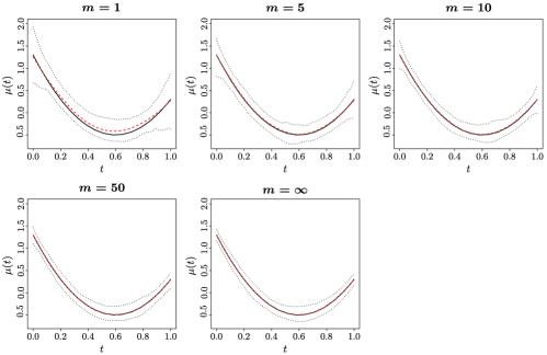
Figure 1: Estimated mean function in simulation 1. In each panel, the solid line is the true mean function, the dashed line is the pointwise mean and the two dotted lines are the pointwise $1\%$ and $99\%$ percentiles of the estimator of the mean function based on 200 runs.

The estimation results for $\mu(\cdot)$ are summarized in Figure 1, where we plot the mean and the pointwise first and 99th percentiles of the estimator. To compare with standard nonparametric regression, we also provide the estimation results for $\mu$ when $m=1$; note that in this case the covariance function is not estimable since there is no within-curve information. As can be seen, the estimation result for $m=1$ is not very different from that of $m=5$, reconfirming the nonparametric convergence rate of $\widehat{\mu}$ for sparse functional data. It is somewhat difficult to describe the estimation results of the covariance function directly. Instead, we summarize the results on $\psi_{k}(\cdot)$ and $\omega_{k}$ in Figure 2, where we plot the mean and the pointwise first and 99th percentiles of the estimated eigenfunctions. In Figure 3, we also show the empirical distributions of $\widehat{\omega}_{k}$ and $\widehat{\sigma}^{2}$. In all of the scenarios, the performance of the estimators improve with $m$; by $m=50$, all of the the estimators perform almost as well as those for $m=\infty$.

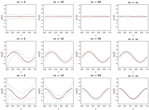
Figure 2: Estimated eigenfunctions in simulation 1. In each panel, the solid line is the eigenfunction, the dashed line is the pointwise mean and the two dotted lines are the pointwise $1\%$ and $99\%$ percentiles of the estimator of the eigenfunction in 200 runs. The three rows correspond to $\psi_{1}$, $\psi_{2}$ and $\psi_{3}$; different columns correspond to different $m$ values.

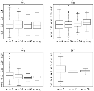
Figure 3: Box plots for $\widehat{\omega}_{1}$, $\widehat{\omega}_{2}$, $\widehat{\omega}_{3}$ and $\widehat{\sigma}^{2}$ in simulation 1.

4.2 Simulation 2

To illustrate that the proposed methods are applicable even to the cases that the trajectory of $X$ is not smooth, we now present a second simulation study where $X$ is standard Brownian motion. Again, we set the time window $[a,b]$ to be $[0,1]$. It is well known that the covariance function of $X$ is $R(s,t)=\min(s,t),s,t\in[0,1]$, which has an infinite spectral decomposition with

$$\omega_{k}=4/\{(2k-1)^{2}\pi^{2}\},\qquad\psi_{k}(t)=\sqrt{2}\sin\{(k-1/2)\pi t\},\qquad k=1,2,\ldots.$$

Again, let the observation times be $T_{ij}\sim\operatorname{Uniform}[0,1]$, $Y_{ij}=X_{i}(T_{ij})+U_{ij}$, $U_{ij}\sim\operatorname{Normal}(0,\sigma^{2})$. We let $\sigma^{2}=0.1^{2}$, which is comparable to $\omega_{3}$.

Since $X$ is not differentiable with probability one, smoothing individual trajectories is not sensible even for large $m$ values. Also, $R(s,t)$ is not differentiable on the diagonal $\{s=t\}$, and therefore the smoothness assumption in our theory is not satisfied. Nevertheless, as we will show below, the proposed method still works reasonably well. The reason is that the smoothness assumption on $R(s,t)$ in our theory is meant to guarantee the best convergence rate for the $\widehat{R}(s,t)$. When the assumption is mildly violated, the estimator may still perform well overall but may have a slower convergence rate at the nonsmooth points. A similar phenomenon was observed in Li et al. (2007), which studied kernel estimation of a stationary covariance function in a time-series setting.

We set $n=200$ and $m=5$, $10$ or $50$ in our simulations. The estimation results for the first three eigenfunctions are presented in Figure 4. Again, we plot the mean and the pointwise first and 99th percentiles of the estimated eigenfunctions. As can be seen, it is in general much harder to estimate the higher-order eigenfunctions, and the results improve as we increase $m$. The empirical distribution of the estimated eigenvalues as well as $\widehat{\sigma}^{2}$ are summarized in Figure 5. The estimated eigenvalues should be compared with the true ones, which are $(0.405,0.045,0.016)$. When $m$ is large, the estimated eigenvalues are very close to the true values.

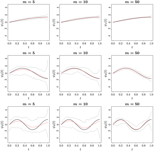
Figure 4: Estimated eigenfunctions in simulation 2. In each panel, the solid line is the eigenfunction, the dashed line is the pointwise mean and the two dotted lines are the pointwise $1\%$ and $99\%$ percentiles of the estimator of the eigenfunction in 200 runs. The three rows correspond to $\psi_{1}$, $\psi_{2}$ and $\psi_{3}$; different columns correspond to different $m$ values.

Figure 5: Box plots for $\widehat{\omega}_{1}$, $\widehat{\omega}_{2}$, $\widehat{\omega}_{3}$ and $\widehat{\sigma}^{2}$ in simulation 2.

5 Proofs

5.1 Proof of Theorem 3.1

The proof is an adaptation of familiar lines of proofs established in nonparametric function literature; see Claeskens and Van Keilegon (2003) and Härdle, Janssen and Serfling (1988). For simplicity, throughout this subsection, we abbreviate $h_{\mu}$ as $h$. Below, let $t_{1}\wedge t_{2}=\min(t_{1},t_{2})$ and $t_{1}\vee t_{2}=\max(t_{1},t_{2})$. Also define $K_{(\ell)}(t)=t^{\ell}K(t)$ and $K_{h,(\ell)}(v)=(1/h)K_{(\ell)}(v/h)$.

Lemma 1

Assume that

$$\qquad\mathbb{E}\Bigl{(}{\sup_{t\in[a,b]}}|X(t)|^{\lambda}\Bigr{)}<\infty\quad\mbox{and}\quad\mathbb{E}|U|^{\lambda}<\infty\qquad\mbox{for some $\lambda\in(2,\infty)$}.$$ (10)

Let $\mathcal{Z}_{ij}=X_{i}(T_{ij})$ or $U_{ij}$ for $1\leq i\leq n,1\leq j\leq m_{i}$. Let $c_{n}$ be any positive sequence tending to $0$ and $\beta_{n}=c_{n}^{2}+c_{n}/\gamma_{n1}$. Assume that $\beta_{n}^{-1}(\log n/n)^{1-2/\lambda}=o(1)$. Let

$$G_{n}(t_{1},t_{2}) = {1\over n}\sum_{i=1}^{n}\Biggl{\{}{1\over m_{i}}\sum_{j=1}^{m_{i}}\mathcal{Z}_{ij}I(T_{ij}\in[t_{1}\wedge t_{2},t_{1}\vee t_{2}])\Biggr{\}},$$

$$G(t_{1},t_{2}) = \mathbb{E}\{G_{n}(t_{1},t_{2})\}$$

and

$$V_{n}(t,c)={\sup_{|u|\leq c}}|G_{n}(t,t+u)-G(t,t+u)|,\qquad c>0.$$

Then

$$\sup_{t\in[a,b]}V_{n}(t,c_{n})=O(n^{-1/2}\{\beta_{n}\log n\}^{1/2})\qquad\mbox{a.s.}$$ (12)

We can obviously treat the positive and negative parts of $\mathcal{Z}_{ij}$ separately, and will assume below that $\mathcal{Z}_{ij}$ is nonnegative. Define an equally-spaced grid $\mathcal{G}:=\{v_{k}\}$, with $v_{k}=a+kc_{n}$, for $k=0,\ldots,[(b-a)/c_{n}]$, and $v_{[(b-a)/c_{n}]+1}=b$, where $[\cdot]$ denotes the greatest integer part. For any $t\in[a,b]$ and $|u|\leq c_{n}$, let $v_{k}$ be a grid point that is within $c_{n}$ of both $t$ and $t+u$, which exists. Since

$$|G_{n}(t,t+u)-G(t,t+u)| \leq |G_{n}(v_{k},t+u)-G(v_{k},t+u)|$$

$${}+|G_{n}(v_{k},t)-G(v_{k},t)|,$$

we have

$$|G_{n}(t,t+u)-G(t,t+u)|\leq 2\sup_{t\in\mathcal{G}}V_{n}(t,c_{n}).$$

Thus,

$$\sup_{t\in[a,b]}V_{n}(t,c_{n})\leq 2\sup_{t\in\mathcal{G}}V_{n}(t,c_{n}).$$ (13)

From now on, we focus on the right-hand side of (13). Let

$$a_{n}=n^{-1/2}\{\beta_{n}\log n\}^{1/2}\quad\mbox{and}\quad Q_{n}=\beta_{n}/a_{n},$$ (14)

and define $G_{n}^{\ast}(t_{1},t_{2}),G^{\ast}(t_{1},t_{2})$ and $V_{n}^{\ast}(t,c_{n})$ in the same way as $G_{n}(t_{1},t_{2})$, $G(t_{1},t_{2})$ and $V_{n}(t,c_{n})$, respectively, except with $\mathcal{Z}_{ij}I(\mathcal{Z}_{ij}\leq Q_{n})$ replacing $\mathcal{Z}_{ij}$. Then

$$\sup_{t\in\mathcal{G}}V_{n}(t,c_{n})\leq\sup_{t\in\mathcal{G}}V_{n}^{\ast}(t,c_{n})+A_{n1}+A_{n2},$$ (15)

where

$$A_{n1} = \sup_{t\in\mathcal{G}}\sup_{|u|\leq c_{n}}\bigl{(}G_{n}(t,t+u)-G_{n}^{\ast}(t,t+u)\bigr{)},$$

$$A_{n2} = \sup_{t\in\mathcal{G}}\sup_{|u|\leq c_{n}}\bigl{(}G(t,t+u)-G^{\ast}(t,t+u)\bigr{)}.$$

We first consider $A_{n1}$ and $A_{n2}$. It follows that

$$a_{n}^{-1}Q_{n}^{1-\lambda}=\{\beta_{n}^{-1}(\log n/n)^{1-2/\lambda}\}^{\lambda/2}=o(1).$$ (16)

For all $t$ and $u$, by Markov’s inequality,

$$a_{n}^{-1}\bigl{(}G_{n}(t,t+u)-G_{n}^{\ast}(t,t+u)\bigr{)}$$

$$\qquad\leq a_{n}^{-1}{1\over n}\sum_{i=1}^{n}\Biggl{\{}{1\over m_{i}}\sum_{j=1}^{m_{i}}\mathcal{Z}_{ij}I(\mathcal{Z}_{ij}>Q_{n})\Biggr{\}}$$

$$\qquad\leq a_{n}^{-1}Q_{n}^{1-\lambda}{1\over n}\sum_{i=1}^{n}\Biggl{\{}{1\over m_{i}}\sum_{j=1}^{m_{i}}\mathcal{Z}_{ij}^{\lambda}I(\mathcal{Z}_{ij}>Q_{n})\Biggr{\}}$$

$$\qquad\leq a_{n}^{-1}Q_{n}^{1-\lambda}{1\over n}\sum_{i=1}^{n}\Biggl{\{}{1\over m_{i}}\sum_{j=1}^{m_{i}}\mathcal{Z}_{ij}^{\lambda}\Biggr{\}}.$$

Consider the case $\mathcal{Z}_{ij}=X_{i}(T_{ij})$, the other case being simpler. It follows that

$${1\over m_{i}}\sum_{j=1}^{m_{i}}\mathcal{Z}_{ij}^{\lambda}\leq W_{i}\qquad\mbox{where }W_{i}={\sup_{t\in[a,b]}}|X_{i}(t)|^{\lambda}.$$

Thus,

$$a_{n}^{-1}\bigl{(}G_{n}(t,t+u)-G_{n}^{\ast}(t,t+u)\bigr{)}\leq a_{n}^{-1}Q_{n}^{1-\lambda}{1\over n}\sum_{i=1}^{n}W_{i}.$$ (17)

By the SLLN, $n^{-1}\sum_{i=1}^{n}W_{i}\stackrel{{\scriptstyle\mathrm{a.s.}}}{{\longrightarrow}}\mathbb{E}(\sup_{t\in[a,b]}|X(t)|^{\lambda})<\infty$. By (16) and (17), $a_{n}^{-1}A_{n1}\stackrel{{\scriptstyle\mathrm{a.s.}}}{{\longrightarrow}}0$. By (16) and (17) again, $a_{n}^{-1}A_{n2}=0$, and so we have proved

$$\lim_{n\to\infty}(A_{n1}+A_{n2})=o(a_{n})\qquad\mbox{a.s.}$$ (18)

To bound $V_{n}^{\ast}(t,c_{n})$ for a fixed $t\in\mathcal{G}$, we perform a further partition. Define $w_{n}=[Q_{n}c_{n}/a_{n}+1]$ and $u_{r}=rc_{n}/w_{n}$, for $r=-w_{n},-w_{n}+1,\ldots,w_{n}$. Note that $G_{n}^{\ast}(t,t+u)$ is monotone in $|u|$ since $\mathcal{Z}_{ij}\geq 0$. Suppose that $0\leq u_{r}\leq u\leq u_{r+1}$. Then

$$G_{n}^{\ast}(t,t+u_{r})-G^{\ast}(t,t+u_{r})+G^{\ast}(t,t+u_{r})-G^{\ast}(t,t+u_{r+1})$$

$$\qquad\leq G_{n}^{\ast}(t,t+u)-G^{\ast}(t,t+u)$$

$$\qquad\leq G_{n}^{\ast}(t,t+u_{r+1})-G^{\ast}(t,t+u_{r+1})+G^{\ast}(t,t+u_{r+1})-G^{\ast}(t,t+u_{r}),$$

from which we conclude that

$$|G_{n}^{\ast}(t,t+u)-G^{\ast}(t,t+u)|\leq\max(\xi_{nr},\xi_{n,r+1})+G^{\ast}(t+u_{r},t+u_{r+1}),$$

where

$$\xi_{nr}=|G_{n}^{\ast}(t,t+u_{r})-G^{\ast}(t,t+u_{r})|.$$

The same holds if $u_{r}\leq u\leq u_{r+1}\leq 0$. Thus,

$$V_{n}^{\ast}(t,c_{n})\leq\max_{-w_{n}\leq r\leq w_{n}}\xi_{nr}+\max_{-w_{n}\leq r\leq w_{n}}G^{\ast}(t+u_{r},t+u_{r+1}).$$

For all $r$,

$$G^{\ast}(t+u_{r},t+u_{r+1}) \leq Q_{n}\mathbb{P}(t+u_{r}\leq T\leq t+u_{r+1})$$

$$\leq M_{T}Q_{n}(u_{r+1}-u_{r})\leq M_{T}a_{n}.$$

Therefore, for any $B$,

$$\mathbb{P}\{V_{n}^{\ast}(t,c_{n})\geq Ba_{n}\}\leq\mathbb{P}\Bigl{\{}\max_{-w_{n}\leq r\leq w_{n}}\xi_{nr}\geq(B-M_{T})a_{n}\Bigr{\}}.$$ (19)

Now let $Z_{i}=m_{i}^{-1}\sum_{j=1}^{m_{i}}\mathcal{Z}_{ij}I(\mathcal{Z}_{ij}\leq Q_{n})I(T_{ij}\in(t,t+u_{r}])$ so that $\xi_{nr}=|{1\over n}\times\sum_{i=1}^{n}\{Z_{i}-\mathbb{E}(Z_{i})\}|$. We have $|Z_{i}-\mathbb{E}(Z_{i})|\leq Q_{n}$, and

$$\sum_{i=1}^{n}\operatorname{var}(Z_{i})\leq\sum_{i=1}^{n}\mathbb{E}Z_{i}^{2}\leq M\sum_{i=1}^{n}(c_{n}^{2}+c_{n}/m_{i})\leq Mn\beta_{n}$$

for some finite $M$. By Bernstein’s inequality,

$$\mathbb{P}\{\xi_{nr}\geq(B-M_{T})a_{n}\} \leq \exp\biggl{\{}-{(B-M_{T})^{2}n^{2}a_{n}^{2}\over 2\sum_{i=1}^{n}\operatorname{var}(Z_{i})+(2/3)(B-M_{T})Q_{n}na_{n}}\biggr{\}}$$

$$\leq \exp\biggl{\{}-{(B-M_{T})^{2}n^{2}a_{n}^{2}\over 2Mn\beta_{n}+(2/3)(B-M_{T})n\beta_{n}}\biggr{\}}\leq n^{-B^{\ast}},$$

where $B^{\ast}={(B-M_{T})^{2}\over 2M+(2/3)(B-M_{T})}$. By (19) and Boole’s inequality,

$$\mathbb{P}\Bigl{\{}\sup_{t\in\mathcal{G}}V_{n}^{\ast}(t,c_{n})\geq Ba_{n}\Bigr{\}}\!\leq\!\biggl{(}\biggl{[}{b-a\over c_{n}}\biggr{]}+1\biggr{)}\!\biggl{(}2\biggl{[}{Q_{n}c_{n}\over a_{n}}+1\biggr{]}+1\biggr{)}n^{-B^{\ast}}\!\leq\!C{Q_{n}\over a_{n}}n^{-B^{\ast}}$$

for some finite $C$. Now $Q_{n}/a_{n}=\beta_{n}/a_{n}^{2}=n/\log n$. So $\mathbb{P}\{V_{n}^{\ast}(t,c_{n})\geq Ba_{n}\}$ is summable in $n$ if we select $B$ large enough such that $B^{\ast}>2$. By the Borel–Cantelli lemma,

$$\sup_{t\in\mathcal{G}}V_{n}^{\ast}(t,c_{n})=O(a_{n})\qquad\mbox{a.s.}$$ (20)

Hence, (12) follows from combining (13), (15), (18) and (20).

Lemma 2

Let $\mathcal{Z}_{ij}$ be as in Lemma 1 and assume that (10) holds. Let $h=h_{n}$ be a bandwidth and let $\beta_{n}=h^{2}+h/\gamma_{n1}$. Assume that $h\to 0$ and $\beta_{n}^{-1}(\log n/n)^{1-2/\lambda}=o(1)$ For any nonnegative integer $p$, let

$$D_{p,n}(t)={1\over n}\sum_{i=1}^{n}\Biggl{[}{1\over m_{i}}\sum_{j=1}^{m_{i}}K_{h,(p)}(T_{ij}-t)\mathcal{Z}_{ij}\Biggr{]}.$$

Then we have

$$\sup_{t\in[a,b]}\sqrt{nh^{2}/(\beta_{n}\log n)}|D_{p,n}(t)-\mathbb{E}\{D_{p,n}(t)\}|=O(1)\qquad\mbox{a.s.}$$

Since both $K$ and $t^{p}$ are bounded variations, $K_{(p)}$ is also a bounded variation. Thus, we can write $K_{(p)}=K_{(p),1}-K_{(p),2}$ where $K_{(p),1}$ and $K_{(p),2}$ are both increasing functions; without loss of generality, assume that $K_{(p),1}(-1)=K_{(p),2}(-1)=0$. Below, we apply Lemma 1 by letting $c_{n}=2h$. It is clear that the assumptions of Lemma 1 hold here. Write

$$D_{n}(t) = {1\over n}\sum_{i=1}^{n}\Biggl{\{}{1\over m_{i}}\sum_{j=1}^{m_{i}}K_{h,(p)}(T_{ij}-t)\mathcal{Z}_{ij}\Biggr{\}}$$

$$= {1\over n}\sum_{i=1}^{n}\Biggl{\{}{1\over m_{i}}\sum_{j=1}^{m_{i}}\mathcal{Z}_{ij}I(-h\leq T_{ij}-t\leq h)\int_{-h}^{T_{ij}-t}dK_{h,(p)}(v)\Biggr{\}}$$

$$= \int_{-h}^{h}{1\over n}\sum_{i=1}^{n}\Biggl{\{}{1\over m_{i}}\sum_{j=1}^{m_{i}}\mathcal{Z}_{ij}I(v\leq T_{ij}-t\leq h)\Biggr{\}}\,dK_{h,(p)}(v)$$

$$= \int_{-h}^{h}G_{n}(t+v,t+h)\,dK_{h,(p)}(v),$$

where $G_{n}$ is as defined in (1). We have

$${\sup_{t\in[a,b]}}|D_{p,n}(t)-\mathbb{E}\{D_{p,n}(t)\}|$$

$$\qquad\leq\sup_{t\in[a,b]}V_{n}(t,2h)\int_{-h}^{h}\bigl{|}dK_{h,(p)}\bigr{|}$$ (21)

$$\qquad\leq\bigl{\{}K_{(p),1}(1)+K_{(p),2}(1)\bigr{\}}h^{-1}\sup_{t\in[a,b]}V_{n}(t,2h),$$

and the conclusion of the lemma follows from Lemma 1. Proof of Theorem 3.1 Define

$$R_{r}^{\ast}=R_{r}-\mu(t)S_{r}-h\mu^{(1)}(t)S_{r+1}.$$

By straightforward calculations, we have

$$\widehat{\mu}(t)-\mu(t)={R_{0}^{\ast}S_{2}-R_{1}^{\ast}S_{1}\over S_{0}S_{2}-S_{1}^{2}},$$ (22)

where $S_{0},S_{1},S_{2}$ are defined as in (1). Write

$$R_{r}^{\ast} = {1\over n}\sum_{i}\Biggl{[}{1\over m_{i}}\sum_{j=1}^{m_{i}}K_{h}(T_{ij}-t)\{(T_{ij}-t)/h\}^{r}\bigl{\{}Y_{ij}-\mu(t)-\mu^{(1)}(t)(T_{ij}-t)\bigr{\}}\Biggr{]}$$

$$= {1\over n}\sum_{i}\Biggl{[}{1\over m_{i}}\sum_{j=1}^{m_{i}}K_{h}(T_{ij}-t)\{(T_{ij}-t)/h\}^{r}$$

$$\hskip 60.3pt{}\times\bigl{\{}\varepsilon_{ij}+\mu(T_{ij})-\mu(t)-\mu^{(1)}(t)(T_{ij}-t)\bigr{\}}\Biggr{]}.$$

By Taylor’s expansion and Lemma 2, uniformly in $t$,

$$R_{r}^{\ast}={1\over n}\sum_{i}{1\over m_{i}}\sum_{j}K_{h}(T_{ij}-t)\{(T_{ij}-t)/h\}^{r}\varepsilon_{ij}+O(h^{2}),$$ (23)

and it follows from Lemma 2 that

$$R_{i}^{\ast}=O\bigl{(}h^{2}+\delta_{n1}(h)\bigr{)}\qquad\mbox{a.s.}$$ (24)

Now, at any interior point $t\in[a+h,b-h]$, since $f$ has a bounded derivative,

$$\mathbb{E}\{S_{0}\} = \int_{-1}^{1}K(v)f(t+hv)\,dv=f(t)+O(h),$$

$$\mathbb{E}\{S_{1}\} = O(h),\qquad\mathbb{E}\{S_{2}\}=f(t)\nu_{2}+O(h),$$

where $\nu_{2}=\int v^{2}K(v)\,dv$. By Lemma 2, we conclude that, uniformly for $t\in[a+h,b-h]$,

$$S_{0} = f(t)+O\bigl{(}h+\delta_{n1}(h)\bigr{)},\qquad S_{1}=O\bigl{(}h+\delta_{n1}(h)\bigr{)},$$

$$S_{2} = f(t)\nu_{2}+O\bigl{(}h+\delta_{n1}(h)\bigr{)}.$$

Thus, the rate in the theorem is established by applying (22). The same rate can also be similarly seen to hold for boundary points.

5.2 Proofs of Theorems 3.3 and 3.4

Lemma 3

Assume that

$$\mathbb{E}\Bigl{(}{\sup_{t\in[a,b]}}|X(t)|^{2\lambda}\Bigr{)}<\infty\quad\mbox{and}\quad\mathbb{E}|U|^{2\lambda}<\infty\qquad\mbox{for some $\lambda\in(2,\infty)$}.$$ (26)

Let $\mathcal{Z}_{ijk}$ be $X(T_{ij})X(T_{ik})$, $X(T_{ij})U_{ik}$ or $U_{ij}U_{ik}$. Let $c_{n}$ be any positive sequence tending to $0$ and $\beta_{n}=c_{n}^{4}+c_{n}^{3}/\gamma_{n1}+c_{n}^{2}/\gamma_{n2}$. Assume that$\beta_{n}^{-1}(\log n/n)^{1-2/\lambda}=o(1)$. Let

$$G_{n}(s_{1},t_{1},s_{2},t_{2})$$

$$\qquad={1\over n}\sum_{i=1}^{n}\biggl{\{}{1\over N_{i}}\sum_{k\not=j}\mathcal{Z}_{ijk}I(T_{ij}\in[s_{1}\wedge s_{2},s_{1}\vee s_{2}],$$ (27)

$$\hskip 133.0ptT_{ik}\in[t_{1}\wedge t_{2},t_{1}\vee t_{2}])\biggr{\}},$$

$G(s_{1},t_{1},s_{2},t_{2})=\mathbb{E}\{G_{n}(s_{1},t_{1},s_{2},t_{2})\}$ and

$$V_{n}(s,t,\delta)={\sup_{|u_{1}|,|u_{2}|\leq\delta}}|G_{n}(s,t,s+u_{1},t+u_{2})-G(s,t,s+u_{1},t+u_{2})|.$$

Then

$$\sup_{s,t\in[a,b]}V_{n}(s,t,c_{n})=O(n^{-1/2}\{\beta_{n}\log n\}^{1/2})\qquad\mbox{a.s.}$$

The proof is similar to that of Lemma 1, and so we only outline the main differences. Let $a_{n},Q_{n}$ be as in (14). Let $\mathcal{G}$ be a two-dimensional grid on $[a,b]^{2}$ with mesh $c_{n}$, that is, $\mathcal{G}=\{(v_{k_{1}},v_{k_{2}})\}$ where $v_{k}$ is defined as in the proof of Lemma 1. Then we have

$$\sup_{s,t\in[a,b]}V_{n}(s,t,c_{n})\leq 4\sup_{(s,t)\in\mathcal{G}}V_{n}(s,t,c_{n}).$$ (28)

Define $G_{n}^{*}(s_{1},t_{1},s_{2},t_{2}),G^{\ast}(s_{1},t_{1},s_{2},t_{2})$ and $V_{n}^{\ast}(s,t,\delta)$ in the same way as $G_{n}(s_{1},t_{1},s_{2},t_{2})$, $G(s_{1},t_{1}$, $s_{2},t_{2})$ and $V_{n}(s,t,\delta)$ except with $\mathcal{Z}_{ijk}I(\mathcal{Z}_{ijk}\leq Q_{n})$ replacing $\mathcal{Z}_{ijk}$. Then

$$\sup_{(s,t)\in\mathcal{G}}V_{n}(s,t,c_{n})\leq\sup_{(s,t)\in\mathcal{G}}V^{\ast}_{n}(s,t,c_{n})+A_{n1}+A_{n2},$$ (29)

where

$$A_{n1} = {\sup_{(s,t)\in\mathcal{G}}\sup_{|u_{1}|,|u_{2}|\leq c_{n}}}|G_{n}(s,t,s+u_{1},t+u_{2})-G_{n}^{\ast}(s,t,s+u_{1},t+u_{2})|,$$

$$A_{n2} = {\sup_{(s,t)\in\mathcal{G}}\sup_{|u_{1}|,|u_{2}|\leq c_{n}}}|G(s,t,s+u_{1},t+u_{2})-G^{\ast}(s,t,s+u_{1},t+u_{2})|.$$

Using the technique similar to that in the proof of Lemma 1, we can show $A_{n1}$ and $A_{n2}$ is $o(a_{n})$ almost surely. To bound $V_{n}^{\ast}(s,t,c_{n})$ for fixed $(s,t)$, we create a further partition. Put $w_{n}=[Q_{n}c_{n}/a_{n}+1]$ and $u_{r}=rc_{n}/w_{n},r=-w_{n},\ldots,w_{n}$. Then

$$V_{n}^{\ast}(s,t,c_{n}) \leq \max_{-w_{n}\leq r_{1},r_{2}\leq w_{n}}\xi_{n,r_{1},r_{2}}$$

$${}+\max_{-w_{n}\leq r_{1},r_{2}\leq w_{n}}\{G^{\ast}(s,t,s+u_{r_{1}+1},t+u_{r_{2}+1})$$

$$\hskip 81.23pt{}-G^{\ast}(s,t,s+u_{r_{1}},t+u_{r_{2}})\},$$

where

$$\xi_{n,r_{1},r_{2}}=|G_{n}^{\ast}(s,t,s+u_{r_{1}},t+u_{r_{2}})-G^{\ast}(s,t,s+u_{r_{1}},t+u_{r_{2}})|.$$

It is easy to see that $\operatorname{var}(\xi_{n,r_{1},r_{2}})\leq Mn\beta_{n}$ for some finite $M$, and the rest of the proof completely mirrors that of Lemma 1 and is omitted.

Lemma 4

Let $\mathcal{Z}_{ijk}$ be as in Lemma 3 and assume that (26) holds. Let $h=h_{n}$ be a bandwidth and let $\beta_{n}=h^{4}+h^{3}/\gamma_{n1}+h^{2}/\gamma_{n2}$. Assume that $h\to 0$ and $\beta_{n}^{-1}(\log n/n)^{1-2/\lambda}=o(1)$. For any nonnegative integers $p,q$, let

$$D_{p,q,n}(s,t)={1\over n}\sum_{i=1}^{n}\biggl{[}{1\over N_{j}}\sum_{k\not=j}\mathcal{Z}_{ijk}K_{h,(p)}(T_{ij}-s)K_{h,(q)}(T_{ik}-t)\biggr{]}.$$

Then, for any $p,q$,

$$\sup_{s,t\in[a,b]}\sqrt{nh^{4}/(\beta_{n}\log n)}|D_{p,q,n}(s,t)-\mathbb{E}\{D_{p,q,n}(s,t)\}|=O(1)\qquad\mbox{a.s.}$$

Write

$$D_{p,q,n}(s,t)$$

$$\qquad=\sum_{i=1}^{n}\biggl{[}{1\over N_{i}}\sum_{k\not=j}\mathcal{Z}_{ijk}I(T_{ij}\leq s+h)I(T_{ik}\leq t+h)$$

$$\qquad\quad\hskip 51.0pt{}\times K_{h,(p)}(T_{ij}-s)K_{h,(q)}(T_{ik}-t)\biggr{]}$$

$$\qquad=\int\int_{(u,v)\in[-h,h]^{2}}{1\over n}\sum_{i=1}^{n}\biggl{[}{1\over N_{i}}\sum_{k\not=j}\mathcal{Z}_{ijk}$$

$$\qquad\quad\hskip 121.7pt{}\times I(T_{ij}\in[s+u,s+h])$$

$$\qquad\quad\hskip 122.5pt{}\times I(T_{ik}\in[t+v,t+h])\biggr{]}\,dK_{h,(p)}(u)\,dK_{h,(q)}(v)$$

$$\qquad=\int\int_{(u,v)\in[-h,h]^{2}}G_{n}(s+u,t+v,s+h,t+h)\,dK_{h,(p)}(u)dK_{h,(q)}(v),$$

where $G_{n}$ is as in (3). Now,

$${\sup_{(s,t)\in[a,b]^{2}}}|D_{p,q,n}(s,t)-\mathbb{E}\{D_{p,q,n}(s,t)\}|$$

$$\qquad\leq\sup_{s,t\in[a,b]}V_{n}(s,t,2h)\int\int_{(u,v)\in[-h,h]^{2}}\bigl{|}d\bigl{\{}K_{h,(p)}(u)\bigr{\}}\bigr{|}\bigl{|}d\bigl{\{}K_{h,(q)}(v)\bigr{\}}\bigr{|}$$

$$\qquad=O[\{\beta_{n}\log n/(nh^{4})\}^{1/2}]\qquad\mbox{a.s.}$$

by Lemma 3, using the same argument as in (5.1). Proof of Theorem 3.3 Let $S_{pq},R_{pq},\mathcal{A}_{i}$ and $\mathcal{B}$ be defined as in (3). Also, for $p,q\geq 0$, define

$$R_{pq}^{\ast}=R_{pq}-C(s,t)S_{pq}-h_{R}C^{(1,0)}(s,t)S_{p+1,q}-h_{R}C^{(0,1)}(s,t)S_{p,q+1}.$$

By straightforward algebra, we have

$$(\widehat{C}-C)(s,t)=(\mathcal{A}_{1}R_{00}^{\ast}-\mathcal{A}_{2}R_{10}^{\ast}-\mathcal{A}_{3}R_{01}^{\ast})\mathcal{B}^{-1}.$$ (30)

By standard calculations, we have the following rates uniformly on $[a+h_{R},b-h_{R}]^{2}$:

$$\mathbb{E}(S_{00}) = f(s)f(t)+O(h_{R}),\qquad\mathbb{E}(S_{01})=O(h_{R}),$$

$$\mathbb{E}(S_{10}) = O(h_{R}),\qquad\mathbb{E}(S_{02})=f(s)f(t)\nu_{2}+O(h_{R}),$$

$$\mathbb{E}(S_{20}) = f(s)f(t)\nu_{2}+O(h_{R}),\qquad\mathbb{E}(S_{11})=O(h_{R}).$$

By these and Lemma 4, we have the following almost sure uniform rates:

$$\mathcal{A}_{1} = f^{2}(s)f^{2}(t)\nu_{2}^{2}+O\bigl{(}h_{R}+\delta_{n2}(h_{R})\bigr{)},$$

$$\mathcal{A}_{2} = O\bigl{(}h_{R}+\delta_{n2}(h_{R})\bigr{)},$$

$$\mathcal{A}_{3} = O\bigl{(}h_{R}+\delta_{n2}(h_{R})\bigr{)},$$

$$\mathcal{B} = f^{3}(s)f^{3}(t)\nu_{2}^{2}+O\bigl{(}h_{R}+\delta_{n2}(h_{R})\bigr{)}.$$

To analyze the behavior of the components of (30), it suffices now to analyze $R_{pq}^{\ast}$. Write

$$R_{00}^{\ast} = {1\over n}\sum_{i=1}^{n}\biggl{[}{1\over N_{i}}\sum_{k\not=j}\bigl{\{}Y_{ij}Y_{ik}-C(s,t)$$

$$\hskip 64.35pt{}-C^{(1,0)}(s,t)(T_{ij}-s)$$

$$\hskip 64.35pt{}-C^{(0,1)}(s,t)(T_{ik}-t)\bigr{\}}\times K_{h_{R}}(T_{ij}-s)K_{h_{R}}(T_{ik}-t)\biggr{]}.$$

Let $\varepsilon_{ijk}^{\ast}=Y_{ij}Y_{ik}-C(T_{ij},T_{ik})$. By Taylor’s expansion,

$$Y_{ij}Y_{ik}-C(s,t)-C^{(1,0)}(s,t)(T_{ij}-s)-C^{(0,1)}(s,t)(T_{ik}-t)$$

$$\qquad=Y_{ij}Y_{ik}-C(s,t)-C(T_{ij},T_{ik})+C(T_{ij},T_{ik})$$

$$\qquad\quad{}-C^{(1,0)}(s,t)(T_{ij}-s)-C^{(0,1)}(s,t)(T_{ik}-t)$$

$$\qquad=\varepsilon_{ijk}^{\ast}+O(h_{R}^{2})\qquad\mbox{a.s.}$$

It follows that

$$R_{00}^{\ast}={1\over n}\sum_{i=1}^{n}{1\over N_{i}}\sum_{k\not=j}\varepsilon_{ijk}^{\ast}K_{h_{R}}(T_{ij}-s)K_{h_{R}}(T_{ik}-t)+O(h_{R}^{2}).$$ (32)

Applying Lemma 4, we obtain, uniformly in $s,t$,

$$R_{00}^{\ast}=O\bigl{(}\delta_{n2}(h_{R})+h_{R}^{2}\bigr{)}\qquad\mbox{a.s.}$$ (33)

By (5.2),

$$\mathcal{A}_{1}\mathcal{B}^{-1}=[f(s)f(t)]^{-1}+O\bigl{(}h_{R}+\delta_{n2}(h_{R})\bigr{)}.$$ (34)

Thus, $R_{00}^{\ast}\mathcal{A}_{1}\mathcal{B}^{-1}=O(\delta_{n2}(h_{R})+h_{R}^{2})$ a.s. Similar derivations show that$R_{10}^{\ast}\mathcal{A}_{2}\times\mathcal{B}^{-1}$ and $R_{01}^{\ast}\mathcal{A}_{3}\mathcal{B}^{-1}$ are both of lower order. Thus, the rate in (7) is obtained for $s,t\in[a+h_{R},b-h_{R}]$. As for $s$ and/or $t$ in $[a,a+h)\cup(b-h,b]$, similar calculations show that the same rate also holds. The result follows by taking into account of the rate of $\widehat{\mu}$. Proof of Theorem 3.4 Note that

$$\widehat{\sigma}^{2}-\sigma^{2}={1\over b-a}\int_{a}^{b}\{\widehat{V}(t)-V(t)\}\,dt-{1\over b-a}\int_{a}^{b}\{\widehat{C}(t,t)-C(t,t)\}\,dt.$$

To consider $\widehat{V}(t)-V(t)$ we follow the development in the proof of Theorem 3.1. Recall (4) and let $Q_{r}^{\ast}=Q_{r}-V(t)S_{r}-hV^{(1)}(t)S_{r+1}$. Then, as in (22), we obtain

$$\widehat{V}(t)-V(t)={Q_{0}^{\ast}S_{2}-Q_{1}^{\ast}S_{1}\over S_{0}S_{2}-S_{1}^{2}}.$$

Write

$$Q_{r}^{\ast} = {1\over n}\sum_{i=1}^{n}{1\over m_{i}}\sum_{j=1}^{m_{i}}K_{h_{V}}(T_{ij}-t)\{(T_{ij}-t)/h_{V}\}^{r}\bigl{\{}Y_{ij}^{2}-V(t)-V^{(1)}(t)(T_{ij}-t)\bigr{\}}$$

$$= {1\over n}\sum_{i=1}^{n}{1\over m_{i}}\sum_{j=1}^{m_{i}}K_{h_{V}}(T_{ij}-t)\{(T_{ij}-t)/h\}^{r}\{Y_{ij}^{2}-V(T_{ij})\}+O(h_{V}^{2}),$$

which, by Lemma 1, has the uniformly rate $O(h_{V}^{2}+\delta_{n1}(h_{V}))$ a.s. By (5.1), we have

$$\widehat{V}(t)-V(t) = {1\over f(t)n}\sum_{i}{1\over m_{i}}\sum_{j=1}^{m_{i}}K_{h}(T_{ij}-t)\{Y_{ij}^{2}-V(T_{ij})\}$$

$${}+O\bigl{(}h_{V}^{2}+\delta_{n1}^{2}(h_{V})\bigr{)}\qquad\mbox{a.s.}$$

Thus,

$$\int_{a}^{b}\{\widehat{V}(t)-V(t)\}\,dt = {1\over n}\sum_{i=1}^{n}{1\over m_{i}}\sum_{j=1}^{m_{i}}\{Y_{ij}^{2}-V(T_{ij})\}\int_{a}^{b}K_{h_{V}}(T_{ij}-t)f^{-1}(t)\,dt$$

$${}+O\bigl{(}h_{V}^{2}+\delta_{n1}^{2}(h_{V})\bigr{)}\qquad\mbox{a.s.}$$

Note that

$$\biggl{|}\int_{a}^{b}K_{h_{V}}(T_{ij}-t)f^{-1}(t)\,dt\biggr{|}\leq\sup_{t}f^{-1}(t).$$

By Lemma 5 below in this subsection,

$$\quad\int_{a}^{b}\{\widehat{V}(t)-V(t)\}\,dt=O\bigl{(}(\log n/n)^{1/2}+h_{V}^{2}+\delta_{n1}^{2}(h_{V})\bigr{)}\qquad\mbox{a.s.}$$ (35)

Next, we consider $\widehat{C}(t,t)-C(t,t)$. We apply (30) but will focus on $R_{00}^{\ast}\mathcal{A}_{1}\mathcal{B}^{-1}$ since the other two terms are dealt with similarly. By (32)–(34),

$$\quad R_{00}^{\ast}\mathcal{A}_{1}\mathcal{B}^{-1} = {1\over f(s)f(t)n}\sum_{i=1}^{n}{1\over N_{i}}\sum_{k\not=j}\varepsilon_{ijk}^{\ast}K_{h_{R}}(T_{ij}-s)K_{h_{R}}(T_{ik}-t)$$

$${}+O\bigl{(}h_{R}^{2}+\delta_{n2}^{2}(h_{R})\bigr{)}\qquad\mbox{a.s.}$$

Thus,

$$\int_{a}^{b}\{\widehat{C}(t,t)-C(t,t)\}\,dt$$

$$\qquad={1\over n}\sum_{i=1}^{n}{1\over N_{i}}\sum_{k\not=j}\varepsilon_{ijk}^{\ast}\int_{a}^{b}K_{h_{R}}(T_{ij}-t)K_{h_{R}}(T_{ik}-t)f^{-2}(t)\,dt$$

$$\qquad\quad{}+O\bigl{(}h_{R}^{2}+\delta_{n2}^{2}(h_{R})\bigr{)}\qquad\mbox{a.s.}$$

Write

$$\int_{a}^{b}K_{h_{R}}(T_{ij}-t)K_{h_{R}}(T_{ik}-t)f^{-2}(t)\,dt$$

$$\qquad=\int_{-1}^{1}K(u)K_{h_{R}}\bigl{(}(T_{ik}-T_{ij})+uh_{R}\bigr{)}f^{-2}(T_{ij}-uh_{R})\,du.$$

A slightly modified version of Lemma 1 leads to the “one-dimensional” rate:

$$\sup_{u\in[0,1]}\Biggl{|}{1\over n}\sum_{i=1}^{n}{1\over N_{i}}\sum_{k\not=j}\varepsilon_{ijk}^{\ast}K_{h_{R}}\bigl{(}(T_{ik}-T_{ij})+uh_{R}\bigr{)}f^{-2}(T_{ij}-uh_{R})\Biggr{|}$$

$$\qquad=O(\delta_{n1}(h_{R}))\qquad\mbox{a.s.}$$

It follows that

$$\quad\int_{a}^{b}\{\widehat{C}(t,t)-C(t,t)\}\,dt=O\bigl{(}h_{R}^{2}+\delta_{n1}(h_{R})+\delta_{n2}^{2}(h_{R})\bigr{)}\qquad\mbox{a.s.}$$ (37)

The theorem follows from (35) and (37).

Lemma 5

Assume that $\xi_{ni},1\leq i\leq n$, are independent random variables with mean zero and finite variance. Also assume that there exist i.i.d. random variables $\xi_{i}$ with mean zero and finite $\delta$th moment for some $\delta>2$ such that $|\xi_{ni}|\leq|\xi_{i}|$. Then

$${1\over n}\sum_{i=1}^{n}\xi_{ni}=O\bigl{(}(\log n/n)^{1/2}\bigr{)}\qquad\mbox{a.s.}$$

Let $a_{n}=(\log n/n)^{1/2}$. Assume that $\xi_{ni}\geq 0$. Write

$$\xi_{ni}=\xi_{ni\succ}+\xi_{ni\prec}:=\xi_{ni}I(|\xi_{ni}|>a_{n}^{-1})+\xi_{ni}I(|\xi_{ni}|\leq a_{n}^{-1}).$$

Then

$$\Biggl{|}{1\over a_{n}n}\sum_{i=1}^{n}\xi_{ni\succ}\Biggr{|}\leq{1\over a_{n}n}\sum_{i=1}^{n}|\xi_{ni\succ}|^{\delta}|\xi_{ni\succ}|^{1-\delta}\leq a_{n}^{\delta-2}{1\over n}\sum_{i=1}^{n}|\xi_{i}|^{\delta}\to 0\qquad\mbox{a.s.}$$

by the law of large numbers. The mean of the left-hand side is also tending to zero by the same argument. Thus, $n^{-1}\sum_{i=1}^{n}(\xi_{ni\succ}-\mathbb{E}\{\xi_{ni\succ}\})=o(a_{n})$. Next, by Bernstein’s inequality,

$$\mathbb{P}\Biggl{(}{1\over n}\sum_{i=1}^{n}(\xi_{ni\prec}-\mathbb{E}\{\xi_{ni\prec}\})>Ba_{n}\Biggr{)} \leq \exp\biggl{\{}-{B^{2}n^{2}a_{n}^{2}\over 2n\sigma^{2}+(2/3)Bn}\biggr{\}}$$

$$= \exp\biggl{\{}-{B^{2}\log n\over 2\sigma^{2}+(2/3)B}\biggr{\}},$$

which is summable for large enough $B$. The result follows from the Borel–Cantelli lemma.

5.3 Proof of Theorem 3.6

Let $\Delta$ be the integral operator with kernel $\widehat{R}-R$.

Lemma 6

For any bounded measurable function $\psi$ on $[a,b]$,

$${\sup_{t\in[a,b]}}|(\Delta\psi)(t)|=O\bigl{(}h_{\mu}^{2}+\delta_{n1}(h_{\mu})+h_{R}^{2}+\delta_{n1}(h_{R})+\delta_{n2}^{2}(h_{R})\bigr{)}\qquad\mbox{a.s.}$$

It follows that

$$(\Delta\psi)(t) = \int_{s=a}^{b}(\widehat{C}-C)(s,t)\psi(s)\,ds-\int_{s=a}^{b}\{\widehat{\mu}(s)\widehat{\mu}(t)-\mu(s)\mu(t)\}\psi(s)\,ds$$

$$= \!:A_{n1}-A_{n2}.$$

By (30),

$$A_{n1}=\int_{s=a}^{b}(\mathcal{A}_{1}R_{00}^{\ast}-\mathcal{A}_{2}R_{10}^{\ast}-\mathcal{A}_{3}R_{01}^{\ast})\mathcal{B}^{-1}\psi(s)\,ds.$$

We focus on $\int_{s=a}^{b}\mathcal{A}_{1}R_{00}^{\ast}\mathcal{B}^{-1}\psi(s)\,ds$ since the other two terms are of lower order and can be dealt with similarly. By (32) and (34),

$$\int_{s=a}^{b}\mathcal{A}_{1}R_{00}^{\ast}\mathcal{B}^{-1}\psi(s)\,ds$$

$$\qquad={1\over f(t)n}\sum_{i=1}^{n}{1\over N_{i}}\sum_{k\not=j}\varepsilon_{ijk}^{\ast}K_{h_{R}}(T_{ik}-t)\int_{s=a}^{b}K_{h_{R}}(T_{ij}-s)\psi(s)f(s)^{-1}\,ds$$

$$\qquad\quad{}+O\bigl{(}h_{R}^{2}+\delta_{n2}^{2}(h_{R})\bigr{)}.$$

Note that

$$\biggl{|}\int_{s=a}^{b}K_{h_{R}}(T_{ij}-s)\psi(s)f(s)^{-1}\,ds\biggr{|}\leq\sup_{s\in[a,b]}(|\psi(s)|f(s)^{-1})\int_{u=-1}^{1}K(u)\,du.$$

Thus, Lemma 1 can be easily improvised to give the following uniform rate over $t$:

$${1\over f(t)n}\sum_{i=1}^{n}{1\over N_{i}}\sum_{k\not=j}\varepsilon_{ijk}^{\ast}K_{h_{R}}(T_{ik}-t)\int_{s=a}^{b}K_{h_{R}}(T_{ij}-s)\psi(s)f(s)^{-1}\,ds$$

$$\qquad=O(\delta_{n1}(h_{R}))\qquad\mbox{a.s.}$$

Thus,

$$\int_{s=a}^{b}\mathcal{A}_{1}R_{00}^{\ast}\mathcal{B}^{-1}\psi(s)\,ds=O\bigl{(}\delta_{n1}(h_{R})+h_{R}^{2}+\delta_{n2}^{2}(h_{R})\bigr{)}\qquad\mbox{a.s.},$$

which is also the rate of $A_{n1}$. Next, we write

$$A_{n2}=\widehat{\mu}(t)\int_{s=a}^{b}\{\widehat{\mu}(s)-\mu(s)\}\psi(s)\,ds-\{\widehat{\mu}(t)-\mu(t)\}\int_{s=a}^{b}\mu(s)\psi(s)\,ds,$$

which has the rate $O(h_{\mu}^{2}+\delta_{n1}(h_{\mu}))$ by Theorem 3.1. Proof of Theorem 3.6 We prove (b) first. Hall and Hosseini-Nasab (2006) give the $L^{2}$ expansion

$$\widehat{\psi}_{j}-\psi_{j}=\sum_{k\not=j}(\lambda_{j}-\lambda_{k})^{-1}{\langle}\Delta\psi_{j},\psi_{k}{\rangle}\phi_{k}+O(\|\Delta\|^{2}),$$

where $\|\Delta\|=(\int\!\!\int\{\widehat{R}(s,t)-R(s,t)\}^{2}\,ds\,dt)^{1/2}$, the Hilbert–Schmidt norm of $\Delta$. By Bessel’s inequality, this leads to

$$\|\widehat{\psi}_{j}-\psi_{j}\|\leq C(\|\Delta\psi_{j}\|+\|\Delta\|^{2}).$$

By Lemma 6 and Theorem 3.3,

$$\|\Delta\psi_{j}\| = O\bigl{(}h_{\mu}^{2}+\delta_{n1}(h_{\mu})+h_{R}^{2}+\delta_{n1}(h_{R})+\delta_{n2}^{2}(h_{R})\bigr{)},$$

$$\|\Delta\|^{2} = O\bigl{(}h_{\mu}^{4}+\delta_{n1}^{2}(h_{\mu})+h_{R}^{4}+\delta_{n2}^{2}(h_{R})\bigr{)}\qquad\mbox{a.s.}$$

Thus,

$$\|\widehat{\psi}_{j}-\psi_{j}\|=O\bigl{(}h_{\mu}^{2}+\delta_{n1}(h_{\mu})+h_{R}^{2}+\delta_{n1}(h_{R})+\delta_{n2}^{2}(h_{R})\bigr{)}\qquad\mbox{a.s.},$$

proving (b).

Next, we consider (a). By (4.9) in Hall, Müller and Wang (2006),

$$\widehat{\omega}_{j}-\omega_{j} = \int\!\!\int(\widehat{R}-R)(s,t)\psi_{j}(s)\psi_{j}(t)\,ds\,dt+O(\|\Delta\psi_{j}\|^{2})$$

$$= \int\!\!\int(\widehat{C}-C)(s,t)\psi_{j}(s)\psi_{j}(t)\,ds\,dt$$

$$-\int\!\!\int\{\widehat{\mu}(s)\widehat{\mu}(t)-\mu(s)\mu(t)\}\psi_{j}(s)\psi_{j}(t)\,ds\,dt+O(\|\Delta\psi_{j}\|^{2})$$

$$= \!:A_{n1}-A_{n2}+O(\|\Delta\psi_{j}\|^{2}).$$

Now,

$$A_{n1}=\int\!\!\int(\mathcal{A}_{1}R_{00}^{\ast}-\mathcal{A}_{2}R_{10}^{\ast}-\mathcal{A}_{3}R_{01}^{\ast})\mathcal{B}^{-1}\psi_{j}(s)\psi_{j}(t)\,ds\,dt.$$

Again it suffices to focus on $\int\!\!\int\mathcal{A}_{1}R_{00}^{\ast}\mathcal{B}^{-1}\psi_{j}(s)\psi_{j}(t)\,ds\,dt$. By (32) and (34),

$$\int\!\!\int\mathcal{A}_{1}R_{00}^{\ast}\mathcal{B}^{-1}\psi_{j}(s)\psi_{j}(t)\,ds\,dt$$

$$\qquad={1\over n}\sum_{i=1}^{n}{1\over m_{i}(m_{i}-1)}\sum_{k\not=j}\varepsilon_{ijk}^{\ast}\int\!\!\int K_{h_{R}}(T_{ij}-s)K_{h_{R}}(T_{ik}-t)$$

$$\qquad\quad\hskip 131.4pt{}\times\psi_{j}(s)\psi_{j}(t)\{f(s)f(t)\}^{-1}\,ds\,dt$$

$$\qquad\quad{}+O\bigl{(}h_{R}^{2}+\delta_{n2}^{2}(h_{R})\bigr{)}\qquad\mbox{a.s.},$$

where the first term on the right-hand side can be shown to be $O((\log/n)^{1/2})$ a.s. by Lemma 5. Thus,

$$A_{n1}=O\bigl{(}(\log/n)^{1/2}+h_{R}^{2}+\delta_{n2}^{2}(h_{R})\bigr{)}.$$

Next, write

$$A_{n2} = \int\{\widehat{\mu}(s)-\mu(s)\}\psi_{j}(s)\,ds\int\widehat{\mu}(t)\psi_{j}(t)\,dt$$

$${}+\int\mu(s)\psi_{j}(s)\,ds\int\{\widehat{\mu}(t)-\mu(t)\}\psi_{j}(t)\,dt,$$

and it can be similarly shown that

$$A_{n2}=O\bigl{(}(\log/n)^{1/2}+h_{\mu}^{2}+\delta_{n1}^{2}(h_{\mu})\bigr{)}\qquad\mbox{a.s.}$$

This establishes (a).

Finally, we consider (c). For any $t\in[a,b]$,

$$\widehat{\omega}_{j}\widehat{\psi}_{j}(t)-\omega_{j}\psi_{j}(t)$$

$$\qquad=\int\widehat{R}(s,t)\widehat{\psi}_{j}(s)\,ds-\int R(s,t)\psi_{j}(s)\,ds$$

$$\qquad=\int\{\widehat{R}(s,t)-R(s,t)\}\psi_{j}(s)\,ds+\int\widehat{R}(s,t)\{\widehat{\psi}_{j}(s)-\psi_{j}(s)\}\,ds.$$

By the Cauchy–Schwarz inequality, uniformly for all $t\in[a,b]$,

$$\biggl{|}\int\widehat{R}(s,t)\{\widehat{\psi}_{j}(s)-\psi_{j}(s)\}\,ds\biggr{|} \leq \biggl{\{}\int\widehat{R}^{2}(s,t)\,ds\biggr{\}}^{1/2}\|\widehat{\psi}_{j}-\psi_{j}\|$$

$$\leq |b-a|^{1/2}\sup_{s,t}|\widehat{R}(s,t)|\times\|\widehat{\psi}_{j}-\psi_{j}\|$$

$$= O(\|\widehat{\psi}_{j}-\psi_{j}\|)\qquad\mbox{a.s.}$$

Thus,

$$\widehat{\omega}_{j}\widehat{\psi}_{j}(t)-\omega_{j}\psi_{j}(t)=O\bigl{(}h_{\mu}^{2}+\delta_{n1}(h_{\mu})+h_{R}^{2}+\delta_{n1}(h_{R})+\delta_{n2}^{2}(h_{R})\bigr{)}\qquad\mbox{a.s.}$$

By the triangle inequality and (b),

$$\omega_{j}|\widehat{\psi}_{j}(t)-\psi_{j}(t)|$$

$$\qquad=|\widehat{\omega}_{j}\widehat{\psi}_{j}(t)-\omega_{j}\psi_{j}(t)-(\widehat{\omega}_{j}-\omega_{j})\widehat{\psi}_{j}(t)|$$

$$\qquad\leq|\widehat{\omega}_{j}\widehat{\psi}_{j}(t)-\omega_{j}\psi_{j}(t)|+{|\widehat{\omega}_{j}-\omega_{j}|\sup_{t}}|\widehat{\psi}_{j}(t)|$$

$$\qquad=O\bigl{(}(\log n/n)^{1/2}+h_{\mu}^{2}+\delta_{n1}(h_{\mu})+h_{R}^{2}+\delta_{n1}(h_{R})+\delta_{n2}^{2}(h_{R})\bigr{)}\qquad\mbox{a.s.}$$

Note that $(\log n/n)^{1/2}=o(\delta_{n1}(h_{\mu}))$. This completes the proof of (c).

References

- Bickel and Rosenblatt (1973) Bickel, P. J. and Rosenblatt, M. (1973). On some global measures of the deviations of density function estimates. Ann. Statist. 1 1071–1095. \MR0348906
- Claeskens and Van Keilegom (2003) Claeskens, G. and Van Keilegom, I. (2003). Bootstrap confidence bands for regression curves and their derivatives. Ann. Statist. 31 1852–1884. \MR2036392
- Fan and Gijbels (1995) Fan, J. and Gijbels, I. (1995). Local Polynomial Modelling and Its Applications. Chapman and Hall, New York. \MR1383587
- Ferré and Yao (2005) Ferré, L. and Yao, A. (2005). Smoothed functional sliced inverse regression. Statist. Sinica 15 665–685.
- Hall and Hosseini-Nasab (2006) Hall, P. and Hosseini-Nasab, M. (2006). On properties of functional principal components analysis. J. R. Stat. Soc. Ser. B Stat. Methodol. 68 109–126. \MR2212577
- Hall, Müller and Wang (2006) Hall, P., Müller, H.-G. and Wang, J.-L. (2006). Properties of principal component methods for functional and longitudinal data analysis. Ann. Statist. 34 1493–1517. \MR2278365
- Härdle (1989) Härdle, W. (1989). Asymptotic maximal deviation of M-smoothers. J. Multivariate Anal. 29 163–179. \MR1004333
- Härdle, Janssen and Serfling (1988) Härdle, W., Janssen, P. and Serfling, R. (1988). Strong uniform consistency rates for estimators of conditional functionals. Ann. Statist. 16 1428–1449. \MR0964932
- James, Hastie and Sugar (2000) James, G. M., Hastie, T. J. and Sugar, C. A. (2000). Principal component models for sparse functional data. Biometrika 87 587–602. \MR1789811
- Landau and Shepp (1970) Landau, H. J. and Shepp, L. A. (1970). On the supremum of Gaussian processes. Sankhyā Ser. A 32 369–378. \MR0286167
- Li and Hsing (2010) Li, Y. and Hsing, T. (2010). Deciding the dimension of effective dimension reduction space for functional and high-dimensional data. Ann. Statist. To appear.
- Li et al. (2008) Li, E., Li, Y., Wang, N.-Y. and Wang, N. (2008). Functional latent feature models for data with longitudinal covariate processes. Unpublished manuscript, Dept. Statistics, Texas A&M Univ., College Station, TX.
- Li et al. (2007) Li, Y., Wang, N., Hong, M., Turner, N., Lupton, J. and Carroll, R. J. (2007). Nonparametric estimation of correlation functions in spatial and longitudinal data, with application to colon carcinogenesis experiments. Ann. Statist. 35 1608–1643. \MR2351099
- Lin and Carroll (2000) Lin, X. and Carroll, R. J. (2000). Nonparametric function estimation for clustered data when the predictor is measured without/with error. J. Amer. Statist. Assoc. 95 520–534. \MR1803170
- Masry (1996) Masry, E. (1996). Multivariate local polynomial regression for time series: Uniform strong consistency and rates. J. Time Ser. Anal. 17 571–599. \MR1424907
- Müller and Stadtmüller (2005) Müller, H.-G. and Stadtmüller, U. (2005). Generalized functional linear models. Ann. Statist. 33 774–805. \MR2163159
- Ramsay and Silverman (2005) Ramsay, J. O. and Silverman, B. W. (2005). Functional Data Analysis, 2nd ed. Springer, New York. \MR2168993
- Wang (2003) Wang, N. (2003). Marginal nonparametric kernel regression accounting for within-subject correlation. Biometrika 90 43–52. \MR1966549
- Yao and Lee (2006) Yao, F. and Lee, T. C. M. (2006). Penalized spline models for functional principal component analysis. J. Roy. Statist. Soc. Ser. B 68 3–25.
- Yao, Müller and Wang (2005a) Yao, F., Müller, H.-G. and Wang, J.-L. (2005a). Functional data analysis for sparse longitudinal data. J. Amer. Statist. Assoc. 100 577–590. \MR2160561
- Yao, Müller and Wang (2005b) Yao, F., Müller, H.-G. and Wang, J.-L. (2005b). Functional linear regression analysis for longitudinal data. Ann. Statist. 33 2873–2903. \MR2253106
- Zhang and Chen (2007) Zhang, J.-T. and Chen, J. (2007). Statistical inferences for functional data. Ann. Statist. 35 1052–1079. \MR2341698
- Zhou, Huang and Carroll (2008) Zhou, L., Huang, J. Z. and Carroll, R. J. (2008). Joint modelling of paired sparse functional data using principal components. Biometrika 95 601–619.