Entanglement signatures of phase transition in higher-derivative quantum field theories

Abstract

We show that the variation of the ground state entanglement in linear, higher spatial derivatives field theories at zero-temperature have signatures of phase transition. Around the critical point, when the dispersion relation changes from linear to non-linear, there is a fundamental change in the reduced density matrix leading to a change in the scaling of entanglement entropy. We suggest possible explanations involving both kinematical and dynamical effects. We discuss the implication of our work for 2-D condensed matter systems, black-hole entropy and models of quantum gravity.

I Introduction

A composite quantum system can be prepared in the so-called Entangled (inseparable) states. These states precisely measure the non-local quantum correlations between the subsystems which can not be explained by classical physics. Entanglement is at the heart of some of the deepest puzzles of quantum mechanics and its most promising applications Horodecki et al. (2009); Eisert et al. (2010).

In recent years, entanglement entropy is found to be playing crucial roles in understanding quantum behavior of macroscopic and microscopic systems. For the macroscopic systems like black-holes, entanglement entropy refers to the measure of the information loss (for an outside observer) due to the spatial separation between the degrees of freedom inside and outside the horizon. Interestingly, the entanglement entropy turns out to be proportional to the area of the horizon Bombelli et al. (1986); Srednicki (1993); Das et al. (2008); Eisert et al. (2010) and raises the possibility to interpret the Bekenstein-Hawking entropy as the entanglement entropy.

At the microscopic level, it has been observed that the entanglement plays an important role in quantum phase transitions  Sondhi et al. (1997); Sachdev (2001); Carr (2011). Typically at the critical point, where the transition takes place, long-range correlations in the ground state develop. Like the free energy for the ordinary phase transitions, entanglement is an useful quantifying measure to understand the long-range correlations in quantum phase transitions Osterloh et al. (2002); Osborne and Nielsen (2002); Wu et al. (2004); Rieper et al. (2010); 1972-Anderson-Science . The simplest versions of phase-transitions assume the (scalar) order parameter to have non-linear self-interactions $F(\phi)=a_{2}\phi^{2}+a_{4}\phi^{4}+\cdots$ Toledano (1987). One way to generalize the above model is to include inhomogeneities in the order-parameter of the form Hornreich et al. (1975):

$$F(\phi)=\sum_{n=1}^{\infty}a_{2n}\phi^{2n}+\sum_{m=1}^{\infty}b_{m}\left(\nabla^{m}\phi\right)^{2}\,.$$ (1)

We show that a fundamental change in the ground state of a quantum system arises due to higher spatial derivative terms (especially, $b_{3}\neq 0$) even if the self-interactions are set to zero ($a_{2n}=0$). In particular, we show that for a real scalar field $(\phi)$ whose Hamiltonian is Unruh (1995); Corley and Jacobson (1996); Padmanabhan (1999); Visser (2009):

$$H=\frac{1}{2}\int d^{3}x\left[\pi^{2}(x)+\sum_{m=1}^{\infty}b_{m}\left({\nabla}^{m}\phi\right)^{2}\right]\,,$$ (2)

the entanglement entropy, computed for the discretized Hamiltonian, shows a sudden discontinuity due to odd coupling coefficients $(b_{m})$. We explicitly show this up to $m=3$. In the above Hamiltonian, we let $b_{m}=\pm\kappa^{-2(m-1)}$ where $\kappa$ is the spatial frequency at which the dispersion relation changes from linear to non-linear. In the next section, we briefly discuss the field theory model, we consider, and the computational method to determine the entanglement entropy.

II The field theory model

Our model is the Hamiltonian (2) which corresponds to a real scalar field propagating in $(3+1)$-dimensional flat space-time with higher spatial derivative terms at zero temperature. To extract the physics, we will consider the following dispersion relation:

$$\omega^{2}=k^{2}+\frac{\epsilon}{\kappa^{2}}k^{4}+\frac{\tau}{\kappa^{4}}k^{6}\,,$$ (3)

keeping the terms up to $m=3$ in Hamiltonian (2), where $\epsilon,\tau$ are (dimensionless) constants.

It is harder to obtain an analytical expression for entanglement for free fields Bombelli et al. (1986); Srednicki (1993). In this work, we use the following semi-analytic approach:
(a) Discretize the Hamiltonian (2) along the radial direction of a spherical lattice with lattice spacing $a$, such that $r\rightarrow r_{i}=ia;~{}r_{i+1}-r_{i}=a$:

$$H=\sum_{j}H_{j}=\frac{1}{2a}\sum_{i,j}^{N}\delta_{ij}\pi_{j}^{2}+\varphi_{j}\,K_{ij}\,\varphi_{i}\,.$$ (4)

Note that $\varphi_{i}$’s, $\pi_{i}$’s and $K_{ij}$’s are dimensionless Srednicki (1993) and the interactions are contained in the off-diagonal elements of the matrix $K_{ij}$ (see Appendix A) that are functions of $P,\ell,N,\epsilon$ and $\tau$. Here $P=\frac{1}{a^{2}\kappa^{2}}$ and $P^{m-1}$ is the (dimensionless) effective coupling coefficient corresponding to the $m$-th term in Eq. (4). Using the fact that the discretization scale $a$ should be greater than the cutoff scale ($1/\kappa$), we have $0\leq P\leq 1$.
(b) The lattice is terminated at a large but finite $N$. An intermediate point $n$ is chosen, which we call the horizon ${\cal R}$ ($=an$), that separates the lattice points between the inside and outside. The horizon acts as a boundary of the bipartite system. (c) We confine our interest to the entanglement between the degrees of freedom inside and outside the horizon. The reduced density matrix $\rho_{{}_{\rm reduced}}$ (see Appendix A) is obtained by tracing over all the lattice points inside the horizon for the ground state wave-function of the discretized Hamiltonian (4). The resulting $\rho_{{}_{\rm reduced}}$ is a mixed state of a bipartite system. Entanglement is computed as the von Neumann entropy associated with the reduced density matrix $\rho_{{}_{\rm reduced}}$ Horodecki et al. (2009); Eisert et al. (2010):

$$S^{(P)}=\mbox{Tr}\,\left(\rho_{{}_{\rm reduced}}\ln\rho_{{}_{\rm reduced}}\right)$$ (5)

In the next section, we show the results of numerical computations of entanglement entropy (following the method described in Appendix A) for our model.

III Numerical results

We compute the entanglement entropy for the discretized Hamiltonian (4) for different coupling strength $P$ (Appendix B proves convergence of total entropy as $\ell\rightarrow\infty$). The computations are done using Matlab for the lattice size $N=300,50\leq n\leq 295$ and the relative error in the computation of the entropy is $10^{-5}$. The computations are done for the following three different scenarios:

(1) $\tau=0$, $\epsilon=1$: In Fig. (1), we have plotted $\ln S^{(P)}$ versus $\ln({\cal R}/a)$ for different value of the coupling parameter $P$. The best fit (solid) curves in the two asymptotic regimes, $P\rightarrow 0$ and $P\rightarrow 1$, show that the entropy scales approximately as area $S\sim({\cal R}/a)^{2}$. As we increase $P$, however, the prefactor increases. For $P=10^{-5}$ and $10^{-4}$, around the transition region between linear to non-linear, entropy increases by an order.

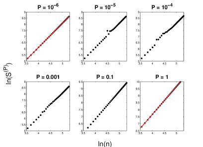
Figure 1: Log-log plot of von Neumann entropy, S, versus the scaled radius of the sphere ${\cal R}/a=n$, for $\tau=0$, $\epsilon=1$ and different values of coupling parameter $P$. The lattice size is $N=300$ and $50\leq n\leq 290$. The dots represent the numerical output and solid lines denote lines of best fit.

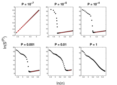
Figure 2: Log-log plot of von Neumann entropy, S, versus the scaled radius of the sphere ${\cal R}/a=n$, for $\tau=1$, $\epsilon=0$ and different values of coupling parameter $P$. The lattice size is $N=300$ and $100\leq n\leq 290$. $n_{c}$ for $P=10^{-5},10^{-4},10^{-3}$, respectively, are 139, 167 and 197.

(2) $\tau=1$, $\epsilon=0$: In Fig. (2), $\ln S^{(P)}$ versus $\ln({\cal R}/a)$ are plotted for different coupling parameter $P$, from which we infer the following: (i) For small $P$, as in the earlier case, entropy scales as area. (ii) As we increase $P$, above a critical value of $P$, say $P_{c}$ (here $P_{c}\sim 10^{-6}$) a new phase appears in the $\log-\log$ plots of entropy vs $n$. (iii) For a given $P>P_{c}$, scaling of $S^{(P)}$ changes drastically across some critical value of $n$, say $n_{c}$ (e.g. $n_{c}\sim 139$ for $P=10^{-5}$). For $n>n_{c}$, $S^{(P)}$ increases with $n$ and scales approximately close to area. However, for $n<n_{c}$, $S^{(P)}$ increases with decreasing $n$ i.e. $S^{(P)}\propto n^{-\alpha}$ ($\alpha>0$) (iv) With increasing $P$, $n_{c}$ increases. (V) Near $P=P_{c}$ transition is sharp. For $P>P_{c}$, the transition region is wider.

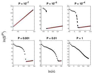
Figure 3: Log-log plot of von Neumann entropy, S, versus the scaled radius of the sphere ${\cal R}/a=n$, for $\tau=1$, $\epsilon=-1$ and different values of coupling parameter $P$. The lattice size is $N=300$ and $100\leq n\leq 290$. The dots represent the numerical output and solid lines denote lines of best fit.

(3) $\tau=1$, $\epsilon=-1$: Fig. (3) also shows similar cross-over of entanglement entropy as in the earlier case.

IV understanding the results

The above numerical results clearly indicate that higher derivative terms seem to drastically modify the vacuum structure, due to which the entropy jumps by few orders of magnitude close to the critical point, and throws up a large number of interesting questions. In the rest of this article, we address three key questions related to this new phenomena:

1. What universal feature the higher derivative terms have on the scaling of the entropy?

2. What causes the entropy to increase by couple of orders of magnitude at the cross-over?

3. Does the sharp jump indicate phase transition?

IV.1 Inverse scaling

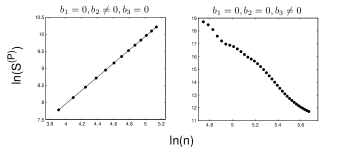
Figure 4: Log-Log plot of the entropy variation with only the 2nd order derivative term (left) and 3rd order derivative term (right) present in the Hamiltonian.

To go about answering question (I), let us set the dispersion relation for all $k$ modes to be $\omega^{2}=k^{4}/\kappa^{2}$ and $\omega^{2}=k^{6}/\kappa^{4}$. Repeating the earlier analysis, $\ln S^{(P)}$ vs $\log n$ in Fig. (4) shows that the fourth order derivative term leads to the usual area law while the sixth order derivative term shows inverse scaling i.e. entropy increases as we decrease $n$. Comparing Fig. (4) with $P=1$ plots in Fig. (2) show that increasing $P$ leads to the dominance of the higher-order derivative terms implying that the inverse scaling of entropy uniquely corresponds to the presence of higher (sixth) order derivative terms. The system has two distinct entropy profiles, the area law due to $(\nabla\phi)^{2}$ and inverse scaling due to $(\nabla^{3}\phi)^{2}$. Hence, for a particular coupling strength $P^{2}$, the two distinct entropy profiles appear at two regimes and a crossover happens at a $n_{c}$ that depends on $P$.

So, why the sixth-order derivative term leads to inverse scaling while the fourth-order derivative does not? One could plausibly get a better understanding of the phenomena if we look at the density of states and the two-point correlation function (Appendix C) for the three dispersion relations as given in Table (1). The density of states for the two dispersion relations ($k^{2}$ and $k^{4}$) increase with energy while for $\omega^{2}\propto k^{6}$, it is constant. The density of states is a kinematical quantity, the two point-function (See Appendix C) contains information about the quantum fluctuations. The two point function is scale-invariant for the dispersion relation $\omega^{2}\propto k^{6}$. We discuss the implications for condensed matter systems in conclusions.

Dispersion relation		Density of states		Two-point function
$\omega^{2}\propto k^{2}$		$D(\omega)d\omega\propto\omega^{2}d\omega$		$G^{+}\propto\frac{1}{r^{2}}$
$\omega^{2}\propto k^{4}$		$D(\omega)d\omega\propto\omega^{1/2}d\omega$		$G^{+}\propto\frac{1}{r}$
$\omega^{2}\propto k^{6}$		$D(\omega)d\omega\propto{\rm constant}~{}d\omega$		Scale-invariant

Table 1: Behavior of the density of states and two-point function for three dispersion relations: (i) $b_{1}\neq 0,b_{2}=b_{3}=0$, (ii) $b_{2}\neq 0,b_{1}=b_{3}=0$, (iii) $b_{3}\neq 0,b_{1}=b_{2}=0$.

IV.2 Critical mode

The plot of the distribution of entropy per partial wave $(2\ell+1)S_{\ell}$ versus $\ell$ can be used to answer question (II). Fig. (5) shows the entropy distribution for three values of $n$ for $\epsilon=0,\tau=1$ and $P=10^{-5}$ — $n=200$ (which falls in the positive slope region in Fig. 2), $n=137$ (which falls on the inverse scaling region in Fig. 2) and $n=110$. It can be seen that, for $n=200$, the contribution of large $\ell$ falls off rapidly implying that only lower partial waves $\ell$ contribute to the entropy. However, for $n=137$, at a critical mode ($\ell_{c}$), higher partial waves contribute significantly to entropy compared to lower $\ell$. For $n=110$ this happens at a lower $\ell_{c}$. This implies that, for a fixed $P$, as $n$ decreases, the turn around at which higher value of $\ell$ contribution to the entropy occurs earlier which in-turn leads to inverse scaling of entropy. This feature can be derived analytically by looking at $\ell\gg N$ limit of Hamiltonian (4):

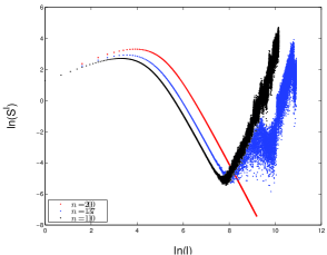
Figure 5: Log-Log plot of the entropy distribution per partial wave $S^{\ell}=(2\ell+1)S_{\ell}$ and $\ell$ for $n=200$, $137$ and $110$ for $P=10^{-5}$.

$$H\sim\frac{1}{2a}\sum_{i}\pi_{i}^{2}+\frac{l^{2}}{i^{2}}\left(1+\tau P^{2}~{}\frac{l^{4}}{i^{4}}\right)\phi_{i}^{2}+\mbox{higher-order terms}$$ (6)

In the region when the higher-derivative term dominates, we have,

$$\ell\geq P^{-1/2}{n}\,.$$ (7)

For a fixed $P<1$, as seen in Fig. (5), as $n$ increases the cross over occurs at larger $\ell$. In the case of $P\sim 1$, this implies that the cross over occurs much earlier leading to inverse scaling of entropy. For a detailed comparison of the entropy per mode among systems with different dispersion relations, see Appendix D. A qualitative understanding of excitation of higher modes (for $P>P_{c}$) can be understood using the quantum mechanical model of a particle in a box (see Appendix E).

IV.3 The cross-over

IV.3.1 Thermodynamic limit

To answer question (III) that the change in the ground state signals phase transition, we first calculate the entanglement entropy for different values of $N$ with $P=10^{-5},\tau=1,\epsilon=0$ and accuracy $10^{-5}$ (see Appendix F). Fig. 6 clearly shows the ratio $n_{c}/N$ remains almost constant with increasing $N$, implying that, the cross-over is indeed a quantum phase transition. It is important to note there is a no phase transition for $N=75$ indicating that $P_{c}$ decreases with increasing $N$.

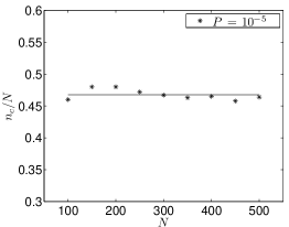
Figure 6: Variation of $\frac{n_{c}}{N}$ vs $N$ for $P=10^{-5}$.

IV.3.2 Scaling transformations

If $P_{c}$ is the quantum critical point, from the Wilsonian view point, at this point the (quantum) fluctuations occur at all length scales implying that action corresponding to Hamiltonian (2) or (4) is scale invariant. Under the scaling transformations $(e^{-l})$,

$$x_{i}^{\prime} = x~{}e^{-l};~{}~{}i=1,2,3$$ (8)

$$t^{\prime} = t~{}e^{-l},$$ (9)

$$\phi^{\prime} = \phi~{}e^{l},$$ (10)

$$\kappa^{\prime} = \kappa~{}e^{l}.$$ (11)

the action corresponding to (4) is invariant for any value of the effective coupling strength $P$ (since $a$ and $\kappa$ scales inversely). Also, the action corresponding to (2) is invariant and $\kappa$ flows to zero.

V Discussions

We have shown that linear, higher spatial derivative theories give rise to a new kind of quantum phase transition. The change in the scaling of entanglement entropy occurs due to two effects:

1. Kinematical: Change in the density of states from increasing to constant.

2. Dynamical: Excitation of larger $\ell$ modes compared to the canonical theory.

It is important to note that until now there is no fundamental understanding of the scaling of entanglement entropy with the density of states or the two-point correlation function. This work suggests a plausible link which will be explored in another work.

Recently, there has been interest in using entanglement as a probe to detect topological properties of many-body quantum states in two dimensional systems, like fractional quantum Hall effect 2006-Kiteav.Preskill-PRL ; 2008-Li.Haldane-PRL . Recently, it is found that Graphene shows an unconventional sequence of fractional quantum Hall states 2012-Feldman.etal-Science . Low-energy electronic states in Graphene are described by relativistic equation aka satisfying linear dispersion relation 2009-Neto.etal-RMP . The higher-order derivative term ($b_{2}\neq 0,b_{3}=0$) corresponds to Fermi gas has a constant density of state. Our work predicts that the above 2-D model will have an quantum phase transition. Currently, we are investigating the entanglement entropy to relate to the topological order.

It is usually expected that the higher derivative terms tame the UV divergences. In the case of two coupled harmonic oscillators Srednicki (1993), it is known that the entropy diverges when the interaction strength is large. The infinitesimal boundary tends to increase the interaction strength leading to the divergence of the entanglement entropy 1994-Bekenstein-Arx . As it is clear from our results, the divergence in the entanglement entropy can not be resolved by introducing higher derivative terms.

Our results have interesting implications to black-hole entropy: Numerical results for semi-classical black-holes have shown that close to $90\%$ of Hawking radiation is in s-wave 1976-Page-PRD . Our results show that this is the case for the linear dispersion relation (or large black-hole limit). However large $\ell$ modes contribute, when the non-linear dispersion relations are dominant. It is also important to note that earlier analyzes of Trans-Planckian effects on the Hawking radiation have been performed for $\ell=0$ Unruh (1995); Corley and Jacobson (1996). In the light of our analysis those calculations have to be revisited.

Due to Hawking radiation, the mass of the black-holes will decrease. As the size of the black-hole decreases, the curvature of the event-horizon increases and hence one need to include higher curvature terms Wald (1993); Jacobson and Myers (1993); Sen (2008); Kothawala and Padmanabhan (2009). Our analysis shows that as the size of the black-hole decreases, below a critical radius, the scaling of entropy changes instantaneously from area to inverse of area. It is interesting to look at the plausible implications of our result for the final stages of a microscopic black-hole.

Our results also seem to be related to causal dynamical triangulation approach of Ambjórn et al Ambjorn et al. (2005). There it has been shown that the continuum limit corresponds to the linear dispersion relation at large scales which in the UV limit changes to anisotropic scaling of space (with respect to time) corresponding to the dispersion relation $F(k)\propto k^{3}$. Recently, Horava Horava (2009) showed that gravity with dynamical critical exponent $m=3$ is perturbatively renormalizable (see also, Visser (2009)). Our analysis suggests that causal dynamical triangulation and Horava-Lifshitz model should also see a phase transition. These are under investigation.

Appendix A Entanglement entropy from density matrix

The Hamiltonian of a scalar field with modified dispersion relation, Eq. (2), in $(3+1)$-dimensional flat space, is given by:

$$H = \frac{1}{2}\int d^{3}x\left[\pi^{2}(x)+|\vec{\nabla}\varphi(\vec{x})|^{2}+\frac{\epsilon}{\kappa^{2}}(\vec{\nabla}^{2}\varphi(\vec{x}))^{2}+\frac{\tau}{\kappa^{4}}|\vec{\nabla}^{3}\varphi(\vec{x})|^{2}\right]~{}.$$ (12)

where $\kappa$ is the inverse length scale in the theory, $\epsilon=0,\pm 1$ and $\tau=0,1$.

Decomposing the field and its conjugate momentum in partial waves

$$\varphi(\vec{r})=\sum_{lm}\frac{\varphi_{lm}(r)}{r}~{}Y_{lm}(\theta,\phi)~{},~{}~{}\pi(\vec{r})=\sum_{lm}\frac{\pi_{lm}(r)}{r}~{}Y_{lm}(\theta,\phi)$$

yields:

$$H = \sum_{lm}H_{lm}$$ (13)

$$= \sum_{lm}\frac{1}{2}\int_{0}^{\infty}dr\left[\pi_{lm}^{2}(r)+r^{2}\left(\frac{\partial}{\partial r}\left(\frac{\varphi_{lm}(r)}{r}\right)\right)^{2}+\frac{l(l+1)}{r^{2}}\varphi_{lm}^{2}(r)+\frac{\epsilon}{\kappa^{2}}\left\{\frac{d^{2}\varphi}{dr^{2}}-\frac{l(l+1)}{r^{2}}\varphi_{lm}(r)\right\}^{2}\right.$$

$$\left.+\frac{\tau}{\kappa^{4}}\left\{\left(\frac{d^{3}\varphi}{dr^{3}}-\frac{1}{r}\frac{d^{2}\varphi}{dr^{2}}-\frac{l(l+1)}{r^{2}}\frac{d\varphi}{dr}+3l(l+1)\frac{\varphi}{r^{3}}\right)^{2}+\frac{l(l+1)}{r^{2}}\left(\frac{d^{2}\varphi}{dr^{2}}-l(l+1)\frac{\varphi}{r^{2}}\right)^{2}\right\}\right]$$

The discretizing scheme used in this work is different compared to that used by Srednicki Srednicki (1993). Srednicki’s mid-point discretization is not suited in the presence of higher-derivative terms. In this work, we have used central difference scheme, i.e.,

$$f^{\prime}(x) = \frac{f(x+1)-f(x-1)}{2\triangle x},$$

$$f^{\prime\prime}(x) = \frac{f(x+1)-2f(x)+f(x-1)}{(\triangle x)^{2}},$$

$$f^{\prime\prime\prime}(x) = \frac{f(x+2)-2f(x+1)+2f(x-1)-f(x-2)}{2(\triangle x)^{3}},$$ (14)

which is 2nd order accurate.

Eq. (13) can be written as the Hamiltonian of a set of $N$ coupled harmonic oscillators

$$H=\sum_{j}H_{j}=\frac{1}{2a}\sum_{i,j}^{N}\delta_{ij}\pi_{j}^{2}+\varphi_{j}\,K_{ij}\,\varphi_{i}$$ (15)

where the off-diagonal elements of the matrix $K_{ij}$ represent the interactions:

$$K_{ij} = \left[\frac{1}{i^{2}}+\frac{\epsilon}{a^{2}\kappa^{2}}+\frac{\tau}{a^{4}\kappa^{4}}\left\{F_{3}^{2}(2)+\frac{l(l+1)}{4}+\frac{1}{4}\right\}\right]\delta_{i1}\delta_{j1}-\frac{\tau}{4a^{4}\kappa^{4}}\left[\delta_{i2}\delta_{j2}+\delta_{i(N-1)}\delta_{j(N-1)}\right]$$ (16)

$$+\left[\frac{(N-1)^{2}}{4N^{2}}+\frac{\epsilon}{a^{2}\kappa^{2}}+\frac{\tau}{a^{4}\kappa^{4}}\left\{F_{1}^{2}(N-1)+\frac{l(l+1)}{(N-1)^{2}}+\frac{1}{4}\right\}\right]\delta_{iN}\delta_{jN}$$

$$+\left[\frac{(i^{2}+1)}{2i^{2}}+\frac{2\epsilon}{a^{2}\kappa^{2}}+\frac{\tau}{a^{4}\kappa^{4}}\left\{\frac{1}{2}+F_{2}^{2}(i-1)+F_{4}^{2}(i+1)+\frac{2(i^{2}+1)}{(i^{2}-1)^{2}}l(l+1)\right\}\right]\delta_{ij(i\neq 1,N)}$$

$$+\left[\frac{l(l+1)}{i^{2}}+\frac{\epsilon}{a^{2}\kappa^{2}}\left\{2+\frac{l(l+1)}{i^{2}}\right\}^{2}+\frac{\tau}{a^{4}\kappa^{4}}\left\{F_{2}^{2}(i)+\frac{l(l+1)}{i^{2}}F_{4}^{2}(i)\right\}\right]\delta_{ij}$$

$$+\left[-\frac{\epsilon}{a^{2}\kappa^{2}}\left\{4+l(l+1)\left(\frac{1}{j^{2}}+\frac{1}{(j+1)^{2}}\right)\right\}+\frac{\tau}{a^{4}\kappa^{4}}\left\{\frac{F_{1}(j-1)}{2}(1-\delta_{j1})+F_{1}(j)F_{2}(j)+\right.\right.$$

$$\left.\left.~{}~{}~{}~{}~{}~{}~{}~{}~{}~{}~{}~{}\frac{l(l+1)}{j^{2}}F_{4}(j)+F_{2}(j+1)F_{3}(j+1)+\frac{l(l+1)}{(j+1)^{2}}F_{4}(j+1)-\frac{F_{3}(j+2)}{2}(1-\delta_{iN})\right\}\right]\delta_{i,j+1}$$

$$+\left[-\frac{\epsilon}{a^{2}\kappa^{2}}\left\{4+l(l+1)\left(\frac{1}{i^{2}}+\frac{1}{(i+1)^{2}}\right)\right\}+\frac{\tau}{a^{4}\kappa^{4}}\left\{\frac{F_{1}(i-1)}{2}(1-\delta_{i1})+F_{1}(i)F_{2}(i)+\right.\right.$$

$$\left.\left.~{}~{}~{}~{}~{}~{}~{}~{}~{}~{}~{}~{}\frac{l(l+1)}{i^{2}}F_{4}(i)+F_{2}(i+1)F_{3}(i+1)+\frac{l(l+1)}{(i+1)^{2}}F_{4}(i+1)-\frac{F_{3}(i+2)}{2}(1-\delta_{jN})\right\}\right]\delta_{i,j-1}$$

$$-\left[\frac{(j+1)^{2}}{4j(j+2)}-\frac{\epsilon}{a^{2}\kappa^{2}}-\frac{\tau}{a^{4}\kappa^{4}}\left\{F_{1}(j+1)F_{3}(j+1)+\frac{l(l+1)}{(j+1)^{2}}+\frac{F_{2}(j)-F_{2}(j+2)}{2}\right\}\right]\delta_{i,j+2}$$

$$-\left[\frac{(i+1)^{2}}{4i(i+2)}-\frac{\epsilon}{a^{2}\kappa^{2}}-\frac{\tau}{a^{4}\kappa^{4}}\left\{F_{1}(i+1)F_{3}(i+1)+\frac{l(l+1)}{(i+1)^{2}}+\frac{F_{2}(i)-F_{2}(i+2)}{2}\right\}\right]\delta_{i,j-2}$$

$$+\frac{\tau}{a^{4}\kappa^{4}}\left[\left\{\frac{F_{3}(j+1)-F_{1}(j+2)}{2}\right\}\delta_{i,j+3}+\left\{\frac{F_{3}(i+1)-F_{1}(i+2)}{2}\right\}\delta_{i,j-3}-\frac{1}{4}(\delta_{i,j+4}+\delta_{i,j-4})\right]$$

where

$$F_{1}(i) = -1-\frac{1}{i}-\frac{l(l+1)}{2i^{2}},F_{2}(i)=\frac{2}{i}+\frac{3l(l+1)}{i^{3}},~{}~{}~{}~{}$$

$$F_{3}(i) = 1-\frac{1}{i}+\frac{l(l+1)}{2i^{2}},F_{4}(i)=-2-\frac{l(l+1)}{i^{2}}.$$ (17)

Note that $K_{ij}$ contains nearest-neighbor (nn), next to nn (nnn), next to nnn (nnnn) and next to nnnn (nnnnn) interaction terms due to the presence of higher derivative terms in (13). Schematically,

$$K_{ij}=\left(\begin{array}[]{lllllllll}{\times}&{\times}&{\times}&{\times}&{\times}&{}&{}&{}&{}\\ {\times}&{\times}&{\times}&{\times}&{\times}&{\times}&{}&{}&{}\\ {\times}&{\times}&{\times}&{\times}&{\times}&{\times}&{\times}&{}&{}\\ {\times}&{\times}&{\times}&{\times}&{\times}&{\times}&{\times}&{\times}&{}\\ {\times}&{\times}&{\times}&{\times}&{\times}&{\times}&{\times}&{\times}&{\times}\\ {}&{\times}&\times{}&{\times}&{\times}&{\times}&{\times}&{\times}&{\times}\\ {}&{}&{\times}&{\times}&{\times}&{\times}&{\times}&{\times}&\times{}\\ {}&{}&{}&{\times}&{\times}&{\times}&{\times}&{\times}&{\times}\\ {}&{}&{}&{}&{\times}&{\times}&{\times}&{\times}&{\times}\\ \end{array}\right)$$ (27)

A brief description of how to calculate entropy from the above Hamiltonian is the following. The density matrix, tracing over the first $n$ of $N$ oscillators ($r\equiv r_{n+1},\dots,r_{N}$), is given by:

$$\rho_{\rm reduced}=\int\prod_{i=1}^{n}~{}dr_{i}~{}\varphi(r_{1},\dots,r_{n};r_{n+1},\dots,r_{N})~{}\varphi^{\star}(r_{1},\dots,r_{n};r^{\prime}_{n+1},\dots,r_{N}^{\prime})$$ (28)

where $r$ and $r^{\prime}$ represent radial distances of the points, outside the horizon, from the center. The ground state is

$$\phi(r_{1},\dots,r_{N})=\prod_{i=1}^{N}N_{i}\exp(-\frac{1}{2}k_{Di}^{\frac{1}{2}}{\underline{r}}_{i}^{2}),~{}~{}~{}~{}~{}$$ (29)

(where $\underline{r}=Ur~{},~{}UKU^{T}=K_{D}~{}$ a diagonal matrix) the corresponding density matrix (28) can be evaluated exactly (the superscript $(0)$ signifies GS):

$$\rho_{\rm reduced}^{(0)}\sim\exp\left[-(r^{T}\gamma r+r^{\prime T}\gamma r^{\prime})/2+r^{T}\beta r\right]$$ (30)

where:

$$\Omega\sim K^{1/2}=\left(\begin{array}[]{ll}A&B\\ B^{T}&C\\ \end{array}\right)~{},~{}\beta=\frac{1}{2}B^{T}A^{-1}B~{},~{}\gamma=C-\beta~{}.$$ (31)

Note that $B$ and $\beta$ are non-zero if and only if there are interactions. The Gaussian nature of the above density matrix lends itself to a series of diagonalisations [$V\gamma V^{T}=$ diag, ${\bar{\beta}}\equiv\gamma_{D}^{-\frac{1}{2}}V\beta V^{T}\gamma_{D}^{-\frac{1}{2}}$, $W{\bar{\beta}}W^{T}=$ diag, $v_{i}\in v\equiv W^{T}(V\gamma V^{T})^{\frac{1}{2}}VT$], such that it reduces to a product of $(N-n)$, $2$-oscillator density matrices, in each of which one oscillator is traced over Srednicki (1993):

$$\rho^{(0)}_{{}_{\rm reduced}}\sim\prod_{i=1}^{N-n}\exp\left[-\frac{v_{i}^{2}+v_{i}^{\prime 2}}{2}+{\bar{\beta}}_{i}v_{i}v_{i}^{\prime}\right]~{}.$$ (32)

The corresponding entropy is given by:

$$S=\sum_{i=1}^{N-n}\left(-\ln[1-\xi_{i}]-\frac{\xi_{i}}{1-\xi_{i}}\ln\xi_{i}\right)~{}\left[\xi_{i}=\frac{{\bar{\beta}}_{i}}{1+\sqrt{1-{\bar{\beta}}_{i}^{2}}}\right]~{}.$$ (33)

Thus, for the full Hamiltonian $H=\sum_{lm}H_{lm}$, the entropy is:

$$S=\sum_{l=0}^{\infty}(2l+1)S_{l}$$ (34)

where the degeneracy factor $(2l+1)$ follows from spherical symmetry of the Hamiltonian. In practice, we will replace the upper bound of the sum in the above to a large value $l_{max}$. For the interaction matrix without any correction i.e. with $\epsilon=\tau=0$ in (16), the above entropy, computed numerically, turned out to be Bombelli et al. (1986); Srednicki (1993):

$$S=0.3(n+1/2)^{2}\equiv 0.3\left(\frac{R}{a}\right)^{2}~{}.$$ (35)

Appendix B Asymptotic analysis: Convergence of entropic contribution

For $l>>j$, the Hamiltonian can be written as

$$H\sim\frac{1}{2a}\sum_{i}\pi_{i}^{2}+\frac{l^{2}}{i^{2}}\left(1+\epsilon P~{}\frac{l^{2}}{i^{2}}+\tau P^{2}~{}\frac{l^{4}}{i^{4}}\right)\phi_{i}^{2}+\mbox{interaction/perturbative terms...}$$ (36)

In the case of $\epsilon=1$ and $\tau=0$ in the Hamiltonian (36), we get $\xi(P\rightarrow 0)=\frac{n^{4}}{64l^{4}}$ (where, $P=\frac{1}{a^{2}\kappa^{2}}$), where as the corresponding result of Srednicki was $\frac{n^{4}}{16l^{4}}$ Srednicki (1993) and $\xi(P\rightarrow 1)=\frac{n^{4}}{l^{4}}$.

In the case of $\epsilon=0$ and $\tau=1$, we get $\xi(P\rightarrow 0)=\frac{n^{4}}{l^{4}}$ and $\xi(P\rightarrow 1)=\frac{17n^{4}}{16l^{4}}+\frac{n^{6}}{l^{6}}+\frac{n^{12}}{l^{12}}$. These values confirm that the entropy converges for large $l$ and justifies the use of an upper cutoff $l_{max}$ for numerical estimation.

Appendix C Calculation of correlation function

The two point correlation function of the fields also provide information about structure of the scalar field from the linear to non-linear dispersion relations. The (equal time) two-point correlation function or the Wightman function is given by

$$G^{+}(x^{\mu},y^{\mu}) = \int\frac{d^{3}k}{(2\pi)^{3}}\frac{\exp[i\vec{k}.(\vec{x}-\vec{y})]}{2\omega}$$ (37)

$$= \frac{1}{4\pi^{2}r}\int_{0}^{\infty}\frac{k}{\omega}~{}\sin(kr)~{}dk$$

where $r=|{\vec{x}}-{\vec{y}}|$. Eq. (37) can be rewritten for a general dispersion relation $\omega=k^{m}$ and with substitution $kr=\alpha$ as

$$G^{+}(x^{\mu},y^{\mu})=\frac{r^{m-3}}{4\pi^{2}}\int_{0}^{\infty}\frac{\sin\alpha}{\alpha^{m-1}}~{}d\alpha$$ (38)

Note that for linear ($m=1$) and quadratic ($m=2$) dispersion models correlation decays with increasing distance which explains the area-law behavior of the entropy. Interestingly when the third order correction ($m=3$) is dominant, the correlation function essentially becomes scale invariant.

Appendix D Entropy per partial wave for different dispersion models

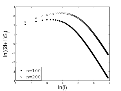
Figure 7: Entropy distribution per partial wave $(2\ell+1)S_{\ell}$ and $\ell$, in linear dispersive system ($m=1$), for $n=200$ and $n=100$.

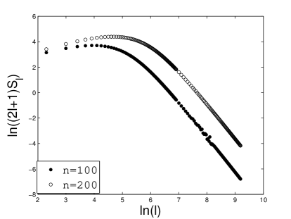
Figure 8: Entropy distribution per partial wave $(2\ell+1)S_{\ell}$ and $\ell$, in quadratic dispersive system ($m=2$), for $n=200$ and $n=100$.

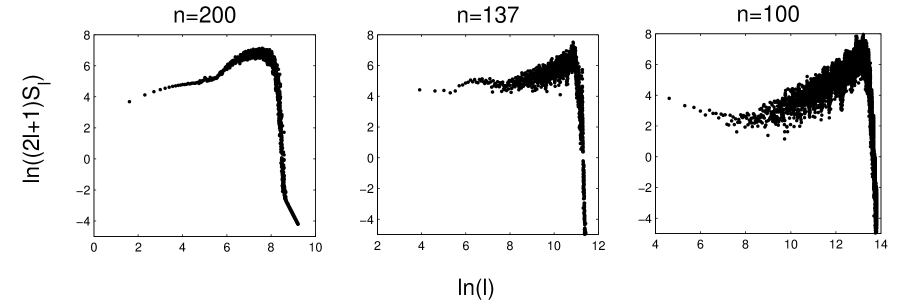
Figure 9: Entropy distribution per partial wave $(2\ell+1)S_{\ell}$ and $\ell$, in cubic dispersive system ($m=3$), for $n=200$, $n=137$ and $n=100$.

Fig. 8 and Fig. 8 shows that in linear and quadratic dispersive theories, with decreasing $n$, entropy per partial wave decreases. On the other hand for cubic dispersion theory exactly opposite behavior is found (see Fig. 9).

Appendix E Particle in a box model

The Schrödinger equation corresponding to a general non-linear dispersion model is:

$$\frac{d^{2m}\psi}{dx^{2m}}+{\cal E}\psi=0\qquad\quad{\cal E}=E\kappa_{{}_{P}}^{2(m-1)}.$$ (39)

The most general solution is given by

$$\psi(x)=\sum_{j=1}^{2m}C_{j}\exp[(-1)^{\frac{2j-1}{2m}}{\cal E}^{\frac{1}{2m}}x]\,,$$ (40)

where $C_{j}$’s are constants to be determined by the boundary conditions. In particular, for $m=1$, $2$ and $3$, the general solution is given by:

$$\psi_{m=1} = c_{1}\cos({\cal E}^{\frac{1}{2}}x)+c_{2}\sin({\cal E}^{\frac{1}{2}}x)$$ (41)

$$\psi_{m=2} = \exp\left(\frac{{\cal E}^{\frac{1}{4}}x}{\sqrt{2}}\right)\left[c_{1}\cos\left(\frac{{\cal E}^{\frac{1}{4}}x}{\sqrt{2}}\right)+c_{2}\sin\left(\frac{{\cal E}^{\frac{1}{4}}x}{\sqrt{2}}\right)\right]$$ (42)

$$+\exp\left(-\frac{{\cal E}^{\frac{1}{4}}x}{\sqrt{2}}\right)\left[c_{3}\cos\left(\frac{{\cal E}^{\frac{1}{4}}x}{\sqrt{2}}\right)+c_{4}\sin\left(\frac{{\cal E}^{\frac{1}{4}}x}{\sqrt{2}}\right)\right]$$

$$\psi_{m=3} = \exp\left(\frac{{\sqrt{3}\cal E}^{\frac{1}{6}}x}{2}\right)\left[c_{1}\cos\left(\frac{{\cal E}^{\frac{1}{6}}x}{2}\right)+c_{2}\sin\left(\frac{{\cal E}^{\frac{1}{6}}x}{2}\right)\right]$$ (43)

$$+\exp\left(-\frac{\sqrt{3}{\cal E}^{\frac{1}{6}}x}{2}\right)\left[c_{3}\cos\left(\frac{{\cal E}^{\frac{1}{6}}x}{2}\right)+c_{4}\sin\left(\frac{{\cal E}^{\frac{1}{6}}x}{2}\right)\right]$$

$$+c_{5}\cos\left({\cal E}^{\frac{1}{6}}x\right)+c_{6}\sin\left({\cal E}^{\frac{1}{6}}x\right)$$

For a particle in a box model, only exponentially growing and decaying solutions exist for even $m$, while for odd $m$ one has stationary solutions [$\sim\sin({\cal E}^{\frac{1}{2m}}x)$]. With the appropriate boundary conditions at $x=0$ and $L$, one finds the energy eigenvalues are $E_{\nu}$:

$$E_{\nu}\sim\left(\frac{\nu\pi}{L}\kappa^{\frac{1-m}{m}}\right)^{2m}\qquad\nu=1,2,..$$ (44)

which leads to:

$$\frac{\mbox{\small Ground state energy eigenvalue for $m=1$}}{\mbox{\small Ground state energy eigenvalue for $m>1$}}=\left[\frac{L\kappa}{\pi}\right]^{2(m-1)}$$ (45)

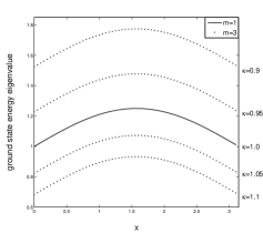
Figure 10: Energy eigenvalues for $m=1$ and $3$, $L=\pi$ and varying $\kappa$.

For $m>1$, with decreasing $\kappa$, the ground state energy eigenvalue of the system increases. Fig. (10) shows that at $\kappa=\pi/L$, it crosses the ground state energy eigenvalue for the system satisfying linear dispersion relation ($m=1$) and becomes more than that for $\kappa<\pi/L$.

Eq. (45) implies that, for $\kappa<\pi/L$, the ground state energy eigenvalue in the non-linear dispersion theory is higher compared to that of linear dispersion theory. As in the field theory model, where there is a cross-over from the linear to non-linear regime, with increasing $P$ (or decreasing $\kappa$), for $P>P_{c}$, the system needs to readjust in such a way that the ground state energy of the system increases. In other words, the cross-over of the dispersion relation catalyzes larger population of higher energy quantum states compared to low-energy states.

Appendix F Transition in the thermodynamic limit

Fig. 11 shows that, for fixed $P$ with increasing $N$ the transition happens approximately at the same $n_{c}/N$ though it looses it’s sharpness. The inverse scaling does not appear for $N=75$ implying that $P_{c}$ decreases with increasing $N$.

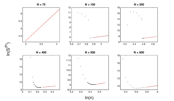
Figure 11: Entropy profile for $P=10^{-5}$ with different system size $N$.

References

- Horodecki et al. (2009) R. Horodecki, P. Horodecki, M. Horodecki, and K. Horodecki, Rev. Mod. Phys. 81, 865 (2009).
- Eisert et al. (2010) J. Eisert, M. Cramer, and M. B. Plenio, Rev. Mod. Phys. 82, 277 (2010), eprint 0808.3773.
- Bombelli et al. (1986) L. Bombelli, R. K. Koul, J.-H. Lee, and R. D. Sorkin, Phys. Rev. D34, 373 (1986).
- Srednicki (1993) M. Srednicki, Phys. Rev. Lett. 71, 666 (1993).
- Das et al. (2008) S. Das, S. Shankaranarayanan, and S. Sur, Phys. Rev. D77, 064013 (2008), eprint 0705.2070.
- Sondhi et al. (1997) S. L. Sondhi, S. M. Girvin, J. P. Carini, and D. Shahar, Rev. Mod. Phys. 69, 315 (1997).
- Sachdev (2001) S. Sachdev, Quantum phase transitions, (Cambridge University Press, 2001), ISBN 9780521004541.
- Carr (2011) L. Carr, Understanding quantum phase transitions, (CRC Press, 2011), ISBN 9781439802519.
- Osterloh et al. (2002) A. Osterloh, L. Amico, G. Falci, and R. Fazio, Nature 416, 608 (2002), eprint arXiv:quant-ph/0202029.
- Osborne and Nielsen (2002) T. J. Osborne and M. A. Nielsen, Phys. Rev. A 66, 032110 (2002), eprint arXiv:quant-ph/0202162.
- Wu et al. (2004) L.-A. Wu, M. S. Sarandy, and D. A. Lidar, Phys. Rev. Lett. 93, 250404 (2004), eprint arXiv:quant-ph/0407056.
- Rieper et al. (2010) E. Rieper, J. Anders, and V. Vedral, New J. Phys. 12, 025017 (2010), eprint 0908.0636.
- (13) P. W. Anderson, Science 177, 393-396 (1972)
- Toledano (1987) J. C. Toledano, and P. Toledano, The Landau Theory of Phase Transitions, (World Scientific, 1987).
- Hornreich et al. (1975) R. M Honreich, M. Luban, and S. Shritman, Phys. Rev. Lett. 35, 1678 (1975).
- Unruh (1995) W. G. Unruh, Phys. Rev. D51, 2827 (1995).
- Corley and Jacobson (1996) S. Corley and T. Jacobson, Phys. Rev. D54, 1568 (1996).
- Padmanabhan (1999) T. Padmanabhan, Phys. Rev. D59, 124012 (1999).
- Visser (2009) M. Visser, Phys. Rev. D80, 025011 (2009), eprint 0902.0590.
- Lookman et al. (2003) T. Lookman, S. R. Shenoy, K. O. Rasmussen, A. Saxena, and A. R. Bishop, Phys. Rev. B. 67, 024114 (2003).
- (21) A. Kitaev and J. Preskill, Phys. Rev. Letts. 96, 110404 (2006).
- (22) H. Li and F. D. M. Haldane, Phys. Rev. Letts. 101, 010504 (2008).
- (23) B. Feldman, B. Krauss, J. Smet and A. Yacoby, Science, 337, 1196-1199 (2012).
- (24) A. H. Castro Neto, F. Guinea, N. M. R. Peres, K. S. Novoselov, and A. K. Geim Rev. Mod. Phys. 81, 109 (2009)
- (25) J. D. Bekenstein, gr-qc/9409015.
- (26) D. N. Page, Phys. Rev. D 13, 198 (1976).
- Wald (1993) R. Wald, Phys. Rev. D48, R3427 (1993), eprint gr-qc/9307038.
- Jacobson and Myers (1993) T. Jacobson and R. C. Myers, Phys. Rev. Lett. 70, 3684 (1993), eprint hep-th/9305016.
- Sen (2008) A. Sen, Gen. Rel. Grav. 40, 2249 (2008), eprint 0708.1270.
- Kothawala and Padmanabhan (2009) D. Kothawala and T. Padmanabhan, Phys. Rev. D79, 104020 (2009), eprint 0904.0215.
- Ambjorn et al. (2005) J. Ambjorn, J. Jurkiewicz, R. Loll, Phys. Rev. Lett. 95, 171301 (2005).
- Horava (2009) P. Horava, Phys. Rev. Lett. 180, 161301 (2009).