Sensitivity to Dark Energy candidates by searching for four-wave mixing of high-intensity lasers in the vacuum

Abstract

Theoretical challenges to understand Dark Matter and Dark Energy suggest the existence of low-mass and weakly coupling fields in the universe. The quasi-parallel photon-photon collision system (QPS) can provide chances to probe the resonant production of these light dark fields and the induced decay by the coherent nature of laser fields simultaneously. By focusing high-intensity lasers with different colors in the vacuum, new colors emerge as the signature of the interaction. Because four photons in the initial and final states interplay via the dark field exchange, this process is analogous to four-wave mixing in quantum optics, where the frequency sum and difference among the incident three waves generate the fourth wave with a new frequency via the nonlinear property of crystals. The interaction rate of the four-wave mixing process has the cubic dependence on the intensity of each wave. Therefore, if high-intensity laser fields are given, the sensitivity to the weakly coupling of dark fields to photons rapidly increases over the wide mass range below sub-eV. Based on the experimentally measurable photon energies and the linear polarization states, we formulate the relation between the accessible mass-coupling domains and the high-intensity laser parameters, where the effects of the finite spectrum width of pulse lasers are taken into account. The expected sensitivity suggests that we have a potential to explore interactions at the Super-Planckian coupling strength in the sub-eV mass range, if the cutting-edge laser technologies are properly combined.

I Introduction

Ordinary matter occupies only $\sim 4$% of the total energy density of the universe. The remaining energies are supposed to be occupied by Dark Matter (DM) $\sim 23$% and Dark Energy (DE) $\sim 73$% WMAP . In addition to the astronomical observations, directly probing these dark components in terrestrial laboratory experiments has crucial roles to provide different insights into the true characters of the universe or the structure of the vacuum.

Light (pseudo)scalar fields are now indispensable theoretical tools to try to interpret the cosmological constant $\Lambda$ based on the DE scenario DEreview . In reduced Planckian units with $c=\hbar=M_{P}(=(8\pi G)^{-1/2}\sim 10^{27}{\rm eV})=1$, the observed $\Lambda\sim 10^{-120}$ is extremely small compared to the theoretically natural scale $\Lambda\sim 1$. There is a variety of theoretical models in the market. In order for a DE model to be falsifiable by laboratory experiments, we clarify following minimum requirements on the model:

• solves the fine-tuning problem; how to realize such an extremely small $\Lambda$,

• solves the coincidence problem; why the energy density coincides with the matter density only at once at present so accidentally among the long history of the universe,

• predicts the field-matter coupling strength, the mass scale of the exchanged field, and the measurable dynamical effect, e.g., the force-range.

For instance, quintessence approaches DEreview are designed to resolve the fine-tuning and coincidence problems by introducing decaying behavior of $\Lambda$ based on a potential of a scalar field. However, the potential forms are rather phenomenologically introduced. In the similar course, the scalar-tensor theory with $\Lambda$ ($STT\Lambda$) STTL , on the other hand, is grounded upon the conformal transformation and the frame of observations, which gives several testable predictions. Therefore, $STT\Lambda$ is one of the DE models satisfying the above requirements simultaneously. The most significant prediction of $STT\Lambda$ is the decaying behavior of $\Lambda\propto t^{-2}$ as a function of time $t$. The present age of the universe is $t_{0}\sim 1.37\times 10^{10}$ year corresponding to $t_{0}\sim 10^{60.2}$ in reduced Planckian units. Thus, the observed $\Lambda$ is naturally understood by the overall decaying behavior, though expecting short-term fluctuations from the dominant behavior STTtrap . The decaying behavior depends on the conformal frame on which our observations are based. For example, redshift measurements relevant to DE is implicitly based on the common atomic clock between distant points, i.e., on the common elementary particle masses. In order to realize constancy of particle masses, a consistent conformal frame must be favored on which the gravitational constant $G$ looks constant, the expansion rate of the universe is consistent with the observation, and $\Lambda$ decays as $t^{-2}$ by keeping particle masses constant FujiiShort . The choice of a conformal frame unavoidably associates a massless Nambu-Goldstone (NG) boson, because it breaks scale invariance (global conformal symmetry), which is also known as dilaton. In contrast to the well-known Brans-Dicke model BD , a kind of scalar-tensor theories, the requirement of constancy of particle masses results in coupling of the scalar field with matter, i.e., violation of Weak Equivalence Principle only via quantum anomaly coupling STTL . Due to this coupling to matter fields, $STT\Lambda$ uniquely predicts an extremely low-mass scalar field as a pseudo NG boson via the explicit symmetry breaking by the quantum loop effect in the self-energy. This is similar to a massive pion as a theoretical descendant of an originally massless NG pseudoscalar boson associated with chiral symmetry. The scalar field couples with other matter fields basically as weakly as gravity. The mass scale $m_{\phi}$ based on the simple one-loop diagram in which the light quarks and leptons with a typical mass $m_{\rm q}\sim{\rm MeV}$ couple to the scalar field with the gravitational coupling with the strength $\sim M_{\rm P}^{-1}$ is given by

$$m_{\phi}^{2}\sim\frac{m_{\rm q}^{2}M_{\rm ssb}^{2}}{M_{\rm P}^{2}}\sim(10^{-9}{\rm eV})^{2},$$ (1)

where the effective cutoff coming from the super-symmetry-breaking mass-scale $M_{\rm ssb}\sim{\rm TeV}$ is assumed, though allowing a latitude of several orders of magnitude, if $M_{\rm ssb}$ is higher than the conventional TeV scale STTL . We note that the uncertainty on the mass range in the DE scenarios is quite large. Quintessence-based scenarios typically argue that the mass is determined from the second derivative of the assumed almost flat potential resulting in $m\sim 10^{-33}$ eV . On the other hand, $\Lambda\sim$ (meV)⁴ in natural units intuitively leads models based on the particle pictureQA ; Chameleon ; deVega assuming the mass scale in the meV range via rather complicated assumptions. For example, the axion inspired models QA share the similarity to $STT\Lambda$ by introducing the concept of pseudo NG boson driven by the two dominant scales, $M_{P}$ and a scale of the assumed symmetry breaking at a lower energy than $M_{P}$  .

The finite mass of the scalar field in $STT\Lambda$ causes non-Newtonian force YFujii via the Yukawa potential, a.k.a. fifth force. The inverse of Eq.(1) gives a finite range corresponding to $\sim 100$ m of the force mediated by the exchange of a quantum $\phi$ between local objects. This is an entirely different aspect from its way of a cosmological fluid in accelerating the universe. The force-range has not been explicit in the other theoretical models. This unique aspect triggered the past experimental efforts to measure deviations from the Newtonian potential between massive test bodies FifthExp in different contexts from DE at that time. These measurements, however, accompany large systematic uncertainties due to the uncontrollable macroscopic probes. As an alternative approach, we have proposed to utilize the nature of high-intensity laser fields toward laboratory search for the scalar field predicted by $STT\Lambda$ DEptp as an ultimate goal of laboratory experiments.

Furthermore, low-mass and weakly coupling fields are also predicted in the contexts of particle physics with the solid foundation. For example, axion, the pseudoscalar field is proposed as a NG boson associated with the global Peccei and Quinn symmetry breaking PQ to naturally maintain the $CP$ conserving nature of the QCD Lagrangian. Axion and invisible axion-like fields have been intensively investigated by astrophysical objects as well as laboratory experiments AxionReview . Some of them may become cold dark matter candidates, if the mass and the coupling to matter are within the proper range. Such fields may also leave observational isocurvature fluctuations, if the symmetry breaking occurs during the inflation phase of the early universe CDM . If we can anticipate that the experimental sensitivity reaches the gravitational coupling strength, the detection of such cold matter candidates with much stronger couplings to matter naturally comes into view as the preliminary step toward the ultimate goal.

We, therefore, generalized the principle of the measurement to search for both scalar and pseudoscalar fields in a model independent way as much as possible DEapb . As amplitudes of laser fields are increased, we can improve the sensitivity to weakly coupling low-mass fields predicted by any types of theories, as long as the coupling to photons is expected. The proposed method can be regarded as a kind of particle colliders attempting to produce extremely light resonance states. The mass range of interest is, however, for instance, much lower than that of Higgs-like boson produced at Large Hadron Collider (LHC) by more than ten orders of magnitude. In the proposed method, following two key ingredients to enhance the sensitivity are included.

The first ingredient is the introduction of the quasi-parallel photon-photon collision system (QPS) as illustrated in Fig.1. This is considered to realize the center-of-mass system (CMS) energy as low as possible between colliding two laser photons for the production of a low-mass field as a resonance state without lowering the incident photon energy below optical frequency. The head-on collision in CMS corresponds to the case $\vartheta=\pi/2$ in Fig.3. The quasi-parallel system can be obtained by introducing a Lorentz boost of the head-on collision into the perpendicular direction with respect to the incident direction in CMS. The CMS energy $E_{cms}$ is then expressed as $E_{cms}=2\omega\sin\vartheta$ with the incident energy of photon $\omega$. If a small $\vartheta$ is realized in the laboratory frame, it provides an extremely low CMS energy. This is the essence of the introduction of QPS. Moreover, fortunately thanks to the strong Lorentz boost, QPS provides frequency-shifted photons as the decay product of the resonance state, which becomes a distinct observational signal as the indication of the interaction. However, as we discuss in the next section briefly, the resonance point cannot be directly captured due to the extremely narrow resonance by the weakly coupling compared with the momentum uncertainty of incident photons in QPS. This situation requires an averaging process of the cross section over the possible uncertainty of the CMS energy in QPS. By this averaging, the non-negligible effect of the narrow resonance is enhanced by the square of the inverse coupling compared with the case where no resonance state is contained. If the coupling to two photons is proportional to $1/M_{P}$, the huge enhancement by $M^{2}_{P}$ is expected.

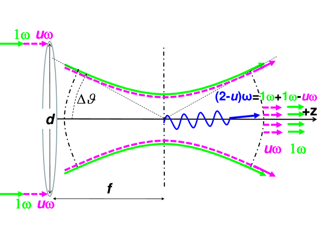
Figure 1: Quasi parallel colliding system (QPS) between two incident photons out of a focused laser beam with the focal length $f$, the beam diameter $d$, and the upper range of incident angles $\Delta\vartheta$ determined by geometric optics. The signature $(2-u)\omega$ is produced via the four-wave mixing process, $1\omega+1\omega\rightarrow(2-u)\omega+u\omega$ with $0<u<1$ by mixing two waves with different frequencies $1\omega$ and $u\omega$ in advance at the incidence.

The second ingredient is the enhancement by the coherent nature of laser fields Glauber or the degenerate nature of Bosonic particles as illustrated in Fig.2. This Bosonic nature of the laser beam is fundamentally important, because we can induce the decay of the produced resonance state into a specific momentum space as the principle of the laser amplification itself utilizes that nature. We propose to use different frequencies between the production and inducing laser beams, respectively. As shown in the figure, the exchange of the low-mass field is interpreted as the four-wave mixing process where three waves (the two waves are degenerate and the one wave has a different frequency from the degenerate waves) are combined and the forth wave emerges with a new frequency not included in the originally mixed laser waves. This four-wave mixing process is well-known in quantum optics FWM . The process is already applied to generate a different color wave from those of incident laser beams via the nonlinear atomic processes of crystals. In other words, the proposed method is as if the atomic nonlinear process is replaced by the nonlinear process of the vacuum via the low-mass field exchange. In the context of the QED interaction, a similar approach is discussed QEDchi3 and the experimental setups are proposed QEDfwm . The upper limit of the photon-photon cross section is provided by this method QEDlimit . Since each of the two photons at the first vertex annihilates into the coherent state with $1\omega$, while another photon at the second vertex is created from the coherent state with $u\omega$ with $0<u<1$, the interaction rate to observe $(2-u)\omega$ frequency is eventually enhanced by a factor of $(\sqrt{N_{1\omega}}\sqrt{N_{1\omega}}\sqrt{N_{u\omega}})^{2}$ DEptp , where $N$ indicates the average number of laser photons with individual frequency specified by the subscripts. This cubic dependence of the interaction rate motivates us to make the laser energy per pulse as large as possible.

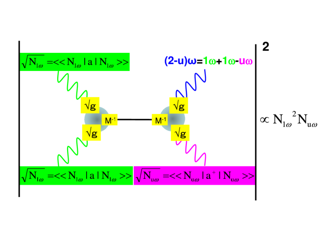
Figure 2: Four-wave mixing process in the vacuum. The state $|N\rangle\rangle\equiv e^{-N/2}\sum_{n=0}^{\infty}\frac{N^{n/2}}{\sqrt{n!}}|n\rangle$ with $|n\rangle$ being the degenerate state of $n$ photons refers to the coherent states Glauber with the average number of photons $N$. The coherent states are distinguished with photon frequencies specified by the individual subscripts. The probability to create $(2-u)\omega$ with $0<u<1$ is expected to have the cubic dependence on $N$, because expectation values of creation and annihilation operators associated with the individual photon legs become $\sqrt{N}$ in the scattering amplitude DEptp . The effective dark field - two photon coupling $gM^{-1}$ for each vertex corresponds to the coupling in the effective interaction Lagrangian defined in Eq.(2).

In this paper, we extend the formula discussed in the recent works  DEptp ; DEapb and then provide the prescription to relate the accessible mass-coupling domains by taking an essence of realistic experimental constraint such as a state of the multi-frequency mode with a finite frequency bandwidth and the effect of the specification of linear polarization states, when we attempt to apply this method to experiments based on pulse lasers. The expected sensitivity to the low-mass and weakly coupling fields is provided for anticipated high-intensity laser fields available at laboratories over the world at present and in the near future ISMD2011 . The result suggests that the state-of-the-art technology may provide access to interactions with gravitational coupling strength and even beyond it (Super-Planckian coupling) for relatively higher mass ranges in the sub-eV mass domain. We emphasize that the proposed approach is a kind of Bosonic collider. The commonality and the distinctions from the Fermionic collider, for example LHC, is discussed as a concluding remark.

II Formulae to relate sensitivity and laser parameters

Let us briefly review the necessary parts for the extension in order to consider the effects of the finite spectrum widths and the specification of linear polarization states of laser fields.

The effective interaction Lagrangian between two photons and an unknown low-mass scalar or pseudoscalar fields $\phi$ or $\sigma$ are generalized as follows, respectively

$$-L_{\phi}=gM^{-1}\frac{1}{4}F_{\mu\nu}F^{\mu\nu}\phi\quad{\mbox{o}r}\quad-L_{\sigma}=gM^{-1}\frac{1}{4}F_{\mu\nu}\tilde{F}^{\mu\nu}\sigma,$$ (2)

where $M$ has the dimension of mass while $g$ being a dimensionless constant. Depending on the allowed polarization combinations of two photons coupling to the dark fields, we can argue whether they are scalar-type or pseudoscalar-type in general as we see in Appendix in detail.

We summarize the notations and kinematics based on the equation (2.1)-(2.3) of  DEptp . We label momenta to four photons as illustrated in Fig.3, where the incident angle $\vartheta$ is assumed to be symmetric around the $z$-axis, because we assume the symmetric focusing as illustrated in Fig.1. For later convenience, we introduce an arbitrary number $u$ with $0<u<1$ to re-define momenta of the final state photons as $\omega_{4}\equiv u\omega$ and $\omega_{3}\equiv(2-u)\omega$. By this definition, we require $0<\omega_{4}<\omega_{3}<2\omega$. We consider the case where we measure $\omega_{3}$ with the specified polarization state as the signature of the interaction. With these definitions, energy-momentum conservation in DEptp is re-expressed as

$$(2-u)\omega+u\omega=2\omega$$ (3)

$$(2-u)\omega\cos\theta_{3}+u\omega\cos\theta_{4}=2\omega\cos\vartheta$$ (4)

$$(2-u)\omega\sin\theta_{3}=u\omega\sin\theta_{4}.$$ (5)

From these, we also derive the following relation

$$\frac{\sin\theta_{3}}{\sin\theta_{4}}=\frac{\sin^{2}\vartheta}{1-2\cos\vartheta\cos\theta_{4}+\cos^{2}\vartheta},$$ (6)

and

$$\omega_{3}=(2-u)\omega=\frac{\omega\sin^{2}\vartheta}{1-\cos\vartheta\cos\theta_{3}}.$$ (7)

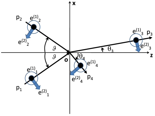
Figure 3: Definitions of kinematical variables DEptp . The exact definitions of the photon momenta and the polarization vectors can be found in Appendix.

From (2.5) of DEptp , the differential cross section per solid angle of $p_{3}$ is expressed as

$$\frac{d\sigma}{d\Omega_{3}}=\left(\frac{1}{8\pi\omega}\right)^{2}\sin^{-4}\vartheta\left(\frac{\omega_{3}}{2\omega}\right)^{2}|{\cal M}_{S}|^{2},$$ (8)

where $|{\cal M}_{S}|^{2}$ is the square of the invariant scattering amplitude including the resonance state in the $s$-channel with a sequence of four-photon polarization states $S=\beta_{1}\beta_{2}\beta_{3}\beta_{4}$ specified by the polarization vectors $\vec{e_{i}}^{(\beta_{i})}$ with $i=1,2,3,4$ for the photon labels, whereas $\beta=1,2$ are the kind of the linear polarization as indicated in Fig.3. As we discuss how to evaluate the amplitudes in Appendix, $S=1111,2222,1122,2211$ and $S=1212,1221,2112,2121$ give the non-vanishing invariant amplitudes for scalar and pseudoscalar exchanges, respectively.

The enhancement by the inducing laser field labeled as $p_{4}$ is limited to the intrinsic spectrum width of the inducing laser energy due to energy-momentum conservation, which is defined as

$$\delta\omega_{4}\equiv\overline{\omega_{4}}-\underline{\omega_{4}}=(\delta u)\omega,$$ (9)

where $\delta u\equiv\overline{u}-\underline{u}$ with $0<\overline{u}<1$, $0<\underline{u}<1$ and $\overline{u}>\underline{u}$. The overline and underlines attached to the simple variables indicate the allowed maximum and minimum values, respectively. This notation is used repeatedly, unless confusion occurs. The spectrum width of $\omega_{3}$ is simultaneously constrained to

$$\delta\omega_{3}\equiv\overline{\omega_{3}}-\underline{\omega_{3}}=(2-\underline{u})\omega-(2-\overline{u})\omega=(\delta u)\omega$$ (10)

due to energy-momentum conservation as well. This indicates that the energy range to detect $\omega_{3}$ must be consistent with $\delta\omega_{4}$ in order to get the full enhancement factor by the inducing laser.

By assuming that $\delta\omega_{3}=\delta\omega_{4}$ is realized in an experimental setup, let us now calculate the cross section integrated over $\delta\omega_{3}$ as a function of the spectrum width parameter $(\overline{u},\underline{u})$. Eventually $\delta\omega_{3}$ gives the range of the integral via the range of scattering angle $\theta_{3}$. The integrated cross section over the range of $\theta_{3}$ from $\underline{\theta_{3}}$ to $\overline{\theta_{3}}$ is expressed as

$$\overline{\sigma}=\frac{{\cal F}_{S}\overline{|{\cal M}_{S}|^{2}}}{(8\pi\omega)^{2}\sin^{4}\vartheta}\int_{\underline{\theta_{3}}}^{\overline{\theta_{3}}}\left(\frac{\omega_{3}}{2\omega}\right)^{2}\sin\theta_{3}d\theta_{3}\equiv\frac{{\cal F}_{S}\overline{|{\cal M}_{S}|^{2}}}{(8\pi\omega)^{2}}{\cal I},$$ (11)

by defining

$${\cal I}\equiv\frac{1}{\sin^{4}\vartheta}\int_{\underline{\theta_{3}}}^{\overline{\theta_{3}}}\left(\frac{\omega_{3}}{2\omega}\right)^{2}\sin\theta_{3}d\theta_{3}=\left[\frac{1}{4\cos\vartheta(1-\cos\theta_{3}\cos\vartheta)}\right]^{\underline{\theta_{3}}}_{\overline{\theta_{3}}},$$ (12)

where $\overline{|{\cal M}_{S}|^{2}}$ denotes the averaged $|{\cal M}_{S}|^{2}$ over possible uncertainty on the incident angle $\vartheta$ as we briefly discuss below, and ${\cal F_{S}}$ corresponds to the integral over the azimuthal degree of freedom depending on the specification of photon polarizations in the initial and final states. If the scattering amplitude has the axial symmetry around the $z$-axis in Fig.3, ${\cal F_{S}}$ simply corresponds to $2\pi$. As we summarize in Appendix, however, the axial asymmetries actually appear depending on $S$ specified by experimental conditions, which result in deviations from $2\pi$. We then convert the variable $\cos\theta_{3}$ to $u$ based on Eq.(7) from which we express

$$\cos\theta_{3}=\frac{1}{\cos\vartheta}\left(1-\frac{\omega}{\omega_{3}}\sin^{2}\vartheta\right)\sim 1+\frac{1}{2}\vartheta^{2}\left(1-\frac{2\omega}{\omega_{3}}\right)=1+\frac{1}{2}\vartheta^{2}\left(1-\frac{2}{2-u}\right),$$ (13)

where terms of the order higher than $\vartheta^{2}$ are dropped when applied to the low-mass resonance. From this, Eq.(12) is also approximated as

$${\cal I}\sim\frac{\delta u}{4\vartheta^{2}}.$$ (14)

We now consider the scattering amplitudes only for the case when low-mass fields are exchanged via the resonance states in the s-channel. The resonance decay rate of the low-mass field with the mass $m$ into two photons is expressed as DEptp ; DEapb

$$\Gamma=(16\pi)^{-1}\left(gM^{-1}\right)^{2}m^{3}.$$ (15)

As we calculate in detail in Appendix, for example, in the case of scalar field exchange, the invariant amplitude in the coplanar condition where the plane determined by $p_{1}$ and $p_{2}$ coincides with that determined by $p_{3}$ and $p_{4}$ is expressed as

$${\cal M}_{S}=-(gM^{-1})^{2}\frac{\omega^{4}\left(\cos 2\vartheta-1\right)^{2}}{2\omega^{2}\left(\cos 2\vartheta-1\right)+m^{2}},$$ (16)

where the denominator, denoted by ${\cal D}$ in the following, is the low-mass field propagator. We then introduce the imaginary part due to the resonance state by the following replacement

$$m^{2}\rightarrow\left(m-i\Gamma\right)^{2}\approx m^{2}-2im\Gamma.$$ (17)

Substituting this into the denominator in Eq. (16) and expanding around $m$, we obtain

$${\cal D}\approx-2\left(1-\cos 2\vartheta\right)\left(\chi+ia\right),\quad\mbox{with}\quad\chi=\omega^{2}-\omega_{r}^{2},$$ (18)

where

$$\omega_{r}^{2}=\frac{m^{2}/2}{1-\cos 2\vartheta},\quad a=\frac{m\Gamma}{1-\cos 2\vartheta}.$$ (19)

From Eq. (15) and (19), $a$ is also expressed as

$$a=\frac{\omega^{2}_{r}}{8\pi}\left(\frac{gm}{M}\right)^{2},$$ (20)

which explicitly shows the proportionality to $M^{-2}$. We then express the squared amplitude as

$$|{\cal M}_{S}|^{2}\approx(4\pi)^{2}\frac{a^{2}}{\chi^{2}+a^{2}}.$$ (21)

Theoretically if we take the limit of $\omega\rightarrow\omega_{r}$, $|{\cal M}_{S}|^{2}\rightarrow(4\pi)^{2}$ is realized from (21). This is independent of the smallness of $a\propto M^{-2}$. Meanwhile, the off-resonance case $\chi\gg a$, $|{\cal M}_{S}|^{2}$ equivalent to Eq.(16) is largely suppressed due to the factor $a^{2}\propto M^{-4}$ for the case of a weakly coupling $M^{-1}$.

This is the most important feature arising from the resonance that overcomes the weakly coupling stemming from the large relevant mass scale such as $M=M_{P}$. However, we are then confronted with an extremely narrow width $a$ for e.g. $gm\ll 1$ eV , $M\sim M_{P}=10^{27}$ eV and $\omega_{r}\sim\mbox{1 eV}$. The rescue to overcome this difficulty is the averaging process over unavoidable uncertainties of incident angles in QPS. Even if a single photon with a fixed frequency $\omega$ is focused by a lens element in QPS, the wave vector around the diffraction limit fluctuates by the wavy nature, in other words, the beam waist $\Delta x$ at the diffraction limit and the momentum accuracy $\Delta p$ must satisfy the uncertainty principle $\Delta x\Delta p\geq\hbar/2$. Therefore, we need to distinguish between the theoretically specified momenta and the physically specified ones in QPS.

Based on Eq.(40),(41), and (42) of DEapb , we express the average of the square of the invariant amplitude over a possible uncertainty on the incident angle $\vartheta$, i.e., uncertainty on the directions of the wave vectors as

$$\overline{|{\cal M}_{S}|^{2}}=\int_{0}^{\pi/2}\rho(\vartheta)|{\cal M}_{S}|^{2}d\vartheta\sim\frac{(4\pi)^{2}}{2\omega^{2}}\left(\frac{\vartheta_{r}}{\Delta\vartheta}\right)a\pi,$$ (22)

where the resonance angle $\vartheta_{r}$ satisfies the resonance condition $\omega^{2}=\omega_{r}=(m^{2}/2)/(1-\cos 2\vartheta_{r})$, and we plugged the following simplest angular distribution function $\rho$  into Eq.(22):

$$\rho(\vartheta)=\left\{\begin{array}[]{ll}1/\Delta\vartheta&\quad\mbox{for $0<\vartheta\leq\Delta\vartheta$}\\ 0&\quad\mbox{for $\Delta\vartheta<\vartheta\leq\pi/2$}\end{array}\right\},$$ (25)

which is normalized to the physically possible range $0<\vartheta\leq\pi/2$. The incident angle uncertainty $\Delta\vartheta$ can be as large as that determined from geometrical optics 

$$\Delta\vartheta\sim\frac{d}{2f},$$ (26)

with the common beam diameter $d$ and focal length $f$ for both the creation and inducing beams as illustrated in Fig.1.

By substituting Eq.(14), (22) and (20) into Eq.(11), we express the partially integrated averaged cross section as

$$\overline{\sigma}=\frac{{\cal F_{S}}\overline{|{\cal M}_{S}|^{2}}}{(8\pi\omega)^{2}}{\cal I}\sim\frac{{\cal F_{S}}}{(8\pi\omega)^{2}}\cdot\frac{(4\pi)^{2}}{2\omega^{2}}\left(\frac{\vartheta_{r}}{\Delta\vartheta}\right)\frac{\omega^{2}}{16\pi}\left(\frac{gm}{M}\right)^{2}\pi\cdot\frac{\delta u}{4\vartheta^{2}}$$

$$\sim\frac{{\cal F_{S}}}{512\omega^{2}}\frac{\delta u}{\vartheta_{r}\Delta\vartheta}\left(\frac{gm}{M}\right)^{2}=\frac{1}{512}\left(\frac{\lambda}{2\pi}\right)^{2}\frac{\delta u}{\vartheta_{r}\Delta\vartheta}{\cal F_{S}}\left(\frac{gm}{M}\right)^{2}.$$ (27)

In the averaging process, among a possible range of $\vartheta$, only $\vartheta\sim\vartheta_{r}$ effectively contributes to the cross section because of the narrow width $a$ in Eq.(20) for a large $M$. The second line in Eq.(II) takes this aspect into account. For the last equation, $\omega\mbox{[eV]}=2\pi\hbar c/\lambda$ with $\hbar=c=1$ is substituted, where $\lambda$ is the wavelength of the creation laser field.

We now express the yield of frequency-shifted photons ${\cal Y}$ as a function of the spectrum width parameter $(\overline{u},\underline{u})$

$${\cal Y}={\cal L}\overline{\sigma}$$ (28)

with the effective integrated luminosity ${\cal L}$ over propagation time of a single shot laser fields with pulse duration time $\tau$ which is assumed to be common for both the creation and inducing beams. We discussed how the integrated effective luminosity should be defined in DEapb . Here we briefly review the relevant part. The solution of the electromagnetic field propagation in the vacuum with a Gaussian profile in the transverse plane is well-known Yariv . The transverse spatial profile of a laser field is typically Gaussian to the first order approximation in high-intensity laser systems. In this case, the electric field propagating along the $z$-direction in spatial coordinates $(x,y,z)$ is expressed as

$$E(x,y,z)\propto\qquad\qquad\qquad\qquad\qquad\qquad\qquad\qquad\qquad$$

$$\frac{w_{0}}{w(z)}\exp\left\{-i[kz-H(z)]-r^{2}\left(\frac{1}{{w(z)}^{2}}+\frac{ik}{2R(z)}\right)\right\},$$ (29)

where $k=2\pi/\lambda$, $r=\sqrt{x^{2}+y^{2}}$, $w_{0}$ is the minimum waist, which cannot be smaller than $\lambda$ due to the diffraction limit, and other definitions are as follows:

$${w(z)}^{2}={w_{0}}^{2}\left(1+\frac{z^{2}}{{z_{R}}^{2}}\right),$$ (30)

$$R=z\left(1+\frac{{z_{R}}^{2}}{z^{2}}\right),$$ (31)

$$H(z)=\tan^{-1}\left(\frac{z}{z_{R}}\right),$$ (32)

$$z_{R}\equiv\frac{\pi{w_{0}}^{2}}{\lambda}.$$ (33)

The transverse beam size of the focused Gaussian laser beam is minimized at the beam waist and then expands beyond the focal point where interactions among out-going photons are prohibited by the condition that two photons propagate into opposite directions in CMS. On the other hand, the exchange of a low-mass field may take place anywhere within the volume defined by the transverse area of the Gaussian laser times the focal length $f$ before reaching the focal point (see Fig.1).

Given the Gaussian laser parameters above, the effective integrated luminosity ${\cal L}$ over the propagation volume of a laser pulse can be defined as follows DEapb . At an instant, the interaction is limited within a region over $c\tau$ where the average number of photons $N_{c}$ and $N_{i}$ are available for creation and inducing processes, respectively. Luminosity at a point $z$ integrated over pulse duration $\tau$ is expressed as

$${\cal L}(z)=\frac{I(N_{c},N_{i})}{\pi w^{2}(z)}=\frac{I(N_{c},N_{i})}{\pi w^{2}_{0}}\frac{z^{2}_{R}}{z^{2}+z^{2}_{R}}$$ (34)

where $I(N_{c},N_{i})$ denotes a dimensionless intensity depending dominantly on the average number of creation and inducing photons, $N_{c}$ and $N_{i}$, respectively within duration time $\tau$. The expression $w^{2}(z)$ in Eq. (30) is substituted. During the propagation over the focal length $f$, the effective number of the interacting regions or the number of virtual bunches $b$ is expressed as $b=f/(c\tau)$.Therefore, the effective integrated luminosity ${\cal L}$ over pulse propagation time averaged over the focal length $f$ is finally expressed as

$${\cal L}=b\int^{f}_{0}f^{-1}{\cal L}(z)dz=\frac{I(N_{c},N_{i})}{c\tau\lambda}\tan^{-1}\left(\frac{f}{z_{R}}\right).$$ (35)

In the case of charged particles or Fermionic beams, the dimensionless intensity $I$ corresponds to the square of the number of particles per bunch, which is the combinatorics to take two Fermions from individual colliding beam bunches. On the other hand, in the case of four-wave mixing, all photons are in the quantum coherent states with the inducing nature resulting in the cubic dependence as we discussed. By taking this aspect into account, we define the dimensionless intensity included in ${\cal L}$ as follows

$$I(N_{c},N_{i})\equiv C_{mb}N^{2}_{c}{\cal A}N_{i},$$ (36)

where ${C_{mb}}$ is a factor to consider combinatorics for the choice of two photons in the creation beam and one photon in the inducing beam by extending the argument for the single-frequency mode DEptp to the multi-frequency mode as discussed below, and ${\cal A}$ is an acceptance factor for the inducing photons to satisfy energy-momentum conservation in the final state.

The acceptance factor ${\cal A}$ is introduced because the process occurs only in a small portion $\delta\theta_{4}$ of the entire angular spectrum with the whole strength $N_{i}$ distributed over the total range of $\Delta\theta_{4}$, hence;

$${\cal A}\equiv\frac{\delta\theta_{4}}{\Delta\theta_{4}}=\frac{\delta\theta_{4}}{\Delta\vartheta},$$ (37)

which is much smaller than unity. Here $\Delta\theta_{4}$ is further assumed to be common with that of the creation beam $\Delta\vartheta$ by sharing the same optics as that of the creation beam. The $\delta\theta_{4}$ is constrained by the spectrum width of $\omega_{4}=u\omega$, therefore, is described as a function of the spectrum width parameter $(\overline{u},\underline{u})$ as follows

$$\delta\theta_{4}=\left(\sqrt{\frac{2-\underline{u}}{\underline{u}}}-\sqrt{\frac{2-\overline{u}}{\overline{u}}}\right)\vartheta\equiv{\cal U}\vartheta.$$ (38)

This relation is obtained from energy-momentum conservation as follows. Equation (5) gives the ratio ${\cal R}$ defined by

$${\cal R}\equiv\frac{\sin\theta_{3}}{\sin\theta_{4}}=\frac{\omega_{4}}{\omega_{3}}=\frac{u}{2-u}.$$ (39)

By equating Eq.(39) and (6), we obtain

$$\cos\theta_{4}=\frac{{\cal R}(1+\cos^{2}\vartheta)-\sin^{2}\vartheta}{2{\cal R}\cos\vartheta}.$$ (40)

Neglecting higher order terms more than $\vartheta^{2}$, we approximate $\theta_{4}$ as

$$\theta_{4}\sim\sqrt{\frac{1}{{\cal R}}}\vartheta=\sqrt{\frac{2-u}{u}}\vartheta.$$ (41)

For a low-mass case $m\sim 2\vartheta\omega$ with $\vartheta\ll 1$, $\theta_{4}$ is also small via $\theta_{4}\sim{\cal R}^{-1/2}\vartheta$ from Eq.(41). Eventually the emission angle of the signal, $\theta_{3}$ also becomes small via $\theta_{3}\sim{\cal R}^{1/2}\vartheta$ from Eq.(39) and (41). This is the reason why the creation and inducing beams are all aligned into the same optical axis $z$ as illustrated in Fig.1, by which a chance to enhance the inducing process is maximized. We note here that we have only to search for $(2-u)\omega$ as the signature of the four-wave mixing process without measuring the emission angle $\theta_{3}$ directly.

We then consider the effect of multi-frequency mode of a short pulse laser via the following argument on the combinatorics factor $C_{mb}$ in the mixing process. This is physically unavoidable, because a pulse laser with a short time duration must contain the corresponding energy uncertainty in principle. We assume that photons of a creation laser pulse in a state of multi-frequency mode can be uniformly divided into $n_{c}$ frequency bins, namely, forming an uniform frequency density within the frequency bandwidth of the creation laser pulse, each of which forms a coherent state of the individual frequency. We also assume $n_{i}$ for the inducing laser pulse as well. All frequencies as a result of the possible mixing between creation and inducing frequencies must be detectable by an experimental setup in order for the following argument to be valid. We also assume all the frequency modes share the common focusing length and beam diameter independent of the wavelengths as illustrated in Fig.1. In this model case, the dimensionless intensity in Eq.(36) included in the luminosity definition is expected to be

$$I\propto\frac{1}{2}n^{2}_{c}\left(\sqrt{\frac{N_{c}}{n_{c}}}\sqrt{\frac{N_{c}}{n_{c}}}\right)^{2}n_{i}\left(\sqrt{\frac{N_{i}}{n_{i}}}\right)^{2}=\frac{1}{2}{N_{c}}^{2}{N_{i}},$$ (42)

where square roots are enhancement factors due to the coherent states of individual frequency bins, $\frac{1}{2}n^{2}_{c}$ corresponds to combinatorics to choose initial two photons within $n_{c}$ frequency bins of a creation laser pulse by allowing to choose two photons even within the same frequency bin, while $n_{i}$ is the degree of freedom to chose one frequency bin out of $n_{i}$ bins. We thus find $C_{mb}=\frac{1}{2}$ which is the same dimensionless intensity as discussed in DEapb after all.

The effect of the multi-frequency mode is not seen directly in terms of the combinatorics, however, we put a note that choosing two photons $\omega_{1}$ and $\omega_{2}$ out of $n_{c}$ bins implies that the incident two photon energies could be different, which deviates from the simplest assumption of the symmetric angle of incidence with equal photon energies as illustrated in Fig.1. However, we can always find a reference frame by a Lorentz boost which exactly satisfies the symmetric conditions by considering the inverse process of the massive particle decay into two photons starting from the rest frame of that particle, because the interaction is enhanced only when the resonance condition $m\sim 2\vartheta\omega$ is fulfilled. Instead, $p_{3}$ in QPS must contain fluctuations by this boost effect. Therefore, as long as the experimental coverage on $p_{3}$ with respect to the additional fluctuations is broad enough, the integrated interaction rate over the detector acceptance is unchanged from the case with single mode lasers. In order to estimate the necessary coverage of $\omega_{3}$ approximately, we may re-define $\omega\equiv(\omega_{1}+\omega_{2})/2$ as the averaged value between arbitrarily selected two incident photon energies by taking the approximation where the transverse momentum of the produced massive particle is negligibly small compared to the longitudinal momentum of the produced particle in QPS, and all equations in Eq.(3)-(6) are restored, because they are simply scaled by the newly defined $\omega$. Therefore, the arguments so far are approximately valid even in the case of the multi-mode lasers. Suppose that the bandwidth of the creation beam and inducing beams are defined, respectively as

$$\langle\omega\rangle-\Delta\omega\leq\omega\leq\langle\omega\rangle+\Delta\omega$$ (43)

$$\langle\omega_{4}\rangle-\Delta\omega_{4}\leq\omega_{4}\leq\langle\omega_{4}\rangle+\Delta\omega_{4},$$ (44)

where $\langle\quad\rangle$ denotes an average of each frequency distribution, while $\Delta$ indicates half of the full bandwidth of each frequency. According to the last part of Eq.(9), $\delta\omega_{4}$ varies depending on an arbitrary chosen $\omega$. However, $u$ is actually defined with respect to $\omega$. Therefore, any chosen $\omega$ are absorbed into the definition of $u\equiv\omega_{4}/\omega$. Thus only the first part of Eq.(9) becomes essentially relevant, which is determined by the intrinsic character of the prescribed inducing laser beam independent of the creation laser frequency $1\omega$. Accordingly an experiment should be designed so that all the modified range of $\delta\omega_{3}$ via relation Eq.(9) and (10) is acceptable. Let us introduce new notations to describe the modified range of $\omega_{3}$ due to the shift of the averaged $\omega$ in order to distinguish it from $\delta\omega_{3}$ intrinsically caused by $\delta\omega_{4}$ via Eq.(9) and (10). The modified upper and lower edges of $\omega_{3}$ can be defined, respectively as

$$\overline{\omega_{3}^{{}^{\prime}}}\equiv 2\overline{\omega}-\underline{\omega_{4}}=2(\langle\omega\rangle+\Delta\omega)-(\langle\omega_{4}\rangle-\Delta\omega_{4})\equiv\langle\omega_{3}\rangle+\Delta\omega_{3}$$ (45)

$$\underline{\omega_{3}^{{}^{\prime}}}\equiv 2\underline{\omega}-\overline{\omega_{4}}=2(\langle\omega\rangle-\Delta\omega)-(\langle\omega_{4}\rangle+\Delta\omega_{4})\equiv\langle\omega_{3}\rangle-\Delta\omega_{3},$$ (46)

with $\langle\omega_{3}\rangle\equiv 2\langle\omega\rangle-\langle\omega_{4}\rangle$ and $\Delta\omega_{3}\equiv 2\Delta\omega+\Delta\omega_{4}$. As long as an experiment can accept $\omega_{3}$ in the range $\underline{\omega_{3}^{{}^{\prime}}}\leq\omega_{3}\leq\overline{\omega_{3}^{{}^{\prime}}}$, the expected yield in the proceeding paragraphs is valid. Naturally, the range of $\delta\omega_{3}$ via the intrinsic $\delta\omega_{4}$ is fully contained in this modified range. In the case of the multi-frequency mode, strictly speaking, $u$ should be defined as $u\equiv\langle\omega_{4}\rangle/\langle\omega\rangle$ resulting in $\overline{u}\equiv(\langle\omega_{4}\rangle+\Delta\omega_{4})/\langle\omega\rangle$ and $\underline{u}\equiv(\langle\omega_{4}\rangle-\Delta\omega_{4})/\langle\omega\rangle$. For the entire arguments in this paper, $u$ and $\delta u$ are implicitly assumed to be defined based on the averaged frequencies.

We now express the yield ${\cal Y}$ by substituting Eq.(36), (37) and (II) into Eq.(28)

$${\cal Y}\equiv K_{0}(\lambda,\tau)K_{1}(f,d)K_{2}(\overline{u},\underline{u}){\cal F_{S}}\left(\frac{gm}{M}\right)^{2}{C_{mb}}{N_{c}}^{2}{N_{i}},$$ (47)

where

$$K_{0}(\lambda,\tau)\equiv\frac{\lambda}{c\tau}$$ (48)

indicates that shorter pulse duration time $c\tau\rightarrow\lambda$ has the maximum gain on the yield,

$$K_{1}(f,d)\equiv\frac{1}{2048\pi^{2}(\Delta\vartheta)^{2}}\tan^{-1}\left(\frac{f}{z_{R}}\right)\sim\frac{1}{512\pi^{2}}\left(\frac{f}{d}\right)^{2}\tan^{-1}\left(\frac{\pi d^{2}}{4f\lambda}\right)$$ (49)

with $w_{0}=f\lambda/(\pi(d/2))$ for $z_{R}=\pi w^{2}_{0}/\lambda$ Yariv is the parameter relevant to only optics, and

$$K_{2}(\overline{u},\underline{u})\equiv{\cal U}\delta u=\left(\sqrt{\frac{2-\underline{u}}{\underline{u}}}-\sqrt{\frac{2-\overline{u}}{\overline{u}}}\right)(\overline{u}-\underline{u})$$ (50)

is the laser spectrum width parameter determined from the spectrum width of the inducing laser field, $\delta\omega_{4}$.

From Eq.(47) we finally obtain the expression for the coupling parameter $g/M$ to discuss the sensitivity as a function of $m$ for a given experimental parameters via the following equation,

$$\frac{g}{M}=m^{-1}\sqrt{\frac{{\cal Y}}{K_{0}K_{1}K_{2}{\cal F_{S}}{C_{mb}}{N_{c}}^{2}{N_{i}}}}.$$ (51)

For convenience to design experiments, we also consider the case where duration times are not equal between the creation beam $\tau_{c}$ and the inducing beam $\tau_{i}$. Since the yield is increased by the quadratic dependence on the creation beam intensity, it is natural to realize the case $\tau=\tau_{c}\leq\tau_{i}$ in experiments. If this is the case, the accessible coupling is re-expressed as

$$\frac{g}{M}=m^{-1}\sqrt{\frac{{\cal Y}}{K_{0}K_{1}K_{2}{\cal F_{S}}{C_{mb}}{N_{c}}^{2}{N_{i}}(\tau_{c}/\tau_{i})}}.$$ (52)

III Expected sensitivity

First we summarize the key control parameters or experimentally adjustable knobs based on the arguments in the previous sections. The resonance condition is satisfied if $m\sim 2\vartheta\omega$. However, instead of hitting the resonance point directly, our approach is to take the average of the squared scattering amplitude over the possible incident angle uncertainty $\Delta\vartheta$ in QPS by the focused laser beams. Changing the focal length introduces different $\Delta\vartheta$, i.e., the different range of the angular integral for the averaging. If a resonance peak is contained in that range, the resonance effect appears as the integrated result. The basic strategy of this proposal is therefore to change the focal length, attempting to search for the appearance of four-wave mixing photons, which approximately gives a mass range via the relation $m\leq 2\omega\Delta\vartheta$. Thus, this knob provides variations along the mass axis, $m$. On the other hand, the four-wave mixing yield is enhanced by the cubic product of the laser intensities. Therefore, changing laser intensities gives large variations along the coupling axis, $g/M$. If a significant signature is found, we can localize the domain in the $(m,g/M)$ plane by adjusting these two knobs.

In addition, there are knobs on the polarization states of laser fields. As we discuss in detail in Appendix, depending on the types of exchanged fields, different polarization correlations are expected between the two photons in the initial and final states. In the case of the scalar field exchange which is the first of Eq.(2), the possible linear polarization states in the four-wave mixing process are expressed as follows:

$$\omega\{1\}+\omega\{1\}\rightarrow(2-u)\omega\{1\}+u\omega\{1\}$$ (53)

$$\omega\{1\}+\omega\{1\}\rightarrow(2-u)\omega\{2\}+u\omega\{2\},$$

where photon energies from the initial to final state are denoted with the linear polarization states {1} and {2} which are orthogonal each other. On the other hand, in the case of the pseudoscalar field exchange with the second of Eq.(2), the possible linear polarization states are expressed as:

$$\omega\{1\}+\omega\{2\}\rightarrow(2-u)\omega\{2\}+u\omega\{1\}$$ (54)

$$\omega\{1\}+\omega\{2\}\rightarrow(2-u)\omega\{1\}+u\omega\{2\}.$$

By choosing physically allowed combinations of the linear polarizations, we can distinguish the types of exchanged fields, while we can estimate the background processes by requiring the false combinations on purpose.

Let us now briefly review some of major high-intensity laser facilities in the world including on-going projects which can provide more than 100 J per pulse. There are typically two classes of laser systems to achieve high-intensity: a moderate pulse energy per tens of fs short duration and a large pulse energy per several ns duration. The established choices of the laser technology for the former and latter classes are Titan:sapphire-based lasers and Nd:glass-based lasers typically dedicated for laser fusion studies, respectively. We note that energy per shot is more important than pulse duration for the proposed method, because the interaction rate is cubic to the numbers of photons, while it is inversely proportional to pulse duration. On the other hand, the typical repetition rates for such high-energy pulse lasers are currently limited to at most every minute and every several hours for the former and latter classes, respectively. The frontiers of the former class are VULCAN 10PW 300J/30fsVULCAN10PW , APOLLON 150J/15fsAPOLLON , and what is prepared for the Extreme Light Infrastructure (ELI) project by combining the 20 APOLLON-type lasersELI . The examples of the latter class are GEKIKO-XII 0.1-1kJ combining 12 beam lines OSAKA , VULCAN 2.6kJ combining 8 beam lines VULCAN , FELIX 10kJ combining 4 beam lines OSAKA , OMEGA 30kJ combining 60 beam lines OMEGA , PETAL with quad LMJ 1.5kJ-80kJ PETAL , LMJ 1.8MJ combining 240 beam lines LMJ , and NIF 1.8MJ combining 192 beam lines NIF . The quoted numbers above should be regarded as rough references which can change depending on the operational conditions and the progress of the on-going projects. The bottleneck of the currently available laser systems with respect to the proposed method, the higher the pulse energy, the lower the repetition rate, is going to be improved. The proposed technique of Coherent Amplification Network (CAN) Mourou2012 adopts the coherent addition of highly efficient fiber lasers which is in principle operational at a higher repetition rate resolving the heat problem typically seen in the Nd:glass-based lasers. An international project, International Coherent Amplification Network (ICAN), has been launched ICAN-HP . This is also encouraging for the community of high energy physics aiming at much higher energy than that of the conventional acceleration technique, because the high average power is eventually necessary for high luminosity physics even based on the new acceleration scheme; Laser Wakefield Acceleration (LWFA) TT-Dawson . High-intensity lasers can serve for the extension of the traditional course of high energy physics as well as the novel type of physics as discussed in this paper. International Center for Zetta- and Exawatt Science and Technology (IZEST) has been launched toward the integration of high energy physics and high-field science IZEST-HP . These combined efforts are reviewed in our recent article TajimaHomma .

Figure 4 indicates explorable domains in the $(m,g/M)$ plane by searching for the four-wave mixing process by counting the number of photons in the frequency-band $\underline{\omega_{3}^{{}^{\prime}}}\leq\omega_{3}\leq\overline{\omega_{3}^{{}^{\prime}}}$, where ${\cal F}_{S}=2\pi$ is used because any ${\cal F}_{S}$ are on the same order as those in the axial symmetric case as we discuss in detail in Appendix and the intention of this plot is not in the separation between scalar and pseudoscalar fields. With the help of the advanced technology, the frequency-band selection around the optical frequency domain can be achieved by combining a set of high-quality optical elements such as prisms, dichroic mirrors and filters to shut out the non-interacting $1\omega$ and $u\omega$ laser fields at the downstream of Fig.1 before the detection of $\omega_{3}$ with the sensitivity to a single photon. The single photon detection is not a difficult issue given by any conventional photomultipliers with the typical gain factor of $\sim 10^{6}$ with respect to the single photoelectron caused by the incidence of the single photon especially in the environment where coincidence signals synchronized with injections of short laser pulses in time are available for the rejection of the dark current noise of the photodevice.

The brown, blue, and red lines indicate the achievable upper limits with 95% confidence level when no photon in the frequency-band $\underline{\omega_{3}^{{}^{\prime}}}\leq\omega_{3}\leq\overline{\omega_{3}^{{}^{\prime}}}$ is observed per single shot focusing PDGCFL , whose parameters are summarized in Tab.1. We choose the laser parameters, which heavily depend on the actual system, as general as possible by considering the anticipated pulse energies in the existing facilities reviewed above, where the wavelengths of production and inducing laser beams are assumed to be around 1 $\mu$m, and the focusing parameters and pulse duration time are chosen so that the laser intensity [W/cm²] at the surface of the final focusing device is lower than the damage threshold typically $10^{13}$ W/cm² by more than three orders of magnitude considering the future pulse compression option with sub-ps duration. In addition, the fluence [J/cm²] is also required to be lower than the typical damage threshold 10J/cm² for ns duration. The solid and dashed lines are for the short and long focal lengths, respectively. This figure provides a baseline to argue the single shot sensitivities. Increasing the shot statistics and shortening pulse duration time improves the sensitivity. These depend on the future development of the high-intensity laser technology.

We note that the physical background process from the QED box diagram is totally negligible as discussed in DEptp essentially due to smallness of the CMS energies in QPS. The generation of high harmonics from residual atoms is expected to be a background process by the atomic recombination process between the ejected electrons and the parent ion after the tunneling or barrier-suppression ionization by a strong external laser field. The appearance intensity values are expected to be $1.5\times 10^{16}$W/cm² and $4.0\times 10^{16}$W/cm² for $N^{5+}$ and $O^{6+}$, respectively PaulGibbson . The vacuum pressure around focal spot, therefore, should be maintained as low as possible. The vacuum pump commercially available can achieve $\sim 10^{-10}$ Pa, where the expected number of atoms per (100$\mu$m)³ volume can be below unity. We can estimate such a background process by requiring false combinations of linear polarization states of the initial and final photons in actual measurements. However, for simplicity, we assumed no background process in order to provide the ideal sensitivity curves at this stage.

Filled areas are excluded domains by the other types of laboratory experiments focusing on the Axion-Like Particle(ALP) - photon coupling AxionReview as well as the upper limits from the searches for non-Newtonian forces by reinterpreting them based on the effective Yukawa interaction between test bodies FifthYukawa . The state-of-the-art methods to search for ALP at terrestrial laboratories by utilizing the two photon-axion coupling are represented by LSW(Light-shining-through-walls)LSW , the solar axion search CAST(CERN Axion Solar Telescope)CAST and SUMICO(Tokyo Axion Helioscope)SUMICO , and ADMX (Axion Dark Matter eXpreiment)ADMX . In LSW a laser pulse together with a static magnetic field produces ALP and the ALP penetrates an opaque wall thanks to the weakly coupling nature with matter, and it then regenerates a photon via coupling to the same static magnetic field located over the wall. The solar Axion search is similar to LSW, but different as for the production part. In the Sun two incoherent photons may produce ALP and the long-lived ALP penetrates the Sun and the atmosphere in the earth, and they regenerate photons by coupling to a prepared static magnetic field on the earth. ADMX utilizes a microwave cavity immersed in a static magnetic field, and ALP passing through the cavity can resonantly convert into real microwave photons.

The Bosonic enhancement is partly utilized in these axion searches where the axion decay is commonly induced under static magnetic field. However, the static magnetic field is not in a degenerate state with a narrow momentum range. Therefore, the enhancement of the decay is limited. The enhancement of the production rate is also limited because of the broad range of the CMS energy when choosing two photons for the production of the resonance state. We emphasize that the most different aspect of our approach is in the field theoretical treatment by which we can incorporate the nature of the resonance production and decay under the degenerate fields. This is in contrast to the classical treatment prescribed for the past axion searches. Moreover, the bulk static magnetic field has the limitation to increase the field strength compared with the recent leap of the laser energy ISMD2011 , where the cutting-edge laser technology is about to exceed Avogadro’s number of photons per laser pulse (200kJ $\sim 10^{23}$ optical photons).

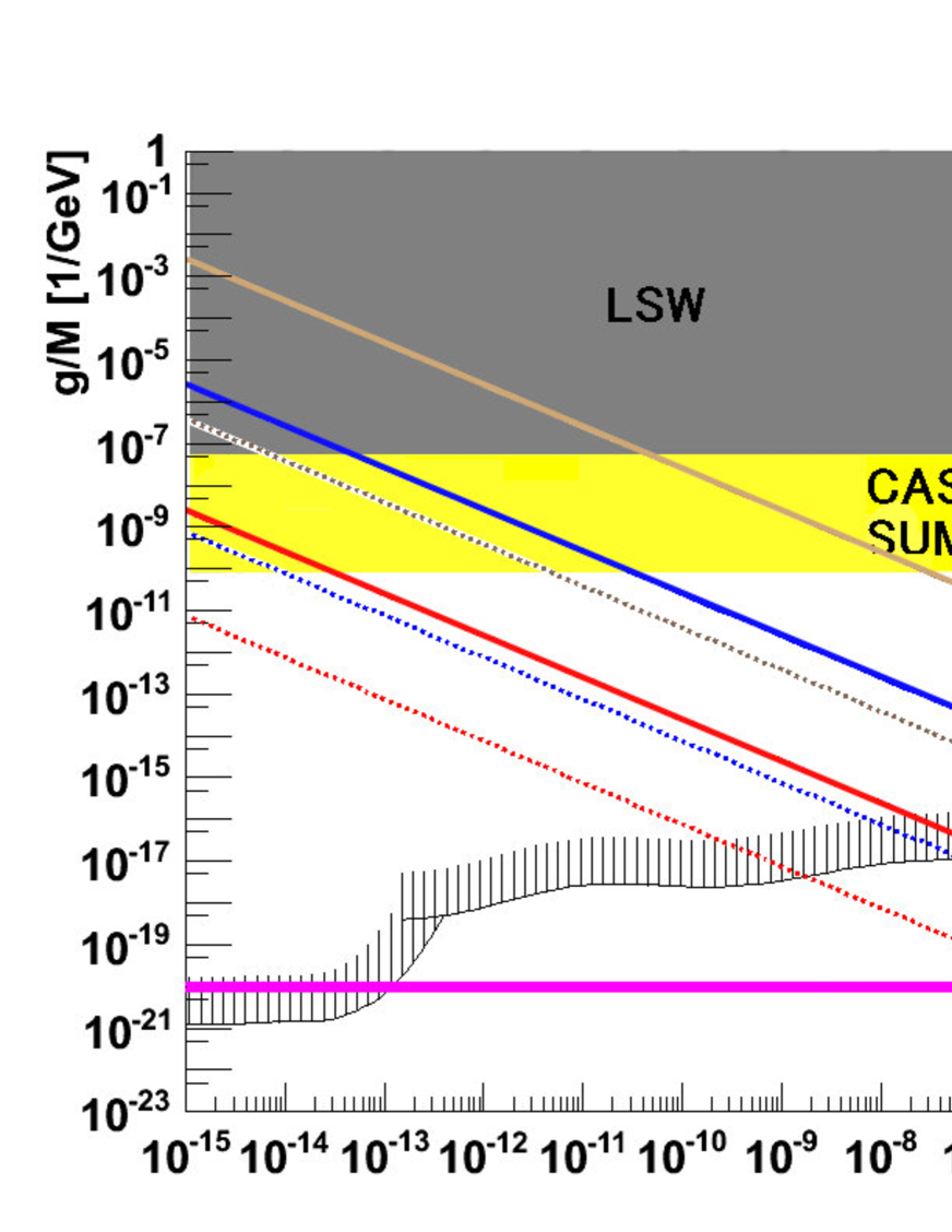
Figure 4: Upper limits of the sensitivities in the $(m,g/M)$ plane by searching for the four-wave mixing process with a single laser shot. The brown, blue and red lines indicate the achievable upper limits with 95% confidence level by assuming no background process is included, when no photon with frequency upshit is observed per single shot focusing, whose laser parameters are summarized in Tab.1 based on the formula Eq.(52) with $C_{mb}=1/2$. Here ${\cal F}_{s}=2\pi$ is used because any ${\cal F}_{S}$ are on the same order as those in the axial symmetric case and the intention of this plot is not in the separation between scalar and pseudoscalar fields. The solid and dashed lines are the cases with short and long focal lengths. The excluded gray, black and yellow domains via the dark field - photon coupling are quoted from AxionReview . The upper limits from the searches for the non-Newtonian force by reinterpreting them based on the effective Yukawa interaction between test bodies FifthYukawa are also shown with the black shaded curves. The limit of the gravitational coupling strength is added by assuming $g\sim{\cal O}(\alpha_{qed})\sim 10^{-2}$ and $M=M_{P}\sim 10^{18}$ GeV as an order estimate based on the model STTL .

Laser parameters	Brown lines	Blue lines	Red lines
production energy	200 J	20 kJ	2 MJ
inducing energy	200 J	20 kJ	2 MJ
inducing spectrum width $\delta u$	0.1	0.1	0.1
pulse duration time $\tau(=\tau_{c}=\tau_{i})$	1 ns	1 ns	1 ns
diameter at the final focusing mirror $d$	40 cm	80 cm	800 cm
intensity at the final focusing mirror	$3.2\times 10^{8}~{}$W/cm2	$8.0\times 10^{9}~{}$W/cm2	$8.0\times 10^{9}~{}$W/cm2
fluence at the final focusing mirror	$0.32~{}$J/cm2	$8.0~{}$J/cm2	$8.0~{}$J/cm2
Short focal length $f$ (mass range)	1.5 m ($<0.22$ eV)	3 m ($<0.22$ eV)	30 m ($<0.22$ eV)
$gm/M$ at 95% C.L. for short focal length	$2.52\times 10^{-27}$	$2.52\times 10^{-30}$	$2.52\times 10^{-33}$
Long focal length $f$ (mass range)	10km ($<32$ $\mu$eV)	10km ($<65$ $\mu$eV)	10km ($<0.65$ meV)
$gm/M$ at 95% C.L. for long focal length	$3.88\times 10^{-31}$	$7.61\times 10^{-34}$	$7.56\times 10^{-36}$

Table 1: Laser parameters to estimate the sensitivity to mass-coupling domains by searching for the four-wave mixing process in the vacuum.

IV Conclusion

We have shown that the sensitivity to dark fields by searching for the four-wave mixing process of laser fields is expected to be able to reach the sub-eV mass range with the coupling strength as weak as that of gravity and even beyond it, if the cutting-edge laser technology is properly combined. Even before reaching extremely high fields, we have many opportunities to test the light cold Dark Matter candidate by the proposed method. This high-sensitivity is essentially realized by the Bosonic nature of laser fields.

As a concluding remark, we emphasize some of features to search for the four-wave mixing process by comparing them with those in high-energy colliders as follows. As an example, let us remind of the Higgs production at LHC as a search for the heavy scalar field.

First, resonance searches in collider experiments are based on measurement of the invariant mass distribution of a produced resonance state. In searching for a resonance state in QPS, in contrast, we have the unavoidable CMS energy uncertainty originating from the uncertainty principle of optical waves compared with the extremely narrow resonance width due to the weakly coupling. We are unable to reconstruct the invariant mass distribution directly, though the interaction probability is still affected by the integrated effect over the possible CMS energy uncertainty. By observing the appearance or disappearance of the four-wave mixing signal, however, one can determine the order of the mass scale from the incident wavelength and the collision geometry, a significant difference from the conventional collider’s approach.

Second, in the case of Higgs at LHC, the dominant production channel is the gluon-gluon fusion process and the produced Higgs resonance state decays into two photons, where both the initial gluons and the final photons are not in degenerate states. Therefore, all fields should be treated incoherently, and the decay process occurs only via spontaneous processes in the vacuum, i.e., two photons in the final state are created from the pure vacuum state $|0\rangle$. On the other hand, in the case of photon-photon interactions under laser fields, all photons are annihilated into and created from the degenerate states. This situation results in the interaction rate with the cubic dependence on the average number of photons included in the laser fields, which is in contrast to the square dependence of the number of charged particles in luminosity of the Fermionic particle colliders. The prime mission of the energy frontier of high energy physics is, of course, to produce new heavy particles, therefore, the realization of the high CMS energy is the most important task, while the sensitivity to weakly coupling fields is sacrificed. The dimensionless intensity included in luminosity is proportional to the square of the number of charged particles per bunch which is typically $\sim 10^{11}$ particles due to the physical limitation by the space-charge effect. Even if we could collide them at most 1GHz over three years data taking period, the integrated dimensionless intensity reaches $(10^{11})^{2}\cdot 10^{9}\cdot 10^{8}=10^{39}$. This indicates that it is practically impossible to reach the sensitivity to cross sections with coupling including $M^{-1}_{P}$. In contrast, by the proposed method, we can expect the dimensionless intensity of $(10^{23})^{3}=10^{69}$ even with a single laser shot including the Avogadro’s number of photons. This manifestly shows how the proposed approach can be sensitive to the weakly coupling interactions.

Therefore, in addition to the present most powerful experimental approach such as heavy boson searches at the high-energy Fermionic collider, the proposed coherent Bosonic collider with the inducing mechanism, simply speaking, four-wave mixing by focused high-intensity laser fields opens up a novel opportunity to bridge particle physics and cosmology in the so far unprobed low-mass and weakly coupling domains under the controllable laboratory environments.

Appendix: Polarization Dependence of Scattering Amplitudes and Axial Asymmetric Factors ${\cal F}_{S}$

Given the scattering configuration illustrated in Fig.3, the Lorentz invariant $s$-channel scattering amplitudes defined in Eq.(2) have the following basic form

$${\cal M}_{S}=-(gM^{-1})^{2}\frac{{\cal V}^{[1]}_{ab}{\cal V}^{[2]}_{cd}}{(p_{1}+p_{2})^{2}+m^{2}},$$ (55)

where $S\equiv abcd$ with $a,b,c,d=1$ or $2$, respectively, denotes a sequence of four-photon polarization states and $m$ is the mass of scalar or pseudoscalar field.

The vertex factors in the numerator for the case of the scalar field exchange ($SC$) are defined as

$${\cal V}^{[1]SC}_{ab}\equiv<p_{2},e_{2}^{(b)}|\frac{1}{4}F_{\mu\nu}F^{\mu\nu}|p_{1},e_{1}^{(a)}>=\frac{1}{2}<p_{2},e_{2}^{(b)}|F_{\mu\nu}|0><0|F^{\mu\nu}|p_{1},e_{1}^{(a)}>$$

$${\cal V}^{[2]SC}_{cd}\equiv<p_{4},e_{4}^{(d)}|\frac{1}{4}F_{\mu\nu}F^{\mu\nu}|p_{3},e_{3}^{(c)}>=\frac{1}{2}<p_{4},e_{4}^{(d)}|F_{\mu\nu}|0><0|F^{\mu\nu}|p_{3},e_{3}^{(c)}>,$$ (56)

while these for the case of the pseudoscalar exchange ($PS$) are given by

$${\cal V}^{[1]PS}_{ab}\equiv<p_{2},e_{2}^{(b)}|\frac{1}{4}F_{\mu\nu}\epsilon^{\mu\nu\rho\sigma}F_{\rho\sigma}|p_{1},e_{1}^{(a)}>=\frac{1}{2}<p_{2},e_{2}^{(b)}|F_{\mu\nu}|0><0|\epsilon^{\mu\nu\rho\sigma}F_{\rho\sigma}|p_{1},e_{1}^{(a)}>$$

$${\cal V}^{[1]PS}_{cd}\equiv<p_{4},e_{4}^{(d)}|\frac{1}{4}F_{\mu\nu}\epsilon^{\mu\nu\rho\sigma}F_{\rho\sigma}|p_{3},e_{3}^{(c)}>=\frac{1}{2}<p_{4},e_{4}^{(d)}|F_{\mu\nu}|0><0|\epsilon^{\mu\nu\rho\sigma}F_{\rho\sigma}|p_{3},e_{3}^{(c)}>.$$ (57)

Let us define the polarization vectors and momentum vectors for four photons in Fig.3 as follows:

$$e_{i}^{(1)}=(0,1,0),$$ (58)

$$e_{1}^{(2)}=(-\cos\vartheta,0,\sin\vartheta),\quad e_{2}^{(2)}=(-\cos\vartheta,0,-\sin\vartheta),$$

$$e_{3}^{(2)}=(-\cos\theta_{3},0,\sin\theta_{3}),\quad e_{4}^{(2)}=(-\cos\theta_{4},0,-\sin\theta_{4}),$$

$$p_{1}=(\omega\sin\vartheta,0,\omega\cos\vartheta;\omega),\quad p_{2}=(-\omega\sin\vartheta,0,\omega\cos\vartheta;\omega),$$

$$p_{3}=(\omega_{3}\sin\theta_{3},0,\omega_{3}\cos\theta_{3};\omega_{3}),\quad p_{4}=(-\omega_{4}\sin\theta_{4},0,\omega_{4}\cos\theta_{4};\omega_{4}).$$ (59)

Based on these vectors, let us summarize basic relations between momenta and polarization vectors with photon labels $i=1,2,3,4$ as follows

$$\left(p_{i}e_{j}^{(1)}\right)=0$$ (60)

for the coplanar condition where the plane determined by $p_{1}$ and $p_{2}$ is the same as that of $p_{3}$ and $p_{4}$,

$$\left(e_{i}^{(1)}e_{j}^{(1)}\right)=1,\mbox{\quad and \quad}\left(e_{i}^{(1)}e_{j}^{(2)}\right)=0,$$ (61)

for any pair $i$, $j$, and

$$\left(e_{i}^{(2)}e_{j}^{(2)}\right)=1\mbox{\quad for\quad}i=j,$$

$$\left(e_{1}^{(2)}e_{2}^{(2)}\right)=\cos 2\vartheta,\left(e_{3}^{(2)}e_{4}^{(2)}\right)=\cos(\theta_{3}+\theta_{4})\equiv\cos\theta_{+},$$

$$\left(e_{1}^{(2)}e_{3}^{(2)}\right)=\cos(\vartheta-\theta_{3}),\left(e_{2}^{(2)}e_{4}^{(2)}\right)=\cos(\vartheta-\theta_{4}),$$

$$\left(e_{1}^{(2)}e_{4}^{(2)}\right)=\cos(\vartheta+\theta_{4}),\left(e_{2}^{(2)}e_{3}^{(2)}\right)=\cos(\vartheta+\theta_{3}).$$ (62)

We then introduce a clock-wise rotation of the $p_{3}$-$p_{4}$ plane from the $p_{1}$-$p_{2}$ plane defined on the $x-z$ plane by the azimuthal angle $\varphi$ varying from 0 to $2\pi$ around the $z$-axis in order to discuss the axial symmetry of the scattering process, when polarization vectors are fixed in an experiment. The rotated vectors are defined as

$$p_{3}(\varphi)=(\omega_{3}\sin\theta_{3}\cos\varphi,-\omega_{3}\sin\theta_{3}\sin\varphi,\omega_{3}\cos\theta_{3};\omega_{3})$$

$$p_{4}(\varphi)=(-\omega_{4}\sin\theta_{4}\cos\varphi,\omega_{4}\sin\theta_{4}\sin\varphi,\omega_{4}\cos\theta_{4};\omega_{4}),$$ (63)

and these result in

$$\left(p_{3}(\varphi)p_{4}(\varphi)\right)=\omega_{3}\omega_{4}(\cos\theta_{+}-1)=\omega^{2}(\cos 2\vartheta-1)$$ (64)

where the last equation is obtained from $(p_{1}+p_{2})^{2}=(p_{3}+p_{4})^{2}$.

With vectors defined above, the vertex factors for the scalar case are expressed as

$${\cal V}_{ab}^{[1]SC} = (p_{1}p_{2})(e_{1}^{(a)}e_{2}^{(b)})-(p_{1}e_{2}^{(a)})(p_{2}e_{1}^{(b)})\qquad\qquad\quad,$$

$${\cal V}_{cd}^{[2]SC} = (p_{3}(\varphi)p_{4}(\varphi))(e_{3}^{(c)}e_{4}^{(d)})-(p_{3}(\varphi)e_{4}^{(c)})(p_{4}(\varphi)e_{3}^{(d)}),$$ (65)

and these for the pseudoscalar case are expressed as

$${\cal V}_{ab}^{[1]PS} = -\epsilon^{\mu\nu\rho\sigma}p_{1\mu}p_{2\rho}e_{1\nu}^{(a)}e_{2\sigma}^{(b)}\qquad\quad$$

$$V_{cd}^{[2]PS} = -\epsilon^{\mu\nu\rho\sigma}p_{3}(\varphi)_{\mu}p_{4}(\varphi)_{\rho}e_{3\nu}^{(c)}e_{4\sigma}^{(d)}.$$ (66)

We are now ready to estimate the factor ${\cal F}_{S}$ included in the partially integrated cross section in Eq.(11). First, we estimate $S=1122$ for the scalar exchange. From the first of Eq.(65), we obtain

$${\cal V}^{[1]SC}_{11}=\omega^{2}(\cos 2\vartheta-1)\equiv{\cal K}\omega^{2}.$$ (67)

With

$$\left(p_{3}(\varphi)e_{4}^{(2)}\right) = -\omega_{3}(\sin\theta_{3}\cos\theta_{4}\cos\varphi+\cos\theta_{3}\cos\theta_{4})$$

$$\left(p_{4}(\varphi)e_{3}^{(2)}\right) = \omega_{4}(\sin\theta_{4}\cos\theta_{3}\cos\varphi+\cos\theta_{4}\cos\theta_{3}),$$ (68)

we get

$$\left(p_{3}(\varphi)e_{4}^{(2)}\right)\left(p_{4}(\varphi)e_{3}^{(2)}\right)=-\omega_{3}\omega_{4}\{(1+\cos^{2}\varphi)\sin\theta_{3}\sin\theta_{4}\cos\theta_{3}\cos\theta_{4}$$

$$+(\sin^{2}\theta_{3}\cos^{2}\theta_{4}+\sin^{2}\theta_{4}\cos^{2}\theta_{3})\cos\varphi\},$$ (69)

and then the second vertex factor in the second of Eq.(65) is expressed as

$${\cal V}^{[2]SC}_{22}=\omega_{3}\omega_{4}\{\cos\theta_{+}(\cos\theta_{+}-1)+(1+\cos^{2}\varphi)\sin\theta_{3}\sin\theta_{4}\cos\theta_{3}\cos\theta_{4}$$

$$+(\sin^{2}\theta_{3}\cos^{2}\theta_{4}+\sin^{2}\theta_{4}\cos^{2}\theta_{3})\cos\varphi\}.$$ (70)

For $\varphi=0$, this coincides with $|{\cal V}^{[1]SC}_{11}|$ via the relation

$${\cal V}^{[2]SC}_{22}(\varphi=0) = \omega_{3}\omega_{4}\{\cos\theta_{+}(\cos\theta_{+}-1)+\sin^{2}\theta_{+}\}$$ (71)

$$= \omega_{3}\omega_{4}(1-\cos\theta_{+})=\omega^{2}(1-\cos 2\vartheta)=-{\cal K}\omega^{2}.$$

For a small $\vartheta$ we take the following approximation: $\sin\theta_{3}\sim\sqrt{{\cal R}}\vartheta$ and $\sin\theta_{4}\sim 1/\sqrt{{\cal R}}\vartheta$ from Eq.(39) and (41), and this results in $\cos\theta_{+}$ as

$$\cos\theta_{+}\sim 1-\vartheta^{2}(1+\hat{{\cal R}}),$$ (72)

with

$$\hat{{\cal R}}\equiv\frac{1}{2}({\cal R}+{\cal R}^{-1}).$$ (73)

We then approximate Eq.(Appendix: Polarization Dependence of Scattering Amplitudes and Axial Asymmetric Factors ${\cal F}_{S}$) as

$${\cal V}^{[2]SC}_{22}\sim\omega_{3}\omega_{4}\vartheta^{2}\{\cos^{2}\varphi+(2\cos\varphi-1)\hat{{\cal R}}\}\equiv\omega_{3}\omega_{4}\vartheta^{2}F(\varphi).$$ (74)

This is consistent with the approximation of Eq.(71) for a small $\vartheta$

$${\cal V}^{[2]SC}_{22}(\varphi=0)\sim\omega_{3}\omega_{4}\vartheta^{2}(1+\hat{{\cal R}}).$$ (75)

By taking the square of the factorized second vertex factor, we then naturally define the factor ${\cal F}_{S}$ for the scalar case

$${\cal F}^{SC}_{1122}\equiv\int^{2\pi}_{0}F^{2}(\varphi)d\varphi\sim 2\pi\left(\frac{3}{8}+3\hat{{\cal R}}^{2}-\hat{{\cal R}}\right).$$ (76)

Second, let us estimate S=1212 for the pseudoscalar field exchange as follows. From the first of Eq.(66) with the vector definitions above, we obtain the first vertex factor as

$${\cal V}_{12}^{[1]PS} = -p_{1\mu}p_{2\rho}\epsilon^{\mu y\rho\sigma}e_{2\sigma}^{(2)}=-p_{1\mu}p_{2\rho}\left[\rule[-1.00006pt]{0.0pt}{11.99998pt}\epsilon^{\mu y\rho x}(-\cos\vartheta)+\epsilon^{\mu y\rho z}(-\sin\vartheta)\right]$$ (77)

$$= p_{2\rho}\left[\rule[-1.00006pt]{0.0pt}{11.99998pt}\left(p_{10}\epsilon^{0y\rho x}+p_{1z}\epsilon^{zy\rho x}\right)\cos\vartheta+\left(p_{10}\epsilon^{0y\rho z}+p_{1x}\epsilon^{xy\rho z}\right)\sin\vartheta\right]$$

$$= p_{2\rho}\left[\rule[-1.00006pt]{0.0pt}{11.99998pt}\left(-\omega\epsilon^{0y\rho x}+\omega\cos\vartheta\epsilon^{zy\rho x}\right)\cos\vartheta+\left(-\omega\epsilon^{0y\rho z}+\omega\sin\vartheta\epsilon^{xy\rho z}\right)\sin\vartheta\right]$$

$$= \left[\rule[-1.00006pt]{0.0pt}{11.99998pt}\left(-\omega\epsilon^{0yzx}p_{2z}+\omega\cos\vartheta\epsilon^{zy0x}p_{20}\right)\cos\vartheta+\left(-\omega\epsilon^{0yxz}p_{2x}+\omega\sin\vartheta\epsilon^{xy0z}p_{2z}\right)\sin\vartheta\right]$$

$$= \omega^{2}\left[\rule[-1.00006pt]{0.0pt}{11.99998pt}\left(-\cos\vartheta+\cos\vartheta\right)\cos\vartheta+\left(-\sin\vartheta-\sin\vartheta\right)\sin\vartheta\right]=-2\omega^{2}\sin^{2}\vartheta.$$

We also get the second vertex factor from the second of Eq.(66) with the vector definitions above as follows

$${\cal V}_{12}^{[2]PS} = -\epsilon^{\mu\nu\rho\sigma}p_{3\mu}p_{4\rho}e_{3\nu}^{(1)}e_{4\sigma}^{(2)}=-\epsilon^{\mu y\rho\sigma}p_{3\mu}p_{4\rho}e_{4\sigma}^{(2)}$$ (78)

$$= -\left(-\epsilon^{\mu y\rho x}\cos\theta_{4}-\epsilon^{\mu y\rho z}\sin\theta_{4}\right)p_{3\mu}p_{4\rho}$$

$$= \left[\rule[-1.00006pt]{0.0pt}{11.00008pt}\left(\epsilon^{0y\rho x}\cos\theta_{4}+\epsilon^{0y\rho z}\sin\theta_{4}\right)p_{30}+\left(\epsilon^{zy\rho x}\cos\theta_{4}p_{3z}+\epsilon^{xy\rho z}\sin\theta_{4}p_{3x}\right)\right]p_{4\rho}$$

$$= -\omega_{3}\left(\epsilon^{yzx}p_{4z}\cos\theta_{4}+\epsilon^{yxz}p_{4x}\sin\theta_{4}\right)+4\left(\epsilon^{zy0x}\cos\theta_{4}p_{3z}+\epsilon^{xy0z}p_{3x}\right)p_{40}$$

$$= -\omega_{3}\omega_{4}\left[\rule[-1.00006pt]{0.0pt}{11.00008pt}\left(\cos^{2}\theta_{4}+\sin^{2}\theta_{4}\cos\varphi\right)+\left(-\cos\theta_{4}\cos\theta_{3}+\sin\theta_{4}\sin\theta_{3}\cos\varphi\right)\right]$$

$$= -\omega_{3}\omega_{4}\left[\rule[-1.00006pt]{0.0pt}{11.00008pt}\cos\theta_{4}(-\cos\theta_{3}+\cos\theta_{4})+\sin\theta_{4}(\sin\theta_{4}+\sin\theta_{3})\cos\varphi\right].$$

For $\varphi=0$, we find

$${\cal V}_{12}^{{[2]PS}}(\varphi=0) = -\omega_{3}\omega_{4}\left(-\cos\theta_{3}\cos\theta_{4}+\cos^{2}\theta_{4}+\sin^{2}\theta_{4}+\sin\theta_{3}\sin\theta_{4}\right)$$ (79)

$$= -\omega_{3}\omega_{4}\left(1-\cos\theta_{+}\right)=-\omega^{2}\left(1-\cos 2\vartheta\right)={\cal K}\omega^{2}.$$

If we use the same approximations as the scalar case, the second vertex factor is approximated as

$${\cal V}_{12}^{{[2]PS}}\sim-\omega_{3}^{2}\omega_{4}^{2}\vartheta^{2}\{\check{{\cal R}}+({\cal R}^{-1}+1)\cos\varphi\}\equiv-\omega_{3}^{2}\omega_{4}^{2}\vartheta^{2}G(\varphi),$$ (80)

with

$$\check{{\cal R}}\equiv\frac{1}{2}({\cal R}-{\cal R}^{-1}).$$ (81)

This is consistent with the approximation of Eq.(79) for a small $\vartheta$

$${\cal V}_{12}^{{[2]PS}}(\varphi=0)\sim-\omega_{3}\omega_{4}\vartheta^{2}(1+\hat{{\cal R}}).$$ (82)

Again by taking the square of the second vertex factor, we then naturally define the factor ${\cal F}_{S}$ for the pseudoscalar case

$${\cal F}^{PS}_{1212}\equiv\int^{2\pi}_{0}G^{2}(\varphi)d\varphi\sim 2\pi\{\check{{\cal R}}^{2}+\frac{1}{2}({\cal R}^{-1}+1)^{2}\}.$$ (83)

Let us confirm relations for the case of $\varphi=0$ as follows: The ratio of the invariant amplitude of the pseudoscalar case to the scalar case as

$$\frac{{\cal M}^{PS}_{1212}(\varphi=0)}{{\cal M}^{SC}_{1122}(\varphi=0)}=\frac{{\cal V}^{[1]PS}_{12}{\cal V}^{[2]PS}_{12}}{{\cal V}^{[1]SC}_{11}{\cal V}^{[2]SC}_{22}}=\frac{-2\sin^{2}\vartheta\omega^{2}\cdot{\cal K}\omega^{2}}{{\cal K}\omega^{2}\cdot-{\cal K}\omega^{2}}\sim 1$$ (84)

for a low-mass case with a small $\vartheta$. The other non-vanishing invariant amplitudes are limited to $S=1111,2222,1122,2211$ for the scalar exchange and $S=1212,1221,2121,2112$ for the pseudoscalar case. These relations can be confirmed by repeating routine calculations performed above.

References

- (1) http://lambda.gsfc.nasa.gov/product/map/current/best_params.cfm.
- (2) L. Amendola and S. Tsujikawa, Dark Energy, Cambirdge University Press (2010).
- (3) R. R. Caldwell, R. Dave, and P. J. Steinhardt, Phys. Rev. Lett. 90, 1582 (1998); L. Wang, R. R. Caldwell, J. P. Ostriker, and P. J. Steinhardt, Astrophys. J. 530, 17 (2000).
- (4) Y. Fujii and K. Maeda, The Scalar-Tensor Theory of Gravitation Cambridge Univ. Press (2003).
- (5) Y. Fujii, Phys. Lett. B 660, 87 (2008), arXiv 0709.2211.
- (6) C. Brans and R. H. Dicke, Phys. Rev. 124, 925 (1961).
- (7) A short summary of STTL is available. For example, see Y. Fujii, arXiv:0908.4324 [astro-ph.CO].
- (8) Y. Nomura, T. Watari and T. Yanagida, Phys. Lett. B 484, 103 (2000); K. Choi, Phys. Rev. D 62, 043509 (2000); J. E. Kim and H. P. Nilles, Phys. Lett. B 553, 1 (2003); L. J. Hall, Y. Nomura and S. J. Oliver, Phys. Rev. Lett. 95, 141302 (2005).
- (9) P. Brax, C. van de Bruck, A. C. Davis, J. Khoury and A. Weltman, Phys. Rev. D 70, 123518 (2004).
- (10) H. J. de Vega, N. G. Sanchez, arXiv:astro-ph/0701212.
- (11) Y. Fujii, Nature Phys. Sci. 234, 5 (1971).
- (12) E. Fischbach and C. Talmadge. The search for non-Newtonian gravity, AIP Press, Springer-Verlag, New York (1998).
- (13) Y. Fujii and K. Homma, Prog. Theor. Phys. 126: 531-553 (2011), arXiv:1006.1762 [gr-qc].
- (14) R. D. Peccei and H. R. Quinn, Phys. Rev. Lett. 38, 1440 (1977).
- (15) For example, see Figure 2 and section 4 in J. Jaeckel and A. Ringwald, The Low-Energy Frontier of Particle Physics, Ann. Rev. Nucl. Part. Sci. 60, 405 (2010) arXiv:1002.0329 [hep-ph].
- (16) Mark P. Hertzberg, Max Tegmark, and Frank Wilczek, Phys. Rev. D 78, 083507 (2008); Olivier Wantz and E. P. S. Shellard, Phys. Rev. D 82, 123508 (2010).
- (17) K. Homma, D. Habs, T. Tajima, Appl. Phys. B 106:229-240 (2012), (DOI: 10.1007/s00340-011-4567-3),arXiv:1103.1748 [hep-ph].
- (18) Amnon Yariv, Optical Electronics in Modern Communications (Oxford University Press, 1997).
- (19) R. J. Glauber, Phys. Rev. 131 (1963), 2766.
- (20) Sylvie A. J. Druet and Jean-Pierre E. Taran, Prog. Quant. Electr. Vol.7, pp. 1-72 (1981).
- (21) F. Moulina and D. Bernardb, Opt. Commun. 164, 137-144 (1999).
- (22) E. Lundström et al., Phys. Rev. Lett. 96, 083602 (2006); J. Lundin et al., Phys. Rev. A74, 043821 (2006).
- (23) D. Bernard et al., Eur. Phys. J. D10, 141 (2000).
- (24) K. Homma, D. Habs, G. Mourou, H. Ruhl, and T. Tajima, Prog. Theor. Phys. Suppl. No. 193, (2012); http://www.extreme-light-infrastructure.eu/; http://www.int-zest.com/index.html.
- (25) P. Gibbson, Short Pulse Laser Interactions with Matter AN INTRODUCTION (Imperial College Press, 2005).
- (26) Dupays A, Masso E, Redondo J, Rizzo C. Phys. Rev. Lett. 98, 131802 (2007).
- (27) G. Ruoso et al., Z. Phys. C56, 505 (1992); R. Cameron et al., Phys. Rev. D47, 3707 (1993); M. Fouche et al. (BMV Collab.), Phys. Rev. D78, 032013 (2008); P. Pugnat et al. (OSQAR Collab.), Phys. Rev. D78, 092003 (2008); A. Chou et al. (GammeV T-969 Collab), Phys. Rev. Lett. 100, 080402 (2008); A. Afanasev et al. (LIPSS Collab.), Phys. Rev. Lett. 101, 120401 (2008); K. Ehret et al. (ALPS Collab.), Phys. Lett. B689, 149 (2010).
- (28) S. Moriyama et al., Phys. Lett. B434, 147 (1998); Y. Inoue et al., Phys. Lett. B536, 18 (2002); M. Minowa et al., Phys. Lett. B668, 93 (2008).
- (29) S. Andriamonje et al. (CAST Collab.), JCAP 0704, 010 (2007); E. Arik et al. (CAST Collab.), JCAP 0902, 008 (2009); E. Arik et al. (CAST Collab.), Phys. Rev. Lett. 107, 261302 (2011).
- (30) S. Asztalos et al., Phys. Rev. D69, 011101 (2004); S.J. Asztalos et al., Phys. Rev. Lett. 104, 041301 (2010);
- (31) Table 33.3 in K. Nakamura et al. (Particle Data Group), J. Phys. G 37, 075021 (2010) and 2011 partial update for the 2012 edition.
- (32) http://www.clf.rl.ac.uk/New+Initiatives/The+Vulcan+10+Petawatt+Project/18344.aspx
- (33) http://www.eli-np.ro/documents/ELI-NP-WhiteBook.pdf
- (34) http://www.extreme-light-infrastructure.eu/pictures/Grand-Challenges-Meeting-Report-id66.pdf
- (35) http://www.ile.osaka-u.ac.jp/zone1/activities/facilities/spec_e.html
- (36) http://www.clf.stfc.ac.uk/Facilities/Vulcan/Vulcan+laser/12250.aspx
- (37) http://www.lle.rochester.edu/omega_facility/omega/
- (38) http://int-zest.com/pdf/le-garrec.pdf
- (39) http://www-lmj.cea.fr/index-en.htm
- (40) https://lasers.llnl.gov
- (41) Mourou, G., Fisch, N., Malkin, V.M. Toroker, Z., Khazanov, E. A., Sergeev, A. M., Tajima, T., and Le Garrec, B., Opt. Comm. 285, 720 (2012).
- (42) https://www.izest.polytechnique.edu/izest-home/ican/ican-94447.kjsp?RF=1332339530225
- (43) T. Tajima and J. Dawson, Phy. Rev. Lett. 43, 267 (1979).
- (44) T. Tajima and K. Homma, Int. J. Mod. Phys. A vol. 27, No. 25, 1230027 (2012).
- (45) http:www.izest.polytechnique.edu