An Arecibo Survey for Zeeman Splitting in OH Megamaser Galaxies

Abstract

We present the results of a comprehensive survey using the Arecibo Observatory for Zeeman splitting of OH lines in OH megamasers (OHMs). A total of seventy-seven sources were observed with the Arecibo telescope. Of these, maser emission could not be detected for eight sources, and two sources were only ambiguously detected. Another twenty-seven sources were detected at low signal-to-noise ratios or with interference that prevented placing any useful limits on the presence of magnetic fields. In twenty-six sources, it was possible to place upper limits on the magnitude of magnetic fields, typically between 10–30 mG. For fourteen sources, the Stokes $V$ spectra exhibit features consistent with Zeeman splitting. Eleven of these fourteen are new detections, and the remaining three are re-detections of Stokes $V$ detections in Robishaw et al. (2008). Among confident new detections, we derive magnetic fields associated with maser regions with magnitudes ranging from 6.1–27.6 mG. The distribution of magnetic field strengths suggests the magnetic fields in OH masing clouds in OHMs are larger than those in Galactic OH masers. The results are consistent with magnetic fields playing a dynamically important role in OH masing clouds in OHMs.

1. Introduction

This work follows that of Robishaw et al. (2008) (hereafter R08), who detected Zeeman splitting in a sample of five OH megamasers, and is structured similarly for ease of reference to that work. OH megamasers (OHMs) are powerful extragalactic masers that operate in the 18-cm transitions of the hydroxyl molecule, with typical luminosities of order $\log(L_{\rm OH}/L_{\odot})=3$—one hundred million ($10^{8}$) times greater than the luminosity of OH masers in the Milky Way. OHMs are found in luminous and ultra-luminous infrared galaxies (LIRGs and ULIRGs), classes of galaxies with $\log(L_{\rm FIR}/L_{\odot})>$ 11 and $\log(L_{\rm FIR}/L_{\odot})>12$, respectively. Among these galaxies, OHMs have a preference for the most far infrared luminous (Darling & Giovanelli, 2002a).

OHM emission occurs primarily in the 1667 MHz main line transition, with the 1665 MHz main line either weaker or absent (Darling & Giovanelli, 2002b), and the satellite lines at 1612 MHz and/or 1720 MHz only detected in a few nearby OHMs Baan et al. (1987, 1992); Martin et al. (1989). VLBI observations of Arp 220, IRAS F17208–0014, and III Zw 35, all with redshifts $z<0.05$, find a combination of compact 1667 MHz emission on parsec sized scales and diffuse 1665 MHz and 1667 MHz emission on scales of hundreds of parsecs, and also see evidence for Keplerian motion in rotating maser rings (Lonsdale et al., 1998; Diamond et al., 1999; Pihlström et al., 2001; Momjian et al., 2006). Markarian 231, meanwhile, contained no compact emission in VLBI observations by Lonsdale & Smith (2003) that had a physical resolution of roughly 80 pc, meaning emission is coming from regions larger than 80 pc. Pihlström et al. (2005) performed VLBI observations of IRAS F12032+1707 and IRAS F14070+0525, which are the third most distant and most distant OHMs, respectively, with $z>0.20$. They found that the majority of emission from IRAS F12032+1707 is ordered and compact on scales of less than 100 pc, while most of the emission in IRAS F14070+0525 is resolved out. Parra et al. (2005) modeled the emission of III Zw 35 as arising from a rotating starburst ring with clumpy OH clouds, which Lo (2005) suggests could explain other sources as well. In the context of the clumpy model of OHMs, Lockett & Elitzur (2008) explained the observed line ratios of OHMs as being produced through 53 $\mu$m radiative pumping produced by dust with a minimum temperature of 45 K, and overlap of lines with $\sim 20\;{\rm km\;s}^{-1}$ linewidths.

[U]LIRGs that host OHMs are predominantly merging systems, in which molecular gas is funneled to a central merging nucleus. One or both of star formation and active galactic nucleus (AGN) activity produce far infrared and radio continuum emission (Darling & Giovanelli, 2002a, 2006)—evidence for AGN or star formation activity dominating in OHMs has been conflicting. Baan et al. (1998) used optical spectroscopy to look at the source of nuclear activity in OHMs, and found a preference for AGN among their sample of 42 galaxies. Darling & Giovanelli (2006) also studied optical spectra of OHMs, this time comparing to a sample of non-masing [U]LIRGs, and found no significant difference between the OHM hosts and non-masing galaxies. Vignali et al. (2005) observed seven OHMs with Chandra, detecting only one source weakly, a finding that is consistent with galaxies powered by star formation or low-luminosity AGN. Kandalian et al. (2007) looked at a larger sample of x-ray observations of 22 OHMs, using both Chandra and XMM-Newton data, and observed a weak relationship between the x-ray luminosity and OH luminosity that favored an AGN contribution in some sources, but noted that galaxies may host OHMs as a result of either AGN activity or rapid star formation. Willett et al. (2011a, b) compared OHM hosts and non-masing ULIRGs in the mid-infrared, finding that the fraction of AGN in OHMs is lower than that of non-masing ULIRGs, and also demonstrated support for a minimum dust temperature comparable to that used in the modeling in Lockett & Elitzur (2008). Altogether, the most recent work points to star formation powering OHMs, though AGN activity may still play an important role. In trying to distinguish OHM hosts from non-masing galaxies of similar luminosity, Darling (2007) examined the conditions of the molecular gas, finding a clearer distinction between the two populations based on high mean molecular gas densities. Typical OHM hosts have $\bar{n}\left({\rm H_{2}}\right)=10^{3}$–$10^{4}\;\;{\rm cm}^{-3}$ and high dense gas fractions, with half of galaxies that have $L_{\rm HCN}/L_{\rm CO}>0.07$ also hosting OHMs.

R08 noted that the conditions in which OHMs reside, particularly the high energy and molecular gas densities, suggest the presence of strong magnetic fields. Minimum energy arguments made using VLA observations of synchrotron emission argue for minimum volume averaged magnetic field strengths of 1 mG in the central 100 pc of ULIRGs (Condon et al., 1991). Thompson et al. (2006) argued that producing the FIR-radio correlation for starburst galaxies requires significant fine-tuning if magnetic fields are not significantly larger than the minimum energy estimates. They further show that for magnetic fields to be dynamically important relative to gravity, as in the Milky Way, the magnetic fields in Arp 220 or a similar galaxy would be of order 30 mG. These arguments for fields in [U]LIRGs with magnitudes between 1–30 mG provided a compelling case to search for Zeeman splitting in [U]LIRGs, and in particular, observe OHM lines. The hydroxyl molecule has a relatively large magnetic dipole moment, and OHMs provide bright, narrow lines in which Zeeman splitting may be detected.

In an effort to directly Zeeman splitting and measure line-of-sight magnetic fields in [U]LIRGs, R08 used the Arecibo telescope and the Green Bank Telescope to perform Full-Stokes observations for eight OHMs. They detected magnetic fields with a median strength of $\simeq$ 3 mG in five of the eight observed galaxies, and the strongest detected field had a magnitude of 17.9 mG. Their results confirmed that Full-Stokes observations of OHMs provide a viable way to directly measure magnetic fields in [U]LIRGs, even if magnetic fields are not of equal dynamical importance to gravity in the ISM of [U]LIRGs. Here, we go further, observing seventy-seven known extragalactic OH masers, including re-observations of six of the sources from R08. Eight OHMs are not detected at all, primarily as a result of increased radio-frequency interference (RFI) since their discovery. Three sources exhibit features in their Stokes $V$ spectra consistent with Zeeman splitting, but in which we are only marginally confident. Eleven OHMs have Stokes $V$ features that we confidently associate with Zeeman splitting, including re-detections of Zeeman splitting in three OHMs observed in R08. One source, IRAS F10173+0829, showed apparent Zeeman splitting in the observations of R08, but re-observation showed that the apparent features were interference. The remaining sources were detected in Stokes $I$, but did not show significant Zeeman splitting detections.

2. Sources

The seventy-seven OHMs make up the entire sample known at the time of observations that are observable with the Arecibo telescope in Puerto Rico. All but two of the targets were taken from the OHM survey and compilation of past detections presented in Darling & Giovanelli (2000, 2001, 2002a) (hereafter DG00, DG01, DG02). The two exceptions are the only two Arecibo accessible sources that have been discovered in the decade since (Willett, 2012). While the choice to use only Arecibo excludes some viable targets, the results of R08 showed that detecting magnetic fields using Zeeman splitting of OHMs requires a level of sensitivity more easily achieved with Arecibo.

3. Observations

We used the $L$-band wide receiver on the 305-meter Arecibo telescope in full-Stokes mode to observe all known OH megamasers at declinations accessible to Arecibo, over a period spanning December 2007–December 2009. The interim correlator was set up to observe four different bands: one 12.5 MHz band, centered halfway between the 1665 and 1667 MHz, and three 6.25 MHz bands, centered at 1612, 1667, and 1720 MHz. This set-up allowed simultaneous observation of all four ground state OH maser lines and all four Stokes parameters, $I$, $Q$, $U$, and $V$. This differs from the correlator setup used by R08, which focused only on the main lines, and had a range of bandwidths that depended upon the velocity extent of the source. The uniformity of the setup used here eased reduction and analysis. This work focuses on the 1665 MHz and 1667 MHz lines, as there were no Zeeman detections in the satellite lines at 1612 MHz or 1720 MHz. A future work will present the results of the observations of the satellite lines.

We spent equal time on and off source, switching position every 4 minutes. The off source position had the same declination and a right ascension 4 minutes east of the source, which kept the hour angles of on and off source observations nearly equal. The integration time was 1 second, chosen to allow for elimination of RFI that appeared on short time scales.

4. Data Reduction

Many of the details of the data reduction are well described in R08. This includes calibration of spectra, RFI removal, bandpass and gain correction, and fitting Gaussian components to the Stokes $I$ profiles. The discussion here will focus on describing new components of the data reduction, and mostly does not repeat the description in R08 in cases where the procedure used in reducing the data in this paper was identical to that in R08. Section 4.1 of R08, describing calibration, and 4.3, describing bandpass and gain correction, are omitted entirely.

We use the classical definition of Stokes $I$, which is the sum, rather than the average, of two orthogonal polarizations. Our flux densities are thus twice those of most previously published work, but are consistent with the choice of R08. We take the IAU definition of Stokes $V$, with $V=RHCP-LHCP$. Following the IEEE definitions $RHCP$ is clockwise rotation and $LHCP$ is counterclockwise rotation of the electric field vector along the direction of propagation.

4.1. RFI removal

The data were examined for RFI in various stages. First, the on/off pairs of 1 second records were flagged for RFI and checked for significant rippling caused by the Sun or Moon being within the beam sidelobes. At this point, the data reduction forked: within each on/off pair of 4 minute records, the 1  second records were averaged together to form a single 4 minute spectrum, and also combined by taking the median to form a second 4 minute spectrum for the same data. In cases where the RFI is limited, the average spectrum tended to be less noisy, but forming a composite spectrum from the median of the 1 second integrations was clearly better for sources with significant narrow-band RFI.

Each source was typically observed for a few hours. This resulted in $\sim$10–20 4 minute on and off spectra for each source. These too were combined in the same manner as the 1 second spectra, either by taking the average or the median. Applying these choices to each set of mean or median 4 minute spectra resulted in four different final spectra for each source at a given frequency and polarization: mean/mean, mean/median, median/mean, median/median. Of these four options, the spectrum with the least noise was selected.

4.2. Confidence tests

Many of the Zeeman measurements presented here represent marginal detections. We describe here some of the primary obstacles to determining magnetic field strengths, and tests applied to the data and fits that validate the results.

4.2.1 Broadband rippling

Many of the Stokes $V$ spectra contain ripples of characteristic size $\sim 0.3$–1 MHz that can masquerade as Zeeman splitting of broad OHM components, and represent the most serious source of systematic error in estimating magnetic fields. The best fit fields to these ripples in the Stokes $V$ spectra are often in excess of 50 milligauss. These ripples are easily spotted by eye in most situations, but can confuse magnetic field fits in sources with particularly rich spectra. For this reason, magnetic field fits associated with spectral features wider than $0.3$ MHz are all considered to be untrustworthy. This choice is also physically motivated, in that particularly wide maser lines are likely produced by blending from many masing clouds, and are less likely to provide a detectable line-of-sight Zeeman splitting signal.

4.2.2 Spectral shifting

Even after removing the broadest ripples, there are Stokes $V$ spectra with structured noise on smaller frequency scales that can confuse interpretation. In some cases, noisy structure in Stokes $V$ may be coincidentally lined up with features in the Stokes $I$ spectrum, and produce claimed magnetic field detections. To identify instances of dubious magnetic field claims, we ran our fitting procedure for Zeeman splitting with the Stokes $V$ spectrum shifted relative to the Stokes $I$ spectrum for all sources. With 2048 channels, this produces 2048 different fits to features in Stokes $V$. For each set of fits, we selected the features narrower than $0.3$ MHz, found the associated signal to noise ratio for the magnetic fields of each narrow component, and produced an overall quality of fit at each shift. For sources where non-zero shifts produced fits of comparable quality to the fits with no shift, the reported fields were regarded as highly dubious. In Section 5.1.7, all sources for which we claim a magnetic field detection were best fit when no shift was applied between the Stokes $I$ and $V$ spectra. Other sources with claimed magnetic fields, but which were also well fit when the Stokes $I$ and $V$ were shifted relative to one another, were considered Stokes $V$ non-detections or marginal detections, depending on other factors. An example of this process is shown in Figure 1. The source in the top panel is not fit particularly well at any one shift, whereas the source in the bottom panel is only well fit when no shift is applied, providing confidence that the features being fit are real. The full fits for these sources are shown in Sections 5.1.5 and 5.1.7.

Figure 1.— The average signal-to-noise ratios of fitted fields to narrow components in the Stokes $I$ and $V$ spectra of IRAS F23028+0725 (top panel) and IRAS F09039+0503 (bottom panel) are plotted for fits when the Stokes $I$ and $V$ spectra are shifted relative to each other. The overall fit quality at no shift for F23028+0725 is mediocre, and the fits are marginally better when the spectra are shifted relative to each other, suggesting that the features being fit in the Stokes $V$ spectrum are not Zeeman splitting. The fits for F09039+0503 are at their best for no shift, and no other shift produces fits of comparable quality.

4.2.3 Comparison of overlapping spectra

For each source observed, there was a total of 25 MHz of spectral coverage, with two 6.25 MHz bands covering the OH satellite lines at rest frequencies of 1612 and 1720 MHz, and the broad 12.5 MHz band that encompassed both main lines at 1665 and 1667 MHz. With sources spread out over a redshift range of 0.007–0.265, the highest observed frequency was 1711 MHz, and the minimum was 1271 MHz. Just over 90% of this range was covered by at least one source, including the entire range between 1351.8 MHz–1663.7 MHz. Moreover, 73% of this band was covered by at least two sources, and 50% was covered by at least four sources.

This overlapping coverage was a valuable tool in RFI identification. Spectra with features of unclear origin could be compared to spectra of other sources in the same frequency range. If a similar feature appeared in both spectra, then it strongly suggests interference. Comparing overlapping spectra of different sources was critical in discovering that the Stokes $V$ features of IRAS F10173+0829, reported in R08, were actually interference. A rough characterization of RFI severity across the frequency range in the survey can be seen in Figure 2.

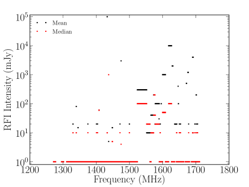
Figure 2.— The spectral coverage of the survey is shown here, along with the RFI environment at Arecibo during observations. Areas with observations and no observed RFI are plotted at a default level of 1 mJy, as that was the typical rms error for RFI free data. At frequencies where RFI was present in at least one data set, the approximate amplitude of the most severe RFI is shown. For a couple of wide regions with severe RFI, such as that between 1524–1552 MHz, the value plotted is typical of the large RFI spikes throughout the frequency range, but RFI of that amplitude was not necessarily observed in each channel.

4.2.4 Field sign

In a survey of Zeeman splitting in Galactic OH masers, Fish & Reid (2006) tested for unknown systematics in their data by counting how many Zeeman pairs had greater flux in the LCP component, how many had greater flux in the RCP component, and comparing their result to the expectation that the each possibility was equally likely. We performed a similar test, counting the number of positive and negative magnetic fields derived, and comparing the results with the binomial distribution.

For $N$ fields and an equal likelihood of positive or negative fields, the probability of a positive field is $p=0.5$, the expected number of positive fields is $Np$, the expected number of negative fields is $N(1-p)$, and their variance is $Np(1-p)$. For all sources, we fit a total of 373 Gaussian components, and a magnetic field estimate was made for each component, giving an expected number of $186.5\pm 9.7$ for positive and negative fields. Of derived fields, 172 had positive sign, and 201 were negative in sign, which are not statistically significant deviations. Likewise, for magnetic field components we considered a detection, there were a total of 35 derived fields. Compared to an expectation of $17.5\pm 2.1$, 19 were positive in sign and 16 were negative, very close to the expected distribution.

4.2.5 Bootstrap resampling

An often used technique to distinguish a source of broadband interference from one of astrophysical interest is to split a dataset in half, and check that the feature is roughly the same strength throughout the observation. When looking for very low SNR features, this method proved to be only marginally helpful, as the fluctuations in amplitude for a low SNR astrophysical signal due to noise might be similar to those expected from broadband interference. As an extension of this, we bootstrap resampled our spectra, rather than splitting the data in to two halves.

Bootstrapping is a resampling method that can be used for estimating confidence intervals associated with a statistic (Efron & Tibshirani, 1993). For a statistic such as the median, bootstrap resampling makes it possible to characterize uncertainty, despite there being no formal way to do so. The procedure is relatively straightforward. Given a sample of $n$ observations, x = ($x_{1},x_{2},...,x_{n}$), the empirical probability of observing each of the $n$ values is $1/n$. A bootstrap sample of x is made up of $n$ values drawn randomly from x. One of the original observations may be drawn more than once, or not at all, in this bootstrap sample. To build a distribution of values for some statistic, such as the median, take the median of the original sample as well as the median of each of many bootstrap samples. This sampled distribution of the median measurements provides an estimate of the uncertainty in the measurement of the median.

As the spectrum for each OHM was made by combining 4 minute spectra, either using the mean or median, we treated each of the 4 minute spectra as an individual observation. As discussed above, for some sources, taking the median of those 4 minute spectra produced a spectrum with less noise, usually because it better handles RFI, while for some sources the mean spectra were less noisy; the “measurement” in this case is whichever of the two was better. We then took 1000 bootstrap samples of that measurement. The resultant lower and upper limits are in a few cases useful in establishing whether a broad spectral feature is OH emission. We performed similar resampling in checking the derived errors of magnetic field estimates. For sources with claimed magnetic field detections, the Stokes $I$ and Stokes $V$ spectra were jointly resampled, and the magnetic field derivation procedure described below was applied. The error from bootstrap resampling was consistently comparable to those reported in the fitting procedure.

4.3. Fitting Gaussian Components to Stokes $I$ Profiles

We followed the same general guidelines given in R08 for fitting Gaussians to the overall Stokes $I$ profile. Fits were made by eye, so are inherently subjective, but follow relatively straightforward guidelines that aim to provide a balance between minimizing the number of Gaussian components while also accounting for the majority of structure in the OHM profiles.

5. Results

5.1. Circular Polarization and Line-of-Sight Magnetic Fields

5.1.1 Magnetic Field Derivation

As in the section on data reduction, much of the process for obtaining magnetic field measurements is the same as R08. In particular, magnetic fields for most sources are derived assuming that the Zeeman splitting produced by the magnetic field is smaller than the intrinsic linewidth. In this situation, the Stokes $V$ spectrum is proportional to the derivative of the Stokes $I$ spectrum, with

$$V=\left(\frac{\nu}{\nu_{0}}\right)\left(\frac{dI}{d\nu}\right)bB_{\parallel}+cI,$$ (1)

where $B_{\parallel}$ is the line-of-sight magnetic field, $b$ is the splitting coefficient (Heiles et al., 1993), and the $cI$ term accounts for leakage of $I$ into $V$. The splitting coefficient is itself proportional to the Landé $g$-factor for the observed transition; for the 1667 MHz line in OH, it is 1.96 Hz $\mu{\rm G}^{-1}$, and for the 1665 MHz OH line, it is 3.27 Hz $\mu{\rm G}^{-1}$. In deriving line-of-sight magnetic fields, we perform least squares fits to Equation 1. As explained and justified in R08, the fits to the Stokes $I$ profile serve as the independent variable in solving Equation 1. For each Gaussian component used in the overall Stokes $I$ profile, a separate line-of-sight magnetic field is fit, along with estimated errors. The reported errors are purely statistical, and underestimate uncertainty in many spectra. For that reason, we do not rely on the reported errors alone when assigning confidence to a fitted magnetic field.

This approach does not account for the blending of magnetic field measurements that may occur if multiple masing clouds contribute to the observed emission at a specific velocity, which likely introduces error for at least some fraction of observed OHMs. Parra et al. (2005) explained the combined compact and diffuse emission in III Zw 35 observed by Pihlström et al. (2001) as a result of clumpy OH masing clouds in a narrow ring. Bright, compact maser features are produced when more than one cloud is along the line-of-sight. R08 compared their single dish spectrum of III Zw 35 with the interferometric observations of Pihlström et al. (2001). They found that three of the Gaussian components that they fit to the total III Zw 35 profile correspond to three compact features mapped by Pihlström et al. (2001).

This adds a layer of complication to interpretation of Zeeman splitting results, as well as making detections more difficult. For instance, two masing clouds at the same velocity along the line-of-sight that have equal intensities and magnetic fields of equal magnitude but opposite sign will combine to produce a perfectly flat Stokes $V$ spectrum, meaning no magnetic field would be measured. More generally, the measured magnetic field is the average of the intensity weighted fields for each cloud. Thus the reported fields may reflect lower magnetic field magnitudes than are actually being probed, if blended lines are associated with fields oriented in opposite directions.

Descriptions of each source follow. Described properties of OH megamaser host galaxies are based upon the results compiled in Darling & Giovanelli (2000), Darling & Giovanelli (2001), and Darling & Giovanelli (2002a). Lines are described as “narrow” or “wide” throughout the following sections. Wide lines are those fit with Gaussians that have a full width at half maximum (FWHM) greater than 0.3 MHz, and narrow lines have FWHM less than 0.3 MHz. This cutoff is motivated by the size of noisy rippling in Stokes $V$ spectra that can masquerade as Zeeman splitting, making reported fields on wide lines highly dubious. For sources with features consistent with Zeeman splitting, and a small sample of sources with no Zeeman splitting, we present a table with the full fitting results. Narrow lines with fitted fields that are $>3\sigma$ are highlighted in bold text.

5.1.2 Re-observed sources

The sources with Full-Stokes observations made by R08 in February 2006 were observed again in 2008–2009 as part of this survey. This was done for two reasons: to look for evidence of variability in OHMs, and to confirm the magnetic field strengths derived by R08. Overall, our results are very similar to those presented in R08, though our more recent observations are generally slightly noisier, and have higher reported errors associated with Gaussian components and fields. For this reason, we only reproduce the table with fits for one source, IRAS F12032+1707, in order to discuss VLBI observations. However, we note that for all sources presented in R08, the tables reported an intensity for Gaussian 4 that is too small by a factor of 100.

We find evidence of weak variability in the Stokes $I$ profiles of most of the sources, and no strong evidence of variability in the Stokes $V$ profiles. For one source, IRAS F$10173+0829$, we discovered that apparent Zeeman splitting seen in R08 was actually circularly polarized RFI.

(a) IRAS F01417+1651: The difference between the Stokes $I$ profiles was scaled by a factor of 2.

(b) IRAS F12032+1707: No scaling or offset was applied to the difference.

(c) IRAS 12112+0305: The difference between the two spectra is offset from a mean close to zero.

(d) IRAS F15327+2340: The difference between the Stokes $I$ profiles was scaled by a factor of 4.

Figure 3.— Stokes $I$ (top panel) and $V$ (bottom) profiles four sources observed first in 2006 and then again in 2008–2009. The data taken in 2006 was first presented in R08, and shown here again with dashed lines, while the more recent data are shown with a thin solid line. The difference between the two data sets (thick solid) are in some cases offset or scaled to show variation more clearly.

IRAS F01417+1651 (III Zw 35): The shape of features in the Stokes $I$ spectrum remain similar in the more recent observations, as shown in Figure 3(a), but the entire 1667 MHz feature appears to be moderately brighter in 2008–2009 than it was in 2006. The peak flux density feature, located at 1622.8 MHz, brightened by $\sim$40 mJy, a fractional change of $\sim$8%. There are no clear changes between the old and more recent Stokes $V$ spectra. The individual Gaussian components used for fitting the new spectrum, and the magnetic field values associated with each, are in good agreement with those of R08. In addition, the same field reversal is observed. Despite brightening, the structure of the OHM in IRAS F01417+1651 appears relatively unchanged.

IRAS F10173+0829: R08 reported features consistent with Zeeman splitting in their observations of this OHM. Unfortunately, the Stokes $V$ spectrum composed by taking the median of 1-second and 4-minute spectra found weaker features in the Stokes $V$ spectra than were seen by R08. Further, the Stokes $V$ spectra of other sources at the same frequency had Stokes $V$ features similar to those seen in IRAS F10173+0829. Figure 4 shows the Stokes $V$ spectrum of the 1612 MHz line of IRAS F15107+0724 compared to that of IRAS F10173+0829. IRAS F15107+0724 showed no evidence of maser emission at frequencies between 1589.2–1589.4 MHz in its Stokes $I$ spectrum, yet had a similar Stokes $V$ signal to IRAS F10173+0829. This not only means that the apparently detected Zeeman splitting is not real, but also prevents placing meaningful limits on magnetic fields in this OHM.

Figure 4.— The solid line shows the Stokes $V$ spectrum for IRAS 10173+0829, while the dashed line shows the Stokes $V$ spectrum for IRAS 15107+0724, which is of similar amplitude and shape, at the same frequency. While the features in IRAS 10173+0829 nicely line up with maser emission in its Stokes $I$ spectrum, the Stokes $I$ spectrum for IRAS 15107+0724 does not have any features suggesting maser emission, indicating that the Stokes $V$ features in both sources are interference.

IRAS F12032+1707: The results of the more recent observations are in general agreement with those of R08, as shown in Figure 3(b). The rms error in the difference spectrum is dominated by that in the more recent spectrum, which has $\sim$2 mJy channel-to-channel variation. There is weak evidence for variation associated with the brightest, narrowest features in the Stokes $I$ spectrum, as the difference spectrum has small peaks with amplitudes of $\sim$5 mJy associated with each bright emission feature, but this variation is nowhere near as dramatic as the nearly factor of two brightening observed in the brightest peak, located at 1371.4 MHz, between the observations of DG01 and those of R08. The Stokes $V$ features remain consistent between observations, and the magnetic fields found by fits to the new spectra are entirely consistent with those published in R08.

Table 1IRAS F12032$+$1707 Gaussian Fit Parameters

	$S$	$\nu$	$\Delta\nu$	$v_{\odot}$	$B_{\parallel}$
Gaussian	(mJy)	(MHz)	(MHz)	(km s-1)	(mG)
(1)	(2)	(3)	(4)	(5)	(6)
0	$\phantom{8}4.31\pm 0.54$	$1367.1002\pm 0.0169$	$0.4082\pm 0.0370$	$65844.0$	$\phantom{}-6.79\pm 7.94\phantom{8}$
1	$\phantom{8}3.95\pm 0.96$	$1367.6739\pm 0.0457$	$0.7915\pm 0.1793$	$65690.6$	$\phantom{-}30.42\pm 12.43$
2	$\phantom{8}8.42\pm 0.99$	$1368.8016\pm 0.0094$	$0.6264\pm 0.0448$	$65389.5$	$\phantom{-}\phantom{8}6.91\pm 4.86\phantom{8}$
3	$\phantom{8}3.00\pm 0.34$	$1369.5922\pm 0.0071$	$0.1460\pm 0.0207$	$65178.7$	$\phantom{}-1.05\pm 6.48\phantom{8}$
4	$\phantom{8}0.21\pm 0.36$	$1369.6903\pm 0.0452$	$2.6434\pm 0.1574$	$65152.6$	$\phantom{}-3.25\pm 3.98\phantom{8}$
5	$\phantom{8}3.23\pm 0.54$	$1369.9216\pm 0.0036$	$0.0450\pm 0.0089$	$65091.0$	$\phantom{-}\phantom{8}3.10\pm 3.41\phantom{8}$
6	$\phantom{8}6.67\pm 0.34$	$1370.7194\pm 0.0064$	$0.2954\pm 0.0165$	$64878.6$	$\phantom{-}11.64\pm 4.31\phantom{8}$
7	$21.67\pm 0.65$	$1371.2516\pm 0.0030$	$0.4769\pm 0.0115$	$64737.0$	$\phantom{-}{\bf 10.90\pm 1.72}\phantom{8}$
8	$16.99\pm 0.46$	$1371.3316\pm 0.0010$	$0.0849\pm 0.0029$	$64715.8$	$\phantom{-}{\bf 17.92\pm 0.89}\phantom{8}$
9	$16.19\pm 3.38$	$1372.1576\pm 0.0568$	$0.4872\pm 0.0531$	$64496.4$	$\phantom{-}\phantom{8}1.78\pm 2.48\phantom{8}$
10	$25.02\pm 4.51$	$1372.3299\pm 0.0027$	$0.2795\pm 0.0165$	$64450.6$	$\phantom{}-1.45\pm 1.12\phantom{8}$
11	$\phantom{8}9.56\pm 0.51$	$1372.7780\pm 0.0412$	$0.7315\pm 0.0588$	$64331.7$	$-11.69\pm 4.98\phantom{8}$
12	$\phantom{8}2.02\pm 0.21$	$1373.8371\pm 0.0179$	$0.3807\pm 0.0500$	$64051.0$	$\phantom{-}20.61\pm 15.49$

There are existing VLBI observations of this OHM in Pihlström et al. (2005) that were not discussed in R08. For this reason, Table 1 is reproduced from that paper. The emission is compact on scales of less than 100 pc, and all of the single dish flux is recovered in this region, within error. There is a clear north-south velocity gradient, with the bluest peak located in the north. Pihlström et al. (2005) noted a peak centered at 64,723 $\;{\rm km\;s}^{-1}$ that appeared asymmetric in the R08 observations. R08 fit this peak with two Gaussian components, at velocities of 64,737 $\;{\rm km\;s}^{-1}$ and 64,715 $\;{\rm km\;s}^{-1}$. The Gaussian components, when used to fit the Stokes $V$ spectrum, yielded fields of 10.9$\pm$1.7 mG and 17.9$\pm$0.9 mG, respectively.

IRAS F12112+0305: In comparing the old and new spectra for this OHM, shown in Figure 3(c), the most obvious difference is the appearance of weak interference spikes in the older spectra that were not a problem in the more recent observations. There is also astrophysical change, as the brightest feature in the spectrum for IRAS F12112+0305 has apparently dimmed by $\sim$10 mJy, relative to a flux density of $\sim$100 mJy. At the same frequency as the change in the Stokes $I$ spectrum, the Stokes $V$ spectrum has also changed, as there is now a broad dip associated with the peak of the maser emission.

Despite this new dip, combined fits to the Stokes $I$ and $V$ profiles do not produce any evidence of magnetic fields. At the frequencies corresponding to 1667 MHz emission, the more recent spectra have comparable noise, and errors in derived Gaussian fits to the structure, as the original observations. We find a comparable upper limit of $\sim$3 mG for magnetic fields in the masing regions.

IRAS F14070+0525: R08 were only able to only place upper limits on magnetic fields in this OHM. Our Stokes $I$ and $V$ spectra are roughly a factor of two noisier than those presented in R08. Consequently, no Stokes $V$ features are detected, and the upper limits we may place on magnetic fields are less stringent. Comparing the old and new spectrum, there is no evidence for variations with amplitudes greater than 3 mJy.

IRAS F15327+2340 (Arp 220): Variability has previously been observed in Arp 220 by Lonsdale et al. (2008). In Figure 3(d), our spectra are compared with those of R08, and show strong support for claims of variability. In the Stokes $I$ spectrum, narrow features between 1637.5–1638.3 MHz vary by 10–15 mJy between the old and new spectra, some dimming and some brightening, as well as a slight brightening of the “shoulder” at 1638.55 MHz. Given the brightness of Arp 220, these difference represent only $\sim$1% variations in the flux density. To the eye, the most noticeable difference in the Stokes $V$ spectrum is a $\sim$0.5 MHz hump that falls in the same frequency range as the changes in the Stokes $I$ structure, but it is difficult to make out clear differences between the narrower peaks.

Overall, when applying the same fitting routine to the newer spectra and comparing to the older spectra, the features are largely the same, with fitted components having center frequencies, widths, amplitudes and associated magnetic fields that are the same within error of the fits. The one difference that does appear is in a Gaussian at 1638.3 MHz, which in the original spectrum fit with a magnetic field with strength $2.03\pm 0.76$ mG, whereas the more recent spectrum was fit with a field with strength $7.29\pm 1.43$ mG. Upon careful inspection, the more recent Stokes $V$ spectrum is deeper at that frequency, and the difference has an amplitude larger than the features in the difference spectrum at frequencies not associated with the Stokes $I$ spectrum. Nonetheless, given other amplitude variations in the Stokes $V$ spectrum nearby, we do not consider this strong evidence of variation in the magnetic field strength.

5.1.3 Stokes $I$ non-detections

Eight sources previously reported as OHM hosts were not detected in our survey. In most cases, non-detections are due to increased RFI since the original discovery of these sources.

For non-detected sources, upper limits are calculated according to the prescription in DG02, with

$$L_{\rm OH}^{\rm max}=\left(\frac{1}{2}\right)4\pi D_{L}^{2}1.5\sigma\left(\frac{\delta v}{c}\right)\left(\frac{\nu_{o}}{1+z}\right).$$ (2)

This assumes a boxcar line profile of height 1.5 $\sigma$, which is the RMS noise in the Stokes $I$ spectrum, and a rest frame velocity line with of 150 $\;{\rm km\;s}^{-1}$, which is the average FWHM of the 1667 MHz line of the known OHM sample. To calculate the luminosity distance, $D_{L}$, we use the results from WMAP5 and assume $H_{0}=70.5$ $\;{\rm km\;s}^{-1}$ Mpc^-1, $\Omega_{\Lambda}$ = 0.726, and $\Omega_{M}$ = 0.274 (Hinshaw et al., 2009). The factor of $\frac{1}{2}$ appears because we use the classical definition of Stokes $I$, equal to the sum of the orthogonal polarizations.

In some cases, comparison with previously published work is difficult. Bottinelli et al. (1987), Martin et al. (1989), and Bottinelli et al. (1990) do not explicitly state the cosmology used to calculate the isotropic luminosities they reported. For comparison with the values reported in those instances, we follow Martin et al. (1988b), who used $H_{0}=75\;{\rm km\;s}^{-1}$ Mpc^-1 and a deceleration parameter, $q_{0}=0$.

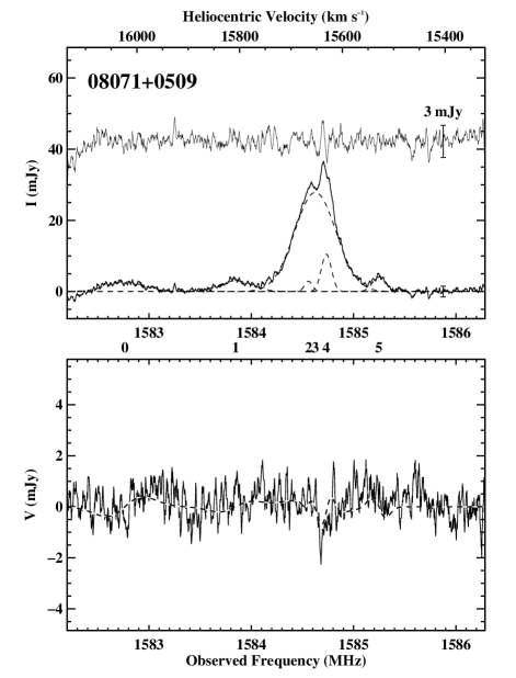
(a) IRAS 08071+0509: Zeeman splitting non-detection.

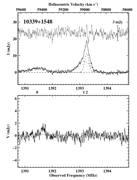
(b) IRAS F10339+1548: Zeeman splitting non-detection.

Each sub-figure shows Stokes $I$ and $V$ spectra in two panels. Sub-figures (a), (b), and (c) show non-detections of Zeeman splitting. Sub-figures (d), (e), and (f) are considered marginal Zeeman splitting detections. The remaining sub-figures are new Stokes $V$ detections. In each sub-figure, the top panel shows the Stokes $I$ spectrum for each source. The flux density is defined as the sum of the orthogonal polarization, $I=RHCP+LHCP$, rather than the average. The data are shown by the solid line. The dashed lines are Gaussian components used to fit the overall profile. The thin solid line shows the residuals of the fits, expanded by a factor of three. The bottom panel in each sub-figure shows the Stokes $V$ profile. The data are indicated by the solid line. The fit, produced using the Gaussians in the top panel as inputs, is shown with a dashed line.

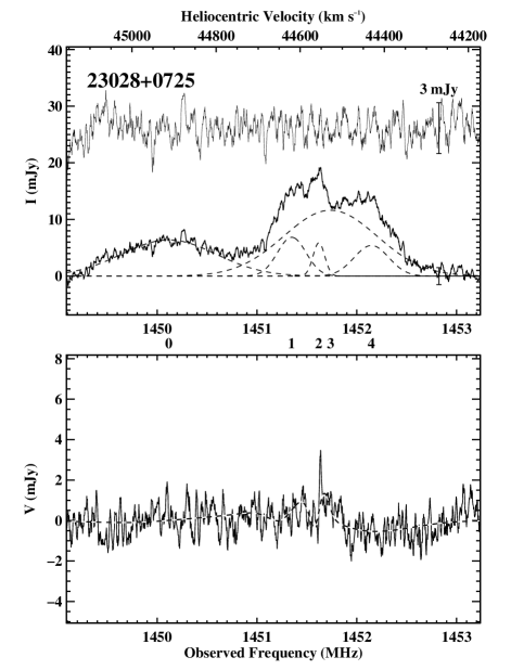
(c) IRAS F23028+0725: Zeeman splitting non-detection.

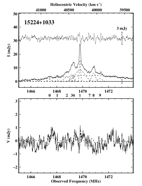
(d) IRAS F15224+1033: Marginal detection of Zeeman splitting.

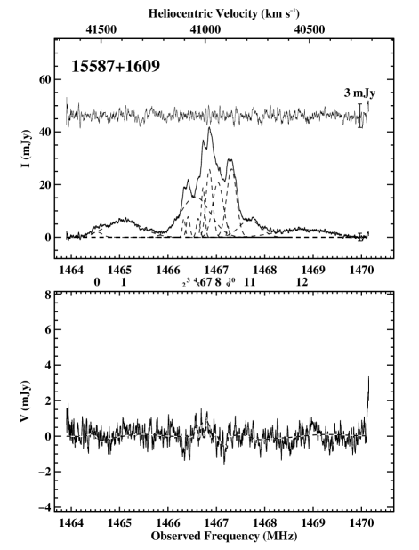
(e) IRAS F15587+1609: Marginal detection of Zeeman splitting.

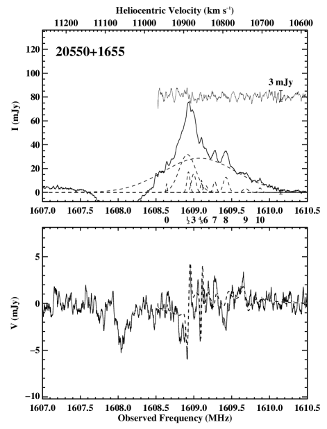
(f) IRAS F20550+1655: Marginal detection of Zeeman splitting.

(continued)

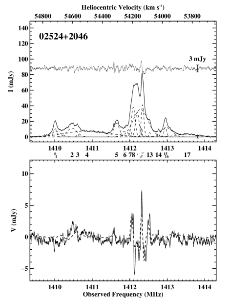
(g) IRAS F02524+2046: Zeeman splitting detection.

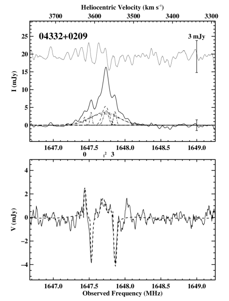
(h) IRAS F04332+0209: Zeeman splitting detection. Instead of showing fits to Stokes $I$, the $RHCP$ (dashed) and $LHCP$ (dash-dot) are plotted in the top panel, and $RHCP-LHCP$ for the fitted Gaussian is shown in the bottom panel.

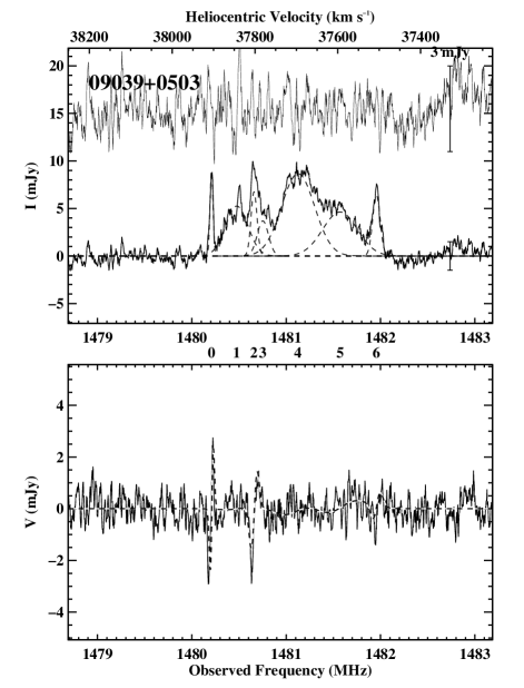
(i) IRAS F09039+0503: Zeeman splitting detection.

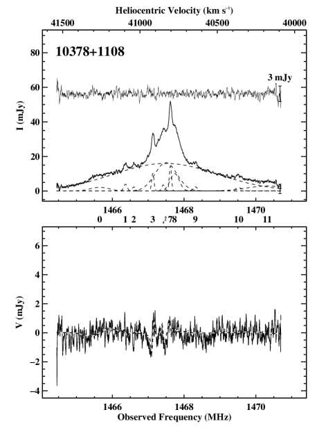
(j) IRAS F10378+1108: Zeeman splitting detection.

(continued)

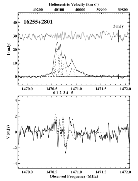
(k) IRAS F16255+2801: Zeeman splitting detection.

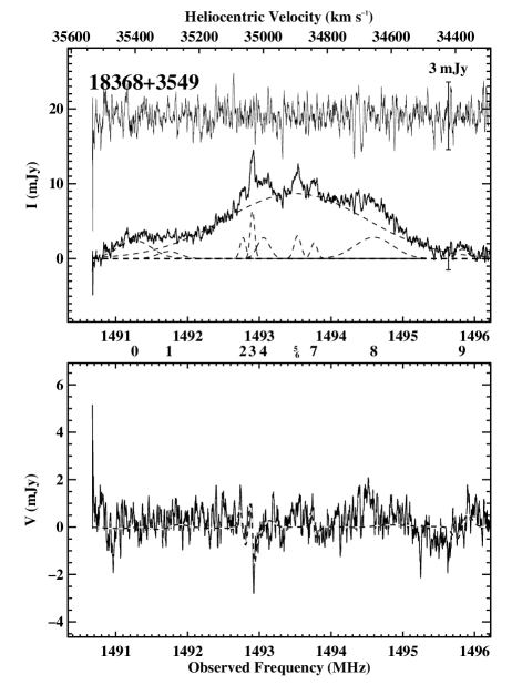
(l) IRAS F18368+3549: Zeeman splitting detection.

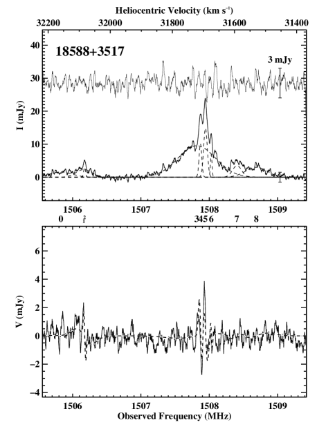
(m) IRAS F18588+3517: Zeeman splitting detection.

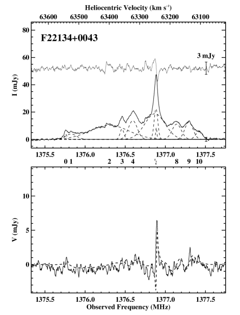
(n) IRAS F22134+0043: Zeeman splitting detection.

Figure 5.— (continued)

IRAS F00509+1225: This OHM was first reported by Bottinelli et al. (1990), with $\log(L_{\rm OH}/L_{\odot})=1.78$, but has no published spectrum. Given the reported redshift $z_{\odot}=0.060875$, the likely luminosity distance they used is 243 Mpc. For the (Hinshaw et al., 2009) cosmology, the luminosity distance at this redshift is 271 Mpc, implying an isotropic luminosity of $\log(L_{\rm OH}/L_{\odot})=1.88$. At this redshift, maser emission should be expected near 1571 MHz. While the composite spectrum has features near this frequency, those features completely disappear or even appear as absorption in bootstrap resampling, suggesting they are instead due to interference from GPS L2 that is centered at 1575.42 MHz. The rms error is 5 mJy, so we place an upper limit $\log(L_{\rm OH}/L_{\odot})\leq 1.82$ on the isotropic luminosity of OHM emission, weakly suggesting that this source is not actually an OHM.

IRAS F03056+2034: Bottinelli et al. (1990) reported this OHM with a an isotropic luminosity of $\log(L_{\rm OH}/L_{\odot})=1.28$. Located at a redshift of $z=0.027369$, the expected maser emission is in a frequency range dominated by spiky interference likely from the Iridium satellite, so much so that even the median composite spectrum had an rms of 15 mJy. From this, we place an upper limit on the isotropic luminosity of the OHM emission that we could detect of $\log(L_{\rm OH}/L_{\odot})\leq 1.60$. This is larger than the previously reported value, so the non-detection is unsurprising.

IRAS F11069+2711: No spectrum of this OHM is available, nor are there any published properties. It was listed as a megamaser by Baan et al. (1998). There is spiky interference in our spectra, so we took the median of shorter spectra to produce the total spectrum. Baan et al. (1998) assumed a redshift for this source of of $z=0.0703$, which places the expected frequency for OHM emission at 1557.8 MHz. There is a roughly 5 mJy feature centered around 1557.5 MHz, but this is likely due to terrestrial interference, as it appears intermittently in spectra both on and off source. A more recent redshift measure by Lawrence et al. (1999) puts the galaxy at a redshift of $z=0.072971$, shifting the expected frequency for OHM emission to 1554 MHz. At this frequency, there is nothing resembling emission. Outside of the interference at 1557.5 MHz, there is an rms error of 2.3 mJy, which we use to place an upper limit on the OHM luminosity of $\log(L_{\rm OH}/L_{\odot})<1.65$.

IRAS F13451+1232: With a 5.4 Jy continuum flux at 1.4 GHz, this OHM is the strongest continuum source in our sample. A tentative OH detection was claimed by Dickey et al. (1990), who reported a flux of 1.7 mJy and an isotropic luminosity of $\log(L_{\rm OH}/L_{\odot})$ = 2.38. While most spectra in our sample have rms errors of order 1 mJy, the combination of strong continuum emission and interference in the spectrum for this source resulted in an rms error of $\sim 20$ mJy, so we can neither confirm nor refute this tentative detection.

IRAS F15233+0533: Baan et al. (1998) listed this as a megamaser, but no published spectrum or properties are available. At a redshift of $z=0.054064$, OHM emission is expected at 1581.8 MHz, which is near interference from GPS L2 located at 1575.42 MHz. There are no features in the final spectrum that are clearly persistent. Bootstrap resampling of the 4-minute spectra shows that features in the composite spectrum are not clearly persistent. With an rms error of 20 mJy, we place an upper limit of $\log(L_{\rm OH}/L_{\odot})<2.33$ for OHM emission from this galaxy.

IRAS F17526+3253: This source was first observed for OH emission by Garwood et al. (1987), who reported a non-detection with a spectrum that had 1.0 mJy rms noise, which corresponds to an upper limit on the isotropic luminosity of $\log(L_{\rm OH}/L_{\odot})<0.60$ for the chosen cosmology. An OHM was reported two years later by Martin et al. (1989), with an isotropic luminosity of $\log(L_{\rm OH}/L_{\odot})=0.99$, but no accompanying flux or spectrum was published. In our spectrum, interference from the Iridium satellite is severe. After combining the median spectra, the rms error is $\sim$10 mJy, so we do not detect OHM emission, and cannot place any useful new limit on OHM emission from this galaxy.

IRAS F20491+1846: This OHM was first reported by Bottinelli et al. (1989). There is no published flux, and the published isotropic luminosity is $\log(L_{\rm OH}/L_{\odot})=1.09$ at a redshift of 0.0290. Even looking at the median spectrum, spiky interference from the Iridium satellite dominates. With roughly 30 mJy rms error in the spectrum, the upper limit on the isotropic luminosity is $\log(L_{\rm OH}/L_{\odot})=1.96$, well above the reported luminosity.

IRAS F23135+2517: Interference from the Iridium satellite is present in the spectrum for this source. Combining the median of the median spectra, the rms error in the spectrum is $\sim 20$ mJy. Mirabel & Sanders (1987) reported a flux of 2.4 mJy for this source, corresponding to 4.8 mJy for our definition, so the OHM is not detected.

5.1.4 Ambiguous Stokes $I$ detections

IRAS F15250+3608: This OHM was reported in an IAU Circular by Bottinelli et al. (1987) to have an isotropic luminosity of $\log(L_{\rm OH}/L_{\odot})=2.58$. At a redshift of $z=0.0554$, OHM emission is expected at roughly 1580 MHZ, near interference from GPS L2 at 1575.42 MHz. There is at least one persistent feature near 1581 MHz, and perhaps more than one, but these are mixed among ripply interference that clearly fluctuates. It is therefore not possible to reliably estimate any of the OHM properties.

IRAS F23050+0359: This OHM has no published spectrum, or properties, but was listed as an OH megamaser by Baan et al. (1998). It is located at a redshift of 0.0474, putting the OH lines at a frequency near a strong source of interference, likely ringing from GPS L2, that contaminates the low frequency side of the spectrum. Even so, there appears to be a detection of the 1667 MHz line, and possibly the 1665 MHz line. The Stokes $V$ spectrum has significant rippling, which prevents any possible Zeeman splitting detection or placement of useful limits on magnetic fields in this OHM.

IRAS F23365+3604: Bottinelli et al. (1990) reported this OHM to have an isotropic luminosity of $\log(L_{\rm OH}/L_{\odot})=2.44$, but did not publish any other properties of the source. Subsequently, Baan et al. (1992) cited the upper limit on the isotropic luminosity of the 1667 MHz line to be $\log(L_{\rm OH}/L_{\odot})<1.93$, assuming a 100 $\;{\rm km\;s}^{-1}$ linewidth. Darling & Giovanelli (2002a) considered the source suspect. The source is at a redshift of 0.064531, which puts the 1667 MHz OH line at a frequency of 1566.3 MHz. The composite spectrum created by taking the mean of individual 1-second spectra shows significant broadband interference. Median combination of individual spectra to create a composite removes most features, leaving what appears to be a reasonably flat spectrum with broad, low SNR emission from 1566.5–1568 MHz, plausibly close to the expected frequency of the OH line, and would correspond to an isotropic luminosity of $\log(L_{\rm OH}/L_{\odot})=2.56$. Spectra of the 1612 MHz line of IRAS F01417+1651, another source observed in this survey, spanned the frequency range 1566.1–1572.3 MHz. Examination of these spectra showed features of comparable shape and intensity to those that were appeared in the median composite spectrum for IRAS F23365+3604, strongly suggesting that the apparent emission is actually interference.

5.1.5 Stokes $V$ non-detections

For the sources described in this section, maser emission was detected, but due to low signal-to-noise in the Stokes $I$ and Stokes $V$ spectra, it was not possible to identify any features in the Stokes $V$ as being associated with features in the Stokes $I$ spectrum. For the majority of sources, we do not present the spectrum, instead providing a reference where a published spectrum can be found. Exceptions are made for three sources, IRAS F08071+0509, IRAS F10339+1548, and IRAS F23028+0725. For IRAS F08071+0509, no Stokes $I$ spectrum exists in the literature. In the case of IRAS F10339+1548, our data provided an improvement over the existing Stokes $I$ data, allowing determination of the hyperfine ratio, which is defined as the ratio of the flux in the 1667 MHz main line to the flux in the 1665 MHz main line, or $R_{H}=F_{1667}/F_{1665}$. IRAS F23028+0725 is included as an example of a source where our fitting routine reported marginally significant detection of Zeeman splitting that we do not find credible.

Where possible, we estimate an upper limit to the magnetic field strength associated with the masing regions. Following Troland & Heiles (1982), the upper limit is taken to be the fitted field strength plus three times the error associated with the fitted field. Most OHMs are fit with multiple Gaussian components; for sources where an upper limit is reported, the value is that of the Gaussian component with the lowest associated error that appeared to be real. This is based on the shape and strength of features in the Stokes $I$ spectrum, and the structure and amplitude of noise in the Stokes $V$ spectrum. For example, limits associated with Gaussians fit to wide features in spectra are not reported, as they are likely bandpass features. We consider only one digit in these upper limits to be significant, but reported two digits for sources with upper limits between 10–20 mG.

IRAS F01562+2528: This OHM, reported in DG02, has three broad, blended features, one of which is at the expected frequency of the redshifted 1665 MHz line. Despite the well-detected signal in Stokes $I$, there are no features in the Stokes $V$ spectrum that look promising. Given the absence of any narrow structures, it is not possible to constrain the magnetic field in any meaningful way.

IRAS 03521+0028: DG02 discovered this OHM, noting the excellent agreement between the peak of the 1667 MHz emission and the published optical redshift, as well as marginal detection of the 1665 MHz line. Our spectrum has an additional narrow feature at 1448.3 MHz not seen in the DG02 observations. Examination of multiple spectra for different objects that have observations in this frequency range show that this new, narrow feature is interference. No features in the Stokes $V$ spectrum can be identified as associated with the astrophysical Stokes $I$ emission, and the lack of bright, narrow emission prevents placing a useful limit on the magnetic field in this OHM.

IRAS F03566+1647: This OHM was reported by DG02, and features broad, low amplitude emission. The Stokes $V$ spectrum has no apparent features, and the broad Stokes $I$ features do not provide useful limits on the magnetic fields in this source.

IRAS F04121+0223: The spectrum for this OHM discovered by DG01 contains one narrow component centered at 1485.20 MHz and one broad feature centered at 1486.04 MHz. The Stokes $V$ spectrum does not show any features associated with the Stokes $I$ emission, and we place an upper limit of 40 mG on the magnitude of magnetic fields associated with the narrow emission in this OHM.

IRAS 06487+2208: DG00 reported this OHM, featuring two main 1667 MHz peaks centered at 1457.7 MHz and 1458.3 MHz, and weak, corresponding 1665 MHz emission. There is a great deal of structure in the Stokes $I$ spectrum, requiring a total of nine Gaussians to produce a good fit. The Stokes $V$ spectrum features 1 mJy ripples, but no apparent Zeeman splitting signature. We place an upper limit of 10 mG on the magnetic field associated with the narrow emission at 1457.7 MHz as well as the broader emission centered at 1458.3 MHz.

IRAS 07163+0817: This OHM discovered by DG01 features three distinct 1667 MHz peaks, one of which is centered at 1501.3 MHz and is about twice as bright as the other two peaks. The Stokes $V$ spectrum does not have any notable features, and we place an upper limit of 20 mG on the magnitude of a magnetic field associated with the narrow line at 1501.3 MHz.

IRAS 07572+0533: Only one broad feature can be distinguished for this OHM discovered by DG01. They noted an apparent second OH line offset blueward from the main feature by 400 $\;{\rm km\;s}^{-1}$, but we do not confidently detect this. Without any narrower lines, it is not possible to place useful limits on the magnetic fields in this source.

IRAS F07556+2859: This OHM was discovered by Willett (2012), and will be discussed in more detail in a future work by Willett, Darling, Kent, & Braatz. The Stokes $I$ spectrum features broad, blended 1667 MHz emission and weak 1665 MHz emission. Without any distinct narrow emission, we do not place any limits on magnetic fields in this OHM.

IRAS F08071+0509: Bottinelli et al. (1989) reported this OHM with $\log(L_{\rm OH}/L_{\odot})=2.25$, but did not publish a spectrum or the flux of the 1667 MHz line. Baan et al. (1998) classified it as a composite AGN/starburst in a survey to optically classify megamaser galaxies. We clearly detect the maser, but there are no circular polarization features, as can be seen in Figure 5(a). The flux of the 1667 MHz line is 35 mJy, and the isotropic luminosity is $\log(L_{\rm OH}/L_{\odot})=2.12$. For their likely choice of cosmology, this would correspond to $\log(L_{\rm OH}/L_{\odot})=2.03$, which is roughly 70% less luminous than they reported. It is not possible to identify Zeeman splitting in the Stokes $V$ spectrum. There is a large dip in the Stokes $V$ spectrum at the location of emission, but similar dips appear elsewhere in the spectrum. The upper limit on the magnetic field associated with Gaussian 4, which is a bright, relatively narrow, feature located near the peak of emission, is 20 mG. The rest of the parameters used to fit emission are shown in Table 2.

Table 2IRAS F08071$+$0509 Gaussian Fit Parameters

	$S$	$\nu$	$\Delta\nu$	$v_{\odot}$	$B_{\parallel}$
Gaussian	(mJy)	(MHz)	(MHz)	(km s-1)	(mG)
(1)	(2)	(3)	(4)	(5)	(6)
0	$\phantom{8}2.74\pm 0.20$	$1582.7638\pm 0.0143$	$0.4223\pm 0.0377$	$16023.2$	$-89.27\pm 29.37$
1	$\phantom{8}3.03\pm 0.21$	$1583.8481\pm 0.0130$	$0.3814\pm 0.0338$	$15807.0$	$-38.07\pm 25.31$
2	$\phantom{8}2.90\pm 0.91$	$1584.5591\pm 0.0023$	$0.0902\pm 0.0082$	$15665.4$	$\phantom{}-8.82\pm 13.27$
3	$27.84\pm 0.80$	$1584.6262\pm 0.0067$	$0.4756\pm 0.0243$	$15652.1$	$\phantom{-}\phantom{8}6.26\pm 3.23\phantom{8}$
4	$10.49\pm 0.80$	$1584.7340\pm 0.0024$	$0.1168\pm 0.0082$	$15630.6$	$\phantom{}-9.77\pm 4.19\phantom{8}$
5	$\phantom{8}4.10\pm 0.32$	$1585.2492\pm 0.0058$	$0.1532\pm 0.0142$	$15528.1$	$\phantom{-}23.32\pm 11.83$

IRAS F08201+2801: DG01 discovered this OHM, which features broad 1667 MHz emission, and low flux emission redward of the main 1667 MHz features, which DG01 suggested could be either 1665 MHz emission or high velocity 1667 MHz emission. Overall, it has rich enough structure that ten Gaussian components are needed to produce a reasonable fit to the full 1665/1667 MHz emission. The Stokes $V$ spectrum has little in the way of structured noise, and shows no compelling features. We place an upper limit of 20 mG on fields in this OHM.

IRAS F08279+0956: This OHM was reported by DG01. It features two broad, blended 1667 MHz features in the Stokes $I$ spectrum, but at such low signal-to-noise that even with minimal structured noise in the Stokes $V$ spectrum, it is not possible to place any useful constraint on magnetic fields associated with this OHM.

IRAS F08449+2332: The maser emission of this OHM discovered by DG01 overlaps with the same 1448.3 MHz interference that appeared in the spectrum of IRAS F03521+0028. As such, no magnetic field is detected, nor is it possible to place any useful limit on magnetic field properties.

IRAS F08474+1813: DG01 discovered this OHM, which has a roughly 4 mJy peak flux density, and three broad emission features that are distinguishable. The low flux density and broad lines means the Stokes $V$ observations do not provide any useful limits on magnetic fields in this OHM.

IRAS F09531+1430: This OHM was discovered by DG01, and the spectrum has two moderately narrow, well separated peaks atop a broad region of emission. Though no field is detected for either of the narrow features, we may place an upper limit of 30 mG on magnetic fields associated with either peak.

IRAS F09539+0857: This OHM, discovered by DG01, has broad, blended 1665/1667 MHz emission and rich structure. We use nine Gaussian components to the total 1665/1667 MHz emission, including multiple narrower features, and achieve an adequate fit. The Stokes V spectrum has reasonably well behaved noise, but there are no suggestions of Zeeman splitting. The upper limit on the magnetic field associated with multiple narrow Gaussians fit to peaks in the emission is 20 mG.

IRAS F10035+2740: There are two broad, low signal-to-noise features in the spectrum of this OHM, which was discovered by DG02. These broad features do not provide a useful limit on the magnetic fields in the masing region of this galaxy.

IRAS F10339+1548: The OHM, discovered by DG01, is clearly detected at 1667 MHz. Weak 1665 MHz emission is also visible in our spectrum, shown in Figure 5(b), while standing waves frustrated the detection of the 1665 MHz emission in the DG01 observations. We fit one Gaussian to the 1665 MHz emission, and one broad and one narrow Gaussian to the 1667 MHz emission, which are shown in Table 3. From the Gaussian, we compute a hyperfine ratio $R_{H}=21$. The peak of emission is fit by Gaussian 2, and with well behaved noise in the Stokes $V$ spectrum, we can place an upper limit of 20 mG on magnetic fields in this source.

Table 3IRAS F10339$+$1548 Gaussian Fit Parameters

	$S$	$\nu$	$\Delta\nu$	$v_{\odot}$	$B_{\parallel}$
Gaussian	(mJy)	(MHz)	(MHz)	(km s-1)	(mG)
(1)	(2)	(3)	(4)	(5)	(6)
0	$\phantom{8}2.39\pm 0.14$	$1391.4459\pm 0.0198$	$0.7723\pm 0.0550$	$59446.6$	$-136.05\pm 49.28$
1	$\phantom{8}6.69\pm 0.41$	$1393.1475\pm 0.0101$	$0.5373\pm 0.0203$	$59007.8$	$\phantom{}-50.12\pm 15.57$
2	$11.26\pm 0.45$	$1393.2540\pm 0.0025$	$0.1841\pm 0.0079$	$58980.4$	$\phantom{}\phantom{}-2.35\pm 5.41\phantom{8}$

IRAS F11028+3130: The spectrum for this OHM, reported by DG01, has two broad features, one corresponding to the 1667 MHz line and one to the 1665 MHz line, and a low amplitude 1667 MHz feature on the redward side of the broad 1667 MHz emission. Given the low snr, it is not possible to place any useful limit on the magnetic field strength for this source.

IRAS F11180+1623: DG02 discovered this OHM, which has only one easily identified emission component with a peak flux density of roughly 4 mJy. With such a weak signal, no useful limit may be placed on the presence of magnetic fields in this galaxy.

IRAS F11524+1058: This OHM was discovered by DG01. It has broad emission, which we fit with four reasonably broad Gaussians. The lack of distinguishable narrow spectral features prevents placing useful limits on the magnetic field in this galaxy.

IRAS F12005+0009: Though this OHM, discovered by DG02, has a peak flux density of only 9 mJy, it features multiple distinguishable emission components, including one relatively narrow peak centered on a broad hump. The fits to the Stokes $V$ spectrum yields a 3$\sigma$ claimed detection for a 21 mG field associated with the narrow peak. Unfortunately, the Stokes $V$ spectrum for this source includes many narrow ripples of the same characteristic size as the narrow feature, and shifting the Stokes $I$ and $V$ spectra relative to each other reveals many shifts that produce a claimed magnetic field detection. We place an upper limit of 40 mG on magnetic fields associated with masing clouds in this galaxy.

IRAS F12018+1941: Only one broad feature may be distinguished in the spectrum of this OHM discovered by Martin et al. (1988b). It is not possible to place a useful limit on the magnetic field in this OHM.

IRAS F12162+1047: DG02 reported this OHM, which has broad, low flux density emission. The Stokes $I$ spectrum may be adequately fit with two broad Gaussians, but does not allow any useful limit to be placed on magnetic fields in this galaxy.

IRAS F12243-0036: Martin et al. (1988b) discovered this OH kilomaser, which has apparent absorption bracketing the maser emission. The overall profile is complicated, and may only be adequately fit. Nevertheless, there are a few narrow emission features in the spectrum, and one that is aligned with a feature in the Stokes $V$ spectrum. The fit to Stokes $V$ suggests a field detection, but shifts between Stokes $I$ and $V$ also produce claimed fields. We place an upper limit of 20 mG on the magnetic field associated with this maser.

IRAS F12549+2403: DG02 discovered this OHM, which has two broad, 1667 MHz emission components and marginally detected 1665 MHz emission in the Stokes $I$ spectrum. No useful limit may be placed on the magnetic field in this galaxy.

IRAS F13126+2453: This source is classified as an OH absorber and kilomaser. Darling & Giovanelli (2002a) reported that no published spectrum exists, but a published spectrum is available in Schmelz et al. (1986) under the designation IC 860, so the spectrum is not provided again here. The absorption in both the 1665 and 1667 MHz lines is clearly detected, as well as emission at the wings of the absorption features. For the absorption alone, the hyperfine ratio is $R_{H}=1.27\pm 0.18$, while for the emission, we find a hyperfine ratio of $R_{H}=1.3\pm 0.36$, where the errors are based on reported errors to Gaussian fits to the spectra. Both are consistent with OH in local thermodynamic equilibrium.

The Stokes $V$ spectrum features bandpass structure on scales comparable in width to features in the Stokes $I$ spectrum, leading to claimed fields with magnitudes of $\sim$30–40 mG associated with the absorption features. We do not consider these claims to be reliable. The noise in the vicinity of the emission components has less structure than in the regions of absorption, but there is no sign of Zeeman splitting. In the emission regions, we place an upper limit of 30 mG on the magnitude of magnetic fields.

IRAS F13218+0552: Among broad emission in the spectrum of this OHM discovered by DG02, there is one narrow feature at 1384.8 MHz. The Stokes $V$ spectrum has well-behaved noise in the vicinity of the narrow emission seen in Stokes $I$, but there is no sign of Zeeman splitting. We place an upper limit of 50 mG on the magnetic field associated with the masing region in this source.

IRAS F14043+0624: This OHM, discovered by DG02, has an asymmetric 1667 MHz emission profile best fit by one narrow and one moderately wide Gaussian, along with one broad, weak 1665 MHz line. No magnetic field is detected, and we place an upper limit of 40 mG on magnetic fields in this galaxy.

IRAS F14059+2000: DG02 discovered this OHM, which has bright 1667 MHz emission that is well fit by one very broad Gaussian and one moderately broad Gaussian, and 1665 MHz emission that blends with the red wing of 1667 MHz emission. No Zeeman splitting is apparent in the Stokes $V$ spectrum, and we place an upper limit of 20 mG on the magnitude of magnetic fields associated with this OHM.

IRAS F14553+1245: There is one relatively narrow, low SNR feature in the spectrum of this OHM. It was discovered by DG02, and like them, we do not see a clear 1665 MHz component in the spectrum. The Stokes $V$ spectrum is nearly featureless, and we place an upper limit of 60 mG on magnetic fields associated with this OHM.

IRAS F14586+1432: This OHM, discovered by DG02, has a rich, blended spectrum, spread over more than 5 MHz. Despite this richness, there are few identifiable narrow features in the spectrum. Fits to Stokes $V$ provide claimed magnetic fields, but so too do fits when the Stokes $V$ is shifted relative to Stokes $I$, thanks to a number of ripples in the Stokes $V$ spectrum. This is regarded as a non-detection, and it is difficult to provide a meaningful upper limit on magnetic fields in this galaxy.

IRAS F15107+0724: Bottinelli et al. (1986) discovered this OHM, and a spectrum is available in Baan et al. (1987) and Martin et al. (1988a). The 1667 MHz emission has a dual-peaked structure, which is closely matched by the 1665 MHz emission. A total of six Gaussian components are needed to fit the Stokes $I$ spectrum, four of which are narrow. While no Zeeman splitting is seen in the Stokes $V$ spectrum, each of the narrow components is consistent with an upper limit of 12–15 mG to the magnitude of magnetic fields in this OHM.

IRAS F16100+2527: DG01 discovered this OHM, which has emission made up of a broad 1667 MHz line with a marginally distinct peak, and a similarly broad and well separated 1665 MHz line. The 1667 MHz emission can be reasonably fit with one wide and one narrow Gaussian. The nearly 6 mJy narrow feature provides a 40 mG upper limit on the magnitude of magnetic fields in this OHM.

IRAS F16300+1558: This OHM was discovered by DG00, but RFI plagued their observations. Our spectra combined by taking the median do not have serious narrow RFI, but do feature significant bandpass structure. Like DG00, we do not clearly detect the 1665 MHz line. Structure of unclear origin in both the Stokes $I$ and $V$ spectra prevents placing any useful limits on magnetic fields in this OHM.

IRAS F17161+2006: The 1667 MHz emission from this source, discovered by DG02, has a peak flux density of less than 10 mJy. Four Gaussians are required to reasonably fit the profile, three for the 1667 MHz emission and one for the broad 1665 MHz emission. One of the 1667 MHz components is reasonably narrow, and provides an upper limit of 60 mG on the magnitude of the magnetic field associated with this OHM.

IRAS F17207-0014: Bottinelli et al. (1985) reported this OHM, which has a spectrum with strong interference from GLONAS. Despite the interference, the maser is still clearly detected, as interference is negligible at frequencies lower than about 1601 MHz, based on inspection of individual spectra used to create the composite spectrum. Comparison of previously published spectra for the OHM in IRAS F17207-0014 (Martin et al., 1989; Momjian et al., 2006), as well as with spectra of other sourcing overlapping in frequency, confirms that the features below 1600 MHz are maser emission rather than interference. The Stokes $I$ profile is bright, but there are no distinct peaks in the emission. Moreover, the Stokes $V$ spectrum has significant broadband structure. While interference below 1601 MHz is mild compared to that above 1601 MHz, it still makes it difficult to detect Zeeman splitting in this source or place useful limits.

IRAS F17539+2935: This OHM, discovered by DG00, is only marginally detected, with a peak flux density of just over 1 mJy. The SNR is insufficient to detect magnetic fields or place any useful upper limits.

IRAS 20248+1734: While this OHM, discovered by DG00, is clearly detected, the spectrum for this OHM features standing waves that complicate fitting and identification of real emission, and it is not possible to detect Zeeman splitting or place useful limits on magnetic fields in this galaxy.

IRAS 20286+1846: DG00 discovered this OHM, which has extremely broad, blended 1665/1667 MHz masing lines. To fit the total profile adequately requires nine components, three of which are relatively narrow. No Zeeman splitting is detected for any of the three narrow components, but we place an upper limit of 20 mG on magnetic fields in this OHM.

IRAS 20450+2140: This OHM was reported in DG00. The Stokes $I$ spectrum shows two blended 1667 MHz emission components, adequately fit by two Gaussians. The width of the fitted Gaussians is too large to place any useful limits on magnetic fields in this galaxy.

IRAS 21077+3358: DG00 reported this OHM, which has broad 1667 MHz that possibly blends with its 1665 MHz component. It is not possible to clearly distinguish any narrow features in the spectrum, or place any useful limits on magnetic fields in this galaxy.

IRAS 21272+2514: The spectrum of this OHM, discovered by DG00, is rich in structure, and very broad. It is not possible to clearly distinguish the 1665 MHz and 1667 MHz lines. The full spectrum is reasonably well-fit by ten Gaussians, six of which are moderately narrow. No magnetic fields are detected, and we place an upper limit of 20 mG on magnetic fields in the masing region in this galaxy.

IRAS 22055+3024: The spectrum of this OHM, reported in DG01, has moderately broad 1667 MHz emission and a distinct 1665 MHz line. The 1667 MHz features are well fit with a wide base and two narrow Gaussians. There is some rippling structure in the Stokes $V$ in the vicinity of the narrow lines, but the noise is well enough behaved to provide a 30 mG upper limit on magnetic fields in this OHM.

IRAS F22116+0437: This OHM was detected by DG00. Though it is re-detected here, it is insufficiently bright to place any useful limit on magnetic fields.

IRAS F23019+3405: Emission from this OHM, reported in DG01, is quite narrow, with a FWHM of roughly $60\;{\rm km\;s}^{-1}$. It nevertheless appears to have a bi-peaked structure, though higher SNR spectra would be required to confirm this. No Zeeman splitting is apparent in the Stokes $V$ spectrum, but we are able to place an upper limit of 30 mG on magnetic fields in this OHM.

IRAS F23028+0725: DG01 reported this OHM, which has a broad 1667 MHz emission that blends with a clear 1665 MHz component. Five Gaussians are needed to adequately fit the combined 1665/1667 MHz emission, shown in Figure 5(c). Gaussian components 1 and 2 are moderately narrow, and produce fits with reported $\sim 3\sigma$ magnetic fields having magnitudes of $\sim 40$ mG. The spectrum is not convincing to the eye, however, and shifting the Stokes $I$ and $V$ relative to each other confirms this, as non-zero shifts produce stronger fits to the Stokes $V$ spectrum, as seen in Figure 1. For this reason, it is difficult to place useful limits on magnetic fields in this galaxy.

IRAS F23129+2548: Emission in this OHM, reported in DG01, is broad, and the 1665 MHz and 1667 MHz lines are blended. The total spectrum is well fit with six Gaussians, though only one is narrow. Zeeman splitting is not observed, but noise in the Stokes $V$ spectrum is well enough behaved to provide an upper limit of 50 mG on magnetic fields in this OHM.

IRAS F23199+0123: This OHM was reported by DG01. The 1667 MHz emission is broad, and has a peak flux density of only 3 mJy. It is not clear if 1665 MHz emission is detected. Given the low flux density, no meaningful limit may be placed on magnetic fields in this OHM.

IRAS F23234+0946: DG01 discovered this OHM. It has broad 1667 MHz emission with an apparent blue tail and 1665 MHz line. Four total Gaussians adequately fit the spectrum, one of which is narrow and near the peak of 1667 MHz emission. No Zeeman splitting is detected, but the narrow feature provides an upper limit of 50 mG on the magnitude of magnetic fields in this OHM.

5.1.6 Marginal Stokes $V$ detections

The three sources presented in this section, IRAS F15224+1033, IRAS F15587+1609, and IRAS F20550+1655, all have features in their Stokes $V$ spectra consistent with Zeeman splitting. They also have Stokes $V$ structure that does not appear to be associated with any maser emission. For this reason, they are considered only “marginal” detections. In Table 4, Table 5, and Table 6, the fitted features that are consistent with detections of Zeeman splitting are highlighted with bold text.

IRAS F15224+1033: This OHM, discovered by DG01, has a rich, wide Stokes $I$ spectrum, and a fairly noisy Stokes $V$ spectrum, shown in Figure 5(d). Any 1665 MHz emission that might be present is blended with the broad 1667 MHz emission. The features of the OHM have not changed significantly since DG01. The complexity requires nine Gaussians to adequately fit, and even then, the residuals show structure that coincides with the two brightest features, which are fit by Gaussian components 3, 4, and 6. The full fits are shown in Table 4. At the same frequency as Gaussian 6, there is a weak feature in the Stokes $V$ spectrum, with a peak-to-trough amplitude only marginally larger than that of others in the spectrum. The fits regard this as a 3.9$\sigma$ detection of a -8.3 mG magnetic field. There is also a marginally significant fit associated with Gaussian 4, with a reported field of -26.7$\pm$8.5 mG, but the fitted structure in Stokes $V$ does not appear markedly different to eye than other features in the spectrum. Altogether, the structure in the Stokes $V$ spectrum that is apparently unassociated with features in the Stokes $I$ spectrum, and the marginal appearance of the fitted features, limits our confidence in the two reported fields.

Table 4IRAS F15224$+$1033 Gaussian Fit Parameters

	$S$	$\nu$	$\Delta\nu$	$v_{\odot}$	$B_{\parallel}$
Gaussian	(mJy)	(MHz)	(MHz)	(km s-1)	(mG)
(1)	(2)	(3)	(4)	(5)	(6)
0	$\phantom{8}1.35\pm 0.18$	$1467.4444\pm 0.0212$	$0.3575\pm 0.0593$	$40841.7$	$-179.44\pm 43.83$
1	$\phantom{8}1.11\pm 0.23$	$1468.0327\pm 0.0197$	$0.2063\pm 0.0520$	$40705.2$	$\phantom{-}\phantom{8}52.26\pm 40.79$
2	$\phantom{8}3.25\pm 0.19$	$1468.7777\pm 0.0272$	$0.4532\pm 0.0595$	$40532.5$	$\phantom{}-40.08\pm 23.32$
3	$\phantom{8}5.36\pm 0.69$	$1469.1573\pm 0.0293$	$0.2430\pm 0.0619$	$40444.5$	$\phantom{}-14.76\pm 10.59$
4	$\phantom{8}4.75\pm 1.78$	$1469.3149\pm 0.0118$	$0.1446\pm 0.0255$	$40408.0$	$\phantom{}{\bf-26.62\pm 8.45}\phantom{8}$
5	$\phantom{8}8.30\pm 0.32$	$1469.7945\pm 0.0010$	$0.8947\pm 0.0029$	$40297.0$	$\phantom{}\phantom{}-0.09\pm 12.39$
6	$15.76\pm 0.22$	$1469.7968\pm 0.0094$	$0.1116\pm 0.0338$	$40296.5$	$\phantom{}\phantom{}{\bf-8.27\pm 2.13}\phantom{8}$
7	$\phantom{8}4.34\pm 0.29$	$1470.5376\pm 0.0686$	$6.3929\pm 0.4799$	$40125.2$	$\phantom{-}\phantom{8}86.82\pm 66.19$
8	$\phantom{8}6.07\pm 0.20$	$1470.8441\pm 0.0059$	$0.3314\pm 0.0156$	$40054.3$	$\phantom{-}\phantom{8}14.55\pm 9.88\phantom{8}$
9	$\phantom{8}2.09\pm 0.19$	$1471.3402\pm 0.0175$	$0.3661\pm 0.0478$	$39939.7$	$\phantom{}\phantom{}-8.39\pm 30.00$

IRAS F15587+1609: The spectrum of this OHM, reported in DG01, has a great deal of structure, with three distinct peaks, and many narrow features. Figure 5(e) shows our fits, and Table 5 lists the fits, which use eleven total Gaussians for the 1667 MHz emission, and two more for the 1665 MHz emission. In fitting the Stokes $V$ spectrum, there are three reported magnetic fields, associated with Gaussians 6, 7, and 8, and each is just above 3$\sigma$ claimed detections. These are three of the four brightest Gaussian components used, have similar reported values of $6.1\pm 2.0$, $7.5\pm 1.9$, and $12.2\pm 3.5$, respectively, and are contained within a roughly 100$\;{\rm km\;s}^{-1}$ range of velocities.

We regard this claimed magnetic field detection as marginal primarily because the fitted features do not look particularly compelling to the eye. Though there are noticeable dips in the Stokes $V$ spectrum near the same frequency as the brightest emission seen in the Stokes $V$, there are no features strongly resembling Zeeman splitting. Given the complex structure of the spectrum, shifting the Stokes $I$ and $V$ spectra relative to each other does not provide significant insight. The fits are of highest quality for no shift, but are of only slightly lower quality at a shift of 0.12 MHz, which is roughly the average of the frequency separation between Gaussian 5, 6, 7, and 8. Shifting the Stokes $I$ and $V$ by roughly 0.5 MHz relative to each other, corresponding to the separation between the central peak and the redward peak, also produces claimed fields, though they are also of lower quality than when no shift is applied. Taken together, we are not confident in these reported fields.

Table 5IRAS F15587$+$1609 Gaussian Fit Parameters

	$S$	$\nu$	$\Delta\nu$	$v_{\odot}$	$B_{\parallel}$
Gaussian	(mJy)	(MHz)	(MHz)	(km s-1)	(mG)
(1)	(2)	(3)	(4)	(5)	(6)
0	$\phantom{8}1.91\pm 0.28$	$1464.5345\pm 0.0130$	$0.2546\pm 0.0426$	$41117.9$	$\phantom{-}24.22\pm 16.49$
1	$\phantom{8}6.23\pm 0.14$	$1465.0808\pm 0.0129$	$0.8858\pm 0.0418$	$40990.7$	$-14.98\pm 9.46\phantom{8}$
2	$\phantom{8}7.08\pm 0.53$	$1466.3288\pm 0.0038$	$0.0686\pm 0.0076$	$41100.8$	$\phantom{-}\phantom{8}0.22\pm 4.21\phantom{8}$
3	$\phantom{8}7.75\pm 0.44$	$1466.4171\pm 0.0039$	$0.0862\pm 0.0100$	$41080.3$	$\phantom{-}\phantom{8}0.84\pm 4.32\phantom{8}$
4	$15.30\pm 0.61$	$1466.5661\pm 0.0337$	$0.7174\pm 0.0456$	$41045.7$	$\phantom{}-2.04\pm 6.34\phantom{8}$
5	$\phantom{8}7.06\pm 0.87$	$1466.6249\pm 0.0045$	$0.0843\pm 0.0122$	$41032.0$	$\phantom{-}12.01\pm 4.90\phantom{8}$
6	$18.78\pm 1.10$	$1466.7254\pm 0.0017$	$0.0847\pm 0.0053$	$41008.7$	$\phantom{-}\phantom{8}{\bf 6.12\pm 2.01}\phantom{8}$
7	$25.75\pm 3.70$	$1466.8546\pm 0.0036$	$0.1567\pm 0.0125$	$40978.6$	$\phantom{-}\phantom{8}{\bf 7.51\pm 1.94}\phantom{8}$
8	$20.80\pm 1.71$	$1467.0327\pm 0.0110$	$0.2574\pm 0.0458$	$40937.3$	$\phantom{-}{\bf 12.23\pm 3.48}\phantom{8}$
9	$\phantom{8}4.19\pm 0.64$	$1467.2375\pm 0.0026$	$0.0482\pm 0.0085$	$40889.7$	$\phantom{}-6.87\pm 5.47\phantom{8}$
10	$25.91\pm 1.29$	$1467.3137\pm 0.0076$	$0.2382\pm 0.0130$	$40872.0$	$\phantom{-}\phantom{8}0.60\pm 2.57\phantom{8}$
11	$\phantom{8}6.45\pm 0.17$	$1467.6886\pm 0.0156$	$0.5179\pm 0.0375$	$40785.0$	$\phantom{-}16.38\pm 13.72$
12	$\phantom{8}2.97\pm 0.13$	$1468.7666\pm 0.0258$	$1.2354\pm 0.0881$	$40535.0$	$-65.71\pm 40.91$

IRAS F20550+1655: This source was reported in an IAU Circular by Bottinelli et al. (1986), and a published spectrum is available in Baan et al. (1989), under the designation II Zw 96. Bottinelli et al. (1986) cite an isotropic luminosity of $\log(L_{\rm OH}/L_{\odot})=2.27$, and later sources use $\log(L_{\rm OH}/L_{\odot})=2.11$, in agreement with the value of $\log(L_{\rm OH}/L_{\odot})=2.13$ that we find. The spectrum, shown in Figure 5(f), suffers from interference in the 1602–1608.5 MHz part of the spectrum that is caused by the GLONAS satellite, including apparent absorption that just overlaps with redward side of the 1667 MHz line, redshifted to 1609 MHz. The interference is strongly linearly polarized, and also produces features in the Stokes $V$ spectrum. It is not clear if this interference appears beyond 1608.5 MHz in either the Stokes $I$ or $V$ spectra. Using eleven Gaussian components, provided in Table 6, to fit the emission blueward of 1608.5 MHz does an adequate job, and produces four magnetic field fits greater than $3\sigma$. Two of these are to wide components, and are not considered believable, but Gaussians 2 and 5 are narrow, and produce claimed fields of $-18.5\pm 2.4$ mG and $-17.4\pm 2.9$ mG, respectively, and also appear plausible examining the fits visually. The two Stokes $V$ features that are fit are the largest amplitude, from peak-to-trough, of any blueward of 1608.5 MHz, but there are two other dips that are not well accounted for. The interference at 1608 MHz is also shown, and is of comparable amplitude to the fitted features. Though it has a different shape, it casts doubt on the validity of the detection. Examining the variance of each channel of the Stokes $V$ spectrum shows a local maximum at 1608 MHz, corresponding to the interference, but has no apparent structure blueward of 1608.5 MHz, which suggests the fitted features in the Stokes $V$ spectrum are real. Given the conflicting evidence, we consider this a plausible magnetic field detection.

Table 6IRAS F20550$+$1655 Gaussian Fit Parameters

	$S$	$\nu$	$\Delta\nu$	$v_{\odot}$	$B_{\parallel}$
Gaussian	(mJy)	(MHz)	(MHz)	(km s-1)	(mG)
(1)	(2)	(3)	(4)	(5)	(6)
0	$\phantom{8}7.17\pm 1.14$	$1608.6408\pm 0.0014$	$0.0180\pm 0.0034$	$10942.9$	$\phantom{}-2.27\pm 3.20\phantom{8}$
1	$31.72\pm 1.10$	$1608.9151\pm 0.0050$	$0.2567\pm 0.0085$	$10890.0$	$-10.01\pm 2.91\phantom{8}$
2	$17.19\pm 1.06$	$1608.9286\pm 0.0019$	$0.0481\pm 0.0040$	$10887.4$	${\bf-18.53\pm 2.39}\phantom{8}$
3	$15.47\pm 1.50$	$1608.9974\pm 0.0024$	$0.0693\pm 0.0095$	$10874.1$	$\phantom{}-2.73\pm 3.13\phantom{8}$
4	$28.65\pm 1.32$	$1609.0765\pm 0.0016$	$1.1363\pm 0.0044$	$10858.8$	$-31.89\pm 7.26\phantom{8}$
5	$10.13\pm 0.91$	$1609.1010\pm 0.0049$	$0.0276\pm 0.0139$	$10854.1$	${\bf-17.42\pm 2.87}\phantom{8}$
6	$\phantom{8}5.91\pm 0.66$	$1609.1543\pm 0.0064$	$0.0635\pm 0.0216$	$10843.8$	$-15.02\pm 7.42\phantom{8}$
7	$\phantom{8}9.12\pm 0.83$	$1609.2766\pm 0.0018$	$0.0493\pm 0.0056$	$10820.2$	$\phantom{}-5.59\pm 4.02\phantom{8}$
8	$12.72\pm 0.63$	$1609.4236\pm 0.0017$	$0.0810\pm 0.0054$	$10791.8$	$\phantom{}-7.27\pm 3.69\phantom{8}$
9	$\phantom{8}3.20\pm 0.56$	$1609.6839\pm 0.0067$	$0.0820\pm 0.0180$	$10741.6$	$\phantom{-}48.31\pm 14.76$
10	$\phantom{8}3.70\pm 0.68$	$1609.8747\pm 0.0046$	$0.0515\pm 0.0115$	$10704.8$	$\phantom{}-4.71\pm 10.14$

5.1.7 Stokes $V$ detections

The following sources all exhibit features in their Stokes $V$ spectra that are consistent with Zeeman splitting of OH maser lines. In the tables presented for sources with detections, the features that are considered detections of Zeeman splitting are highlighted with bold text. In some cases, however, it was not possible to reliably estimate the magnetic field strengths associated with maser components. Of the new detections, none of them have any existing VLBI observations, so it is not possible to provide detailed comments on the structure of the magnetic fields in the OHMs.

IRAS F02524+2046: DG02 discovered this very luminous OHM, which features three regions of narrow 1667 MHz emission, and two distinct areas of 1665 MHz emission that correspond to two of the 1667 MHz emission regions. Figure 5(g) shows a Stokes $V$ spectrum that is similarly rich, relative to the other Stokes $V$ spectra of sources in this survey. There are three large amplitude features right next to one another, at frequencies corresponding to the brightest emission in the Stokes $I$ spectrum.

Fitting all of this structure was challenging. Given the relatively lower flux of the 1665 MHz emission, five Gaussian components were sufficient to produce residuals absent of any structure. Most structure in the 1667 MHz emission in the Stokes $I$ spectrum could be reasonably fit with nine or ten Gaussian components, but produced extremely poor fits to the most obvious features in Stokes $V$, and left residuals around some of the narrower peaks. Ultimately, we used thirteen components for fitting 1667 MHz features, which are all listed in Table 7, and produced a fit to Stokes $I$ that still has difficulty with the brightest feature in the spectrum, and only partially captures the complex Stokes $V$ structure. In particular, a strong dip near 1412.1 MHz is completely missed by the fits, and no combination of Gaussians we attempted was able to simultaneously fit that feature and the other strong features in the Stokes $V$ spectrum of this source.

Nevertheless, the fields and errors associated with these fits yield multiple confident detections, as well as two fits that exceed 3$\sigma$ but in which we have no confidence. The claimed, but ultimately dubious, fields are those associated with Gaussians 2 and 10. Each of these two Gaussians is fitting broad emission at a velocity of roughly 54,100–55,250 $\;{\rm km\;s}^{-1}$, Gaussian 2 for 1665 MHz emission and Gaussian 10 for 1667 MHz emission. We generally place no confidence in such wide features, as discussed in Section 4.2.1.

Aside from these reported fields, there are four strong fields associated with Gaussians 8, 9, 12, and 13. All are narrow Gaussians fit to the bright, central 1667 MHz emission, and each gives a strong positive field, ranging from 12.3$\pm$1.8 mG for Gaussian 9 to 23.9$\pm$5.8 mG for Gaussian 13. While this result is dependent upon the input parameters of the fit, different combinations of Gaussians consistently reported strong, positive fields associated with the masing regions that produced the central 1667 MHz emission. A weak 1665 MHz feature, fit by Gaussian 3, provides further confirmation of a strong, positive field. On its own, this weak component and $<3\sigma$ fitted field would not be considered significant, but it has a similar velocity and width as some of the significant 1667 MHz features. The component is best fit by a field of $15.5\pm 5.2$ mG, right in the same range of magnetic field strengths measured by the 1667 MHz lines. VLBI observations of this OHM do not, unfortunately, exist, which limits further interpretation of the structure in the masing region.

Table 7IRAS F02524$+$2046 Gaussian Fit Parameters

	$S$	$\nu$	$\Delta\nu$	$v_{\odot}$	$B_{\parallel}$
Gaussian	(mJy)	(MHz)	(MHz)	(km s-1)	(mG)
(1)	(2)	(3)	(4)	(5)	(6)
0	$11.37\pm 0.68$	$1410.0094\pm 0.0014$	$0.0910\pm 0.0053$	$54300.9$	$\phantom{-}\phantom{8}1.36\pm 2.41\phantom{8}$
1	$\phantom{8}6.87\pm 0.67$	$1410.0398\pm 0.0078$	$0.2969\pm 0.0259$	$54293.2$	$-13.10\pm 7.58\phantom{8}$
2	$11.07\pm 0.36$	$1410.4608\pm 0.0044$	$0.3152\pm 0.0122$	$54187.5$	$-17.83\pm 4.49\phantom{8}$
3	$\phantom{8}3.63\pm 0.47$	$1410.6113\pm 0.0030$	$0.0510\pm 0.0083$	$54149.8$	$\phantom{-}{\bf 15.50\pm 5.19}\phantom{8}$
4	$\phantom{8}7.40\pm 0.28$	$1410.8600\pm 0.0276$	$1.3718\pm 0.0806$	$54087.4$	$\phantom{-}21.66\pm 13.77$
5	$17.43\pm 0.74$	$1411.6473\pm 0.0056$	$0.1795\pm 0.0080$	$54305.7$	$\phantom{-}\phantom{8}7.50\pm 3.93\phantom{8}$
6	$\phantom{8}7.10\pm 4.52$	$1411.8708\pm 0.0438$	$0.2179\pm 0.1105$	$54249.6$	$\phantom{}-1.15\pm 12.19$
7	$\phantom{8}9.53\pm 3.46$	$1412.0160\pm 0.0029$	$0.0562\pm 0.0098$	$54213.2$	$\phantom{}-6.73\pm 3.86\phantom{8}$
8	$38.02\pm 7.69$	$1412.0955\pm 0.0057$	$0.1146\pm 0.0185$	$54193.3$	$\phantom{-}{\bf 16.22\pm 1.61}\phantom{8}$
9	$32.04\pm 8.95$	$1412.2010\pm 0.0089$	$0.1133\pm 0.0155$	$54166.8$	$\phantom{-}{\bf 12.27\pm 1.83}\phantom{8}$
10	$35.20\pm 5.23$	$1412.2861\pm 0.0513$	$0.4675\pm 0.0484$	$54145.5$	$-12.07\pm 3.18\phantom{8}$
11	$11.97\pm 1.02$	$1412.3222\pm 0.0007$	$0.0230\pm 0.0022$	$54136.4$	$\phantom{}-0.78\pm 1.85\phantom{8}$
12	$41.25\pm 2.55$	$1412.3425\pm 0.0012$	$0.0813\pm 0.0027$	$54131.4$	$\phantom{-}{\bf 13.65\pm 1.07}\phantom{8}$
13	$\phantom{8}5.56\pm 0.52$	$1412.5320\pm 0.0021$	$0.0538\pm 0.0061$	$54083.9$	$\phantom{-}{\bf 23.88\pm 5.82}\phantom{8}$
14	$\phantom{8}4.28\pm 0.50$	$1412.7663\pm 0.0023$	$0.0411\pm 0.0060$	$54025.2$	$\phantom{-}10.94\pm 6.63\phantom{8}$
15	$12.57\pm 0.48$	$1412.9512\pm 0.0012$	$0.0832\pm 0.0038$	$53978.9$	$\phantom{-}\phantom{8}1.75\pm 3.33\phantom{8}$
16	$11.75\pm 0.38$	$1412.9866\pm 0.0055$	$0.3496\pm 0.0161$	$53970.0$	$\phantom{}-9.07\pm 7.83\phantom{8}$
17	$\phantom{8}3.60\pm 0.22$	$1413.5314\pm 0.0269$	$0.6639\pm 0.0795$	$53833.7$	$\phantom{-}75.98\pm 33.51$

IRAS F04332+0209: This OH kilomaser was first reported by Martin et al. (1989) with $\log(L_{\rm OH}/L_{\odot})=0.44$, but no spectrum or other properties of the maser were published. We clearly detect this source, shown in Figure 5(h). It has a 1667 MHz peak flux density of 16 mJy, and an isotropic luminosity $\log(L_{\rm OH}/L_{\odot})=0.29$, assuming a distance of 51 Mpc. This is slightly lower than the value reported by Martin et al. (1989). If they assumed a distance of 48 Mpc, our measured flux suggests possibility that the luminosity of the source has changed of order 40–50%. Given the unknown uncertainty in their luminosity estimate, uncertainty in their assumed distance, and roughly 10% uncertainty in ours, this evidence for variability is merely suggestive.

As a kilomaser host, this galaxy is unlike the majority of the galaxies observed in this survey. It has an infrared luminosity of 2.9 $\times 10^{10}L_{\odot}$, well short of meeting the definition of a LIRG, which requires $\log(L_{\rm FIR}/L_{\odot})>11$. Nevertheless, Baan et al. (1998) characterized this galaxy as having a starburst nucleus in their optical classification of maser hosts.

The maser is also unusual in that the Stokes $V$ spectrum for this maser is unlike any other in this survey. There are three distinct features in the spectrum at the same frequency as emission in the Stokes $I$ spectrum, and the features in Stokes $V$ have the same width and magnitude of the amplitude as those in the Stokes $I$ spectrum. This suggests that the narrow splitting assumption is invalid for this source; instead, the Zeeman splitting exceeds the linewidth, and the $LHCP$ and $RHCP$ components are distinct. In the absence of VLBI observations for this source, this makes deriving estimates of magnetic fields difficult. For this reason, we do not present a table showing fits, as we do for other sources.

Nevertheless, we offer a plausible scenario, while acknowledging that this single dish spectrum provides incomplete evidence. The two reddest peaks in the Stokes $I$ spectrum, centered at 1647.43 MHz and 1647.53 MHz (labelled on the axis of the spectrum with a 0), have comparable widths, and amplitudes that differ by a factor of roughly two. The 1647.43 MHz peak is the weaker of the two, and almost entirely $RHCP$, while the 1647.53 MHz peak is $LHCP$. If the two are paired components, then the difference between centers of the Gaussian components, $\Delta\nu$, gives the total magnetic field

$$B=\frac{\Delta\nu}{b},$$ (3)

where $b$ is the same splitting coefficient described before. The roughly 100 kHz separation would correspond to a 46.8 mG field. The Stokes $V$ spectrum contains another large dip at the same frequency as the bluest feature in the Stokes $I$ spectrum. This component is nearly all in the $LHCP$ spectrum. If the component is associated with a field that is also strong, and positive, the corresponding $RHCP$ emission would fall near the central, brightest emission from this maser. The Stokes $V$ spectrum is relatively flat in the region of the brightest emission. This could result from overlap of the $RHCP$ emission associated with the reddest feature and $LHCP$ emission associated with the peak, along with asymmetric amplification of the $LHCP$ and $RHCP$ components in the source. Even if this interpretation is incorrect, we regard this as a clear detection of Stokes $V$ features. Follow-up VLBI observations would be very interesting in better understanding this source.

IRAS F09039+0503: DG01 reported this OHM, identifying weak 1665 MHz emission as well as a broad blueshifted 1667 MHz component at 37,300 $\;{\rm km\;s}^{-1}$ in addition to the main features between 37,500–37,900 $\;{\rm km\;s}^{-1}$. The 1665 MHz feature is apparently absent in this more recent spectrum, shown in Figure 5(i), and the blueshifted 1667 MHz component is marginally detected. The central part of the spectrum features multiple narrow peaks, ideal for Zeeman detections. The Stokes $V$ spectrum shows two clear features, each associated with the bright, narrow peaks, and fit by Gaussians 0 and 2. The fitted magnetic fields are each considered significant by the fits, and none of the checks we tried suggested that the features were not real. The field reported for Gaussian 0 is -16.1$\pm$2.7 mG, while Gaussian 2 has an associated field of -27.6$\pm$5.5 mG. The Stokes $V$ feature fit by Gaussian 2 is clearly asymmetric, possibly as a result of the relatively wide splitting relative to the line width. None of the other fitted components, shown in Table 8, are considered significant. Of all sources in the survey with magnetic fields detections in which we are confident, the fields reported here for IRAS F09039+0503 are the strongest.

Table 8IRAS F09039$+$0503 Gaussian Fit Parameters

	$S$	$\nu$	$\Delta\nu$	$v_{\odot}$	$B_{\parallel}$
Gaussian	(mJy)	(MHz)	(MHz)	(km s-1)	(mG)
(1)	(2)	(3)	(4)	(5)	(6)
0	$8.98\pm 0.63$	$1480.2093\pm 0.0013$	$0.0375\pm 0.0031$	$37904.2$	${\bf-16.05\pm 2.70}\phantom{8}$
1	$5.25\pm 0.25$	$1480.4762\pm 0.0097$	$0.2791\pm 0.0264$	$37843.3$	$\phantom{}-3.39\pm 13.57$
2	$6.75\pm 1.73$	$1480.6593\pm 0.0052$	$0.0754\pm 0.0129$	$37801.5$	${\bf-27.55\pm 5.46}\phantom{8}$
3	$3.69\pm 0.57$	$1480.7525\pm 0.0260$	$0.1400\pm 0.0520$	$37780.3$	$\phantom{}-5.00\pm 14.36$
4	$8.66\pm 0.36$	$1481.1259\pm 0.0175$	$0.4110\pm 0.0400$	$37695.2$	$-17.81\pm 10.73$
5	$4.63\pm 0.35$	$1481.5707\pm 0.0368$	$0.4333\pm 0.0699$	$37593.9$	$-46.32\pm 20.02$
6	$6.40\pm 0.43$	$1481.9562\pm 0.0029$	$0.0932\pm 0.0077$	$37506.1$	$-12.54\pm 5.97\phantom{8}$

IRAS F10378+1108: This OHM was discovered by Kazes & Baan (1991), and re-observed by DG02. The spectrum, shown in Figure 5(j), features extremely broad emission, with two distinct narrow features overlaid. The broad spectrum requires 12 Gaussians for a reasonable fit, listed in Table 9, though the residuals show that the fits near the two narrow features could still be improved. The Stokes $V$ spectrum contains two suggestive features. One of these is well aligned with the peak in Stokes $I$ fit by Gaussian 3, and the field associated with this feature is -13.9 $\pm$ 3.3 mG. The other apparent feature is just redward of the peak fit by Gaussian 7, and is fit in part by Gaussian 6, and a fitted field of -28.0 $\pm$ 7.0 mG associated with it. Given the width of Gaussian 6, we do not regard this reported field as being meaningful.

Table 9IRAS F10378$+$1108 Gaussian Fit Parameters

	$S$	$\nu$	$\Delta\nu$	$v_{\odot}$	$B_{\parallel}$
Gaussian	(mJy)	(MHz)	(MHz)	(km s-1)	(mG)
(1)	(2)	(3)	(4)	(5)	(6)
0	$\phantom{8}1.75\pm 0.20$	$1465.5685\pm 0.0197$	$0.4041\pm 0.0575$	$41277.7$	$-99.68\pm 43.72$
1	$\phantom{8}3.56\pm 0.37$	$1466.3600\pm 0.0043$	$0.0868\pm 0.0110$	$41093.6$	$\phantom{-}\phantom{8}0.56\pm 10.05$
2	$\phantom{8}2.43\pm 0.54$	$1466.5915\pm 0.0043$	$0.0401\pm 0.0106$	$41039.8$	$\phantom{}-3.31\pm 10.24$
3	$10.43\pm 0.40$	$1467.1249\pm 0.0015$	$0.0804\pm 0.0039$	$40915.9$	${\bf-13.87\pm 3.31}\phantom{8}$
4	$17.46\pm 0.37$	$1467.3636\pm 0.0310$	$3.6798\pm 0.1391$	$40860.4$	$-10.08\pm 17.20$
5	$\phantom{8}4.13\pm 0.55$	$1467.4195\pm 0.0066$	$0.1265\pm 0.0201$	$40847.5$	$\phantom{-}20.81\pm 10.92$
6	$16.14\pm 0.76$	$1467.5052\pm 0.0120$	$0.7169\pm 0.0195$	$40827.6$	$-28.03\pm 6.95\phantom{8}$
7	$14.99\pm 0.74$	$1467.6153\pm 0.0011$	$0.0730\pm 0.0039$	$40802.0$	$\phantom{-}\phantom{8}4.20\pm 2.21\phantom{8}$
8	$\phantom{8}9.86\pm 0.84$	$1467.7385\pm 0.0090$	$0.2996\pm 0.0237$	$40773.4$	$\phantom{-}20.95\pm 7.09\phantom{8}$
9	$\phantom{8}2.70\pm 0.28$	$1468.3149\pm 0.0082$	$0.1569\pm 0.0210$	$40639.7$	$\phantom{-}\phantom{8}9.23\pm 17.79$
10	$\phantom{8}2.10\pm 0.28$	$1469.5167\pm 0.0100$	$0.1596\pm 0.0255$	$40361.3$	$\phantom{-}22.77\pm 22.98$
11	$\phantom{8}5.19\pm 0.30$	$1471.2592\pm 0.1248$	$2.9057\pm 0.4441$	$39958.5$	$\phantom{-}61.95\pm 70.23$

IRAS F16255+2801: This OHM was discovered and characterized by DG01. Like DG01, we only detect 1667 MHz emission. The Stokes $I$ spectrum, shown in Figure 5(k) (with fits listed in Table 10), features four main overlapping peaks, and there is significant structure in the Stokes $V$ spectrum at the same frequency. The Stokes $I$ could be fit well with five Gaussian components, but the addition of one more low amplitude, narrow component on the red side of the spectrum significantly improved the fit to the Stokes $V$ spectrum, and even then the Stokes $V$ fit is still poor. There is clear, strong structure, and the fields associated with Gaussian 1, 2, and 3 are all significant: 7.0 $\pm$ 1.9 mG, 9.6$\pm$2.0 mG, and 26.8$\pm$4.0 mG. Given the large field claimed for Gaussian 3, and the relative narrowness of the lines, the narrow line assumption we use in fitting fields is perhaps pushed past its limit, as was the case for IRAS F04332+0209. We experimented with separately fitting the RCP and LCP, using only five Gaussian components, and deriving magnetic field estimates using the frequency separation. The results are actually fairly similar, though the reported fields for each component are 20–30% smaller. While we regard this as a clear detection of Zeeman splitting, we are less confident in the derived magnetic field strengths.

Table 10IRAS F16255$+$2801 Gaussian Fit Parameters

	$S$	$\nu$	$\Delta\nu$	$v_{\odot}$	$B_{\parallel}$
Gaussian	(mJy)	(MHz)	(MHz)	(km s-1)	(mG)
(1)	(2)	(3)	(4)	(5)	(6)
0	$\phantom{8}8.46\pm 2.45$	$1470.5518\pm 0.0079$	$0.0528\pm 0.0096$	$40121.9$	$\phantom{}-3.45\pm 3.87\phantom{8}$
1	$21.22\pm 0.82$	$1470.6097\pm 0.0030$	$0.0657\pm 0.0115$	$40108.5$	$\phantom{-}\phantom{8}{\bf 7.01\pm 1.91}\phantom{8}$
2	$16.63\pm 1.20$	$1470.6763\pm 0.0020$	$0.0482\pm 0.0044$	$40093.1$	$\phantom{-}\phantom{8}{\bf 9.61\pm 2.02}\phantom{8}$
3	$\phantom{8}9.58\pm 0.65$	$1470.7556\pm 0.0023$	$0.0771\pm 0.0073$	$40074.8$	$\phantom{-}{\bf 26.78\pm 4.02}\phantom{8}$
4	$\phantom{8}6.60\pm 0.60$	$1470.8160\pm 0.0091$	$0.5459\pm 0.0264$	$40060.8$	$\phantom{-}64.13\pm 14.37$
5	$\phantom{8}5.99\pm 0.52$	$1470.9155\pm 0.0025$	$0.0824\pm 0.0088$	$40037.9$	$\phantom{-}\phantom{8}10.00\pm 6.07\phantom{8}$

IRAS 18368+3549: The emission from this OHM discovered by DG01 is extremely broad, causing any 1665 MHz to be blended with the 1667 MHz emission, as Figure 5(l) shows. The brightest flux density feature in the Stokes $I$ spectrum is nicely aligned with the only suggestive feature in the Stokes $V$ spectrum. The fits agree with what can be seen by eye, and suggest a field of 21.9 $\pm$ 5.9 mG associated with Gaussian 3. None of the other components fitted to the overall profile, listed in Table 11, produce a fit regarded as significant. The feature in Stokes $V$ being fitted is fairly asymmetric; given the large reported field, and relatively narrow line, the narrow splitting assumption may be breaking down here, and the LCP is amplified more strongly than the RCP.

Table 11IRAS 18368$+$3549 Gaussian Fit Parameters

	$S$	$\nu$	$\Delta\nu$	$v_{\odot}$	$B_{\parallel}$
Gaussian	(mJy)	(MHz)	(MHz)	(km s-1)	(mG)
(1)	(2)	(3)	(4)	(5)	(6)
0	$2.43\pm 0.21$	$1491.2619\pm 0.0483$	$0.5514\pm 0.1134$	$35401.3$	$\phantom{}-18.02\pm 45.18$
1	$0.96\pm 0.39$	$1491.7403\pm 0.0825$	$0.3640\pm 0.1574$	$35293.8$	$\phantom{}-72.24\pm 92.19$
2	$2.79\pm 0.41$	$1492.7714\pm 0.0069$	$0.0945\pm 0.0180$	$35062.3$	$\phantom{-}\phantom{8}40.39\pm 15.10$
3	$6.38\pm 0.57$	$1492.9042\pm 0.0029$	$0.0714\pm 0.0082$	$35032.5$	$\phantom{-}\phantom{8}{\bf 21.86\pm 5.88}\phantom{8}$
4	$2.80\pm 0.30$	$1493.0578\pm 0.0146$	$0.2039\pm 0.0400$	$34998.1$	$\phantom{}-33.69\pm 22.34$
5	$8.68\pm 0.28$	$1493.5034\pm 0.0304$	$2.3252\pm 0.1040$	$34898.2$	$\phantom{}-17.35\pm 23.97$
6	$3.07\pm 0.38$	$1493.5322\pm 0.0066$	$0.1154\pm 0.0178$	$34891.8$	$\phantom{-}\phantom{8}\phantom{8}0.03\pm 14.88$
7	$2.11\pm 0.40$	$1493.7634\pm 0.0089$	$0.1037\pm 0.0237$	$34840.0$	$\phantom{-}\phantom{8}37.01\pm 20.54$
8	$2.85\pm 0.30$	$1494.5953\pm 0.0191$	$0.6221\pm 0.0705$	$34653.7$	$\phantom{}-17.80\pm 37.16$
9	$1.26\pm 0.29$	$1495.8268\pm 0.0203$	$0.1868\pm 0.0530$	$34378.4$	$-123.47\pm 46.07$

IRAS F18588+3517: DG01 discovered this OHM, which has multiple narrow components in the 1667 MHz line, as well as a weak, but clearly distinguished, 1665 MHz component.

Figure 5(m) shows the Stokes $I$ and $V$ features for this source, and Table 12 lists the fits. To fit the 1667 MHz features, we used six components, including one broad component and three narrow components where the emission is strongest. We also fit three components to the 1665 MHz line, which at first glance seems a large number given the strength of the 1665 MHz features. Gaussian 2, in particular, is fit to a feature that is of smaller amplitude and width than we would ordinarily fit, but it is motivated by the fact that the velocity of the slight peak to which Gaussian 2 is fitted matches extremely well with the velocity of Gaussian 5. The widths are moderately different, but close enough to plausibly be the same feature. The reported magnetic fields are also in good agreement, with Gaussian 2 giving 16.3 $\pm$ 4.2 mG, and Gaussian 5 giving 12.8 $\pm$ 2.1 mG. Combining the two gives 13.9 $\pm$ 1.9 mG for the region that produces the matched 1665/1667 lines. The field fit to Gaussian 4 is also significant, with a field of 18.3 $\pm$ 2.6 mG. A large field is also reported for Gaussian 1, but the Stokes $V$ spectrum has noisy features of comparable width, and the reported field is not regarded as meaningful.

Table 12IRAS F18588$+$3517 Gaussian Fit Parameters

	$S$	$\nu$	$\Delta\nu$	$v_{\odot}$	$B_{\parallel}$
Gaussian	(mJy)	(MHz)	(MHz)	(km s-1)	(mG)
(1)	(2)	(3)	(4)	(5)	(6)
0	$\phantom{8}1.58\pm 0.21$	$1505.8294\pm 0.0662$	$0.3804\pm 0.1439$	$31768.9$	$\phantom{-}\phantom{8}6.72\pm 30.63$
1	$\phantom{8}2.32\pm 0.48$	$1506.1660\pm 0.0328$	$0.2691\pm 0.0600$	$31694.8$	$\phantom{-}57.68\pm 17.10$
2	$\phantom{8}2.98\pm 0.65$	$1506.1751\pm 0.0032$	$0.0318\pm 0.0086$	$31692.9$	$\phantom{-}{\bf 16.29\pm 4.21}\phantom{8}$
3	$\phantom{8}9.53\pm 0.20$	$1507.8172\pm 0.0057$	$0.6455\pm 0.0149$	$31721.0$	$-17.45\pm 9.92\phantom{8}$
4	$10.10\pm 0.53$	$1507.8706\pm 0.0016$	$0.0463\pm 0.0036$	$31709.2$	$\phantom{-}{\bf 18.31\pm 2.60}\phantom{8}$
5	$14.82\pm 0.48$	$1507.9445\pm 0.0012$	$0.0633\pm 0.0033$	$31693.0$	$\phantom{-}{\bf 12.78\pm 2.07}\phantom{8}$
6	$\phantom{8}6.90\pm 0.67$	$1508.0288\pm 0.0013$	$0.0270\pm 0.0032$	$31674.5$	$\phantom{-}\phantom{8}6.05\pm 2.79\phantom{8}$
7	$\phantom{8}3.50\pm 0.41$	$1508.4066\pm 0.0077$	$0.1553\pm 0.0207$	$31591.4$	$-17.25\pm 13.58$
8	$\phantom{8}2.99\pm 0.19$	$1508.6885\pm 0.0200$	$0.3726\pm 0.0489$	$31529.5$	$-38.22\pm 24.61$

IRAS F22134+0043: This OHM was discovered with the GBT by Willett (2012). The heliocentric redshift is 0.212 (Stanford et al., 2000), but the peak 1667 MHz emission occurs at a redshift of 0.211. The Stokes $I$ spectrum features broad emission mostly between 10–20 mJy, and one narrow peak that reaches 50 mJy. There is possible 1665 MHz emission corresponding to the 1667 MHz emission redward of the peak, but the low amplitude and lack of any 1665 MHz emission that corresponds to the 1667 MHz peak suggest that the broad feature is bandpass structure.

Our fit to the emission from this source is shown in Figure 5(n), with parameters listed in Table 13. To adequately capture the broad emission and complex peaked structure in the Stokes $I$ spectrum required a total of eleven Gaussian components. Fitting the peak was particularly difficult. The primary Stokes $V$ feature is an asymmetric “S” at the same frequency as the Stokes $I$ peak, and producing what was ultimately only a decent fit to both spectra at that frequency required three Gaussian components all centered there, with three very different widths. These three Gaussians, labeled 5, 6, and 7, each report very similar magnetic fields: -12.2 $\pm$ 4.7, -7.1 $\pm$ 1.7, and -13.5 $\pm$ 2.6. While the field reported with Gaussian 5 is not, on its own, considered significant given the associated error and width of the line, it is encouraging that all three lines agree so well, given that they likely are produced by the same masing clouds.

In addition to these reported fields, there were also 3$\sigma$ fields fitted to Gaussians 2, 8, and 9. As Gaussian 2 is wide, it is not considered significant. Gaussians 8 and 9 are moderately narrow, and the quality of the fits are good, with fields of -26.8 $\pm$ 5.3 mG and -22.1 $\pm$ 4.6 mG, respectively. The features being fit are small amplitude relative to those associated with the peak emission, but are larger than Stokes $V$ structures unassociated with Stokes $I$ emission. Unfortunately, shifting the Stokes $I$ and $V$ are relative to each other does not provide any added support, as the brighter features dominate. So, despite the high quality of the fit, we consider the fields associated with Gaussians 8 and 9 to be strongly suggestive, but not confident detections.

Table 13IRAS F22134+0034 Gaussian Fit Parameters

	$S$	$\nu$	$\Delta\nu$	$v_{\odot}$	$B_{\parallel}$
Gaussian	(mJy)	(MHz)	(MHz)	(km s-1)	(mG)
(1)	(2)	(3)	(4)	(5)	(6)
0	$\phantom{8}3.83\pm 0.62$	$1375.7583\pm 0.0025$	$0.0351\pm 0.0072$	$63542.9$	$\phantom{}-8.27\pm 6.69\phantom{8}$
1	$\phantom{8}3.92\pm 0.35$	$1375.8254\pm 0.0079$	$0.1614\pm 0.0179$	$63525.2$	$\phantom{-}14.41\pm 14.07$
2	$10.34\pm 0.18$	$1376.3018\pm 0.0136$	$0.5674\pm 0.0392$	$63399.4$	$-42.05\pm 10.64$
3	$\phantom{8}7.61\pm 0.54$	$1376.4600\pm 0.0017$	$0.0564\pm 0.0048$	$63357.7$	$\phantom{}-2.88\pm 4.34\phantom{8}$
4	$13.73\pm 0.70$	$1376.5947\pm 0.0020$	$0.1293\pm 0.0060$	$63322.2$	$\phantom{}-9.37\pm 3.82\phantom{8}$
5	$18.78\pm 0.65$	$1376.8707\pm 0.0032$	$0.2974\pm 0.0156$	$63249.4$	$-12.15\pm 4.74\phantom{8}$
6	$22.40\pm 1.68$	$1376.8832\pm 0.0007$	$0.0544\pm 0.0030$	$63246.1$	$\phantom{}{\bf-7.13\pm 1.67}\phantom{8}$
7	$\phantom{8}8.60\pm 1.80$	$1376.8874\pm 0.0009$	$0.0191\pm 0.0036$	$63245.0$	${\bf-13.54\pm 2.59}\phantom{8}$
8	$11.16\pm 0.49$	$1377.1415\pm 0.0040$	$0.1348\pm 0.0113$	$63178.0$	${\bf-26.75\pm 5.36}\phantom{8}$
9	$12.71\pm 0.36$	$1377.2937\pm 0.0032$	$0.1187\pm 0.0124$	$63137.9$	${\bf-22.10\pm 4.64}\phantom{8}$
10	$\phantom{8}5.55\pm 0.49$	$1377.4203\pm 0.0078$	$0.1020\pm 0.0137$	$63104.5$	$\phantom{}-5.46\pm 8.85\phantom{8}$

5.2. Linear Polarization

As in R08, we derived the linear polarized intensity for each source from the Stokes $Q$ and $U$ spectra. Unfortunately, we did not find believable linear polarization in any of the newly observed OHMs. For this reason, we do not provide discussion of the process, instead referring the reader to R08.

6. Discussion

This work confirms the most basic result of R08, showing that OH megamasers are viable targets for detection of extragalactic Zeeman splitting, and direct measurement of line-of-sight magnetic fields. Six of the eight sources observed by R08 were re-observed here, and the Stokes $V$ features and derived magnetic fields were quite consistent for five of the six sources. The exception, IRAS F10173+0829, featured weak interference in the Stokes $V$ spectrum that coincided with the peak of Stokes $I$ emission, at a level barely distinguishable from noise in the Stokes $I$ spectrum for the source, and masqueraded as Zeeman splitting.

The success rate in detecting Zeeman splitting was significantly lower than in R08. Not counting IRAS F10173+0829, four of the eight sources R08 observed displayed Zeeman splitting, compared to eleven of the seventy-one newly observed sources. This is not surprising, as R08 selected the highest peak flux density OHMs for observations. The peak-to-trough Stokes $V$ amplitude of Zeeman splitting features that are less than the line width will generally be much smaller than the Stokes $I$ feature to which it corresponds. High flux density lines are necessary then for detecting weak Zeeman splitting. For this reason, all of the newly detected magnetic fields presented here are above the median magnetic field amplitude in R08, which was $\sim$3 mG. Of newly detected fields alone, the median magnitude of magnetic fields was $\sim$16 mG, and the median of the sample, counting re-detections and new detections, is $\sim$ 12 mG. The magnetic field fits and errors, as a function of the Stokes $I$ flux density, is shown in Figure 6.

The detections from R08 are clustered in the lower right hand corner, while the new detections mostly fall along a trend that reflects that the weaker the flux density of lines, the stronger field required for a Zeeman splitting detection. The lowest flux density point, at 3 mJy, corresponds to the lone 1665 MHz Zeeman splitting detection, which nicely agreed with a 1667 MHz detection at the same velocity. Many low flux density sources are omitted from Figure 6, as they did not provide meaningful upper limits on the magnitude of magnetic fields.

It is possible that in addition to missing weak magnetic fields, this survey also misses very strong magnetic fields present in OHMs. A few of the detected fields were strong enough that the assumption of narrow line widths was only marginally applicable. This typically occurred in sources with very complex emission, in which it is likely that circularly polarized emission from physically unassociated masing clouds blended together. In IRAS 04332+0209, the Stokes $I$ and $V$ spectra suggest the possibility that the right and left circularly polarized components are completely separated, corresponding to a 47 mG magnetic field detection. While confirmation of this interpretation is not possible without VLBI observations, in a source with more complex emission and multiple blended components, it is not even possible to identify that such a strong field may exist. The absence of fields stronger than $\sim$30 mG inferred using our standard analysis procedure may reflect a limitation in our approach, rather than strongly disavowing the possibility of such strong magnetic fields in OHMs.

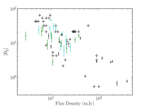
Figure 6.— Magnetic field detections and upper limits are shown relative to the flux density of the 1667 MHz line. For OHMs with detected Zeeman splitting, the flux density used is that of the Gaussian component with which the Zeeman splitting was associated. For upper limits, the plotted flux density is the peak flux density of the line. The most confident detected fields are black, moderate quality detections are green, and the marginal detections are cyan.

6.1. Comparison with Galactic OH masers

R08 compared their measured magnetic field strengths with results from OH masers in the Milky Way. Combining results from Reid & Silverstein (1990) and Fish et al. (2003), R08 noted that in Galactic OH maser Zeeman pairs, the mean was 0 mG, within the 3.3 mG error in the distribution. In a similar survey, Fish et al. (2005) detected a total of 184 Zeeman pairs among all OH lines. A companion paper presenting detailed analysis of these data (Fish & Reid, 2006) shows their distribution of magnetic field magnitudes peaked at 4 mG, and fell off quickly thereafter. The two strongest observed fields, in W51 e2, had magnitudes of 19.8 mG and 21 mG. The results from R08 were broadly similar, as the median field detected had a magnitude of $\sim$3 mG, and from that R08 concluded that when examined on small scales, star formation in (U)LIRGs proceeds similarly to star formation in the Milky Way. The results from this larger survey suggest that strong fields may be more common in OHMs than in Galactic OH masers.

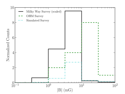
Figure 7.— Three distributions of magnetic field strengths are compared. The black solid line shows the results from the survey of Galactic OH masers by Fish et al. (2005). The dashed green line shows the distribution of magnetic fields we found in OHMs. The dash-dot cyan line represents the expected distribution we would have observed in OHMs if magnetic fields in OHMs had comparable strength to magnetic fields in Galactic OH masers.

Direct comparison of the two distributions of detected field strengths is misleading, however, as the Fish et al. (2005) magnetic field limits were far lower than the limits of this OHM survey. To better compare the two distributions, we simulated an experiment where magnetic field strengths were drawn from the observed distribution of magnetic fields observed in Galactic OH masers. This was made up of the Fish et al. (2005) distribution, plus a $\sim$40 mG field discovered in W75N (Slysh & Migenes, 2006). The limits for the simulated survey were drawn from our own results.

The sample of limits was created in the following way. For sources with detections, we counted each detected field associated with a Gaussian component, and used four times the error associated with that component as the limit, since our reported upper limits were found by taking the reported field strength and adding three times the reported error. For sources with no detection, we used the upper limit for magnetic fields in the source reported above. Then, we randomly drew a magnetic field strength from the Galactic OH maser magnetic field distribution and a limit from our distribution, and recorded fields larger than the limits as detections. For a single run, this process was repeated $n$ times, where $n$ was the number of values in the upper limit distribution.

We then simulated $10^{4}$ surveys in which the magnetic field strengths in the OHM sample were distributed according to the distribution observed in the Milky Way. The results of this simulated survey are shown in Figure 7, alongside the distribution of fields in Milky Way OH masers reported in Fish et al. (2005), and the distribution we actually observed. The three distributions are clearly distinct. If the magnetic fields in OHMs were drawn from the same distribution as those in Galactic OH masers, we would have detected many fewer fields overall, and, most notably, many fewer strong fields. Fields stronger than 10 mG are apparently much more common in OHMs than in the Milky Way.

The results of this simulated survey were consistently different than what we observed. The median of the median magnitude magnetic field detected in the simulated surveys was 5.0 mG, and 95% of the medians fell between 4.0–5.5 mG. The 12 mG median of OHM magnetic fields in the actual survey is more than a factor of two larger than the typical median in the simulated samples. Altogether, these results argue that the magnetic fields in OHMs are stronger than those in Milky Way OH masers.

6.2. Strong Fields and Time Variability

R08 reported a factor of $\sim$2 variation in one component of the emission from IRAS F12032+1707, and noted that the magnetic field associated with that component was the strongest observed in their observations. R08 noted that a connection between strong fields and time variability had been observed in Galactic OH masers, as Slysh & Migenes (2006) and Fish & Reid (2007) both reported 40 mG fields in W75N that are associated with maser spots in the process of flaring.

Our more recent observations of magnetic fields in OHMs do not provide any further evidence of this connection, though the observations do not provide strong contrary evidence either. There is weak variability, at the 1–10% level, observed in four of the six OHMs re-observed in this survey. The strongest variability observed here occurs in IRAS F12112+0305, in which the upper limit on magnetic field magnitude is $\sim$3 mG, and in III Zw 35, which has magnetic fields with magnitudes of $\sim$3 mG in the region where variability occurs. In IRAS F12032+1707, any further variability since the observations of R08 is limited. In comparing other sources with strong fields detected in our survey with existing spectra in the literature, we encounter no instances similar to IRAS F12032+1707, where a component with a strong magnetic field has clearly varied relative to its previously published strength.

6.3. Dynamical importance

The small number of OHMs with VLBI observations show reasonable diversity, with compact, parsec-scale emission providing the majority of emission in some sources (Arp 220, III Zw 35, IRAS F17208–0014), while compact emission is weak or absent in others (Mrk 231, IRAS F14070+0525), and in one case, emission was compact on the $\sim$100 pc resolution of the observations (IRAS F12032+1707). Of the strong Zeeman splitting signals observed in Arp 220 and III Zw 35, most could be associated with these compact, parsec-scale features. If all strong magnetic fields detections presented here, including those in sources without VLBI observations, occur in parsec-scale regions, it suggests that magnetic fields may be dynamically important in masing clouds in OHMs.

In the modeling of OHM emission in III Zw 35 by Parra et al. (2005), they assumed a maximum density of $n_{\rm H_{2}}=10^{5}\;{\rm cm}^{-3}$ in their OHM clouds, a cloud size of roughly $R=1$ pc, and noted that typical internal velocity dispersions are $\Delta V=20$ $\;{\rm km\;s}^{-1}$. We take these values as being reasonably representative of OHMs at large, and explore the implications of the observed magnetic field strengths. While this is surely imperfect, the small sample of VLBI measurements indicates that III Zw 35 is not unusual in its small scale properties.

Following the Stahler & Palla (2005) application of the virial theorem to a spherical cloud, and assuming its mass is dominated by molecular hydrogen, the ratio of the magnetic energy density, $\mathcal{M}$, to the self gravitational energy, $\mathcal{W}$, is

$$\frac{\mathcal{M}}{\left|\mathcal{W}\right|}\simeq 0.5\left(\frac{B}{3{\rm\;mG}}\right)^{2}\left(\frac{R}{1{\rm\;pc}}\right)^{-2}\left(\frac{n_{\rm H_{2}}^{2}}{10^{5}\;{\rm cm}^{-3}}\right)^{-2}.$$ (4)

R08 found $\sim$3 mG line-of-sight magnetic fields in III Zw 35. For a variety of plausible magnetic field probability distribution functions, the mean of the line-of-sight magnetic fields is roughly half the mean of the true magnetic field strength (Heiles & Crutcher, 2005). This suggests that the typical magnetic fields observed in OHMs are dynamically important, and perhaps even dominant.

Parra et al. (2005) note, however, that the clouds in III Zw 35 have typical velocity dispersions of $\sim$20 $\;{\rm km\;s}^{-1}$ and are not likely gravitationally confined, and then go on to suggest that magnetic fields could play a role in magnetically confining the clouds. The ratio of the magnetic energy density and the turbulent energy density, $\mathcal{T}$, are equal for

$$\frac{\mathcal{M}}{\left|\mathcal{T}\right|}\simeq 0.2\left(\frac{B}{3{\rm\;mG}}\right)^{2}\left(\frac{\Delta V}{20{\rm\;\;{\rm km\;s}^{-1}}}\right)^{-2}\left(\frac{n_{\rm H_{2}}^{2}}{10^{5}\;{\rm cm}^{-3}}\right)^{-1}.$$ (5)

This expression shows that for total magnetic field strengths a factor of two stronger than the observed line-of-sight fields, and values for the velocity dispersion and cloud size used in Parra et al. (2005), the turbulent pressure and magnetic pressure are of roughly equal strength. Altogether, these results argue that magnetic fields are important in determining the structure of OH masing clouds in at least some fraction of OHMs.

Densities in Galactic OH maser regions are of order $10^{6}$–$10^{7}\;{\rm cm}^{-3}$ (Reid et al., 1987), as measured by NH₃. If extragalactic OH megamasers mase at similar densities, the weaker ($\sim$3 mG) magnetic fields detected in this survey would not be dynamically important, unless clouds are a factor of a few smaller than 1 pc. However, for sources with $\sim$20–30 mG fields, magnetic fields would still be dynamically relevant in a $\sim$1 pc cloud, even at densities of $10^{6}\;{\rm cm}^{-3}$. More VLBI observations of OHMs with magnetic fields, particularly the strongest magnetic fields, will be necessary to developing a better understanding of the role magnetic fields play in the central regions of OHM hosts.

7. Conclusions

We performed Full-Stokes observations of seventy-seven OH megamasers, representing the entire known sample of Arecibo accessible OHMs known at the time of observations. Six of these sources had recently been observed in Full-Stokes mode by Robishaw et al. (2008), and four of those six sources had features in their Stokes $V$ spectra consistent with Zeeman splitting. We confirm the Stokes $V$ detections in three of the four sources, the non-detections in the two sources without Stokes $V$ features, and find that the apparent Zeeman splitting in one of the four sources was actually interference. Of the remaining seventy-one sources without previous Stokes $V$ observations, eleven have features consistent with Zeeman splitting in the Stokes $V$ spectra.

For all sources with Stokes $V$ features, we derived magnetic field strengths that could produce the observed Zeeman splitting signal. The median magnetic field magnitude associated with masing components in the fourteen OHMs with Zeeman detections is 12 mG. We show that the magnetic field strengths observed in OHM masing clouds are roughly a factor of 2–3 larger than those observed in Galactic OH masers. The strongest derived magnetic field in which we are confident has a magnitude of 27.6 mG. One source, IRAS F04332+0209, appears to have Zeeman splitting that exceeds the linewidth. This interpretation cannot be confirmed without VLBI observations, but if it is correct, the required magnetic field strength would be $\sim$47 mG. In two other sources, IRAS 02524+2046 and IRAS F18588+3517, we observed for the first time Zeeman splitting in the 1665 MHz OH line of an OHM. In each case, the reported magnetic field strength is consistent with that derived for the 1667 MHz line at the same velocity. For reasonable assumptions about conditions in OHMs, the magnetic field measurements presented here argue for magnetic fields playing a dynamically important role in the masing clouds.

We thank Tim Robishaw for sharing code he developed for analyzing and reducing Full-Stokes Arecibo data. We also thank Eliot Quataert and Moshe Elitzur for many helpful discussions. We thank the anonymous referee for constructive comments that improved this paper. This research was supported in part by NSF grant AST-0908572. J. M. received support from a NSF Graduate Research Fellowship. This research used NASA’s Astrophysics Data System Bibliographic Services, the SIMBAD database, operated at CDS, Strasbourg, France, and the NASA/IPAC Extragalactic Database (NED), which is operated by the Jet Propulsion Laboratory, California Institute of Technology, under contract with the National Aeronautics and Space Administration. Cosmological calculations used CosmoloPy (${\rm http://roban.github.com/CosmoloPy/}$), a cosmology package for Python.

References

- Baan et al. (1989) Baan, W. A., Haschick, A., & Henkel, C. 1989, The Astrophysical Journal, 346, 680
- Baan et al. (1992) Baan, W. A., Haschick, A. D., & Henkel, C. 1992, The Astronomical Journal, 103, 728
- Baan et al. (1987) Baan, W. A., Henkel, C., & Haschick, A. D. 1987, The Astrophysical Journal, 320, 154
- Baan et al. (1998) Baan, W. A., Salzer, J. J., & LeWinter, R. D. 1998, The Astrophysical Journal, 509, 633
- Bottinelli et al. (1989) Bottinelli, L., Gouguenheim, L., Le Squeren, A. M., Dennefeld, M., Martin, J. M., & Paturel, G. 1989, IAU Circ., 4928, 2
- Bottinelli et al. (1990) —. 1990, IAU Circ., 4977, 2
- Bottinelli et al. (1985) Bottinelli, L., Gouguenheim, L., Le Squeren, A. M., Dennefeld, M., & Paturel, G. 1985, IAU Circ.
- Bottinelli et al. (1986) Bottinelli, L., Gouguenheim, L., Le Squeren, A. M., Martin, J. M., Dennefeld, M., & Paturel, G. 1986, IAU Circ., 4231, 2
- Bottinelli et al. (1987) —. 1987, IAU Circ., 4357, 3
- Condon et al. (1991) Condon, J. J., Huang, Z.-P., Yin, Q. F., & Thuan, T. X. 1991, The Astrophysical Journal, 378, 65
- Darling (2007) Darling, J. 2007, The Astrophysical Journal, 669, L9
- Darling & Giovanelli (2000) Darling, J., & Giovanelli, R. 2000, The Astronomical Journal, 119, 3003
- Darling & Giovanelli (2001) —. 2001, The Astronomical Journal, 121, 1278
- Darling & Giovanelli (2002a) —. 2002a, The Astronomical Journal, 124, 100
- Darling & Giovanelli (2002b) —. 2002b, The Astrophysical Journal, 572, 810
- Darling & Giovanelli (2006) —. 2006, The Astronomical Journal, 132, 2596
- Diamond et al. (1999) Diamond, P. J., Lonsdale, C. J., Lonsdale, C. J., & Smith, H. E. 1999, The Astrophysical Journal, 511, 178
- Dickey et al. (1990) Dickey, J. M., Planesas, P., Mirabel, I. F., & Kazes, I. 1990, AJ, 100, 1457
- Efron & Tibshirani (1993) Efron, B., & Tibshirani, R. 1993, An introduction to the bootstrap, Monographs on statistics and applied probability (Chapman & Hall)
- Fish & Reid (2006) Fish, V. L., & Reid, M. J. 2006, The Astrophysical Journal Supplement Series, 164, 99
- Fish & Reid (2007) —. 2007, The Astrophysical Journal, 656, 952
- Fish et al. (2003) Fish, V. L., Reid, M. J., Argon, A. L., & Menten, K. M. 2003, The Astrophysical Journal, 596, 328
- Fish et al. (2005) Fish, V. L., Reid, M. J., Argon, A. L., & Zheng, X. 2005, The Astrophysical Journal Supplement Series, 160, 220
- Garwood et al. (1987) Garwood, R., Dickey, J., & Helou, G. 1987, The Astrophysical Journal, 322, 88
- Heiles & Crutcher (2005) Heiles, C., & Crutcher, R. 2005, Cosmic Magnetic Fields, 182, 137
- Heiles et al. (1993) Heiles, C., Goodman, A. A., McKee, C. F., & Zweibel, E. G. 1993, In: Protostars and planets III (A93-42937 17-90), 279
- Hinshaw et al. (2009) Hinshaw, G., et al. 2009, ApJS, 180, 225
- Kandalian et al. (2007) Kandalian, R. A., Hambaryan, V. V., & Sabat, H. a. 2007, Astrophysics, 50, 135
- Kazes & Baan (1991) Kazes, I., & Baan, W. A. 1991, Astronomy and Astrophysics (ISSN 0004-6361), 248
- Lawrence et al. (1999) Lawrence, A., et al. 1999, MNRAS, 308, 897
- Lo (2005) Lo, K. 2005, Annual Review of Astronomy and Astrophysics, 43, 625
- Lockett & Elitzur (2008) Lockett, P., & Elitzur, M. 2008, The Astrophysical Journal, 677, 985
- Lonsdale & Smith (2003) Lonsdale, C., & Smith, H. 2003, The Astrophysical, 592, 804
- Lonsdale et al. (2008) Lonsdale, C. J., de Kleer, K. R., Diamond, P. J., Thrall, H., Lonsdale, C. J., & Smith, H. E. 2008, Proceedings of the International Astronomical Union, 3, 432
- Lonsdale et al. (1998) Lonsdale, C. J., Lonsdale, C. J., & Diamond, P. J. 1998, The Astrophysical Journal, 493, 13
- Martin et al. (1989) Martin, J., Bottinelli, L., Gouguenheim, L., Le Squeren, A., & Dennefeld, M. 1989, Academie des Sciences Paris Comptes Rendus Serie Sciences Mathematiques, 308, 287
- Martin et al. (1988a) Martin, J. M., Bottinelli, L., Dennefeld, M., Gouguenheim, L., Handa, T., Le Squeren, A. M., Nakai, N., & Sofue, Y. 1988a, Astronomy and Astrophysics, 195, 71
- Martin et al. (1988b) Martin, J. M., Le Squeren, A. M., Bottinelli, L., Gouguenheim, L., & Dennefeld, M. 1988b, Astronomy and Astrophysics (ISSN 0004-6361), 201
- Martin et al. (1989) —. 1989, Astronomy and Astrophysics (ISSN 0004-6361), 208, 39
- Martin et al. (1989) Martin, J. M., Le Squeren, A. M., Bottinelli, L., Gouguenheim, L., & Dennefeld, M. 1989, A&A, 208, 39
- Mirabel & Sanders (1987) Mirabel, I. F., & Sanders, D. B. 1987, The Astrophysical Journal, 322, 688
- Momjian et al. (2006) Momjian, E., Romney, J. D., Carilli, C. L., & Troland, T. H. 2006, The Astrophysical Journal, 653, 1172
- Parra et al. (2005) Parra, R., Conway, J. E., Elitzur, M., & Pihlström, Y. M. 2005, Astronomy and Astrophysics, 443, 383
- Pihlström et al. (2001) Pihlström, Y., Conway, J., Booth, R., Diamond, P., & Polatidis, A. 2001, Astronomy and Astrophysics, 377, 413
- Pihlström et al. (2005) Pihlström, Y. M., Baan, W. A., Darling, J., & Klöckner, H. 2005, The Astrophysical Journal, 618, 705
- Reid et al. (1987) Reid, M. J., Myers, P. C., & Bieging, J. H. 1987, The Astrophysical Journal, 312, 830
- Reid & Silverstein (1990) Reid, M. J., & Silverstein, E. M. 1990, The Astrophysical Journal, 361, 483
- Robishaw et al. (2008) Robishaw, T., Quataert, E., & Heiles, C. 2008, The Astrophysical Journal, 680, 981
- Schmelz et al. (1986) Schmelz, J., Baan, W. A., Haschick, A. D., & Eder, J. 1986, The Astronomical Journal, 92, 1291
- Slysh & Migenes (2006) Slysh, V. I., & Migenes, V. 2006, Monthly Notices of the Royal Astronomical Society, 369, 1497
- Stahler & Palla (2005) Stahler, S. W., & Palla, F. 2005, The Formation of Stars
- Stanford et al. (2000) Stanford, S. A., Stern, D., van Breugel, W., & De Breuck, C. 2000, The Astrophysical Journal Supplement Series, 131, 185
- Thompson et al. (2006) Thompson, T. a., Quataert, E., Waxman, E., Murray, N., & Martin, C. L. 2006, The Astrophysical Journal, 645, 186
- Troland & Heiles (1982) Troland, T. H., & Heiles, C. 1982, The Zeeman effect in 21 centimeter line radiation: Methods and initial results
- Vignali et al. (2005) Vignali, C., Brandt, W. N., Comastri, A., & Darling, J. 2005, Monthly Notices of the Royal Astronomical Society, 364, 99
- Willett et al. (2011a) Willett, K., Darling, J., Spoon, H. W. W., Charmandaris, V., & Armus, L. 2011a, The Astrophysical Journal Supplement Series, 193, 18
- Willett et al. (2011b) —. 2011b, The Astrophysical Journal, 730, 56
- Willett (2012) Willett, K. W. 2012, Cosmic Masers from OH to H_O, 119