Undulations from amplified low frequency surface waves

Abstract

We study the linear scattering of gravity waves in longitudinal inhomogeneous stationary flows. When the flow becomes supercritical, it is known that counterflow propagating shallow waves are blocked and converted into deep waves. Here we show that in the zero-frequency limit, the reflected waves are amplified in such a way that the free surface develops an undulation, i.e., a zero-frequency wave of large amplitude with nodes located at specific places. This amplification involves negative energy waves, and implies that flat surfaces are unstable against incoming perturbations of arbitrary small amplitude. The relation between this instability and black hole radiation (the Hawking effect) is established.

I Introduction

It has long been observed that stationary flows that become supercritical, i.e., when the flow velocity equals the speed of low frequency surface waves, are often associated with an undulation, i.e., a zero-frequency wave with a macroscopic amplitude Johnson ; Lawrence87 . Undulations have been extensively studied, often in the forced and in the nonlinear regime, see e.g. Wu87 ; LeePhD ; Byatt71 ; El05 ; El05b . In this paper, we study their appearance in another regime, namely from the scattering of low frequency shallow waves which propagate against a background flow with a flat surface, i.e. when the forcing vanishes. In this case, we shall show that an undulation develops because the background flow is unstable against incoming waves with arbitrary small amplitudes. In this we have been inspired by the fact that their scattering near the blocking point is akin to that governing the Hawking effect Hawking75 ; Unruh76 ; Unruh81 ; Unruh95 ; Schutzhold02 ; Balbinot06 , which predicts that black holes should spontaneously emit a thermal flux.

To understand the scattering of counterflow waves, one must take into account their dispersion relation. In homogeneous stationary flows, when neglecting capillary effects Johnson , the relation between $\Omega$ (the frequency measured in the fluid frame) and the wave vector $k$ is given by

$$\Omega^{2}=gk\tanh(h_{B}k),$$ (1)

where $h_{B}$ is the height of the background flow, and $g$ the gravitational acceleration. When the flow is inhomogeneous, at fixed frequency $\omega$ measured in the lab frame, the co-moving frequency $\Omega$ becomes a function of $x$ given by $\omega=\Omega+v_{x}(x)k_{\omega}$, where $v_{x}(x)$ is the longitudinal velocity flow, and $k_{\omega}$ the $x$-dependent wave vector. When $\omega$ is high enough, a counter flow wave packet is blocked and generates two reflected wave packets, a long wavelength co-propagating mode, and a short wavelength one which is dragged by the flow. In this case, the (positive) incoming energy is shared among the two outgoing waves. When lowering $\omega$ below of certain critical frequency $\omega_{\kappa}$, which is related to the gradient of $v_{x}(x)$ evaluated when $F_{n}$ crosses 1, a third wave acquires a non-negligible amplitude. (We define the Froude number $F_{n}$ as the ratio of the flow velocity $v_{x}$ over the speed of low frequency waves.) This extra wave possesses a negative energy, which means that we are now facing an over-reflection Acheson76 , i.e., an amplification process. In a recent experiment Weinfurtner10 ; Weinfurtner13 , the production of this extra wave have been clearly observed in the linear regime we shall use.

In the present paper, we study a limit which was not studied in Unruh81 ; Schutzhold02 ; Rousseaux07 ; Weinfurtner10 ; Unruh12 . It concerns the limit $\omega\ll\omega_{\kappa}$. In this case, the long wavelength co-propagating mode plays no significant role, while unusual properties characterize the two short wavelength modes of opposite energy. First, in the limit $\omega\to 0$, they acquire the same amplitude, merge, and form a single standing wave with zero frequency and nodes at definite places. Second, the amplification factor diverges as $1/\omega$. Using the correspondence with black hole geometry, we show that this divergence is directly related to the famous prediction of Hawking radiation Hawking75 . Using the fact that perturbations of inhomogeneous flows propagate as light waves on a curved space-time Unruh81 , one realizes that the supercritical flows we consider correspond to “acoustic white holes” Schutzhold02 ; Rousseaux07 ; Weinfurtner10 ; Unruh12 with their horizon located where $F_{n}=1$. In fact, the generation of undulations and black hole emission are based on a common amplification mechanism. This explains why undulations have been observed in the experiments Rousseaux07 ; Weinfurtner10 ; Weinfurtner13 aiming at measuring the analogue Hawking effect.

The paper is organized as follows. In Section II, we present the wave equation, discuss the scattering of stationary waves in supercritical flows, and demonstrate that the amplification factor diverges as $1/\omega$ for $\omega\to 0$. In Section III, we study incoming waves packets and show that the two reflected waves merge and form a single undulation in the limit $\omega\to 0$. We then show that incident low frequency waves with random properties also give rise to the same undulation, but with a growing amplitude. In Appendix A, we derive the wave equation and relate it to the relativistic equation used by Hawking. In Appendix B, we review the main properties of the conserved inner product which governs the amplification process. In Appendix C, we explain how to compute the amplification factor without having recourse to standard WKB techniques which fail in the present case.

II Settings

In this Section, we adapt to the present case results which have been recently obtained in other works. The important new results are presented in the next Section.

II.1 Wave equation et action formalism

We consider surface waves which propagate in a water tank of constant transverse dimension $L_{\perp}$. We assume that the flow is incompressible, non turbulent, and irrotational. We also assume that both the bottom of the tank and the background free surface do not depend on the transverse coordinate, and become asymptotically flat in the upstream region. We call $h_{\rm as}$ and $v_{\rm as}$ the asymptotic values of the water depth and the background flow velocity in this region. For simplicity, we only study waves with no dependence in the transverse coordinate, and we neglect the effects of capillarity. To incorporate the latter, one should consider the dispersion relation which generalizes Eq. (1) by including the capillary length Schutzhold02 . Including these short wavelength effects will not affect the main conclusions of our work.

When the background flow is non-uniform, the linear equation for surface waves is rather complicated Schutzhold02 ; Unruh12 . The origin of the difficulty stems from the fact that we aim to study the zero frequency limit. As a result, we cannot use the standard slowly varying (WKB) approximation where the wave vector $k_{\omega}$ is much larger than the typical spatial gradient of the background flow. In Appendix A, we recall the main steps to obtain it and compare it with other models of water waves. In the body of the text, we shall exploit the fact that this equation can be derived from an action. Interestingly, this action possesses a rather simple structure which, moreover, is very similar to that describing sound waves in an irrotational fluid Balbinot06 . In addition, the action formalism is appropriate to efficiently describe the wave scattering, as well as to establish the relationship with the Hawking treatment of black hole radiation.

The action for the perturbations $\phi$ of the velocity potential has the following structure

$$S=\frac{1}{2}\int\rho(x)\left\{\frac{1}{c^{2}(x)}[(\partial_{t}+v_{x}(x)\,\partial_{x})\phi]^{2}-\phi\,\hat{F}^{2}(d_{\Lambda}(x))\,\phi\right\}dxdt.$$ (2)

The function $\rho(x)$ is an effective 1-dimensional fluid density, $v_{x}(x)$ is the background flow velocity, $c(x)$ fixes the low frequency group velocity, and $\hat{F}^{2}$ is a differential operator which governs the dispersion relation. The combination $\rho\hat{F}^{2}$ forms a self-adjoint operator, and $d_{\Lambda}(x)$ is the local dispersive wavelength. (In an atomic Bose condensate, the latter is known as the healing length Dalfovo99 ; Macher09b .) For each fluid, these functions are related in a specific manner to the properties of the background flow.

For gravity waves, assuming an incompressible fluid, i.e., a constant 3-dimensional density $\rho_{0}^{3D}$, there are several (physically equivalent) ways to identify these functions. Using the results of Appendix A, a convenient choice is

$$\hat{F}^{2}(d_{\Lambda}(x)) = \frac{1}{d_{\Lambda}(x)}i\partial_{x}\tanh(d_{\Lambda}(x)i\partial_{x}),$$ (3a)

$$d_{\Lambda}(x) = h_{\rm as}\frac{v_{\rm as}v_{x}(x)}{v^{2}(x)},$$ (3b)

$$\rho(x) = \rho_{0}^{3D}L_{\perp}d_{\Lambda}(x),$$ (3c)

$$c^{2}(x) = d_{\Lambda}(x)\left[g+\frac{v_{x}^{2}}{v^{2}}\partial_{y}(v^{2}/2)_{y\,=\,h_{B}(x)}\right]\doteq d_{\Lambda}(x)\,g_{\rm eff}(x).$$ (3d)

In the above, $v^{2}=v_{x}^{2}+v_{y}^{2}$, where $v_{x}$ and $v_{y}$ are the horizontal and vertical components of the background velocity, evaluated along the free surface $y=h_{B}(x)$. (Note that the local Froude number is now unambiguously defined as $F_{n}=v_{x}(x)/c(x)$.) The quantity $g_{\rm eff}$ is the effective gravitational acceleration which takes into account the centrifugal acceleration. Asymptotically, all $x$ dependence are negligible, and Eq. (3d) delivers the standard expression $c_{\rm as}^{2}=h_{\rm as}g$. For long wavelengths, i.e. low gradients $kd_{\Lambda}\ll 1$, the dispersive length $d_{\Lambda}$ drops out from Eq. (3a) and one gets the dispersionless expression $F^{2}\to k^{2}$, since $k=-i\partial_{x}$. For smaller wavelengths, combining $F^{2}$ and $c^{2}$, one finds a generalized version of Eq. (1) where $d_{\Lambda}$ acts as a dressed value of $h_{\rm as}$. In fact, to lowest order in $\partial_{y}v_{x}$, one can show that $d_{\Lambda}(x)$ reduces to the water depth at $x$ (see Eq. (72) in Appendix A).

As far as the scattering of waves is concerned, all we need is the knowledge of the differential operator $\hat{F}^{2}$ and the functions $\rho,v,c,d_{\Lambda}$ entering in Eq. (2). In other words, the intricate aspects of the above equations will play no significant role in the sequel. Yet, to make physical predictions, and to test them, one needs the relation between the velocity potential $\phi$ and the vertical fluctuation of the surface $\delta h(t,x)=h(t,x)-h_{B}(x)$ with respect to the background free surface $y=h_{B}(x)$. As explained in Appendix A, see (74), this relation is

$$\delta h(t,x)=-\frac{1}{g_{\rm eff}(x)}(\partial_{t}+v_{x}(x)\partial_{x})\phi(t,x).$$ (4)

It is interesting to notice that $\delta h(t,x)$ is related by a constant factor to $\pi(t,x)$, the momentum conjugated to $\phi(t,x)$ given the action of Eq. (2) . Indeed, taking the variation of the action with respect to $\partial_{t}\phi$, one obtains

$$\pi(t,x) \doteq \frac{\rho(x)}{c^{2}(x)}(\partial_{t}+v_{x}(x)\partial_{x})\phi(t,x),$$ (5a)

$$= -(\rho_{0}^{3D}L_{\perp})\,\delta h(t,x).$$ (5b)

It is also interesting to notice that for sound waves, e.g. in an atomic Bose condensate, the density fluctuation $\delta\rho$ is related to the momentum $\pi$, and the potential $\phi$, by very similar equations, see Eq. (B.11) in Macher09b . Therefore the forthcoming analysis also applies to these waves, when using the appropriate $\hat{F}^{2}$ operator governing dispersion.

When applying the Legendre transform ($H\doteq\pi\partial_{t}\phi-\mathcal{L}$) to the action density of Eq. (2), one obtains the Hamiltonian

$$H=\frac{1}{2}\int\frac{\rho}{c^{2}}\left\{\left[\frac{c^{2}\pi}{\rho}-v_{x}\,\partial_{x}\phi\right]^{2}-v_{x}^{2}(\partial_{x}\phi)^{2}+c^{2}\,\phi\hat{F}^{2}(d_{\Lambda})\phi\right\}dx.$$ (6)

For stationary flows, $H$ is conserved and furnishes the energy carried by the waves. For homogeneous backgrounds, Eq. (6) coincides with standard expression Dingemans . The wave equation can then be obtained from Hamilton equations. The first equation $\partial_{t}\phi=\{\phi,H\}$, where $\{\,,\}$ is the Poisson bracket, gives back Eq. (5a). The second equation, $\partial_{t}\pi=\{\pi,H\}$, gives

$$(\partial_{t}+\partial_{x}v_{x}(x))\pi(t,x)=-\rho(x)\hat{F}^{2}(d_{\Lambda}(x))\,\phi(t,x),$$ (7)

which corresponds to Eq. (86) in Unruh12 . Taken together, these equations give

$$\left[(\partial_{t}+\partial_{x}v_{x}(x))\frac{\rho(x)}{c^{2}(x)}(\partial_{t}+v_{x}(x)\partial_{x})+\rho(x)\hat{F}^{2}(d_{\Lambda}(x))\right]\phi(t,x)=0.$$ (8)

The forthcoming analysis is based on this wave equation applied to supercritical flows as that depicted on Fig.1. We emphasize that we shall neither make use of the standard slowly varying approximation, i.e., $\kappa/c_{0}\ll k_{\omega}$ in term of the typical frequency defined in the Figure caption, nor assume that the flow is near critical, (i.e., $|F_{n}-1|\ll 1$). Our treatment thus applies to arbitrary low frequencies, and is valid in flows where $v$ and $c$ significantly vary. This contrasts with the regimes commonly explored, e.g. in Johnson ; Mei ; Dingemans (for further discussion on this, see App. A.4).

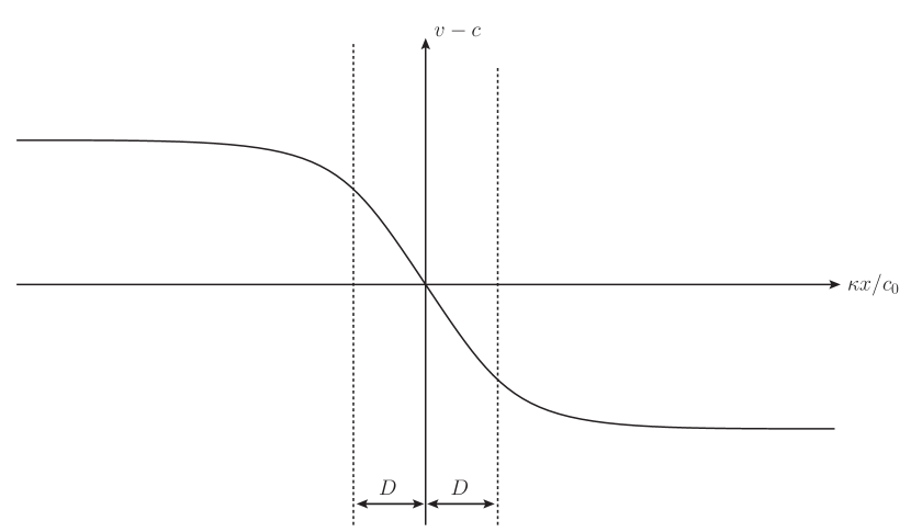
Figure 1: Background profile $v_{x}-c$ as a function of $x$ with $v>0$. The chosen profile is $v_{x}-c=-c_{0}D\tanh\left({\kappa x}/{c_{0}D}\right)$, where $c_{0}$ is the speed at $x=0$. The parameter $D$ governs the extension of the near wave blocking region where $c-v_{x}\sim\kappa x$. The frequency $\kappa$ is defined by $\partial_{x}(v_{x}-c)_{|x=0}=-\kappa$. As explained in App. C it governs both the spatial properties of the modes in this region, and the non-trivial mode mixing. In a gravitational context, it is known as the surface gravity Unruh81 . On the asymptotic subcritical right side, $v_{x}(x)$ and $c(x)$ reach the constant values $v_{\rm as}$ and $c_{\rm as}$.

II.2 Incoming and outgoing mode bases

To study the scattering of monochromatic waves of fixed frequency $\omega$, we introduce the complex modes $e^{-i\omega t}\phi_{\omega}(x)$. Eq. (8) implies that their spatial part obeys

$$\left[(\omega+i\partial_{x}v_{x}(x))\frac{\rho(x)}{c^{2}(x)}(\omega+iv_{x}(x)\partial_{x})-\rho(x)\hat{F}^{2}(d_{\Lambda}(x))\right]\phi_{\omega}(x)=0.$$ (9)

The real time-dependent wave is then given by $\phi(t,x)=2\textrm{Re}\left(e^{-i\omega t}\phi_{\omega}(x)\right)$. To describe the scattering, we use two different mode bases, for more details in a similar context see Macher09 . The in basis describes modes that shall be scattered, while the out one describes modes that have been scattered. These modes are identified through the standard procedure Greiner ; Fulling ; Primer : in the past (resp. in the future), each incoming mode $\phi_{\omega}^{\rm in}$ (resp. outgoing $\phi_{\omega}^{\rm out}$) asymptotes in the sense of a broad wave packet to a single plane wave with a group velocity $v_{g}=(\partial_{\omega}k)^{-1}$ directed toward (resp. away from) the blocking point. These asymptotic plane waves are given by $\sim e^{ik_{\omega}^{a}x}$ where $k^{a}_{\omega}$ is a real root of the dispersion relation

$$(\omega-v_{\rm as}k^{a}_{\omega})^{2}=gk^{a}_{\omega}\tanh\left(h_{\rm as}k^{a}_{\omega}\right)=(\Omega^{a}_{\omega})^{2}.$$ (10)

As a result, the number of independent modes is equal to the number of real solutions of Eq. (10) with $\omega>0$.

For this reason, it is worth studying these roots. On the right asymptotic side, where the flow is subcritical ($|v_{\rm as}|<c_{\rm as}$), there is a threshold value $\omega_{\rm max}$ which separates two cases. For $\omega$ above $\omega_{\rm max}$, there are 2 real roots, as in the absence of a flow. Instead, in the low frequency regime which interests us, for $0<\omega<\omega_{\rm max}$, there are 4 real roots, see Fig. 2, which means that there two new types of stationary waves. Because each asymptotic root corresponds to either an in or out mode, we call the various roots using the name of the corresponding mode. For instance, $k_{\omega}^{\rm in}$ describes the (usual) long wavelength incoming left moving mode $\phi_{\omega}^{\rm in}$. When $\omega\to 0^{+}$, one has

$$k_{\omega}^{\rm in}\sim-\frac{\omega}{c_{\rm as}-v_{\rm as}}=\omega/v_{g}^{\rm in}<0.$$ (11)

The group velocity $v_{g}^{\rm in}=-c_{\rm as}+v_{\rm as}<0$ confirms that it is moving leftward. The positive long wavelength root $k_{\omega}^{\rm co,\,out}$ describes the (usual) co-moving outgoing mode $\phi_{\omega}^{\rm co,\,out}$ since $v_{g}^{{\rm co,\,out}}=c_{\rm as}+v_{\rm as}>0$. The last roots $k_{\omega}^{\rm out}<0$ and $-k_{-\omega}^{\rm out}>0$ are the two new ones. They both correspond to short wavelengths conter-propagating modes which are both swept along with the flow. When $\omega\to 0$, as clearly seen in Fig. 2, they reach opposite value $\mp k_{Z}$ respectively, with $k_{Z}>0$. More precisely, to first order in $\omega$

$$k_{\omega}^{\rm out}=-k_{Z}+\omega/v_{g}^{Z},$$ (12)

where $v_{g}^{Z}>0$.

In Fig. 2, one also notices that three of the four roots, namely $k_{\omega}^{\rm in}$, $k_{\omega}^{\rm co,\,out}$ and $k_{\omega}^{\rm out}$, live on the branch of solutions with a positive comoving frequency $\Omega_{\omega}=\omega-v_{\rm as}k_{\omega}$. This branch characterizes the modes with positive energy and positive norm, see App.B for more details concerning this important aspect. Instead, the fourth root has a negative energy, and lives in the “unusual” branch of solutions of negative $\Omega$ and negative norm. To keep this in mind, we call this root $-k_{-\omega}^{\rm out}$. First, because $k_{-\omega}^{\rm out}<0$ lives on the usual branch when considering the opposite value of $\omega$, and second, because the curves of Fig. 2 are left invariant under both $\omega\to-\omega$ and $k\to-k$, which replaces the positive $\Omega$ branch by the negative one, and vice versa. The outgoing modes which correspond to $k_{\omega}^{\rm out}$ and $-k_{-\omega}^{\rm out}$ shall be respectively called $\phi_{\omega}^{\rm out}$ for the positive norm one, and $\left(\phi_{-\omega}^{\rm out}\right)^{*}$ for the negative norm one.

In usual circumstances, i.e. when $\omega$ is not too small, the mixing of $\left(\phi_{-\omega}^{\rm out}\right)^{*}$ with the positive norm modes is so small that it can be safely ignored. In this case, one deals with an elastic scattering. However, at low frequencies, for supercritical flows like that of Fig. 1, the mixing becomes so important that it is must be included to account for the observed phenomena Rousseaux07 ; Weinfurtner10 ; Weinfurtner13 . On the other hand, the co-propagating mode $\phi_{\omega}^{\rm co}$ plays essentially no role . Hence, we are effectively facing an “over-reflection” involving only two pairs of modes.

The two out modes $\phi_{\omega}^{\rm out},(\phi_{-\omega}^{\rm out})^{*}$, and the in mode $\phi_{\omega}^{\rm in}$ have been already described. The last one is the negative norm mode $(\phi_{-\omega}^{\rm in})^{*}$. At early times, it asymptotically describes an incoming mode which comes from the left super-critical region. The corresponding root is negative and called $-k_{-\omega}^{\rm in}$ because it has a negative $\Omega$, and carries a negative energy.

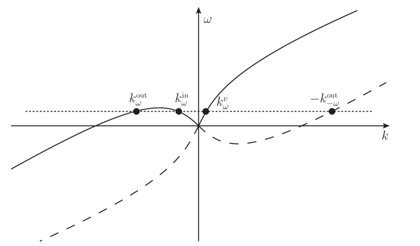
Figure 2: Dispersion relation of Eq. (10) in the $\omega-k$ plane when $v_{\rm as}>0$ and sub-critical $v_{\rm as}<c_{\rm as}$. There are two double branches: that with $\Omega>0$ (continuous lines) characterizes the positive norm modes, see App. B, while the dashed lines describe the negative norm modes. For a low frequency $\omega>0$, there are four roots. One sees that only $-k_{-\omega}^{\rm out}>0$ lives on the second branch. As explained in the text, the corresponding mode $(\phi_{-\omega}^{\rm out})^{*}$ carries negative energy, and its mixing with the other modes leads to an over-reflection. One also sees that in the limit $\omega\to 0$, $-k_{-\omega}^{\rm out}$ and $k_{\omega}^{\rm out}$ reach $\pm k_{Z}$ respectively. As shall be shown, $k_{Z}$ is the wave vector of the undulation.

II.3 Low frequency mode amplification

Since the in modes, and the out modes, form two basis of solutions of Eq. (9) (when neglecting the co-propagating mode), they are related by a linear transformation,

$$\begin{pmatrix}\phi_{\omega}^{\rm in}\\ (\phi_{-\omega}^{\rm in})^{*}\end{pmatrix}=\begin{pmatrix}\alpha_{\omega}&\beta_{\omega}\\ \tilde{\beta}_{\omega}&\tilde{\alpha}_{\omega}\end{pmatrix}\cdot\begin{pmatrix}\phi_{\omega}^{\rm out}\\ (\phi_{-\omega}^{\rm out})^{*}\end{pmatrix}.$$ (13)

Because the modes have opposite norm, the coefficients obey the anomalous scattering relation

$$|\alpha_{\omega}|^{2}-|\beta_{\omega}|^{2}=|\tilde{\alpha}_{\omega}|^{2}-|\tilde{\beta}_{\omega}|^{2}=1,$$ (14)

in the place of the standard relation $|R_{\omega}|^{2}+|T_{\omega}|^{2}=1$ between the reflection and transmission coefficients $R_{\omega}$ and $T_{\omega}$. Eq. (14) implies that $|\alpha_{\omega}|>1$, which means that the scattering leads to an amplification of the waves.

The real task is to compute the coefficients $\alpha_{\omega}$ and $\beta_{\omega}$. It turns out that for low frequencies a proper evaluation in background profiles as in Fig. 1 is non trivial. Indeed, the standard WKB treatment gives $\beta_{\omega}\equiv 0$, which means that modes of opposite norm (and energy) do not mix. To obtain $\beta_{\omega}$ one should therefore use more involved technics. These are presented in Appendix C. The main result is as follows. When the supercritical flow is smooth enough,

$$\frac{|\beta_{\omega}|^{2}}{|\alpha_{\omega}|^{2}}=e^{-\frac{2\pi\omega}{\kappa}},$$ (15)

where $\kappa$ is the background flow frequency defined in the caption of Fig. 1. It is worth mentioning that Eq. (15) was found by Hawking Hawking75 in a gravitational context when he established that incipient black holes should emit a thermal spectrum at a temperature given by $k_{B}T_{H}=\hbar\kappa/2\pi$. A careful comparison Unruh95 ; Brout95 ; Coutant11 confirms the close connection between the scattering of waves on a supercritical flow and in a black hole geometry. The main difficulty is to properly include dispersive effects. In Appendix C, following Coutant11 , we recall that, to leading order in $\kappa d_{\Lambda}/c_{0}\ll 1$, the replacement of the dispersion relation from the relativistic one used by Hawking to that of Eq. (1) does not affect Eq. (15).

For frequencies larger than $\kappa$, Eq. (15) implies that the negative energy mode has an amplitude exponentially reduced with respect to that of the standard wave, something which has been recently verified Weinfurtner10 ; Weinfurtner13 . This is the standard adiabatic regime where modes of opposite norms do not significantly mix. Instead, in the opposite limit $\omega\to 0$, Eqs. (14), (15) imply that the coefficients diverge as

$$|\alpha_{\omega}|^{2}\sim|\beta_{\omega}|^{2}\sim\frac{\kappa}{2\pi\omega}\underset{\omega\ll\kappa}{\gg}1.$$ (16)

We here underline that this divergence is still found when the mixing with the co-propagating mode is not negligible and taken into account, and also when the inequality $\kappa d_{\Lambda}/c_{0}\ll 1$ used in Appendix C is no longer satisfied. In these cases, $\kappa$ is replaced by a frequency $\bar{\kappa}$ which depends on several quantities, see the numerical and analytical work of Finazzi12 . To indicate that our forthcoming analysis covers these cases as well, we shall use the symbol $\bar{\kappa}$.

III Scattering of low frequency wave packets

We combine the various elements of the former Section to show that flat free surfaces are unstable against incoming low frequency waves of arbitrary small amplitude. As a result, an undulation develops.

III.1 Incoming waves

Using stationary in modes, the general time-dependent solution of Eq. (8) can be written as

$$\bar{\phi}(t,x)=2\textrm{Re}\left\{\int_{0}^{\omega_{\rm max}}e^{-i\omega t}\left[a_{\omega}\,\phi_{\omega}^{\rm in}(x)+b_{\omega}\,(\phi_{-\omega}^{\rm in}(x))^{*}\right]d\omega\right\},$$ (17)

where the coefficients $a_{\omega}$ and $b_{\omega}$ weigh the contribution of $\phi_{\omega}^{\rm in}$ and $(\phi_{-\omega}^{\rm in}(x))^{*}$. We now consider a series of incoming wave packets of positive energy, sent from the right side against the flow. This means that $b_{\omega}=0$. To get explicit expressions, we work with

$$a_{\omega}=\frac{A}{n_{\bar{\omega}}^{1/2}}\exp\left({-\frac{(\omega-\bar{\omega})^{2}}{2\sigma_{0}^{2}\bar{\omega}^{2}}}\right),$$ (18)

where $A$ is a complex dimensionless amplitude $A=|A|e^{i\delta}$, and where the packets are normalized by

$$\int_{0}^{\omega_{\rm max}}|a_{\omega}|^{2}d\omega=|A|^{2}.$$ (19)

We also assume that the waves are almost monochromatic. Irrespectively of the value of $\bar{\omega}$, this is realized if

$$\sigma_{0}\ll 1.$$ (20)

In this regime, one finds $n_{\bar{\omega}}=\sigma_{0}\bar{\omega}\pi^{1/2}$. The real character of Eq. (18) guarantees that the packets are centered around $x=0$ at $t=0$.

Using the asymptotic behavior of $\phi_{\omega}^{\rm in}$ given in Eq. (80) we get

$$\bar{\phi}(x,t\to-\infty)=2\textrm{Re}\left\{\bar{N}A\int_{0}^{\infty}e^{-\frac{(\omega-\bar{\omega})^{2}}{2\sigma_{0}^{2}\bar{\omega}^{2}}}\frac{e^{-i(\omega t-k_{\omega}^{\rm in}x)}}{\sqrt{4\pi\omega c_{\rm as}}}\frac{d\omega}{n_{\sigma}^{1/2}}\right\}.$$ (21)

In the broad wave regime of Eq. (20), we can accurately evaluate the integral with a saddle point approximation. Then, using Eq. (4) asymptotically, where $g_{\rm eff}=g$, the corresponding incoming height variation is

$$\delta\bar{h}^{\rm in}(x)\sim\delta\bar{h}^{\rm in}_{A}\times\sin\left(\bar{\omega}t-k_{\bar{\omega}}^{\rm in}x+\delta\right)e^{-\frac{\sigma_{0}^{2}\bar{\omega}^{2}}{2}(t-x/v_{g}^{\rm in})^{2}},$$ (22)

where the amplitude is

$$\delta\bar{h}^{\rm in}_{A}=|A|\bar{N}\frac{\bar{\omega}h_{\rm as}}{c_{\rm as}-v_{\rm as}}\sqrt{\frac{2\sigma_{0}}{\pi^{1/2}c_{\rm as}^{3}}}.$$ (23)

As expected, the incoming wave (22) oscillates at a frequency $\bar{\omega}$, has a wavenumber $k_{\bar{\omega}}^{\rm in}$, and its envelope is propagating toward the wave blocking region at a speed $v_{g}^{\rm in}<0$. We see that the argument of $A$, the phase $\delta$, governs the precise initial positions of the nodes. We also see that at fixed $A$, its amplitude $\delta\bar{h}^{\rm in}$ decreases linearly for with $\bar{\omega}$. In this respect, it is also instructive to evaluate the conserved energy transported by the wave packet. Using Eq. (6) with Eq. (21), one finds

$$\bar{E}=2\bar{\omega}N|A|^{2}.$$ (24)

At fixed $A$, the wave energy linearly vanishes in the limit $\bar{\omega}\to 0$.

III.2 Outgoing waves

At a time near $t=0$, the packet of Eq. (21) reaches the wave blocking region around $x=0$, where it undergoes a nontrivial scattering which is governed by Eq. (13). Then two outgoing wave packets are generated and propagate to the right, see Fig 3. To analyze them, it is convenient to introduce the complex wave $\bar{\phi}_{\mathbb{C}}$, such that $\bar{\phi}=2\textrm{Re}(\bar{\phi}_{\mathbb{C}})$ in Eq. (17). At late time, using the out mode basis and Eq. (13), one finds

$$\bar{\phi}_{\mathbb{C}}(x,t\to+\infty)=\bar{\phi}_{\mathbb{C}}^{+}(t,x)+\bar{\phi}_{\mathbb{C}}^{-}(t,x).$$ (25)

The two complex waves are

$$\bar{\phi}_{\mathbb{C}}^{+}(x,t\to+\infty) = \bar{N}A\int\alpha_{\omega}e^{-\frac{(\omega-\bar{\omega})^{2}}{2\sigma_{0}^{2}\bar{\omega}^{2}}}\frac{e^{-i(\omega t-k_{\omega}x)}}{\sqrt{4\pi|\Omega_{\rm out}v_{g}^{\rm out}|}}\frac{d\omega}{n_{\sigma}^{1/2}},$$ (26a)

$$\bar{\phi}_{\mathbb{C}}^{-}(x,t\to+\infty) = \bar{N}A\int\beta_{\omega}e^{-\frac{(\omega-\bar{\omega})^{2}}{2\sigma_{0}^{2}\bar{\omega}^{2}}}\frac{e^{-i(\omega t+k_{-\omega}x)}}{\sqrt{4\pi|\Omega_{\rm out}v_{g}^{\rm out}|}}\frac{d\omega}{n_{\sigma}^{1/2}}.$$ (26b)

where $\Omega_{\rm out}=\Omega(k_{\omega}^{\rm out})$ is the co-moving frequency of the outgoing modes, and $v_{g}^{\rm out}$ their group velocity. Evaluated through a saddle point method, one obtains

$$\bar{\phi}_{\mathbb{C}}^{+}(x,t\to+\infty) \sim A_{\bar{\omega}}\times\alpha_{\bar{\omega}}\,\varphi_{\bar{\omega}}^{\rm out}(x)e^{-i\bar{\omega}t}\times e^{-\frac{\sigma_{0}^{2}\bar{\omega}^{2}}{2}(t-x/v_{g}^{\rm out})^{2}},$$ (27a)

$$\bar{\phi}_{\mathbb{C}}^{-}(x,t\to+\infty) \sim A_{\bar{\omega}}\times\beta_{\bar{\omega}}\,(\varphi_{-\bar{\omega}}^{\rm out}(x))^{*}e^{-i\bar{\omega}t}\times e^{-\frac{\sigma_{0}^{2}\bar{\omega}^{2}}{2}(t-x/v_{g}^{\rm out})^{2}},$$ (27b)

where their common amplitude factor $A_{\bar{\omega}}$ is given by

$$A_{\bar{\omega}}=A\sqrt{2\sigma_{0}\bar{\omega}\pi^{1/2}}.$$ (28)

We now have all the ingredients to consider the limit $\bar{\omega}\to 0$, keeping $\sigma_{0}$ constant. Using Eq. (16), and

$$\alpha_{\omega}\sim|\alpha_{\omega}|e^{i(\theta+\theta^{\prime})},\quad\beta_{\omega}\sim|\alpha_{\omega}|e^{i(\theta^{\prime}-\theta)},$$ (29)

to characterize the phase of the coefficients, we see that the two outgoing waves of Eq. (27) merge with each other and give a (real) zero-frequency wave of fixed profile. Indeed, using

$$\alpha_{\bar{\omega}}\,\varphi_{\bar{\omega}}^{\rm out}(x)e^{-i\bar{\omega}t}+\beta_{\bar{\omega}}\,(\varphi_{-\bar{\omega}}^{\rm out}(x))^{*}e^{-i\bar{\omega}t}\underset{\bar{\omega}\to 0}{\sim}2|\alpha_{\bar{\omega}}|e^{i(\delta+\theta^{\prime})}\times e^{-i\bar{\omega}(t-x/v_{g}^{Z})}\Phi_{U}(x),$$ (30)

where

$$\Phi_{U}(x)\doteq\textrm{Re}\left\{e^{i\theta}\phi^{\rm out}_{0}(x)\right\}.$$ (31)

Using the limit $\omega\to 0$ of Eq. (30), we get

$$\Phi_{U}(x)=\bar{N}\frac{\cos\left(k_{Z}x+\theta\right)}{\sqrt{4\pi v_{\rm as}k_{Z}v_{g}^{Z}}}.$$ (32)

We see that $\Phi_{U}(x)$ is independent of $t$, $\bar{\omega}$, and $\delta$. Taking the real part of Eq. (30), we see that the outgoing real wave factorizes and takes the simple form

$$\bar{\phi}(x,t\to+\infty)\sim 4\left|A_{\bar{\omega}}\alpha_{\bar{\omega}}\right|\times\Phi_{U}(x)\times\cos(\bar{\omega}(t-x/v_{g}^{Z})-\delta-\theta^{\prime})\,e^{-\frac{\sigma_{0}^{2}\bar{\omega}^{2}}{2}(t-x/v_{g}^{Z})^{2}}.$$ (33)

From this expression, we see that $\Phi_{U}(x)$ gives the profile of the undulation of $\phi$, and that the cosines furnishes a long wavelength modulation. Since this slow modulation becomes a constant when $\bar{\omega}\to 0$, the outcome is a standing wave described by $\Phi_{U}(x)$, with nodes at fixed locations. This is our first important result.

To discuss this wave in physical terms, we compute the corresponding fluctuation of the free surface. Using Eq. (4) and Eq. (32), one finds

$$\delta\bar{h}^{\rm out}(x)\sim\delta\bar{h}^{\rm out}\sin\left(k_{Z}x+\theta\right)\times\cos(\bar{\omega}(t-x/v_{g}^{Z})-\delta-\theta^{\prime})\,e^{-\frac{\sigma_{0}^{2}\bar{\omega}^{2}}{2}(t-x/v_{g}^{Z})^{2}},$$ (34)

where the amplitude is

$$\delta\bar{h}^{\rm out}=h_{\rm as}\bar{N}\sqrt{\frac{4\Omega_{\rm out}}{\pi v_{g}^{Z}c_{\rm as}^{4}}}|A_{\bar{\omega}}\alpha_{\bar{\omega}}|.$$ (35)

To get rid of the dependence on the amplitude $|A|$ and the normalization $\bar{N}$, we compute the amplification factor. Using Eqs. (23) and (35), we find

$$\frac{\delta\bar{h}^{\rm out}}{\delta\bar{h}^{\rm in}}=\frac{(c_{\rm as}-v_{\rm as})}{\bar{\omega}}\sqrt{\frac{v_{\rm as}k_{Z}\bar{\kappa}}{2\pi c_{\rm as}v_{g}^{Z}}}.$$ (36)

Irrespectively of any choice, the ratio diverges as $1/\bar{\omega}$ for $\bar{\omega}\to 0$. This is our second important result.

When sending several low frequency wave packets, each characterized by its own phase $\delta_{i}$, the outgoing waves Eq. (34) will all have in common the same short wavelength profile characterized by the $\sin\left(k_{Z}x+\theta\right)$. Hence, the undulation profile is insensitive to initial phases $\delta_{i}$. Instead, the undulation amplitude does depend on them since it given by a sum containing the $\cos(\bar{\omega}(t-x/v_{g}^{Z})-\delta_{i}-\theta^{\prime})$. As we shall see in the next section, when taking into account the low frequency noise that would be present in every experiment, this implies that in the linear regime the amplitude of the undulation is, in effect, unpredictable. Before studying this important fact, we make three extra comments that lead to specific predictions which could hopefully also be tested in future experiments.

First, the linear treatment predicts that both signs of the amplitude are equally possible, since the sign is governed by the cosine factor in Eq. (34), or by an oscillating sum if several waves are sent. This is not the case when working with the forced KdV equation Wu87 . In addition, this symmetry will also be lost when including non-linear effects. This lost has been recently found in a similar context Michel13 .

Second, to be more specific, we suppose that $v_{\rm as}\ll c_{\rm as}$. This means that the outgoing reflected waves are deep water waves. It simplifies the expressions and is relevant for many experiments. In this case, using Eq. (12) and Eq. (10), we get

$$k_{Z}=\frac{c_{\rm as}^{2}}{h_{\rm as}v_{\rm as}^{2}}\qquad\textrm{and}\qquad v_{g}^{Z}=v_{\rm as}/2.$$ (37)

Hence the net amplification factor of Eq. (36) becomes

$$\frac{\delta\bar{h}^{\rm out}_{A}}{\delta\bar{h}^{\rm in}_{A}}=\frac{c_{\rm as}^{2}}{\bar{\omega}}\sqrt{\frac{\bar{\kappa}}{\pi h_{\rm as}v_{\rm as}}}.$$ (38)

We see that the amplification grows as $1/\sqrt{v_{\rm as}}$ for $v_{\rm as}\to 0$. This growth will be regulated by capillary effects which have not been taken into account in the present analysis.

Third, the phase $\theta$ which governs the location of the asymptotic nodes in Eq. (34) is complicated because it accounts for the propagation from the blocking region to the asymptotic region. On the contrary, the undulation profile has a rather universal behavior near the blocking region, where the linearized approximation $v_{x}-c\sim-\kappa x$ holds, that is, for $|\kappa x|\ll D$ (see Fig 1). In addition we restrict our attention to the region where $k_{\omega}\lesssim 1/d_{\Lambda}$ (i.e., $|\kappa x|\lesssim 1$), meaning that one can approximate $F^{2}(k)$ in Eq. (10) by $k^{2}-d_{\Lambda}^{2}k^{4}/3$. In this region, using the results of Appendix C and Eq. (4), up to an overall constant factor, we get

$$\delta h_{U}(x)\propto\textrm{Ai}\left(-x/d_{\rm broad}\right),$$ (39)

where Ai is the Airy function AbramoSteg , and where the effective length is given by

$$d_{\rm broad}=\left(\frac{c_{0}d_{\Lambda}^{\,2}(0)}{6\kappa}\right)^{1/3}.$$ (40)

In agreement with the results of Finazzi10b ; Coutant11 ; Fleurov12 , this broadening length governs the behavior of the undulation near the blocking point. This is our third result. Notice that $d_{\rm broad}$ depends on three quantities with fractional powers: the dispersive length $d_{\Lambda}(0)$, the gradient $\kappa=\partial_{x}(v_{x}-c)$, and the speed $c$, all evaluated at the blocking point.

We also note that these results also apply to undulations (of density fluctuation) found in Bose condensates where the dispersion is anomalous: $F_{\rm BEC}^{2}=k^{2}+\xi^{2}k^{4}/4$. In that case, $d_{\Lambda}(0)$ is related to the healing length $\xi$ by $d_{\Lambda}(0)=\sqrt{3}\xi/2$, and the undulation lives where the flow is supercritical, as was verified in the experiment of Rolley07 .

III.3 Inclusion of low frequency noise

In realistic conditions, low frequency modes are excited in a non controllable manner, for instance by the noise of the pump used to create the flow. To describe in simple terms the noise, we assume that the incoming waves are described by a Gaussian distribution with a power growing like $k_{B}T/\omega$ for $\omega\to 0$. Hence $T$ can be seen as an effective temperature. Using the field decomposition of Eq. (17) in terms of in modes, this means that the coefficients $a_{\omega}$ and $b_{\omega}$ are now treated as random variables VanKampen , with the following statistical moments

$$\langle a_{\omega}\rangle=0, \quad\langle a_{\omega^{\prime}}^{*}a_{\omega}\rangle=n_{\omega}^{a}\delta(\omega-\omega^{\prime}),$$ (41a)

$$\langle b_{\omega}\rangle=0, \quad\langle b_{\omega^{\prime}}^{*}b_{\omega}\rangle=n_{\omega}^{b}\delta(\omega-\omega^{\prime}).$$ (41b)

We also assume that the two variables are independent, i.e. $\langle b_{\omega^{\prime}}^{*}a_{\omega}\rangle=0$. Since positive and negative energy modes respectively come from the right ($R$) and left ($L$) asymptotic regions, they don’t share the same effective temperature. Moreover, their co-moving frequency $\Omega$ is Doppler shifted by the right or left asymptotic values of the flow velocity, see Macher09b for a discussion about thermal states in fluid flows. To take both effects into account, we parameterize the low frequency powers as

$$n_{\omega}^{a} = \frac{k_{B}T_{R}}{N\omega},$$ (42a)

$$n_{\omega}^{b} = \frac{k_{B}T_{L}}{N\omega}.$$ (42b)

In this state, the average value of the surface perturbation identically vanishes $\langle\delta h(t,x)\rangle=0$. Indeed, since initial phases are random, when averaging over $\delta$ in Eq. (34), the mean value vanishes. On the other hand, the spread of $\delta h$ is non trivial. By a calculation similar to that of Eq. (30), and using Eqs. (4), (17), (41) one finds

$$\langle(\delta h(t,x))^{2}\rangle=8\int_{0}(n_{\omega}^{a}+n_{\omega}^{b})|\alpha_{\omega}|^{2}d\omega\times\left(\delta h_{U}(x)\right)^{2}.$$ (43)

This expression establishes that the relative amplitude and the position of the nodes are not affected by the randomness of initial conditions. On the other hand, its amplitude is a stochastic variable whose spread is fixed by the above expression. Therefore, the linearized treatment predicts that there is a high probability of observing a macroscopic undulation, with equal probability to find either sign. This is our fourth result.

In addition, when integrating over low frequencies, the above integral diverges since its integrand behaves as $1/\omega^{2}$. To regulate it, we consider a flow which has been formed for a finite amount of time $t$. This effectively introduces a low frequency cut-off $\sim 1/t$ in Eq. (43), and gives

$$\int_{1/t}(n_{\omega}^{a}+n_{\omega}^{b})|\alpha_{\omega}|^{2}d\omega\sim\frac{k_{B}(T_{R}+T_{L})}{2\pi N}\times\bar{\kappa}t.$$ (44)

We see that the diverging character for low frequencies engenders a linear growth in time. (This result has been confirmed by numerical simulations in atomic Bose condensates Mayoral11 .) We also see that the low frequency waves coming from the right and the left both contribute, with their respective powers given in Eq. (42). Of course, the growth will ultimately saturate due to nonlinearities, dissipation, or an infrared cut-off as in the case of transverse modes Coutant12 .

IV Conclusions

In this paper we studied the scattering of low frequency waves in supercritical flows when the stationary free surface is flat. In the zero-frequency limit, we showed that the scattering possesses very specific properties. First, the two reflected waves of opposite energy merge and form a single wave with a fixed spatial profile and nodes at specific places, see Eq. (30). Second, the amplification factor relating the amplitude of the incoming and outgoing waves diverges as the inverse of the conserved frequency, see Eq. (36). Third, this factor also depends on a combination of initial phases. When considering several wave packets, the outgoing waves interfere, and affect the undulation amplitude but not its spatial profile. Fourth, near the blocking point, this profile is given by an Airy function governed by a composite length scale formed with the dispersive length $d_{\Lambda}$ and the gradient of the flow $\kappa$, see Eq. (40).

These properties tell us that free surfaces (which contain no undulation) are unstable when sending low frequency incoming waves, and that the large and unpredictable amplitude of the undulation is an expression of this instability. This is confirmed when taking into account the low frequency noise that would inevitably present in any flume. In agreement with Mayoral11 ; Coutant11 ; Coutant12 , we found in Eq. (43) that the undulation spatial profile is not subject to any randomness while its amplitude is a random quantity. In addition, the spread of this amplitude diverges for very low frequencies. This divergence is regulated when considering that the stationary flow only existed for a finite lapse of time. The linear treatment predicts a growth of the squared amplitude which is linear in this lapse when the incident noise diverges as $1/\omega$, see Eq. (42). It would be interesting to experimentally test this prediction, as that concerning the profile of the undulation given in Eq. (39).

As we saw in Eq. (33), the first effect due to the non-vanishing character of the mean frequency of the incident wave is a long wavelength modulation of the undulation. This modulation describes the intermediate regime which interpolates between the zero frequency limit which produces a single stationary wave described $\Phi_{U}(x)$ of Eq. (32), and the usual scattering at higher frequencies, where two distinct wave packets with different respective weights propagate away from each other with different group velocities. In a future work, we hope to describe in more detail this intermediate regime. In addition, the low frequency divergence of Eq. (16) should be regulated when including nonlinear effects. In this respect it would be particularly interesting to understand the transition from a growing undulation whose amplitude is a random variable to a saturated amplitude which is deterministically fixed by nonlinear equations. This question is relevant for both classical fluids and quantum ones, such as dilute atomic Bose gazes, see Michel13 for a first study.

Appendix A Dynamics of 2-dimensional surface waves

In this appendix, we consider the propagation of surface waves in the presence of both a current and an uneven bottom. Following the recent treatment of Unruh12 , we first derive a non-linear equation for the surface, when the flow is stationary. As often done in two-dimensional problems Lamb40 , we use the potential and stream function as a new pair of coordinates. This hodograph transformation allows us to map the uneven shape of the water flow into a rectangular strip. Then, we obtain the equation for the linear perturbations on a background solution. Notice that we shall not solve the non-linear equation for the background. Rather we show that, by an appropriate choice of the bottom, one can obtain a super-critical background flow with a flat surface, i.e. without undulation. As a result, the (linear) perturbations are not forced but freely propagate.

A significant difficulty comes from the fact that we cannot work in the standard slowly varying approximation where the wavelength is assumed to be smaller that the typical length characterizing the background variation. We shall thus carefully derive the wave equation without any short wavelength approximation. To complete this presentation, we briefly compare our equation with standard approaches Johnson ; Mei .

As a last step, for the interested readers, we show that in the shallow-water wave limit, surface perturbations propagate as a relativistic field on a curved space-time metric. This leads to the notion of acoustic black hole Unruh81 ; Balbinot06 , and to experiments aiming at detecting the analog of the Hawking effect.

A.1 Setup

The fluid is assumed to be inviscid, incompressible, irrotational, and in a constant gravitational field $\overrightarrow{g}=g\overrightarrow{e_{y}}$. In this case, it is well-known that the Navier-Stokes equation and the continuity equations simplify. To proceed we define the velocity potential $\overrightarrow{v}=\overrightarrow{\textrm{\bf grad}}(\Phi)$ which satisfies the Laplace equation

$$\Delta\Phi=0.$$ (45)

Moreover, the pressure field is obtained through the Bernouilli equation

$$\partial_{t}\Phi+\frac{1}{2}v^{2}+gy+p(x,y,z)=0.$$ (46)

We now also assume that the flow in 2-dimensional. Hence the above quantities only depend on the cartesian coordinate $y$ (height) and $x$ (longitudinal direction) but not on the transverse direction $z$. The main advantages is that in 2 dimensions, the Laplace equation possesses interesting mathematical properties related to its conformal invariance.

To study the dynamics of a free surface, one needs to consider the boundary conditions for Eqs. (45) and (46). In our case, we have a one-dimensional water tank, with a given (static) profile on the bottom at $y=\zeta_{B}(x)$. At $\zeta_{B}$, the velocity component orthogonal to the bottom vanishes, i.e.

$$v_{y|y=\zeta_{B}}-v_{x|y=\zeta_{B}}\partial_{x}\zeta_{B}=0,$$ (47)

where $v_{y}$ and $v_{x}$ are the vertical and longitudinal components of $\vec{v}$, here evaluated along the bottom surface. At the free surface $\zeta_{S}(x,t)$, we also have the condition that no flux goes across it

$$v_{y|y=\zeta_{S}}-\partial_{t}\zeta_{S}(x,t)-v_{x|y=\zeta_{S}}\partial_{x}\zeta_{S}=0,$$ (48)

where the second term accounts for the time dependence of the free surface. The other difference is that here $\zeta_{S}$ is an unknown function. Therefore, we need an extra boundary condition which in our case states that the surface is unconstrained. When capillary effects are neglected, it is given by the fact that the pressure is constant on the surface, equal to the atmospheric one $p_{0}$. Hence, $\zeta_{S}$ also obeys

$$\partial_{t}\Phi_{y=\zeta_{S}}+\frac{1}{2}v^{2}_{y=\zeta_{S}}+g\zeta_{S}=0,$$ (49)

where $p_{0}$ has been absorbed in the definition of $\Phi$. These boundary conditions are quite complicated because they depend on the value of the unknown potential function evaluated at the unknown position of the free surface, i.e., the dynamical quantities act both as function and arguments of functions. However, in 2 dimensions, this can be circumvented by using an appropriate set of coordinate, and by treating the cartesian coordinates $x,y$ as functions.

A.2 Appropriate coordinates

We define the stream function $\Psi$ by the relation

$$\overrightarrow{\nabla}\Psi=\overrightarrow{e_{z}}\wedge\overrightarrow{v}.$$ (50)

An alternative way is to build $\Psi$ such that $\Phi-i\Psi$ is an holomorphic function of $x+iy$. The 2 potential functions $\Phi(x,y)$ and $\Psi(x,y)$ satisfy

$$\overrightarrow{\nabla}\Phi.\overrightarrow{\nabla}\Psi = 0,$$ (51a)

$$\overrightarrow{\nabla}\Phi.\overrightarrow{\nabla}\Phi = v^{2},$$ (51b)

$$\overrightarrow{\nabla}\Psi.\overrightarrow{\nabla}\Psi = v^{2},$$ (51c)

and are both harmonic functions. The idea is to use $\Phi$ and $\Psi$ as new coordinates, and $x$ and $y$ as unknown functions. To this end, we assume that the velocity flow is nowhere vanishing. In that case, the Eqs. (51) guarantee that the mapping $(x,y)\mapsto(\Phi,\Psi)$ is a diffeomorphism, and defines the cartesian functions $\hat{x}$ and $\hat{y}$ by the relation

$$\hat{x}\left(\Phi(x,y),\Psi(x,y)\right) = x,$$ (52a)

$$\hat{y}\left(\Phi(x,y),\Psi(x,y)\right) = y.$$ (52b)

This means that $(\hat{x},\hat{y})$ is the reciprocal function of $(\Phi,\Psi)$. To distinguish functions from variables, we note $(\phi,\psi)$ (instead of $(\Phi,\Psi)$) the new coordinate set. Moreover, their partial derivatives are related by

$$\begin{pmatrix}\partial_{\phi}\hat{x}&\partial_{\psi}\hat{x}\\ \partial_{\phi}\hat{y}&\partial_{\psi}\hat{y}\end{pmatrix}=\frac{1}{v^{2}}\begin{pmatrix}\partial_{y}\psi&-\partial_{y}\phi\\ -\partial_{x}\psi&\partial_{x}\phi\end{pmatrix}.$$ (53)

Using Eqs. (51), a straightforward computation shows that $\hat{x},\hat{y}$ are harmonic, i.e.

$$\partial_{\phi}^{2}\hat{x}+\partial_{\psi}^{2}\hat{x}=\Delta_{(\phi,\psi)}\hat{x}=0,$$ (54)

and similarly for $\hat{y}$. The main interest of this new coordinate set is that surfaces of constant $\Psi$ are streamline. Therefore, for stationary flows, the bottom and the surface are both located at constant $\Psi$. By convention, we set the bottom at $\Psi=0$, hence the boundary condition reads

$$\hat{y}(\phi,0)=\zeta_{B}(\hat{x}(\phi,0)).$$ (55)

Similarly, at the surface, at $\psi=\psi_{S}$ we have Eq. (49) in the new coordinate set^,

$$\frac{1}{2\left((\partial_{\phi}\hat{y})^{2}+(\partial_{\psi}\hat{y})^{2}\right)}+g\hat{y}=\textrm{const}=\frac{1}{2}v_{\rm as}^{2}+gh_{\rm as}.$$ (56)

This equation is still a complicated nonlinear differential equation, and its resolution might be rather involved. However, this equation is quite convenient to solve the “inverse problem”, namely, if one chooses the shape of the free surface $\hat{y}(\phi,\psi_{S})$, one can easily determine the profile of the bottom from the latter equations, as done in Unruh12 . In addition, this description will turn out to be very efficient to derive the wave equation for linear perturbations.

A.3 Linear perturbations

We now study linear perturbations on top of a stationary solution $\Phi_{0}(x,y)$ of the preceding set of equations. In other words, we study the free (un-forced) solutions of the form $\Phi(x,y;t)=\Phi_{0}(x,y)+\delta\Phi(x,y;t)$ to first order in $\delta\Phi$. The corresponding perturbation of the velocity flow is $\delta\overrightarrow{v}=\overrightarrow{\nabla}_{(x,y)}\delta\Phi$. (To enlighten the notations, we shall refer to the background flow as $\overrightarrow{v}=v_{x}\overrightarrow{e_{x}}+v_{y}\overrightarrow{e_{y}}$, without $0$-index.) Because the location of the free surface also changes, we must perform two linear expansions, one for the functions, and the other for the argument. Hence, we shall keep explicitly the zeroth order quantities. As a first step, we write Bernouilli equation (46) at first order

$$\frac{1}{2}v^{2}(x,y)+gy+\partial_{t}\delta\Phi(x,y;t)+\overrightarrow{v}.\overrightarrow{\nabla}\delta\Phi(x,y;t)+p(x,y;t)=\frac{1}{2}v_{\rm as}^{2}+gh_{\rm as}+p_{0}.$$ (57)

The pressure term is given by $p=p_{0}+\delta p$, where $\delta p$ is small and vanishes at the free surface. As above, the location of the free surface is best expressed in terms of the abstract set of coordinates $(\phi,\psi)$. We must be cautious here: we shall use the background potentials as coordinates, not the exact ones. This means that we change functions of cartesian coordinates as

$$f(x,y;t)\to f\left(\hat{x}_{0}(\phi,\psi),\hat{y}_{0}(\phi,\psi);t\right).$$ (58)

In these coordinates, we have $\overrightarrow{v}.\overrightarrow{\nabla}=v^{2}\partial_{\phi}$. Since the exact flow is not stationary, the free surface is no longer characterized by a constant value of $\psi$. To first order it is described by

$$\psi=\psi_{S}+\delta\Psi_{S}(\phi,t).$$ (59)

Hence the vanishing pressure change $\delta p$ at the free surface gives

$$\left[\frac{1}{2}v^{2}(x,y)+gy+\partial_{t}\delta\Phi(x,y;t)+\overrightarrow{v}.\overrightarrow{\nabla}\delta\Phi(x,y;t)\right]_{\psi=\psi_{S}+\delta\Psi_{S}}=\frac{1}{2}v_{\rm as}^{2}+gh_{\rm as}.$$ (60)

Since the background flow satisfy the zeroth order equation, the remaining terms give

$$\Big{[}(\partial_{t}+v^{2}\partial_{\phi})\delta\Phi+\underbrace{\partial_{t}\partial_{\psi}\phi\delta\Psi_{S}}_{=0}+G\delta\Psi_{S}\Big{]}_{\psi=\psi_{S}}=0,$$ (61)

where $G=\partial_{\psi}(g\hat{y}_{0}+v^{2}/2)$. A few calculations using Eqs. (48) and (49) give

$$v_{x}G=g+\frac{v_{x}^{2}}{v^{2}}\partial_{y}(v^{2}/2).$$ (62)

To determine $\delta\Psi_{S}$, we know that Eq. (59) holds when taking the Lagrangian time derivative $D_{t}=\partial_{t}+\overrightarrow{v}.\overrightarrow{\nabla}+\delta\overrightarrow{v}.\overrightarrow{\nabla}$. This gives the equation

$$(\partial_{t}+v^{2}\partial_{\phi})\delta\Psi_{S}=v^{2}\partial_{\psi}\delta\Phi.$$ (63)

Therefore, applying $(\partial_{t}+v^{2}\partial_{\phi})$ to Eq. (61), we obtain

$$(\partial_{t}+v^{2}\partial_{\phi})\frac{1}{G}(\partial_{t}+v^{2}\partial_{\phi})\delta\Phi+v^{2}\partial_{\psi}\delta\Phi=0.$$ (64)

The last step is to relate $\partial_{\psi}\delta\Phi$ to $\partial_{\phi}\delta\Phi$. To this aim, we shall use the standard method Johnson , i.e., integrate the harmonic equation in the volume of the fluid, and use the bottom boundary condition. The bottom is still characterized by $\Psi=0$ and thus $\delta\Psi(\phi,0)=0$. Moreover, using Eq. (51a) at first order, we have

$$v^{2}\partial_{\phi}\delta\Psi=-v^{2}\partial_{\psi}\delta\Phi.$$ (65)

In particular, in the bottom, $\partial_{\psi}\delta\Phi=0$. Therefore, in Fourier transform, we solve the harmonic equation for $\delta\Phi$

$$\delta\Phi(\phi,\psi;t)=\int A(k,t)e^{ik\phi}\cosh(k\psi)dk.$$ (66)

From this, we deduce at the surface

$$\partial_{\psi}\delta\Phi=-i\partial_{\phi}\tanh(-i\psi_{S}\partial_{\phi})\delta\Phi.$$ (67)

This gives us the wave equation for surface waves over arbitrary bottoms

$$(\partial_{t}+v^{2}\partial_{\phi})\frac{1}{G}(\partial_{t}+v^{2}\partial_{\phi})\delta\Phi-iv^{2}\partial_{\phi}\tanh(-i\psi_{S}\partial_{\phi})\delta\Phi=0.$$ (68)

To obtain the equation of the body of the paper, we shall use the $x$ coordinate instead of $\phi$. This does not mean that we go back to cartesian coordinate set $(x,y)$. Rather it means that we use a mixed set $(x,\psi)$, so that first, the longitudinal coordinate has its usual physical interpretation, and second the (background) free surface is still simply characterized by $\psi=\psi_{S}$. Hence, along the background free surface, using $v^{2}\partial_{\phi}=v_{x}\partial_{x}$, we get

$$(\partial_{t}+\partial_{x}v_{x})\frac{1}{v_{x}G}(\partial_{t}+v_{x}\partial_{x})\delta\Phi-i\partial_{x}\tanh\left(-i\frac{\psi_{S}v_{x}}{v^{2}}\partial_{x}\right)\delta\Phi=0,$$ (69)

where we divided by $v_{x}$ in order to change the ordering of $\partial_{x}$ and $v_{x}$ in the first parenthesis, and to obtain a self-adjoint wave operator.

We here note that the value of $\psi_{S}$ can be related to the (cartesian) water depth $h_{B}\equiv\zeta_{S}-\zeta_{B}$ at fixed $x$. Indeed, from Eq. (53), we have

$$h_{B}(x)=\int_{0}^{\psi_{S}}\frac{v_{x}}{v^{2}}d\Psi.$$ (70)

Asymptotically, this means

$$h_{\rm as}=\frac{\psi_{S}}{v_{\rm as}}.$$ (71)

In addition, to lowest order in the (vertical) gradient $\partial_{\Psi}$, the depth $h_{B}(x)$ reduces to

$$h_{B}(x)\simeq h_{\rm as}\frac{v_{x}v_{\rm as}}{v^{2}}\equiv d_{\Lambda}(x).$$ (72)

To conclude, we relate $\delta\Phi$ to the vertical variation of the free surface with respect to the background one $\delta h(x,t)=\zeta_{S}(x,t)-\zeta_{S0}(x)$. By definition of the free surface in Eq. (59) (remember that the $\psi$ there is the background stream function) we have

$$\Psi(x,\,\zeta_{S0}(x)+\delta h(x,t))=\psi_{S}+\delta\Psi_{S}\Big{(}\Phi_{0}\big{(}x,\zeta_{S0}(x)+\delta h(x,t)\big{)};t\Big{)}.$$ (73)

At first order in $\delta h$, this gives

$$\underbrace{\partial_{y}\Psi_{0}}_{=v_{x}}\delta h=\delta\Psi_{S}.$$ (74)

From Eq. (61) in the mixed coordinate set $(x,\psi)$, we derive the relation $\delta\Psi_{S}=(1/G)(\partial_{t}+v_{x}\partial_{x})\delta\Phi$. Combining it with Eq. (74) and the expression for $v_{x}G$ of Eq. (62), we get Eq. (4). In the body of the paper, we enlighten the notations by writing $\phi$ instead of $\delta\Phi$ and use the dispersive scale $d_{\Lambda}(x)\equiv\psi_{S}v_{x}/v^{2}$. Using Eq. (71), $d_{\Lambda}$ reduces to the expression used in Eq. (3b).

A.4 Validity conditions

We now briefly discuss the validity of the key equations, i.e. the background equation (56) and the linear wave equation (69).

Our wave equation (69) describes the propagation of linearized waves on the top of a inhomogeneous background flow which is due to a current above an uneven bottom. In standard treatments, inhomogeneities are assumed to be “slowly varying” Johnson ; Mei ; Dingemans , or the current is neglected in order to consider appreciable variations of the water height Mei . Importantly, Eq. (69) is not based of any kind of WKB approximations, which means that it applies to modes with arbitrary long wavelength. This is essential for the present paper since the peculiar aspects of the scattering we studied are (only) found in the zero frequency limit. This is to be contrasted to the standard description of wave blocking involving an Airy function. As shown in Coutant14 , the later becomes valid precisely when the mode amplification we studied disappears.

In addition, the non-linear equation for the background is not restricted to a “weakly non-linear” regime. Rather it applies only to stationary backgrounds. This is in contrast with descriptions using Boussinesq or Korteweg-de Vries type of equations Johnson ; Wu87 . Lastly, we did not assume that the flow is “near critical” ($F_{n}\sim 1$). The maximum value of the Froude number is only restricted by the requirement that the flow stays non-turbulent. According to e.g. Johnson , this is the case if $F\lesssim 1.2$. The description of the undulation we obtained is thus valid for flows with $F$ from $1<F\lesssim 1.2$.

A.5 Link with Relativity

A remarkable fact of Eq. (69), which is the root of the notion of “acoustic black hole” Unruh81 , is its close relationship with the propagation of a relativistic field in a curved space-time. Explicitly, in the hydrodynamical regime (when $\tanh(k)\sim k$) Eq. (69) reads

$$[(\partial_{t}+\partial_{x}v_{x})\frac{\rho}{c^{2}}(\partial_{t}+v_{x}\partial_{x})-\partial_{x}\rho\partial_{x}]\delta\Phi=0,$$ (75)

where we used the functions defined in Eq. (3). Written under this form, this equation is identical to that of sound waves in a moving fluid Balbinot06 ; Barcelo05 . More remarkably, it also coincides with the d’Alembert equation of a scalar field in a space-time described by the metric

$$ds^{2}=\frac{\rho(x)}{c(x)}\left[c^{2}(x)dt^{2}-(dx-v_{x}(x)dt)^{2}-dy^{2}-dz^{2}\right],$$ (76)

when assuming that the field does not depend on $y$ and $z$.

The relationship between flows that becomes supercritical and black hole geometries is then straightforward: In a stationary flow, whenever $c^{2}$ crosses $v_{x}^{2}$, the associated metric possesses a black hole (or white hole) horizon. For more explanations, we refer to Jacobson12 ; Balbinot06 .

Appendix B Inner scalar product and sign of energy

The conserved product canonically associated with Eq. (2), and Eq. (8), plays many roles. For instance, it governs the anomalous sign in Eq. (14), and the notions of completeness and orthogonality of the stationary modes used to build the wave packets in Eq. (17). For any pair $\phi_{1},\phi_{2}$ of complex solutions of Eq. (8), it is given by

$$(\phi_{1}|\phi_{2})=i\int(\phi_{1}^{*}\pi_{2}^{\phantom{*}}-\pi_{1}^{*}\phi_{2}^{\phantom{*}})dx,$$ (77)

where we used Eq. (5a) to define the momenta $\pi_{1}$ and $\pi_{2}$ associated with $\phi_{1}$ and $\phi_{2}$. Several important properties should be mentioned.

First, it is constant, in virtue of Hamilton’s equations. Second, the norm $(\phi_{1}|\phi_{1})$ of any complex solution $\phi_{1}(t,x)$ is the opposite of the norm of its complex conjugated $\phi_{1}(t,x)^{*}$. In the mathematical literature, this is called a Krein scalar product Bognar . It implies that the norm of the real solutions $\bar{\phi}(t,x)$ of Eq. (17) always vanishes. At first sight, this seems to imply that it would play no role in hydrodynamics. As we shall see, this is not the case.

Third, when considering two stationary (complex) modes, Eq. (77) vanishes when $\omega_{1}\neq\omega_{2}$. This guarantees that the $\omega$-sectors do not mix with each other, and can thus be studied separately. To form a complete basis, it is appropriate to separate the modes of positive norm from those of negative norm. The latter are then given by the complex conjugated of the former. Irrespectively of the sign of $\omega$, $e^{-i\omega t}\phi_{\omega}^{\rm in}$ has a positive norm, whereas $(e^{i\omega t}\phi_{-\omega}^{\rm in})^{*}$ has a negative norm. The mode basis can thus be taken orthonormal, with all positive norm modes obeying

$$((e^{-i\omega t}\phi_{\omega\phantom{{}^{\prime}}}^{\rm in})|(e^{-i\omega^{\prime}t}\phi_{\omega^{\prime}}^{\rm in}))=N\,\delta(\omega-\omega^{\prime}),$$ (78)

where $\delta(\omega-\omega^{\prime})$ is the Dirac distribution (because the domain of $x$ is the entire real axis), and where $N$ is an arbitrary (real and positive) constant which has the dimension of an action. A possible choice for gravity waves which depends on the flow properties is

$$N_{\rm gw}=\rho_{0}^{3D}L_{\perp}\times h_{\rm as}^{3}c_{\rm as}=\frac{\rho_{0}^{3D}L_{\perp}}{g\bar{N}^{2}}.$$ (79)

When using Eq. (77) and Eq. (5a), one verifies that $\bar{N}=h_{\rm as}c_{\rm as}^{3/2}$ is the ‘net’ amplitude of the modes, which guarantees that they are normalized as in Eq. (78). We can then normalize the asymptotic plane waves $\varphi_{\omega}^{j}$ and $(\varphi_{-\omega}^{j})^{*}$ associated with the roots discussed in Sec.II.2. They are given by

$$\varphi^{j}_{\omega} = \bar{N}\frac{e^{ik^{j}_{\omega}x}}{\sqrt{4\pi|\Omega(k_{\omega}^{j})v^{j}_{g}|}},$$ (80a)

$$(\varphi^{j}_{-\omega})^{*} = \bar{N}\frac{e^{-ik^{j}_{-\omega}x}}{\sqrt{4\pi|\Omega(k_{\omega}^{j})v^{j}_{g}|}}.$$ (80b)

where the superscript $j$ stands for in or out. Notice also that we use the symbol $\varphi$ to designate the asymptotic plane waves, whereas $\phi$ designates the corresponding globally defined solution. 

Fourth, it is instructive to relate the above mathematical properties to the sign of the energy of the wave which has a clear physical meaning. For $\omega>0$, one finds that the sign of the norm agrees with that of the energy. Hence one can trade one for the other. This can be verified by expressing the energy transported by a wave $\bar{\phi}$ in two different ways:

$$\bar{E}=H\left[\bar{\phi}\right]=\frac{1}{2}(\bar{\phi}|i\partial_{t}\bar{\phi}).$$ (81)

In the first equality we used $H$ of Eq. (6), and in the second $(\,.\,|\,.\,)$ is the scalar product of Eq. (77). Using Eq. (17), we get

$$\bar{E}=N\int_{0}^{\omega_{\rm max}}\omega\left[{|a_{\omega}|}^{2}-{|b_{\omega}|}^{2}\right]d\omega.$$ (82)

The origin of the minus sign in Eq. (82) can be viewed as coming from either the negative frequency of the positive norm solution $e^{i\omega t}\phi_{-\omega}$, or alternatively from negative norm of the positive frequency solution $e^{-i\omega t}(\phi_{-\omega})^{*}$. In any case, the real wave ${\rm Re}(e^{-i\omega t}\phi_{\omega})$ carries a positive energy, whereas ${\rm Re}(e^{i\omega t}\phi_{-\omega})$ carries a negative one. Unlike the sign of the frequency and that of the norm which are conventional, the sign of the energy is physically unambiguous.

As a last comment, we wish to point out that the scalar product must be used, and has been used in Weinfurtner10 , to test, from experimental data concerning $\delta h(t,x)$, the validity of the Hawking’s prediction of Eq. (15). To this end, one should send a series of monochromatic waves, or of broad wave packets as those of Sec.III described by the real profiles $\delta\bar{h}^{\rm in}(t,x)$. The next step consists in extracting from observational data (by making use of a double Fourier transform in $\omega,k$ space) the complex functions $\delta h_{\mathbb{C}}^{\pm}(t,x)$ (i.e. the equivalent of $\phi_{\mathbb{C}}^{\pm}$ of Eq. (25)) describing the positive and the negative energy outgoing waves. Their norm can then be computed by evaluating Eq. (77) sufficiently far away from the blocking point where the mode mixing has taken place, i.e., so that the WKB approximation applies, see Eq. (94). Using Eq. (7) to relate $\delta h_{\mathbb{C}}^{\pm}$ to $\pi_{\mathbb{C}}^{\pm}$, and the WKB relation $\delta h_{\mathbb{C}}^{\pm}=(i\Omega_{\pm}^{\rm out}/g)\phi_{\mathbb{C}}^{\pm}$, where $\Omega_{\pm}^{\rm out}(x)=\omega\mp vk_{\pm\omega}^{\rm out}$, Eq. (77) is given by

$$(\delta h_{\mathbb{C}}^{\pm}|\delta h_{\mathbb{C}}^{\pm})=2g\rho^{3D}_{0}L_{\perp}\int{|\delta h_{\mathbb{C}}^{\pm}(x)|^{2}\over\Omega_{\pm}^{\rm out}(x)}dx.$$ (83)

The ratio $(\delta h_{\mathbb{C}}^{-}|\delta h_{\mathbb{C}}^{-})/(\delta h_{\mathbb{C}}^{+}|\delta h_{\mathbb{C}}^{+})$ must then be compared with the theoretical prediction of App.C, see Eq. (93).

Appendix C Calculation of the $S$-matrix

We summarize the essential steps leading to Eq. (15) in a dispersive medium. We follow Coutant11 where the interested reader will find a detailed treatment. The basic idea is to solve the mode equation (9) at leading order in the quantity $\kappa d_{\Lambda}/c\ll 1$. This means that the flows have low gradients in the units of the dispersive length $d_{\Lambda}$. This condition which should not be confused with the standard short wave length approximation which is $\kappa/c\ll k_{\omega}$, and which implies $\kappa\ll\omega$. 

We first simplify Eq. (9) by replacing the centrifugal acceleration, $g_{\rm eff}(x)$, by the constant $g$. A first order expansion of Eq. (3) in $\kappa d_{\Lambda}/c\ll 1$ shows that it is a legitimate approximation. In this case $\rho/c^{2}$ is a constant, and Eq. (9) becomes

$$\left[(\omega+i\partial_{x}v_{x}(x))(\omega+iv_{x}(x)\partial_{x})-c^{2}(x)\hat{F}^{2}(d_{\Lambda}(x))\right]\phi_{\omega}(x)=0.$$ (84)

As we shall see, the non-trivial properties of the scattering originate from the region surrounding $x=0$ where the flow becomes super-critical. In this region, two additional approximations can be implemented. First, the background flow quantities can be expanded to first order in $x$, i.e., $v_{x}\sim c_{0}-\kappa_{v}x$, $c\sim c_{0}+\kappa_{c}x$, and thus $d_{\Lambda}\sim d_{0}(1+2\kappa_{c}x/c_{0})$. Second, for low frequencies $\omega$, the typical wave numbers are much smaller than $1/d_{\Lambda}$, which means that dispersive effects can be described to first order in $d^{2}_{0}k^{2}$. Using Eq. (3), one has

$$c^{2}(x)\hat{F}^{2}(d_{\Lambda}(x))\sim c_{0}^{2}\,F_{4}^{2}=-\partial_{x}\,c^{2}(x)\partial_{x}-\frac{c_{0}^{2}d_{0}^{2}}{3}\partial_{x}^{4}\,.$$ (85)

These approximations are supported by the fact that the location of the blocking point, and $k_{\rm b.p.}(\omega)$, the wave number at that point, obey $(\kappa/c_{0})x_{\rm b.p.}(\omega)\ll 1$ and $d_{0}k_{\rm b.p.}(\omega)\ll 1$ .

Under these assumptions, it is appropriate to solve Eq. (84) in Fourier space. Indeed, the Fourier transform $\tilde{\phi}_{\omega}(k)$ obeys a second order equation in $\hat{x}=i\partial_{k}$. (This is similar to the Airy equation, which is a first order equation in $\hat{x}=i\partial_{k}$, from which one immediately obtains the Fourier transform of the Airy functions.). In the present case, the WKB solution has the form Coutant11

$$\tilde{\phi}_{\omega}(k)\sim\bar{N}\sqrt{\frac{\partial_{\omega}X_{\omega}(k)}{4\pi c_{0}F_{4}(k,X_{\omega}(k))}}e^{-i\int^{k}X_{\omega}(k^{\prime})dk^{\prime}},$$ (86)

where $X_{\omega}(k)$ is a $k$-dependent solution of the Hamilton-Jacobi equation at fixed $\omega$ associated with Eq. (84). Using Eq. (85), one gets

$$(\omega-v(X_{\omega})k)^{2} = c^{2}_{0}F^{2}_{4}(k,X_{\omega})$$ (87a)

$$= (c(X_{\omega})k)^{2}\,-\frac{c_{0}^{2}d_{0}^{2}}{3}k^{4}.$$ (87b)

The important fact is that in momentum space, there is no turning point (i.e. $\partial_{\omega}X=(dk/dt)^{-1}$ stays finite). As a result, the validity of Eq. (86) is rather easy to handle. In fact, one first verifies that for large momenta Eq. (86) becomes exact. Hence, the corrections only arise from low momenta. Secondly, for these momenta, dispersion effects can be neglected (i.e. one can send $d_{0}k\to 0$). Therefore, the corrections can be evaluated in the hydrodynamical regime, by working with a second order equation in $x$-space. These corrections describe the mode mixing between the counter-propagating and co-propagating hydrodynamical roots of Fig. 2. The evaluation of this mixing goes beyond the scope of the present paper, and is not included in what follows. 

When working with Eq. (86), we limit ourselves to the counter-propagating sector of Eq. (87b), i.e. $\omega-vk=-c_{0}F_{4}$. To first order in $d_{0}^{2}k^{2}$, the dispersion relation reads

$$\omega=-\left(c(X_{\omega})-v(X_{\omega})\right)k+\frac{c_{0}d_{0}^{2}k^{3}}{6}.$$ (88)

Near the blocking point, to first order in $X_{\omega}$, the unique solution is

$$X_{\omega}(k)=-\frac{\omega}{\kappa k}+\frac{c_{0}d_{0}^{2}k^{2}}{6\kappa}.$$ (89)

Having computed $X_{\omega}(k)$, we apparently know the WKB mode of Eq. (86). However, to fully specify it, one still needs to choose a branch cut for the logarithm appearing in $\int X_{\omega}(k)dk=-\frac{\omega}{\kappa}\ln k+\frac{c_{0}d_{0}^{2}k^{3}}{18\kappa}$. Interestingly, the two inequivalent choices of the branch cut deliver the two in modes involved in the $S$-matrix of Eq. (13).

Indeed, to obtain the positive energy (positive norm) incoming mode $\phi_{\omega}^{\rm in}$, the cut should chosen to be such that Eq. (86) is analytic in the lower half-plane, because this guarantees that the mode is completely reflected in $x$-space, and vanishes for $x\to-\infty$, see Fig. 3 right panel. Had one chosen the mode which is analytic in the upper half-plane, one would have described the negative energy incoming mode $(\phi_{-\omega}^{\rm in})^{*}$. (Notice that this situation is the white hole (time reversed) version of the standard discussion of Brout95 ; Unruh04 ; Coutant11 which applies to black hole flows.) In $k$-space, the incoming mode $\phi_{\omega}^{\rm in}$ is thus described by

$$\tilde{\phi}_{\omega}^{\rm in}(k)=\bar{N}\frac{\exp\left[{i\left(\frac{\omega}{\kappa}\ln(k-i\epsilon)-\frac{c_{0}d_{0}^{2}k^{3}}{18\kappa}\right)}\right]}{k\sqrt{4\pi\kappa c_{0}(e^{\frac{2\pi\omega}{\kappa}}-1)}},$$ (90)

where the $i\epsilon$ prescription ensures analyticity in the lower half-plane. We normalized the mode using the scalar product of Eq. (77) re-expressed in Fourier space, see the Appendix of Jacobson07b . Notice also that the prefactor of Eq. (86) has been here evaluated under the approximation $cF\sim c_{0}k$, something valid in the weakly dispersive regime we are considering. Using an improved expression would not affect the expression of the scattering coefficients and would barely alter the expression of the modes in $x$-space.

In $x$-space, $\phi_{\omega}^{\rm in}$ is given by the inverse Fourier transform

$$\phi_{\omega}^{\rm in}(x)=\int_{\mathbb{R}}e^{ikx}\tilde{\phi}_{\omega}^{\rm in}(k)\frac{dk}{\sqrt{2\pi}},$$ (91)

where the integral is taken along the real $k$ axis. When evaluating it using a saddle point approximation (something which is equivalent to work with the standard WKB approximation), the saddle points exactly correspond to the roots of the dispersion relation (10) (when ignoring the co-propagating root $k_{\omega}^{\rm co.}$), see Fig.3. However, this approximation is valid only for $\omega\gg\kappa$, which is not the regime we are interested in. To go beyond the saddle point approximation, we treat the exponential $\exp(i\omega/\kappa\ln k)$ as a “slowly varying amplitude” instead of a “rapidly oscillating phase”. As explained in Sec.III.C of Coutant11 , this drastically extends the validity range of the result so as to include the limit $\omega\ll\kappa$.

To evaluate the integral in this case, we need to deform the real line of integration of Eq. (91) into the contour in the complex $k$-plane which is depicted on Fig. 3, left panel. Along the ${\mathcal{C}}_{1}$ and ${\mathcal{C}}_{2}$ parts, a saddle point approximation is valid because the locations of the two saddles are $k=\mp k_{\rm saddle}$ where $k_{\rm saddle}=(6\kappa x/c_{0}d_{0}^{2})^{1/2}$ is a high wave number irrespectively of the value of $\omega/\kappa\ll 1$. These two saddle points correspond to the zero frequency limit of the short wavelength roots $k_{\omega}^{\rm out}(x)<0$ and $-k_{-\omega}^{\rm out}(x)>0$ evaluated in the near the blocking point. The contributions of these saddles describe respectively the two outgoing reflected waves $\varphi_{\omega}^{\rm out}(x)$ and $(\varphi_{-\omega}^{\rm out}(x))^{*}$. On the other hand, the contribution of the branch cut, which describes the incoming long wavelength mode $\varphi_{\omega}^{\rm in}(x)$, cannot be correctly evaluated by a saddle point approximation, precisely because it has a very long wavelength $k^{\rm in}_{\omega}(x)=\omega/\kappa x$ in the limit $\omega\to 0$, fixed $x>0$. Collecting the three contributions, one gets

$$\phi_{\omega}^{\rm in}(x)=\underbrace{\alpha_{\omega}\varphi_{\omega}^{\rm out}(x)+\beta_{\omega}(\varphi_{-\omega}^{\rm out}(x))^{*}}_{\text{saddle point contributions}}\quad+\underbrace{\varphi_{\omega}^{\rm in}(x)}_{\text{branch cut contribution}}.$$ (92)

In this expression, the functions $\varphi$ designate the normalized waves which asymptote to the modes of Eq. (80) when $c$ and $v$ become constant. The identification of the above coefficients with those entering Eq. (13) is unambiguous because we work with normalized modes, and sufficiently far from the blocking point. (This point is discussed below.)

It is now easy to verify that the the coefficients $\alpha_{\omega}$ and $\beta_{\omega}$, which weigh respectively the positive and negative energy outgoing waves, agree up to the flip of the sign of $k$ from negative to positive value. Taking into account the branch cut of $\ln(k)$ in Eq. (90), their ratio is given by

$$\left|\frac{\beta_{\omega}}{\alpha_{\omega}}\right|=\left|e^{i\frac{\omega}{\kappa}\ln(e^{i\pi})}\right|=e^{-\frac{\pi\omega}{\kappa}}.$$ (93)

This gives Eq. (15). For the interested reader, we signal that this derivation is closely related to the original works Hawking75 ; Unruh76 , as explained in Brout95 .

To complete our analysis, we give the expressions of the three waves entering Eq. (92) in the region where the linearized expression $c-v_{x}\sim\kappa x$ holds. Using the standard WKB approximation, their expressions are given by

$$\varphi_{\omega}^{\rm out}(x) \sim \frac{e^{-i\frac{2}{3}(x/d_{\rm br})^{3/2}}e^{-i\frac{\omega}{2\kappa}\ln(x/d_{\rm br})}}{\sqrt{8\pi\kappa(x/d_{\rm br})^{3/2}}}$$ (94a)

$$(\varphi_{-\omega}^{\rm out}(x))^{*} \sim \frac{e^{i\frac{2}{3}(x/d_{\rm br})^{3/2}}e^{-i\frac{\omega}{2\kappa}\ln(x/d_{\rm br})}}{\sqrt{8\pi\kappa(x/d_{\rm br})^{3/2}}}$$ (94b)

$$\varphi_{\omega}^{\rm in}(x) \sim \frac{|x/d_{\rm br}|^{i\frac{\omega}{\kappa}}}{\sqrt{4\pi\omega}}.$$ (94c)

Since, they only depend on $x/d_{\rm br}$, this demonstrates that, for low $\omega/\kappa$, $d_{\rm br}$ of Eq. (40) is the only characteristic length which governs the modes near the blocking point.

It is also important to remember that while the expressions of Eq. (94) make use of the WKB approximation (in position space), the scattering coefficients $\beta_{\omega}$ and $\alpha_{\omega}$ do not because their values follow from the evaluation of the integral along the cut. In addition, it should be noticed that the corrections to Eq. (94) decrease when the size of the region (where $c-v\sim\kappa x$ holds) increases. This size is controlled by the parameter $D$ of Fig.1. This means that the residual errors induced by identification of the coefficients of Eq. (92) with the asymptotic scattering coefficients of Eq. (13) also decrease when $D$ increases. For more details on this, we refer to Sec.III.C of  Coutant11 .

To conclude, we use the above results to derive Eq. (39). Considering the limit $\omega\to 0$ in Eq. (91), one obtains a primitive integral of the Airy function. Then, when acting on it with the derivative of Eq. (4) to compute the corresponding $\delta h(x)$, we get the Airy function of Eq. (39).

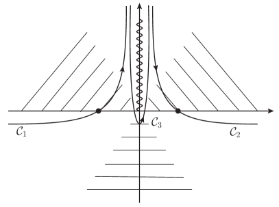
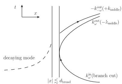
Figure 3: On the left: Contour of integration of Eq. (91) in the complex $k$-plane. The contributions of $\mathcal{C}_{1}$ and $\mathcal{C}_{2}$ can be evaluated by a saddle point approximation (the locations of the saddles $\pm k_{\rm saddle}$ are indicated by black dots). They give the two outgoing modes with high wave number. Instead the contribution of $\mathcal{C}_{3}$ is obtained by setting $d_{0}\to 0$, and gives the low wavenumber incoming branch. The hatched zones represent the directions in the complex plane where the integrand of Eq. (91) diverges for $|k|\to\infty$. The contours giving rise to physical modes will asymptote outside these zones.
On the right: the low frequency characteristics of the incoming mode $\phi_{\omega}^{\rm in}$ of Eq. (92). They approximatively describe the trajectories followed by the wave packets of Sec. III. For $|x|\gg d_{\rm broad}$, the mode is well approximated by a superposition of the 3 WKB modes of Eq. (94), the low wave number incoming one, and the two outgoing ones. For each mode, we give its root and the origin of its contribution to Eq. (91). See also Weinfurtner10 (Fig. 4), where these wave properties have been clearly observed.

References

- (1) R. Johnson, A modern introduction to the mathematical theory of water waves, vol. 19. Cambridge University Press, 1997.
- (2) G. Lawrence, “Steady flow over an obstacle,” J. Hydraul. Eng. 113 no. 8, (1987) 981–991.
- (3) T. Wu, “Generation of upstream advancing solitons by moving disturbances,” Journal of fluid mechanics 184 no. 75-99, (1987) 3.
- (4) S.-J. Lee, Generation of long water waves by moving disturbances. PhD thesis, California Institute of Technology, 1985.
- (5) J. Byatt-Smith, “The effect of laminar viscosity on the solution of the undular bore,” J. Fluid Mech 48 no. 1, (1971) 33–40.
- (6) G. El, R. Grimshaw, and A. Kamchatnov, “Analytic model for a frictional shallow-water undular bore,” CHAOS 15 (2005) 037102, nlin/0412061. http://arxiv.org/abs/nlin/0412061.
- (7) G. El, R. Grimshaw, and A. Kamchatnov, “Wave breaking and the generation of undular bores in an integrable shallow water system,” Studies in Applied Mathematics 114 no. 4, (2005) 395–411.
- (8) S. Hawking, “Particle Creation by Black Holes,” Commun. Math. Phys. 43 (1975) 199–220.
- (9) W. G. Unruh, “Notes on black-hole evaporation,” Phys. Rev. D 14 no. 4, (1976) 870–892.
- (10) W. Unruh, “Experimental black hole evaporation,” Phys. Rev. Lett. 46 (1981) 1351–1353.
- (11) W. Unruh, “Sonic analog of black holes and the effects of high frequencies on black hole evaporation,” Phys. Rev. D 51 (1995) 2827–2838.
- (12) R. Schutzhold and W. G. Unruh, “Gravity wave analogs of black holes,” Phys. Rev. D 66 (2002) 044019, arXiv:gr-qc/0205099 [gr-qc].
- (13) R. Balbinot, A. Fabbri, S. Fagnocchi, and R. Parentani, “Hawking radiation from acoustic black holes, short distance and back-reaction effects,” Riv. Nuovo Cim. 28 (2005) 1–55, arXiv:gr-qc/0601079 [gr-qc].
- (14) D. Acheson, “On over-reflexion,” J. Fluid Mech 77 no. 3, (1976) 433–472.
- (15) W. Greiner, “Quantum electrodynamics of strong fields,” Hadrons and Heavy Ions (1985) 95–226.
- (16) N. Birrell and P. Davies, Quantum fields in curved space. Cambridge University Press, 1984.
- (17) R. Brout, S. Massar, R. Parentani, and P. Spindel, “A Primer for black hole quantum physics,” Phys. Rept. 260 (1995) 329–454, arXiv:0710.4345 [gr-qc].
- (18) A. Fabrikant and I. Stepanyants, Propagation of waves in shear flows, vol. 18. World Scientific Publishing Company Incorporated, 1998.
- (19) S. Weinfurtner, E. W. Tedford, M. C. Penrice, W. G. Unruh, and G. A. Lawrence, “Measurement of stimulated Hawking emission in an analogue system,” Phys. Rev. Lett. 106 (2011) 021302, arXiv:1008.1911 [gr-qc].
- (20) S. Weinfurtner, E. W. Tedford, M. C. Penrice, W. G. Unruh, and G. A. Lawrenc, “Classical aspects of Hawking radiation verified in analogue gravity experiment,” arXiv:1302.0375 [gr-qc].
- (21) G. Rousseaux, C. Mathis, P. Maissa, T. G. Philbin, and U. Leonhardt, “Observation of negative phase velocity waves in a water tank: A classical analogue to the Hawking effect?,” New J.Phys. 10 (2008) 053015, arXiv:0711.4767 [gr-qc].
- (22) W. Unruh, “Irrotational, two-dimensional Surface waves in fluids,” arXiv:1205.6751 [gr-qc].
- (23) A. Coutant, A. Fabbri, R. Parentani, R. Balbinot, and P. R. Anderson, “Hawking radiation of massive modes and undulations,” Phys. Rev. D 86 (2012) 064022, arXiv:1206.2658 [gr-qc].
- (24) L. P. Pitaevskii, “Layered structure of superfluid 4 he with supercritical motion,” JETP Lett 39 no. 9, (1984) 423–425.
- (25) G. Baym and C. J. Pethick, “Landau critical velocity in weakly interacting bose gases,” 1206.7066. http://arxiv.org/abs/1206.7066.
- (26) E. Rolley, C. Guthmann, and M. Pettersen, “The hydraulic jump and ripples in liquid helium,” Physica B: Condensed Matter 394 no. 1, (2007) 46–55.
- (27) C. Mayoral, A. Recati, A. Fabbri, R. Parentani, R. Balbinot, and I. Carusotto, “Acoustic white holes in flowing atomic Bose-Einstein condensates,” New J. Phys. 13 (2011) 025007, arXiv:1009.6196 [cond-mat.quant-gas].
- (28) A. Coutant, R. Parentani, and S. Finazzi, “Black hole radiation with short distance dispersion, an analytical S-matrix approach,” Phys. Rev. D 85 (2012) 024021, arXiv:1108.1821 [hep-th].
- (29) F. Dalfovo, S. Giorgini, L. P. Pitaevskii, and S. Stringari, “Theory of Bose-Einstein condensation in trapped gases,” Rev. Mod. Phys. 71 (1999) 463–512.
- (30) J. Macher and R. Parentani, “Black hole radiation in Bose-Einstein condensates,” Phys. Rev. A 80 (2009) 043601, arXiv:0905.3634 [cond-mat.quant-gas].
- (31) M. W. Dingemans, Water wave propagation over uneven bottoms: Linear wave propagation, vol. 13. World Scientific, 1997.
- (32) C. C. Mei, The applied dynamics of ocean surface waves, vol. 1. World scientific, 1989.
- (33) J. Macher and R. Parentani, “Black/White hole radiation from dispersive theories,” Phys. Rev. D 79 (2009) 124008, arXiv:0903.2224 [hep-th].
- (34) S. Fulling, Aspects of Quantum Field Theory in Curved Space-Time, vol. 17. Cambridge University Press, 1989.
- (35) R. Brout, S. Massar, R. Parentani, and P. Spindel, “Hawking radiation without transPlanckian frequencies,” Phys. Rev. D 52 (1995) 4559–4568, arXiv:hep-th/9506121 [hep-th].
- (36) S. Finazzi and R. Parentani, “Hawking radiation in dispersive theories, the two regimes,” Phys.Rev. D85 (2012) 124027, arXiv:1202.6015 [gr-qc].
- (37) F. Michel and R. Parentani, “Saturation of black hole lasers in Bose-Einstein condensates,” Phys. Rev. D 88 (2013) 125012, arXiv:1309.5869 [cond-mat.quant-gas].
- (38) M. Abramowitz and I. Stegun, Handbook of mathematical functions with formulas, graphs, and mathematical tables, vol. 55. Dover publications, 1964.
- (39) S. Finazzi and R. Parentani, “Spectral properties of acoustic black hole radiation: broadening the horizon,” Phys. Rev. D 83 (2011) 084010, arXiv:1012.1556 [gr-qc].
- (40) V. Fleurov and R. Schilling, “Regularization of fluctuations near the sonic horizon due to the quantum potential and its influence on Hawking radiation,” Phys. Rev. A 85 (2012) 045602, arXiv:1105.0799 [cond-mat.quant-gas].
- (41) N. Van Kampen, Stochastic processes in physics and chemistry, vol. 1. North holland, 1992.
- (42) A. Coutant, Stability properties of Hawking radiation in the presence of ultraviolet violation of local Lorentz invariance. PhD thesis, Université Paris-Sud 11, 2012.
- (43) H. Lamb, Hydrodynamics. Cambridge University Press, 1993.
- (44) A. Coutant and R. Parentani, “Hawking radiation with dispersion: the broadened horizon paradigm,” arXiv:1402.2514 [gr-qc].
- (45) C. Barcelo, S. Liberati, and M. Visser, “Analogue gravity,” Living Rev. Rel. 8 (2005) 12, arXiv:gr-qc/0505065 [gr-qc].
- (46) T. Jacobson, “Black holes and Hawking radiation in spacetime and its analogues,” arXiv:1212.6821 [gr-qc].
- (47) J. Bognár, Indefinite inner product spaces. Springer New York, 1974.
- (48) T. Jacobson, “Black hole evaporation and ultrashort distances,” Phys. Rev. D 44 (1991) 1731–1739.
- (49) T. Jacobson, “Black hole radiation in the presence of a short distance cutoff,” Phys. Rev. D 48 (1993) 728–741, arXiv:hep-th/9303103 [hep-th].
- (50) S. Corley and T. Jacobson, “Hawking spectrum and high frequency dispersion,” Phys. Rev. D 54 (1996) 1568–1586, arXiv:hep-th/9601073 [hep-th].
- (51) S. Corley, “Computing the spectrum of black hole radiation in the presence of high frequency dispersion: An Analytical approach,” Phys. Rev. D 57 (1998) 6280–6291, arXiv:hep-th/9710075 [hep-th].
- (52) W. G. Unruh and R. Schutzhold, “On the universality of the Hawking effect,” Phys. Rev. D 71 (2005) 024028, arXiv:gr-qc/0408009 [gr-qc].
- (53) S. Robertson, Hawking Radiation in Dispersive Media. PhD thesis, University of St Andrews, 2011.
- (54) T. Jacobson and R. Parentani, “Black hole entanglement entropy regularized in a freely falling frame,” Phys. Rev. D 76 (2007) 024006, arXiv:hep-th/0703233 [hep-th].