Disordered topological metals

Abstract

Topological behavior can be masked when disorder is present. A topological insulator, either intrinsic or interaction induced, may turn gapless when sufficiently disordered. Nevertheless, the metallic phase that emerges once a topological gap closes retains several topological characteristics. By considering the self-consistent disorder-averaged Green function of a topological insulator, we derive the condition for gaplessness. We show that the edge states survive in the gapless phase as edge resonances and that, similar to a doped topological insulator, the disordered topological metal also has a finite, but non-quantized topological index. We then consider the disordered Mott topological insulator. We show that within mean-field theory, the disordered Mott topological insulator admits a phase where the symmetry-breaking order parameter remains non-zero but the gap is closed, in complete analogy to ‘gapless superconductivity’ due to magnetic disorder.

I Introduction

The discovery of topological insulators (TI) has brought us to nothing less than a revision of electronic band structure theory. Topological behavior was predicted for two-dimensional (2d) systems such as graphene with spin-orbit coupling Kane and Mele (2005, 2005) and HgTe quantum wells Bernevig et al. (2006). While the spin-orbit coupling in graphene turns out to be too weak, topological behavior has indeed been observed in HgTe/CdTe heterostructures König et al. (2007). Shortly thereafter, three-dimensional (3d) topological insulators were predicted to exist in bismuth alloys Moore and Balents (2007); Fu and Kane (2007); Fu et al. (2007), and by now have been discovered in a variety of materials (see, e.g., Refs. Neupane et al., 2012; Wang et al., 2011). From a theoretical perspective, these materials are described by a non-zero quantized topological index, which is essentially a generalization (albeit a nontrivial one) of the Chern number Volovik (2009); Moore and Balents (2007); Fu et al. (2007); Fu and Kane (2007); Qi et al. (2008); Wang et al. (2010). As in Hall insulators, the topological index implies the existence of protected edge/surface states at the boundaries of the system Volovik (2009); Gurarie (2011), which are responsible for a variety of exciting aspects of topological insulators. In two dimensions, the 1d edge states yield a quantized two-terminal conductance; in three dimensions, the 2d surface states consist of single helical Dirac cones, and gapping them leads to an anomalous surface Hall response and the so-called axion magneto-electric response Qi et al. (2008). The edge and surface states are at the heart of any possible technological application for topological insulators, including proposals to use them as a platform for Majorana states and quantum computation Fu and Kane (2008); Cook and Franz (2011); Fu and Kane (2009).

Alongside ideal TIs, recently, the study of the effects of imperfections – which plague essentially all realizations so far – has also picked up. Experimentally, already the 2d heterostructure realizations show the lack of quantized transport for samples of intermediate length König et al. (2007). Furthermore, 3d topological materials are often doped away from the bandgap, exhibiting a rather large bulk conductance Butch et al. (2010); Steinberg et al. (2010). Theoretical studies of doping showed that the metal obtained when the chemical potential of the TI lies outside the bandgap is characterized by a finite, but non-quantized topological index Barkeshli and Qi (2011); Bergman (2011); Bergman and Refael (2010); Hastings and Loring (2011); Loring and Hastings (2010). Studies of disorder led to additional surprises: it was shown that disorder can induce topological behavior in some trivial insulators Li et al. (2009); Groth et al. (2009); Guo et al. (2010), and (more importantly for the current work) that disorder may close the gap in topological insulators, leading to a metallic phase Shindou and Murakami (2009); Shindou et al. (2010); Prodan (2011); Leung and Prodan (2012).

In our work, we focus on the disorder-induced metallic phase in a simple test case of the Kane-Mele-Haldane honeycomb model Haldane (1988); Kane and Mele (2005). Naively, once the disorder destroys the gap of a topological insulator, a simple metal emerges. By first constructing the self-consistent disorder-averaged Green function, we investigate the disorder-averaged topological index as well as the fate of the edge states in the metallic phase. Our results indicate that, on both counts, the disorder-induced metal retains some signatures of its topological origin. Just like a doped TI, it has a non-quantized, but finite topological index. Correspondingly, we show that the edge states also survive as resonances of the disorder-averaged Green function. In particular, the edges states maintain their helical nature over a finite lifetime/mean free path, and then get absorbed into the bulk. Surprisingly, their velocity is strongly renormalized by the disorder, and vanishes at the transition between the insulating and metallic phase.

As pointed out by several groups, next-nearest neighbor interactions in various lattices may induce a topological phase Raghu et al. (2008); Weeks and Franz (2010); Zhang et al. (2009); Pesin and Balents (2010); Yang and Kim (2010), namely a so-called Mott topological insulator. Using our formalism, we self-consistently analyze the formation of such a phase in the honeycomb lattice. We show that, in close analogy to superconductivity in the presence of magnetic impurities Abrikosov and Gorkov (1961); de Gennes (1989); Maki (1969), disorder separates the appearance of topological order into two transitions: one associated with the appearance of a broken symmetry and an order parameter, and one (at larger interactions or weaker disorder) associated with the appearance of a spectral gap. The phase with a finite order parameter but no gap coincides with the topological metal we discussed before.

Below we start by developing the self-consistent disorder-averaged formalism (Sec. II), and use it to find the critical disorder strength for closing the TI’s band gap (Sec. III). We then proceed to analyze the topological index, following Volovik’s prescription (Sec. IV). Perhaps the most physical consequences of our discussion regard the edge states. In Sec. V we derive the properties of the edge states, assuming they correspond to a pole or resonance of the bulk disorder-averaged Green function when an edge is introduced. Before concluding, we discuss the possibility of an interaction-induced gapless topological phase in the disordered honeycomb lattice, and identify the parameter regime where this occurs (Sec. VI).

II Disorder-averaged Green function

We consider two copies of the Haldane Hamiltonian for a single-spin anomalous Hall state Haldane (1988) or, equivalently, the Kane-Mele model for spin-1/2 fermions Kane and Mele (2005). As we are interested in the low-energy physics, we restrict ourselves to the Hamiltonian near its Dirac nodes,

$${\cal{H}}=v_{F}k_{x}\sigma_{x}\tau_{z}-v_{F}k_{y}\sigma_{y}-\Delta\sigma_{z}s_{z}\tau_{z}.$$ (1)

Here $\sigma_{\alpha}$ are Pauli matrices acting in pseudo-spin (sublattice) space, while $\tau_{z}$ and $s_{z}$ are Pauli matrices operating in valley and spin space, respectively.

Our goal is to understand the properties of this model in the presence of disorder which, if sufficiently strong, destroys its gap. Impurity scattering is described by adding

$${\cal H}_{\rm imp}=\sum_{i,j,k}U_{ijk}({\bf k}-{\bf k^{\prime}})\sigma_{i}s_{j}\tau_{k},$$ (2)

with $\langle U_{ijk}({\bf r})\rangle=0$ and

$$\langle U_{ijk}({\bf r})U_{lmn}({\bf r^{\prime}})\rangle=\gamma_{ijk}\,\delta({\bf r}-{\bf r^{\prime}})\delta_{il}\delta_{jm}\delta_{kn},$$ (3)

to the Hamiltonian (1). Here $\langle\dots\rangle$ denotes disorder averaging.

Within the Born approximation, the self-energy due to impurity scattering reads

$$\Sigma(\omega) = \sum_{i,j,k}\gamma_{ijk}\,\sigma_{i}s_{j}\tau_{k}\int(dk)\;G_{0}(\omega,{\bf k})\,\sigma_{i}s_{j}\tau_{k},$$ (4)

where

$$G_{0}(\omega,{\bf k})=\left(i\omega-v_{F}(k_{x}\sigma_{x}\tau_{z}-k_{y}\sigma_{y})+\Delta\sigma_{z}s_{z}\tau_{z}\right)^{-1}$$ (5)

is the unperturbed imaginary-time Green function of the system and $(dk)=dk_{x}\,dk_{y}/(2\pi)^{2}$. Upon momentum integration, one obtains

$$\Sigma(\omega) = -\frac{1}{4\pi v_{F}^{2}}\ln\frac{D^{2}}{\omega^{2}+\Delta^{2}}\times$$

$$\times\sum_{i,j}\gamma_{ijk}\left[i\omega-\Delta(\sigma_{i}\sigma_{z}\sigma_{i})(s_{j}s_{z}s_{j})(\tau_{k}\tau_{z}\tau_{k})\right],$$

where $D$ is a high-energy cut-off of order of the bandwidth.

One may distinguish two types of disorder, $(\sigma_{i}\sigma_{z}\sigma_{i})(s_{j}s_{z}s_{j})(\tau_{k}\tau_{z}\tau_{k})=\pm\sigma_{z}s_{z}\tau_{z}$. The strongest effect on the gap is due to impurities that obey $(\sigma_{i}\sigma_{z}\sigma_{i})(s_{j}s_{z}s_{j})(\tau_{k}\tau_{z}\tau_{k})=\sigma_{z}s_{z}\tau_{z}$ which is the case, e.g., for relatively smooth potential disorder, $i=j=k=0$. Therefore, in the following, we will restrict our attention to this case.

To obtain the effective disorder-averaged Green function for this problem, we note that the self-energy renormalizes $\omega\rightarrow\tilde{\omega}$ and $\Delta\rightarrow\tilde{\Delta}$. The self-consistent Born approximation is obtained by substituting the renormalized $\tilde{\omega}$ and $\tilde{\Delta}$ in Eq. (II). The full Green function, $G^{-1}=G_{0}^{-1}-\Sigma$, can then be written in the form

$$G(\omega,{\bf k})=\left(i\tilde{\omega}-v_{F}(k_{x}\sigma_{x}\tau_{z}-k_{y}\sigma_{y})+\tilde{\Delta}\sigma_{z}s_{z}\tau_{z}\right)^{-1}\!,\!\!$$ (7)

where

$$\omega = \tilde{\omega}(1-\zeta\ln\frac{D^{2}}{\tilde{\omega}^{2}+\tilde{\Delta}^{2}}),$$ (8a)

$$\Delta = \tilde{\Delta}(1+\zeta\ln\frac{D^{2}}{\tilde{\omega}^{2}+\tilde{\Delta}^{2}}),$$ (8b)

with $\zeta=\gamma_{000}/({4\pi v_{F}^{2}})$, using the definition of $\gamma_{ijk}$ in Eq. (2).

In the absence of a topological insulator gap, $\Delta=0$, the above analysis readily yields the mean-free time. At $\tilde{\Delta}=\Delta=0$, analytic continuation of Eq. (8a) to real time yields

$$\omega=\tilde{\omega}\left(1-\zeta\ln\frac{D^{2}}{(i\tilde{\omega})^{2}}\right).$$ (9)

For $\omega=0$, we then obtain the mean free time Ostrovsky et al. (2006) at the Dirac point, $\tau=i/\tilde{\omega}(\omega=0)$. Namely,

$${\tau}^{-1}=De^{-\frac{1}{2\zeta}}.$$ (10)

III Gapless topological phase

As noted by several authors Shindou and Murakami (2009); Shindou et al. (2010); Hastings and Loring (2011); Loring and Hastings (2010); Prodan (2011); Leung and Prodan (2012), disorder produces a phase transition between the topological insulator phase and a gapless metallic phase. This can be seen most directly using the self-consistent Green function, given by Eqs. (7) and (8). In fact, the problem of finding the renormalized gap of the TI is equivalent to finding the renormalized gap of a superconductor with pair-breaking disorder. As explained in a review paper by Maki Maki (1969), upon analytic continuation to real frequencies, the renormalized gap may be identified as the largest $\omega$ which permits a real solution for the renormalized $\tilde{\omega}$ and $\tilde{\Delta}$. This follows from the expression for the density of states,

$$\nu(\omega) = -\frac{1}{8\pi}\textrm{Im}\left[\int(dk)\;{\rm Tr}\left[G(\omega,{\bf k})\right]_{i\omega\rightarrow\omega+i0^{+}}\right],$$ (11)

which upon using Eqs. (7) and (8a) yields

$$\nu(\omega)=\frac{1}{8v_{F}^{2}\zeta}\textrm{Im}\left[\tilde{\omega}\right].$$ (12)

Performing the analytic continuation and rescaling all energies by $\Delta$, Eqs. (8) simplify to

$$\frac{\omega}{\Delta} = \nu\left(1-\zeta\ln\frac{{\Lambda}^{2}}{\delta^{2}\!-\!\nu^{2}}\right),$$ (13a)

$$\delta^{-1} = 1+\zeta\ln\frac{{\Lambda}^{2}}{\delta^{2}\!-\!\nu^{2}},$$ (13b)

where $\delta=\tilde{\Delta}/\Delta$, $\nu=\tilde{\omega}/\Delta$, and $\Lambda=D/\Delta$. Combining the two equations, we can eliminate the logarithm to find

$$\frac{\omega}{\Delta}=\nu\left(2-\frac{1}{\delta}\right).$$ (14)

Solving Eq. (13b) for $\nu$ and inserting the solution into Eq. (14), we then obtain

$$\frac{\omega}{\Delta}=\left(2-\frac{1}{\delta}\right)\sqrt{\delta^{2}-{\Lambda}^{2}\exp\left[-\frac{1}{\zeta}\left(\frac{1}{\delta}-1\right)\right]},$$ (15)

which restricts the values of $\delta$ yielding $\omega\in{\mathbb{R}}_{+}$. On the one hand,

$$\delta>\delta_{\rm min}=\frac{1}{2},$$ (16)

and, on the other hand, in order for the square root to be real,

$$\delta<\delta_{\rm max}=\Lambda\exp\left[-\frac{1}{2\zeta}\left(\frac{1}{\delta_{\rm max}}-1\right)\right].$$ (17)

The gap is then a function of $\zeta$ and given by the maximum of $\omega$ for the range $\delta_{\rm min}\leq\delta\leq\delta_{\rm max}$.

At a critical value of the disorder parameter $\zeta$, the gap vanishes, and an insulator-metal transition occurs. This happens when $\delta_{\rm max}=\delta_{\rm min}=1/2$ and the two zeros of $\omega$ as a function of $\delta$ merge. One obtains

$$\frac{1}{2}=\Lambda e^{-\frac{1}{2\zeta_{\rm gap}}(2-1)}\quad\Rightarrow\quad\zeta_{\rm gap}=\frac{1}{2\ln(2\Lambda)},$$ (18)

or, equivalently,

$${\tau}_{\rm gap}^{-1}=\frac{\Delta}{2}$$ (19)

with $\tau$ given by Eq. (10), i.e., $\tau_{\rm gap}^{-1}=D\exp[-1/(2\zeta_{\rm gap})]$.

IV Topological index

We are interested in determining whether the system, though gapless, retains some topological properties. Let us start by considering the disorder-averaged topological index of the system. There are several definitions for the topological index in 2d Volovik (2009); Qi and Zhang (2011); Wang et al. (2010); Qi et al. (2008); Fu and Kane (2007). For our purposes, the most useful approach is the one of Volovik Volovik (2009); Qi et al. (2008); Qi and Zhang (2011) which calculates the Berry phase directly from the Green function. The expression for the topological index, see e.g. Eq. (48) in Ref. Qi and Zhang, 2011, for one spin species is given by

$$C = \frac{1}{2}\int d\omega\int(dk)\;\epsilon^{ij}{\rm Tr}\left[G\partial_{\omega}G^{-1}G\partial_{k_{i}}G^{-1}G\partial_{k_{j}}G^{-1}\right]_{\sigma,\tau}.$$ (20)

In order to obtain the disorder-averaged topological index, we simply substitute the disorder-averaged Green functions ft (1). Using Eq. (7), one obtains

$$G\partial_{\omega}G^{-1} = G\left(i\partial_{\omega}\tilde{\omega}+\partial_{\omega}\tilde{\Delta}\sigma_{z}s_{z}\tau_{z}\right)\!,\;\;$$ (21)

$$\epsilon^{ij}G\partial_{k_{i}}G^{-1}G\partial_{k_{j}}G^{-1} = iv_{F}^{2}G\sigma_{y}\left\{\sigma_{z}\tau_{z},G\right\}\sigma_{y}.$$ (22)

Evaluating the $k$-integrals and the trace, the expression can be reduced to

$$C = \frac{1}{\pi}s_{z}\int d\omega\;\left(\tilde{\omega}\partial_{\omega}\tilde{\Delta}-\tilde{\Delta}\partial_{\omega}\tilde{\omega}\right)\frac{1}{\tilde{\omega}^{2}+\tilde{\Delta}^{2}}.$$ (23)

Thus, one obtains

$$C = -\frac{2}{\pi}s_{z}\arctan\frac{1}{x_{\rm min}},$$ (24)

where

$$x_{\rm min} = \frac{\tilde{\omega}(\omega=0)}{\tilde{\Delta}(\omega=0)}=\textrm{Re}\left[\sqrt{4\frac{D^{2}}{\Delta^{2}}e^{-\frac{1}{\zeta}}-1}\,\right],$$ (25)

or, using the mean free time,

$$x_{\rm min} = \theta\left(1-\frac{\Delta}{2}\tau\right)\sqrt{\left(\frac{\Delta}{2}\tau\right)^{-2}-1}.$$ (26)

In the gapped region, $\tau^{-1}<\tau_{\rm gap}^{-1}=\Delta/2$, one obtains $x_{\rm min}=0$ and therefore the topological constant is $C=-s_{z}$. By contrast, if $\Delta=0$, one obtains $x_{\rm min}=\infty$ and therefore the topological constant vanishes, $C=0$. The gapless region at $\tau^{-1}>\tau_{\rm gap}^{-1}$, however, emerges as the most interesting. In this region $C$ changes smoothly from $-s_{z}$ to $0$ (see Fig. 1). Close to the closing of the gap, $0<\tau^{-1}-\tau_{\rm gap}^{-1}\ll\tau_{\rm gap}^{-1}$, we find

$$\delta C=C+s_{z}\propto\sqrt{\tau_{\rm gap}/\tau-1},$$ (27)

whereas deep in the gapless phase, $\tau^{-1}\gg\tau_{\rm gap}^{-1}$ we find that the index falls off as

$$C\propto\tau/\tau_{\rm gap}.$$ (28)

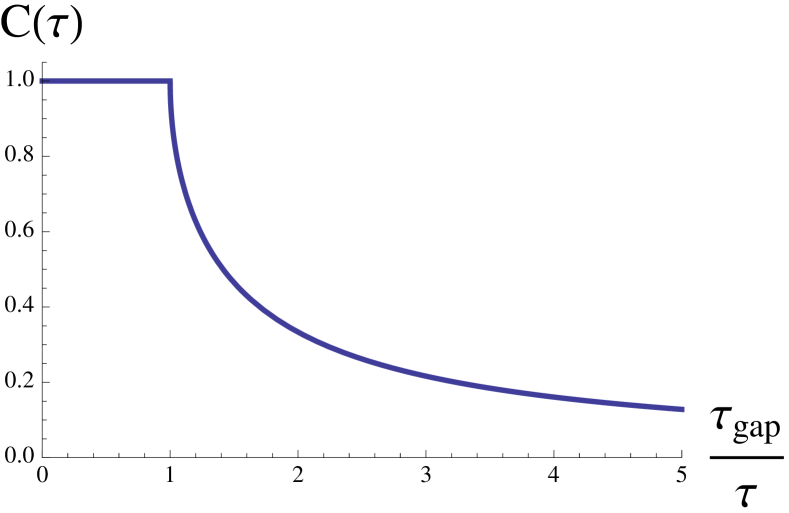
Figure 1: The topological index for $s_{z}=-1$ as a function of the scattering rate $1/\tau$. As soon as $1/\tau$ exceeds $1/\tau_{\rm gap}=\Delta/2$, the topological index plunges from a quantized value to a nonquantized and monotonically decreasing, disorder-dependent value.

A non-quantized topological index requires a bit of consideration. For a given realization, by definition, Eq. (20) yields a quantized value. However, in the gapless phase, this value would fluctuate between 0 and $-s_{z}$, depending on the specific disorder realization. Upon averaging, one may, thus, obtain a non-quantized value. It has already been pointed out by Loring and Hastings Hastings and Loring (2011); Loring and Hastings (2010), that the average topological index of doped 2d TIs interpolates continuously between the respective quantized values in the topologically non-trivial and trivial phases as the chemical potential is varied and the valence band becomes partially filled. Non-quantized values have also been obtained in clean 3d topological insulators, when the chemical potential is within the valence or conduction band Barkeshli and Qi (2011); Bergman (2011).

The calculation we presented above fits well with the idea of a partial response of a metal. It shows that the disorder-induced gapless state should be quite similar in its behavior to a doped topological insulator, with the chemical potential lying within one of the bands. The index itself, however, is not a measurable quantity. Below, we try to understand the physical ramifications of this partial topological behavior in terms of the edge state physics.

V The fate of the edge state

In the search for topological properties of the disordered metal, several works direct us to the edge states. Recently Ref. Gurarie, 2011 confirmed rigorously that a spatial jump of the topological index (defined by Eq. (20)) results in an edge state, i.e., a pole ft (2) of the Green function at the location of the jump. It is natural to ask what a non-quantized jump implies for such edge states?

Indeed, given the connections above, we speculate that the non-quantized topological index implies an edge state resonance of the Green function, but with a finite lifetime due to hybridization with the continuum.

To explore the edge physics, we start with the inverse of the disorder-averaged Green function Eq. (7) which may be associated with an effective Schrödinger equation. For the four-component wave function $\psi_{s_{z}}$ of a given spin species, the effective Schrödinger equation reads

$$\left(v_{F}k_{x}\sigma_{x}\tau_{z}-v_{F}k_{y}\sigma_{y}-\tilde{\Delta}\sigma_{z}s_{z}\tau_{z}\right)\psi_{s_{z}}=\tilde{\omega}\psi_{s_{z}}.$$ (29)

Consider now that the system occupies the half-plane $x<0$. To satisfy the boundary conditions, we have to find solutions of (29) that vanish on the edge, $x=0$. We recall that the degree of freedom $\tau_{z}=\pm 1$ indicates the valley, i.e., the momentum around which $k_{x},\,k_{y}$ in the Hamiltonian (29) are measured. The true momenta are $p_{x}=k_{x}+\tau_{z}K_{0}$ and $p_{y}=k_{y}$, where $K_{0}=4\pi/(3\sqrt{3}a)$ and $a$ is the lattice spacing. For the edge state to obey the boundary conditions, it is necessary to mix wave functions from the two valleys. Namely, the generic form of the edge-state wave function, assuming it is given by a simple superposition of momentum states (albeit with complex momenta), is $\psi=\sum_{\tau_{z}=\pm 1}\psi_{\tau_{z}}(x,y)e^{i\tau_{z}K_{0}x}$. This implies that, for the wave function to vanish at the edge, both components $\tau_{z}=\pm 1$ of the wave function must be described by identical sublattice ($\sigma$-space) spinors.

To find such solutions, we separate the Schrödinger equation into its parts dependent and independent of $\tau_{z}$, and require that both vanish. Namely,

$$\left(v_{F}k_{x}\sigma_{x}-\tilde{\Delta}\sigma_{z}s_{z}\right)\phi_{s_{z}} = 0,$$ (30a)

$$\left(\tilde{\omega}+v_{F}k_{y}\sigma_{y}\right)\phi_{s_{z}} = 0,$$ (30b)

where $\phi_{s_{z}}$ is a two-component wave function in sublattice space. In order for these equations to be solvable simultaneously, $k_{x}$ and $k_{y}$ must obey

$$k_{x}=\pm is_{z}\frac{\tilde{\Delta}}{v_{F}}\qquad{\rm and}\qquad k_{y}=\mp\frac{\tilde{\omega}}{v_{F}},$$ (31)

while the corresponding wave functions take the form $\phi_{s_{z}}=(1,\pm i)^{T}/\sqrt{2}$.

The complex valued momentum $k_{x}$ describes the decay of the edge state away from the edge. The decay length scale is, therefore, given by $L_{\perp}=v_{F}/\textrm{Re}[\tilde{\Delta}]$. The sign has to be chosen such that $\textrm{Im}[k_{x}]<0$. As can be seen in Fig. 2, the state remains well localized on the edge. Namely, the transverse localization length only increases from $L_{\perp}=v_{F}/\Delta$ at $\zeta=0$ to $L_{\perp}=2v_{F}/\Delta$ in the gapless phase.

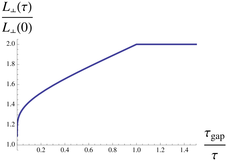
Figure 2: Penetration of the edge state into the bulk: The transverse localization length of the edge state, $L_{\perp}(\tau)=v_{F}/\textrm{Re}[\tilde{\Delta}]$, in units of the bare decay length, $L_{\perp}(0)=v_{F}/\Delta$, is plotted as a function of disorder. It varies by a factor of $2$.

The momentum $k_{y}$ describes the propagation along the edge. The appropriate choice of sign for $k_{x}$ yields $k_{y}=-s_{z}\tilde{\omega}/v_{F}$. Thus, as expected, the sign of $k_{y}$ and therefore the propagation direction is tied to the spin. To obtain the dispersion of the edge states, as well as their lifetime, we need to find the relation between $k_{y}$ and the real energy $\omega$. We use Eqs. (8) to write

$$\omega=\tilde{\omega}\left(1-\zeta\ln\frac{D^{2}(2\tilde{\omega}-\omega)^{2}}{\tilde{\omega}^{2}(\Delta^{2}-(2\tilde{\omega}-\omega)^{2})}\right).$$ (32)

Since the edge state is helical, an imaginary part of the wave number $k_{y}$ can be interpreted as a finite lifetime of the state. To illustrate this, consider the simplest Schrödinger equation for a decaying helical mode: $i\frac{\partial\psi}{\partial t}=-v\frac{1}{i}\frac{\partial\psi}{\partial x}-i\frac{\psi}{\tau}$. This is equivalently solved either by $\psi=\exp[i\omega(t-x/v)-t/\tau]$ or $\psi=\exp[i\omega(t-x/v)-x/(v\tau)]$. Which of these two solutions should be used depends on the specific situation, and, for a Green-function description, the two should be equivalent.

(a)

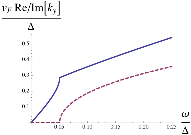
(b)

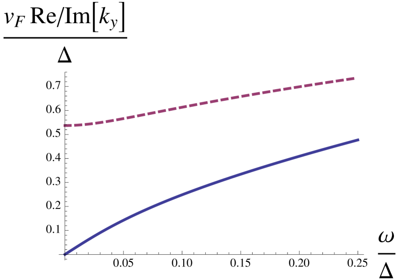
Figure 3: Dispersion of the edge states: $k_{\parallel}=\textrm{Re}[\tilde{\omega}]/v_{F}$ (full line) and inverse decay length $L_{\parallel}^{-1}=\textrm{Im}[\tilde{\omega}]/v_{F}$ (dashed line) versus $\omega$. (a) Gapped phase ($\zeta=0.8\,\zeta_{\rm gap}$). (b) Gapless phase ($\zeta=1.2\,\zeta_{\rm gap}$).

When the disorder is sufficiently weak, $\zeta<\zeta_{\rm gap}$, the dispersion decribed by (32) can be separated into two regimes. At energies below the renormalized gap edge, $\omega<E_{\rm gap}<\Delta$, we find edge state solutions that do not decay, i.e., $\textrm{Im}[\tilde{\omega}]=0$. By contrast, at energies $\omega>E_{\rm gap}$, we find edge states with a finite lifetime, $\textrm{Im}[\tilde{\omega}]\neq 0$. Indeed, the finite lifetime of the edge state is a consequence of the hybridization with the continuum which permits for the state to decay to extended bulk states. The dispersion and lifetime of the weak-disorder edge states is shown in Fig. 3a.

As the disorder increases, $\zeta>\zeta_{\rm gap}$, the bandgap vanishes. Now the entire edge state branch is hampered by a finite lifetime and propagation length, see Fig. 3b. The decay length in the propagation direction $L_{\parallel}$ is nearly independent of energy, but depends strongly on the disorder strength. By setting $\omega=\textrm{Re}[\tilde{\omega}]=0$, one can obtain $L_{\parallel}=v_{F}/\textrm{Im}[\tilde{\omega}]$. We find, relying on the identification of $k_{y}$ in Eq. (31),

$$L_{\parallel}^{-1}=\frac{1}{v_{F}\tau}\sqrt{1-\left(\frac{\Delta}{2}\tau\right)^{2}},$$ (33)

where $\tau$ is the mean free time as defined in Eq. (10). The result is shown in Fig. 4. At $\zeta=\zeta_{\rm gap}$, the decay length diverges, $L_{\parallel}\rightarrow\infty$.

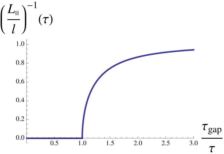
Figure 4: Inverse decay length along the edge, $L_{\parallel}^{-1}$, in units of the inverse bulk mean free path, $l^{-1}=1/(v_{F}\tau)$, as a function of disorder. $L_{\parallel}^{-1}$ is zero in the gapped phase and approaches $l^{-1}$ as $\tau^{-1}\rightarrow\infty$.

Quite interestingly, the survival length of the edge state is closely related to the topological index calculated in Sec. IV. Namely,

$$C=-\frac{2}{\pi}s_{z}\arctan\frac{L_{\parallel}\Delta}{2v_{F}}.$$ (34)

This gives more ground to the speculation that a non-quantized topological index will always be associated with a finite lifetime for the edge states.

Another interesting property of the edge states is the propagation velocity, $v=v_{F}(\partial\omega/\partial\tilde{\omega})$. In the limit $\omega\rightarrow 0$, straightforward manipulation of Eq. (32) leads to

$$\frac{v}{v_{F}}=\left\{\begin{array}[]{cc}1-2\zeta\ln\frac{D(2-\frac{v}{v_{F}})}{\Delta}&\zeta<\zeta_{c},\\[2.84544pt] \frac{2v_{F}^{2}\tau^{2}L_{\parallel}^{-2}}{\zeta^{-1}-\left(\frac{\Delta}{2}\tau\right)^{2}}&\zeta>\zeta_{c}.\end{array}\right.$$ (35)

The result is depicted in Fig. 5a. Approaching the transition from both sides, we find that the velocity vanishes when $\zeta=\zeta_{\rm gap}$. In the gapped regime, we identify the transcendental equation defining $v$ for $\zeta<\zeta_{\rm gap}$ as reducing to the gaplessness condition (18) upon setting $v=0$. Indeed, the edge velocity is suppressed throughout the weak-disorder regime at energies tending to the gap from below, $\omega\rightarrow E_{\rm gap}^{-}$. In the gapless regime, $\zeta>\zeta_{\rm gap}$, the denominator ft (3) in Eq. (35) is regular at $\zeta=\zeta_{\rm gap}$. Thus, since $L_{\parallel}^{-1}$ vanishes at the transition, so does $v$.

(a)

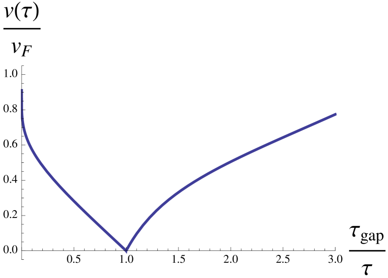
(b)

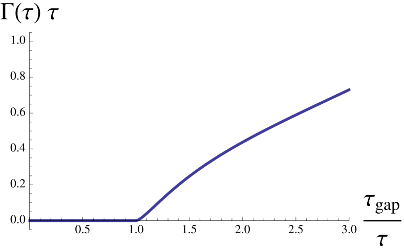
Figure 5: Properties of the edge states as a function of the scattering rate $\tau^{-1}$. (a) Effective velocity $v$ of the edge states in units of the Fermi velocity. (b) Decay rate $\Gamma$ of the edge states in units of the scattering rate $\tau^{-1}$. As the velocity vanishes at $\zeta_{\rm gap}$, $\Gamma$ increases at a much slower rate than $L_{\parallel}^{-1}$ in the gapless phase, namely $\Gamma\propto L_{\parallel}^{-3}$.

With the velocity and the decay length, we may now identify the decay rate of the edge states in the gapless regime as a function of disorder,

$$\Gamma=\frac{v}{L_{\parallel}}=\frac{2v_{F}^{3}\tau^{2}L_{\parallel}^{-3}}{\zeta^{-1}-\left(\frac{\Delta}{2}\tau\right)^{2}}.$$ (36)

Thus the lifetime $\sim\Gamma^{-1}$ diverges at the point where the gap closes, and follows the third power of the decay length as disorder further grows (the result is depicted in Fig. 5b).

VI Topological Mott metal

Topological behavior may also emerge due to electron-electron interactions rather than a native spin-orbit coupling and band inversionRaghu et al. (2008); Weeks and Franz (2010); Zhang et al. (2009); Pesin and Balents (2010); Yang and Kim (2010). Under these circumstances, it is particularly interesting to ask whether a gapless topological phase can exist when the disorder is strong. The situation is rather reminiscent of the competition between magnetic impurities and s-wave superconductivity. It is well known that magnetic impurities may induce a phase which is s-wave superconducting, albeit gapless Abrikosov and Gorkov (1961); de Gennes (1989); Maki (1969). Namely, the disorder suppresses both the order parameter and the spectral gap, but the two do not vanish simultaneously. In the gapless phase, while the material has a superconducting stiffness, its critical current is suppressed. In this section, we will establish that interacting systems can host a gapless topological phase as well, albeit in a rather narrow range of interactions and disorder.

The idea of an interaction-induced topological insulator, i.e., a topological Mott insulator, was first explored in Ref. Raghu et al., 2008 for the case of a honeycomb lattice. It was shown that a next-nearest neighbor interaction may open a gap which has opposite sign at the two Dirac nodes of the band structure. Using the Hartree-Fock approach this can be analyzed self-consistently, which is the approach we will pursue below. Later work Weeks and Franz (2010) demonstrated that various lattice structures may also be susceptible to competing symmetry-broken phases, most notably the Kekule phase in the honeycomb lattice. We will stir clear of the possibility of competing phases, and concentrate on the range of parameters most conducive to the formation of topological order.

In particular, we will consider a honeycomb lattice in 2d with next-nearest neighbor repulsion of strength $V$. Our starting point is the tight-binding Hamiltonian,

$$H = -t\sum_{\langle i,j\rangle;\sigma}(c_{i\sigma}^{\dagger}c_{j\sigma}+{\rm h.c.})$$

$$+V\sum_{\langle\langle i,j\rangle\rangle}\left(\sum_{\sigma}c_{i\sigma}^{\dagger}c_{i\sigma}-1\right)\left(\sum_{\sigma}c_{j\sigma}^{\dagger}c_{j\sigma}-1\right).$$

To this Hamiltonian, we will add disorder as explained in Eq. (2).

VI.1 Self-consistent Hartree-Fock analysis

The symmetry breaking that leads to topological behavior in the honeycomb lattice occurs on the next-nearest neighbor bonds. The next-nearest neighbor hopping may acquire an imaginary expectation value which will then result in the Haldane model for each spin flavor. A next-nearest neighbor interaction naturally leads to such a broken symmetry Raghu et al. (2008); Weeks and Franz (2010). The interaction term may be decoupled using a Hubbard-Stratonovich transformation, yielding the mean-field Hamiltonian,

$$H=-t\sum_{\langle i,j\rangle;\sigma}(c_{i\sigma}^{\dagger}c_{j\sigma}\!+\!{\rm h.c.})-2V\!\!\!\!\!\sum_{\langle\langle i,j\rangle\rangle;\sigma,\sigma^{\prime}}\!\!\!\!\!\chi_{ij}^{\sigma\sigma^{\prime}}c_{i\sigma}^{\dagger}c_{j\sigma^{\prime}},$$ (38)

together with the self-consistency equation,

$$\chi_{ij}^{\sigma\sigma^{\prime}}=\langle c_{j\sigma^{\prime}}^{\dagger}c_{i\sigma}\rangle.$$ (39)

After Fourier transformation, the Hamiltonian in the sublattice (pseudo-spin) basis takes the form

$$H = -\sum_{{\bf k},{\bf k}^{\prime};\sigma,\sigma^{\prime}}C_{{\bf k}\sigma}^{\dagger}\begin{pmatrix}\Delta_{A}^{\sigma\sigma^{\prime}}({\bf k},{\bf k^{\prime}})&2t\sum_{l}e^{-i{\bf ka}_{l}}\delta_{{\bf k},{\bf k}^{\prime}}\delta_{\sigma\sigma^{\prime}}\\ 2t\sum_{l}e^{i{\bf ka}_{l}}\delta_{{\bf k},{\bf k}^{\prime}}\delta_{\sigma\sigma^{\prime}}&\Delta_{B}^{\sigma\sigma^{\prime}}({\bf k},{\bf k^{\prime}})\end{pmatrix}C_{{\bf k}^{\prime}\sigma^{\prime}},$$ (40)

where $\Delta^{\sigma\sigma^{\prime}}_{X,ij}=2V\chi^{\sigma\sigma^{\prime}}_{X,ij}$ and $X=A,\,B$ is the sublattice index. Furthermore, ${\bf a}_{l}$ (with $l=1,2,3$) are the lattice vectors of the honeycomb lattice, connecting the $A$ and $B$ sublattices.

At low energies, we assume that the interaction opens a topological insulator gap without breaking time-reversal symmetry, and therefore $\Delta$ has the form

$$\Delta_{X}^{\sigma\sigma^{\prime}}({\bf k},{\bf k^{\prime}})=\Delta\,{\rm sign}({k_{x}})(-1)^{X+\sigma}\delta_{{\bf k},{\bf k}^{\prime}}\delta_{\sigma\sigma^{\prime}}$$ (41)

with $(-1)^{A/B}=\pm 1$. Note that ${\rm sign}(k_{x})$ inherits the valley index, and therefore in a continuum picture will be replaced by $\tau_{z}$. Indeed, the low-energy Hamiltonian of the system, upon linearization of the dispersion near the nodes, reads

$${\cal H}=v_{F}k_{x}\sigma_{x}\tau_{z}-v_{F}k_{y}\sigma_{y}-\Delta\sigma_{z}s_{z}\tau_{z},$$ (42)

which is the same as Eq. (1). However, this Hamiltonian is now supplemented by the self-consistency condition for $\Delta$. Assuming that the low-energy part of the dispersion is dominant in determining the self-consistent bond order parameter, the self-consistency condition takes the form

$$\Delta = V\int\frac{d\omega}{2\pi}\int(dk)\;{\rm Tr}\left[G(\omega,{\bf k})\sigma_{z}s_{z}\tau_{z}\right]$$ (43)

with $G(\omega,{\bf k})$ given by Eq. (7).

VI.2 Finding the critical disorder and interaction

Disorder now has two effects. As before, it suppresses the spectral gap, but, at the same time, it also affects the order parameter: for any interaction strength which leads to the topological phase, adding sufficiently strong disorder will destroy that phase. The condition for the spectral gap to vanish remains the same as before. Namely,

$$\zeta_{\rm gap}=\frac{1}{2\ln\left(2\frac{D}{\Delta}\right)},$$ (44)

see Eq. (18). However, $\Delta=\Delta(\zeta_{\rm gap})$ has now to be determined self-consistently. Substituting the Green function, Eq. (7), into the self-consistency condition (43), we find

$$\Delta = 8V\int\frac{d\omega}{2\pi}\int(dk)\;\left[\frac{\tilde{\Delta}}{\tilde{\omega}^{2}+v_{F}^{2}k^{2}+\tilde{\Delta}^{2}}\right],$$ (45)

which, upon performing the momentum integration and using Eqs. (8), reduces to

$$\Delta = \frac{c}{\zeta\Lambda}\int\limits_{0}^{\Lambda}d\omega\;(1-\delta),$$ (46)

with $c=2VD/(\pi^{2}v_{F}^{2})$, and $\Lambda=D/\Delta$ as defined earlier. Note that $\delta$ and $\omega$ are related through Eq. (15).

Fig. 6 shows the order parameter $\Delta_{0}$ in the absence of disorder. To obtain the critical disorder strength, $\zeta_{c}$, for which the topological phase is destroyed, we replace the $\omega$-integral with an integral over $\delta$ and let $\delta/\Lambda\rightarrow 0$. The result is a transcendental equation that connects $c$ and $\zeta_{c}$,

$$1 = \frac{ce^{-\frac{1}{2\zeta_{c}}}}{\zeta_{c}}\int\limits_{1/2}^{1}d\delta\left(2\!-\!\frac{1}{\delta}\right)e^{-\frac{1}{2}\zeta_{c}^{-1}(\delta^{-1}-2)}.$$ (47)

The critical scattering rate $1/\tau_{c}$ as a function of $c$ is plotted in Fig. 6.

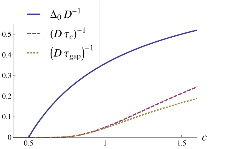
Figure 6: Order parameter in the absence of disorder, $\Delta_{0}/D$, and critical scattering rates, $1/(D\tau_{c})$ (vanishing of the order parameter) and $1/(D\tau_{\rm gap})$ (vanishing of the spectral gap), as a function of interaction strength, $c$.

VI.3 Disorder threshold for gaplessness

To obtain the disorder strength, $\zeta_{\rm gap}$, where the spectral gap vanishes, we need to combine Eqs. (43) and (46). We find another transcendental equation for $\zeta_{\rm gap}$,

$$1=\frac{ce^{-\frac{1}{2\zeta_{\rm gap}}}}{\zeta_{\rm gap}}\int\limits_{1/2}^{1}d\delta\left(2\!-\!\frac{1}{\delta}\right)\sqrt{e^{-\zeta_{\rm gap}^{-1}(\delta^{-1}-2)}\!-\!4\delta^{2}}.$$ (48)

The result is plotted in Fig. 6. Furthermore, the width of the gapless regime is shown in Fig. 7. The larger $c$ and thus $\Delta_{0}$, the larger the regime where the order parameter survives while the gap is closed. In the gapless regime $\zeta_{\rm gap}<\zeta<\zeta_{c}$, the above considerations about the topological index and edge states remain valid, i.e., the system is a topological Mott metal.

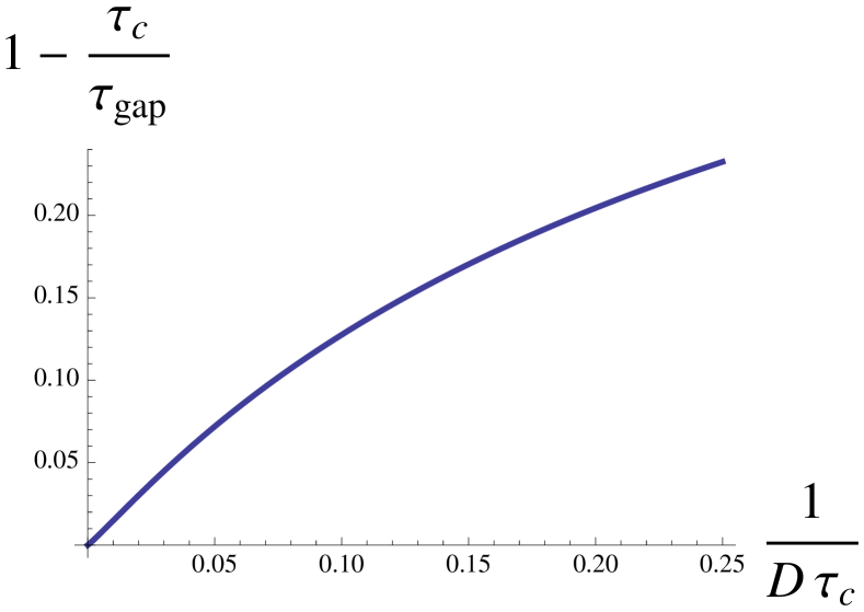
Figure 7: Region of gaplessness at $T=0$: $(\tau_{c}^{-1}-\tau_{\rm gap}^{-1})/\tau_{c}^{-1}$ as a function of $1/(D\tau_{c})$.

VII Conclusions

We have studied the disorder-induced gapless phase of a 2d topological insulator system. In particular, we have concentrated on (i) the Kane-Mele model, which is intrinsically topological, as well as (ii) an example of a Mott topological insulator, namely graphene with next-nearest neighbor interactions that induce a topological phase.

Our main conclusion is that the disorder-induced gapless system remains topologically non-trivial. Naively, one would think that once the gap of a topological insulator is closed, its topological properties also vanish. Nevertheless, it appears that the gapless phase retains evidence of its topological origin. Namely, the gapless phase is characterized by a finite, yet non-quantized disorder-averaged topological index. This is reminiscent of doped topological insulators for which Refs. Hastings and Loring, 2011; Loring and Hastings, 2010 showed that the topological index changes continuously between 1 and 0 when the chemical potential is sweeped between the top and bottom of the valence band.

In addition, we find that the gapless phase still supports helical edge states, though with a finite lifetime and a renormalized velocity. This is consistent with the findings of Ref. Bergman and Refael, 2010, where a bulk parasitic metal overlapping with edge states was considered in the clean case. There the individual orbitals of the edges states which overlap in both momentum and energy with bulk states are split into two states, with energies above and below the parasitic metallic band. However, these states leave a ‘ghost’ behind: an edge state with a finite lifetime, which appears as a resonance in the Green function of the system, although not being an exact eigenstate of the Hamiltonian. Furthermore, the finding of a finite lifetime limiting the manifestations of topological effects may be related to the ‘parity diffusion mode’ found in Ref. Shindou and Murakami, 2009 (see, e.g., Eqs. (4) and (66) ibid., where the IR cutoff indicates a finite lifetime). Since that work considered disordered 3d TIs, a direct comparison, however, is not possible.

The properties of the edge states/resonances have additional features worth mentioning. First, it appears that a close link exists between the decay length of the edge resonances and the non-quantized topological index, as shown in Eq. (34). Next, disorder strongly affects the edge state velocity. Weak disorder suppresses the edge velocity, until it vanishes at the disorder strength where the gap closes. This is essentially dictated by the fact that the helical edge branch is confined between the top of the valence band and the bottom of the conduction band. Interestingly, the velocity picks up as a function of disorder in the gapless regime, as shown in Fig. 5b. The suppression of the velocity when $\zeta\sim\zeta_{\rm gap}$ implies that an electron tunneling into the surface will remain near the point of tunneling for an extended time. This effect could be observed through an enhanced zero-bias anomaly due to a temporary Coulomb blockade Altshuler and Aronov (1979); Altshuler et al. (1980); Kane and Fisher (1992).

If the topological phase is induced by interactions, as considered in the last part of the paper, the disorder affects both the excitation gap and the order parameter. In analogy with gapless superconductivity, we have shown that there is a range of disorder strengths where a gapless topological phase is realized. In this regime, the disorder fully suppresses the gap, whereas a finite order parameter prevails up to a critical disorder strength. Within this range, the material will have the same properties as the non-interacting disorder-induced gapless topological phase.

We acknowledge helpful discussions with Victor Gurarie, Doron Bergman, and Matt Hastings. This work was funded through an EU-FP7 Marie Curie IRG (JM), and by DARPA and FENA (GR), the Humboldt foundation, and the IQIM, an NSF Physics Frontiers Center with support of the Gordon and Betty Moore Foundation. We also thank the Aspen Center for Physics, where part of the work was done.

References

- Kane and Mele (2005) C. L. Kane and E. J. Mele, Physical Review Letters, 95, 226801 (2005a), arXiv:cond-mat/0411737 .
- Kane and Mele (2005) C. L. Kane and E. J. Mele, Physical Review Letters, 95, 146802 (2005b), arXiv:cond-mat/0506581 .
- Bernevig et al. (2006) B. A. Bernevig, T. L. Hughes, and S.-C. Zhang, Science, 314, 1757 (2006), arXiv:cond-mat/0611399 .
- König et al. (2007) M. König, S. Wiedmann, C. Brüne, A. Roth, H. Buhmann, L. W. Molenkamp, X.-L. Qi, and S.-C. Zhang, Science, 318, 766 (2007).
- Moore and Balents (2007) J. E. Moore and L. Balents, Phys. Rev. B, 75, 121306 (2007), arXiv:cond-mat/0607314 .
- Fu and Kane (2007) L. Fu and C. L. Kane, Phys. Rev. B, 76, 045302 (2007), arXiv:cond-mat/0611341 .
- Fu et al. (2007) L. Fu, C. L. Kane, and E. J. Mele, Physical Review Letters, 98, 106803 (2007), arXiv:cond-mat/0607699 .
- Neupane et al. (2012) M. Neupane, S.-Y. Xu, L. A. Wray, A. Petersen, R. Shankar, N. Alidoust, C. Liu, A. Fedorov, H. Ji, J. M. Allred, Y. S. Hor, T.-R. Chang, H.-T. Jeng, H. Lin, A. Bansil, R. J. Cava, and M. Z. Hasan, ArXiv e-prints (2012), arXiv:1206.0695 .
- Wang et al. (2011) Y. J. Wang, H. Lin, T. Das, M. Z. Hasan, and A. Bansil, New Journal of Physics, 13, 085017 (2011), arXiv:1106.3316 .
- Volovik (2009) G. E. Volovik, The Universe in a Helium Droplet (Oxford University Press, USA, 2009).
- Qi et al. (2008) X.-L. Qi, T. L. Hughes, and S.-C. Zhang, Phys. Rev. B, 78, 195424 (2008), arXiv:0802.3537 .
- Wang et al. (2010) Z. Wang, X.-L. Qi, and S.-C. Zhang, New Journal of Physics, 12, 065007 (2010), arXiv:0910.5954 .
- Gurarie (2011) V. Gurarie, Phys. Rev. B, 83, 085426 (2011), arXiv:1011.2273 .
- Fu and Kane (2008) L. Fu and C. L. Kane, Physical Review Letters, 100, 096407 (2008), arXiv:0707.1692 .
- Cook and Franz (2011) A. Cook and M. Franz, Phys. Rev. B, 84, 201105 (2011), arXiv:1105.1787 .
- Fu and Kane (2009) L. Fu and C. L. Kane, Physical Review Letters, 102, 216403 (2009), arXiv:0903.2427 .
- Butch et al. (2010) N. P. Butch, K. Kirshenbaum, P. Syers, A. B. Sushkov, G. S. Jenkins, H. D. Drew, and J. Paglione, Phys. Rev. B, 81, 241301 (2010), arXiv:1003.2382 .
- Steinberg et al. (2010) H. Steinberg, D. R. Gardner, Y. S. Lee, and P. Jarillo-Herrero, ArXiv e-prints (2010), arXiv:1003.3137 .
- Barkeshli and Qi (2011) M. Barkeshli and X.-L. Qi, Physical Review Letters, 107, 206602 (2011), arXiv:1101.3104 .
- Bergman (2011) D. L. Bergman, Physical Review Letters, 107, 176801 (2011), arXiv:1101.4233 .
- Bergman and Refael (2010) D. L. Bergman and G. Refael, Phys. Rev. B, 82, 195417 (2010), arXiv:1003.3018 .
- Hastings and Loring (2011) M. B. Hastings and T. A. Loring, Annals of Physics, 326, 1699 (2011), arXiv:1012.1019 .
- Loring and Hastings (2010) T. A. Loring and M. B. Hastings, EPL (Europhysics Letters), 92, 67004 (2010), arXiv:1005.4883 .
- Li et al. (2009) J. Li, R.-L. Chu, J. K. Jain, and S.-Q. Shen, Physical Review Letters, 102, 136806 (2009), arXiv:0811.3045 .
- Groth et al. (2009) C. W. Groth, M. Wimmer, A. R. Akhmerov, J. Tworzydlo, and C. W. J. Beenakker, Physical Review Letters, 103, 196805 (2009), arXiv:0908.0881 .
- Guo et al. (2010) H.-M. Guo, G. Rosenberg, G. Refael, and M. Franz, Physical Review Letters, 105, 216601 (2010), arXiv:1006.2777 .
- Shindou and Murakami (2009) R. Shindou and S. Murakami, Phys. Rev. B, 79, 045321 (2009), arXiv:0808.1328 .
- Shindou et al. (2010) R. Shindou, R. Nakai, and S. Murakami, New Journal of Physics, 12, 065008 (2010), arXiv:1001.2442 .
- Prodan (2011) E. Prodan, Phys. Rev. B, 83, 195119 (2011), arXiv:1102.4535 .
- Leung and Prodan (2012) B. Leung and E. Prodan, Phys. Rev. B, 85, 205136 (2012), arXiv:1202.2108 .
- Haldane (1988) F. D. M. Haldane, Physical Review Letters, 61, 2015 (1988).
- Raghu et al. (2008) S. Raghu, X.-L. Qi, C. Honerkamp, and S.-C. Zhang, Physical Review Letters, 100, 156401 (2008), arXiv:0710.0030 .
- Weeks and Franz (2010) C. Weeks and M. Franz, Phys. Rev. B, 81, 085105 (2010), arXiv:0910.3450 .
- Zhang et al. (2009) Y. Zhang, Y. Ran, and A. Vishwanath, Phys. Rev. B, 79, 245331 (2009), arXiv:0904.0690 .
- Pesin and Balents (2010) D. Pesin and L. Balents, Nature Physics, 6, 376 (2010), arXiv:0907.2962 .
- Yang and Kim (2010) B.-J. Yang and Y. B. Kim, Phys. Rev. B, 82, 085111 (2010), arXiv:1004.4630 .
- Abrikosov and Gorkov (1961) A. A. Abrikosov and L. P. Gorkov, Sov. Phys. JETP, 12, 1243 (1961).
- de Gennes (1989) P.-G. de Gennes, Superconductivity of metals and alloys (Addison-Wesley, 1989).
- Maki (1969) K. Maki, in Superconductivity: Part 2, edited by R. D. Parks (CRC Press, 1969) p. 1035.
- Ostrovsky et al. (2006) P. M. Ostrovsky, I. V. Gornyi, and A. D. Mirlin, Phys. Rev. B, 74, 235443 (2006), arXiv:cond-mat/0609617 .
- Qi and Zhang (2011) X.-L. Qi and S.-C. Zhang, Rev. Mod. Phys., 83, 1057 (2011), arXiv:1008.2026 .
- ft (1) By using the disorder-averaged Green functions, we neglect vertex corrections which are expected to be irrelevant.
- ft (2) For interacting systems, Ref. Gurarie, 2011 showed that either a pole or zero may appear in the Green function.
- ft (3) Note that the denominator of Eq. (35) for may vanish. However, this occurs at very large values of where the analysis is far from valid.
- Altshuler and Aronov (1979) B. L. Altshuler and A. G. Aronov, Solid State Commun., 30, 115 (1979).
- Altshuler et al. (1980) B. L. Altshuler, A. G. Aronov, and P. A. Lee, Physical Review Letters, 44, 1288 (1980).
- Kane and Fisher (1992) C. L. Kane and M. P. A. Fisher, Physical Review Letters, 68, 1220 (1992).