Phenomenological Approach to the Possible Existence of a Triplet Superconducting Phase in the Quasi-One-Dimensional Conductor Li_0.9Mo₆O₁₇

Abstract

We consider a theoretical problem of the upper critical magnetic field parallel to a conducting axis of a quasi-one-dimensional layered superconductor. We show that the orbital effects against superconductivity in a magnetic field are capable of destroying the superconducting phase at low temperatures if the interplane distance is less than the corresponding coherence length. Applications of our results to the recent experiments, performed in the superconductor Li_0.9Mo₆O₁₇ [J.-F. Mercure et al., Phys. Rev. Lett. 108, 187003 (2012)], provide strong arguments in favor of a triplet superconducting pairing in this quasi-one-dimensional layered conductor.

Quasi-one-dimensional (Q1D) superconductors have been intensively studied since the discovery of superconductivity in the organic superconductor (TMTSF)₂PF₆ [1,2]. Early experiments [2-5], performed on the Q1D superconductors (TMTSF)₂X (X=PF₆ and ClO₄), provided hints of their unconventional nature. In addition to possible triplet pairing [6-10], it was proposed that Q1D superconductors can demonstrate such unusual phenomena as the reentrant superconductivity [7-10], Larkin-Ovchinnikov-Fulde-Ferrell (LOFF) phase [2,7-15], and hidden reentrant superconductivity [15]. Although triplet superconducting pairing was considered as the most probable mechanism for many years, more recent experiments [12,16] and theories [15,17] are in favor of a $d$-wave like superconducting pairing in the (TMTSF)₂ClO₄ conductor. As for (TMTSF)₂PF₆ conductor, the question of possible triplet superconducting pairing [6,7,10,18-20] is still not completely resolved. Triplet superconductivity is a rather unusual phenomenon. In our opinion, it has been firmly established in the heavy fermion superconductor UPt₃ [21] and most likely exists in the Sr₂RuO₄ [22,23] and ferromagnetic superconductors [24].

In this intriguing situation, it is important that a novel, strong candidate for triplet superconductivity - the Q1D layered superconductor Li_0.9Mo₆O₁₇ - has been very recently suggested [25]. As shown in experiments [25], the upper critical magnetic field, parallel to a conducting axis of this superconductor, is five times larger than the so-called Clogston-Chandrasekhar paramagnetic limit for singlet superconductivity [26]. A distinctive feature of the measurements in Ref.[25] is that the paramagnetic limit for the superconductor Li_0.9Mo₆O₁₇, $H_{p}=3.1\ T$, has been extracted from direct measurements of the Pauli susceptibility and specific heat jump (see also Refs.[27,28]). Therefore, it does not depend on the details of a theoretical model. As also shown in Ref. [25], the above-mentioned superconductor is in the clean limit and, thus, the spin-orbital scattering cannot be responsible for the extremely large experimental value of the upper critical magnetic field along conducting axis, $H^{x}_{c2}\simeq 15\ T$. These facts would posit strong arguments in favor of the existence of a triplet superconducting phase in the Li_0.9Mo₆O₁₇, making it insensitive to decoupling Pauli paramagnetic effects. However, as mentioned in Ref.[25], orbital destructive effects are minimized when the magnetic field is parallel to a conducting axis of a Q1D superconductor. Therefore, it is stressed in Ref.[25] that the experimentally observed destruction of superconductivity at $H>H^{x}_{c2}\simeq 15\ T$ can only be ascribed to Pauli paramagnetic effects, which is not in favor of the above mentioned triplet scenario of superconductivity.

The goal of our Letter is to show theoretically that the orbital effects can destroy superconductivity even for a magnetic field, applied parallel to a conducting axis of a Q1D layered superconductor, provided that the inter-plane distance is less than the corresponding coherence length. By extracting electronic band and superconducting phase parameters from measurements in Ref.[25], we show that the above condition holds for the Q1D layered superconductor Li_0.9Mo₆O₁₇. We consider our results as the second (after Ref.[25]) major step in establishing triplet superconductivity in the above discussed superconductor.

Let us consider a tight-binding model for the electron spectrum of a Q1D layered conductor,

$$\epsilon({\bf p})=-2t_{x}\cos(p_{x}a_{x})-2t_{y}\cos(p_{y}a_{y})-2t_{z}\cos(p_{z}a_{z}),$$ (1)

where $t_{x}\gg t_{y}\gg t_{z}$ are overlap integrals of the electron wave functions along ${\bf x}$, ${\bf y}$, and ${\bf z}$ crystallographic axes, respectively. In a magnetic field,

$${\bf H}=(H,0,0),\ \ {\bf A}=(0,0,Hy),$$ (2)

parallel to the conducting chains of the Q1D layered conductor (1), it is convenient to write electron wave function with definite energy and momentum component $p_{x}$ in the following way:

$$\psi_{\epsilon,p_{x}}^{\pm}(x,y,z)=\exp(\pm ip_{x}x)\exp[\pm ip^{\pm}_{y}(p_{x})y]\ \phi_{\epsilon,p_{x}}^{\pm}(y,z).$$ (3)

Note that, in Eq.(3), +(-) corresponds to the left (right) sheet of the Q1D Fermi surface (FS), and the functions $p_{y}^{\pm}(p_{x})$ are defined by the following equations:

$$v_{F}(p_{x}\mp p_{F})\mp 2t_{y}\cos[p^{\pm}_{y}(p_{x})a_{y}]=0,$$ (4)

where $v_{F}$ and $p_{F}$ are the Fermi velocity and Fermi momentum, respectively. In this case, we can linearize Eq. (1) near two sheets of a Q1D FS in the following way:

$$\delta\epsilon^{\pm}({\bf p})=\pm 2t_{y}a_{y}[p_{y}-p_{y}^{\pm}(p_{x})]\sin[p^{\pm}_{y}(p_{x})a_{y}]$$

$$-2t_{z}\cos(p_{z}a_{z}),$$ (5)

where electron energy, $\delta\epsilon=\epsilon-\epsilon_{F}$, is counted from the Fermi energy $\epsilon_{F}$.

In a magnetic field, we use the Peierls substitution method for Eq.(5), $p_{y}-p^{\pm}_{y}(p_{x})\rightarrow-id/dy,\ p_{z}a_{z}\rightarrow p_{z}a_{z}-\omega_{z}y/v_{F}$, where $\omega_{z}=eHv_{F}a_{z}/c$, $e$ is the electron charge, and $c$ is the velocity of light. As a result, we obtain the following Schrödinger-like equation for the electron wave functions in the mixed $(y,p_{z})$ representations:

$$\biggl{\{}\mp iv_{y}[p^{\pm}_{y}(p_{x})]\frac{d}{dy}-2t_{z}\cos\biggl{(}p_{z}a_{z}-\frac{\omega_{z}}{v_{F}}y\biggl{)}-2\mu_{B}sH\biggl{\}}$$

$$\times\phi_{\epsilon,p_{x}}^{\pm}(y,p_{z})=\delta\epsilon\ \phi_{\epsilon,p_{x}}^{\pm}(y,p_{z}),$$ (6)

with $s$ being the projection of an electron spin on ${\bf x}$ axis; $\mu_{B}$ is the Bohr magneton, $v_{y}[p^{\pm}_{y}(p_{x})]=2t_{y}a_{y}\sin[p^{\pm}_{y}(p_{x})a_{y}]$. Note that Eq.(6) can be solved exactly:

$$\phi_{\epsilon,p_{x}}^{\pm}(y,p_{z})=\exp\biggl{\{}\frac{\pm i\delta\epsilon y}{v_{y}[p^{\pm}_{y}(p_{x})]}\bigg{\}}\exp\biggl{\{}\frac{\pm 2i\mu_{B}sHy}{v_{y}[p^{\pm}_{y}(p_{x})]}\biggl{\}}$$

$$\times\exp\biggl{\{}\pm i\frac{2t_{z}}{v_{y}[p^{\pm}_{y}(p_{x})]}\int^{y}_{0}\cos\biggl{(}p_{z}a_{z}-\frac{\omega_{z}}{v_{F}}u\biggl{)}du\biggl{\}}.$$ (7)

It is important that the finite temperatures Green functions for the wave functions (7),(3) can be determined by the standard equation [29]:

$$g_{i\omega_{n}}^{\pm}(x,x_{1};y,y_{1};p_{z})=\int^{+\infty}_{-\infty}d(\delta\epsilon)[\psi^{\pm}_{\epsilon,p_{x}}(x_{1},y_{1},p_{z})]^{*}$$

$$\times\psi^{\pm}_{\epsilon,p_{x}}(x,y,p_{z})/(i\omega_{n}-\delta\epsilon),$$ (8)

where $\omega_{n}$ is the so-called Matsubara frequency.

In this Letter, we consider the simplest triplet scenario of superconductivity in the Li_0.9Mo₆O₁₇, where superconducting pairing is not sensitive to Pauli paramagnetic effects [7]:

$$\hat{\Delta}(p_{x},y)=\hat{I}\ sgn(p_{x})\ \Delta(y),$$ (9)

where $\hat{I}$ is a unit matrix in spin-space, $sgn(p_{x})$ changes the sign of a triplet superconducting order parameter on two slightly corrugated sheets of the Q1D FS, $\Delta(y)$ takes into account the orbital destructive effects against superconductivity in a magnetic field. It is important that the triplet order parameter (9) corresponds to a fully gapped Q1D FS (4), which is in qualitative agreement with the experimentally observed large specific heat jump in Li_0.9Mo₆O₁₇ superconductor (see Ref.[27]). To derive the gap equation for superconducting order parameter $\Delta(y)$, we use Gor’kov’s equations for unconventional superconductivity [30-32]. As a result of the calculations, we obtain:

$$\Delta(y)=g\biggl{<}\int_{|y-y_{1}|>\frac{|v_{y}(p_{y})|}{\Omega}}\frac{2\pi Tdy_{1}}{v_{y}(p_{y})\sinh\bigl{[}\frac{2\pi T|y-y_{1}|}{v_{y}(p_{y})}\bigl{]}}\ \Delta(y_{1})$$

$$\times J_{0}\biggl{\{}\frac{8t_{z}v_{F}}{\omega_{z}v_{y}(p_{y})}\sin\biggl{[}\frac{\omega_{z}(y-y_{1})}{2v_{F}}\bigg{]}\sin\biggl{[}\frac{\omega_{z}(y+y_{1})}{2v_{F}}\bigg{]}\biggl{\}}\biggl{>}_{p_{y}},$$ (10)

where $<...>_{p_{y}}$ stands for the averaging procedure over momentum $p_{y}$, $g$ is the electron coupling constant, and $\Omega$ is the cutoff energy.

Note that Eq.(10) is very general. For instance, at high magnetic fields and/or low temperatures, it describes the exotic reentrant superconducting phase, introduced for a different direction of the magnetic field in Ref.[7]. Analysis of Eq.(10) shows that we can disregard the reentrant superconductivity effects at high enough temperatures,

$$T\geq T^{*}(H)\simeq\frac{\omega_{z}(H)v^{0}_{y}}{2\pi^{2}v_{F}},$$ (11)

and low enough magnetic fields,

$$\omega_{z}(H)\ll\frac{8t_{z}v_{F}}{v^{0}_{y}},$$ (12)

where $v^{0}_{y}=2t_{y}a_{y}$. It is possible to show that Eq.(10) can be rewritten under the conditions (11),(12) in the following way:

$$\Delta(y)=g\biggl{<}\int_{|y-y_{1}|>\frac{|v_{y}(p_{y})|}{\Omega}}\frac{2\pi Tdy_{1}}{v_{y}(p_{y})\sinh\bigl{[}\frac{2\pi T|y-y_{1}|}{v_{y}(p_{y})}\bigl{]}}$$

$$\times J_{0}\biggl{\{}\frac{4t_{z}(y-y_{1})}{v_{y}(p_{y})}\sin\biggl{[}\frac{\omega_{z}(y+y_{1})}{2v_{F}}\bigg{]}\biggl{\}}\Delta(y_{1})\biggl{>}_{p_{y}},$$ (13)

It is important that Eq.(13) is still rather general. In fact, it describes both the so-called Lawrence-Doniach (LD) model [33,34] and anisotropic 3D superconductivity. As mentioned in Ref.[25], the LD model condition, $\xi_{z}\ll a_{z}/\sqrt{2}$, is not obeyed in the superconductor Li_0.9Mo₆O₁₇ and, as we show below, it is possible to simplify Eq.(13) to describe anisotropic 3D superconductivity:

$$\Delta(y)=g\biggl{<}\int_{|y-y_{1}|>\frac{|v_{y}(p_{y})|}{\Omega}}\frac{2\pi Tdy_{1}}{v_{y}(p_{y})\sinh\bigl{[}\frac{2\pi T|y-y_{1}|}{v_{y}(p_{y})}\bigl{]}}$$

$$\times J_{0}\biggl{[}\frac{2t_{z}\omega_{z}(y^{2}-y^{2}_{1})}{v_{y}(p_{y})v_{F}}\biggl{]}\Delta(y_{1})\biggl{>}_{p_{y}}.$$ (14)

In Eq.(14), it is convenient to perform the following transformation of the variable $y_{1}$: $y_{1}-y=zv_{y}(p_{y})/v_{F}$. As a result, Eq.(14) can be rewritten as

$$\Delta(y)=g\biggl{<}\int_{|z|>\frac{v_{F}}{\Omega}}\frac{2\pi Tdz}{v_{F}\sinh\bigl{[}\frac{2\pi Tz}{v_{F}}\bigl{]}}\Delta\biggl{[}y+\frac{v_{y}(p_{y})}{v_{F}}z\biggl{]}$$

$$\times J_{0}\biggl{\{}\frac{2t_{z}\omega_{z}}{v^{2}_{F}}z\biggl{[}2y+\frac{v_{y}(p_{y})}{v_{F}}z\biggl{]}\biggl{\}}\biggl{>}_{p_{y}}.$$ (15)

It is possible to show that in the vicinity of superconducting transition temperature, $(T_{c}-T)\ll T_{c}$, Eq.(15) leads to the Ginzburg-Landau (GL) formula for the upper critical field,

$$H^{x}_{c2}(T)=\frac{4\pi^{2}c\hbar T^{2}_{c}}{7\zeta(3)et_{y}t_{z}a_{y}a_{z}}\biggl{(}\frac{T_{c}-T}{T_{c}}\biggl{)},$$ (16)

where $\zeta(x)$ is the Riemann zeta function. We note that the GL slopes for the magnetic field applied perpendicular to the conducting axis of a Q1D layered superconductor were derived in Refs.[35,36]. Using the results of Ref.[36], we can write

$$H^{y}_{c2}(T)=\frac{4\sqrt{2}\pi^{2}cT^{2}_{c}}{7\zeta(3)ev_{F}t_{z}a_{z}}\biggl{(}\frac{T_{c}-T}{T_{c}}\biggl{)},$$ (17)

$$H^{z}_{c2}(T)=\frac{4\sqrt{2}\pi^{2}cT^{2}_{c}}{7\zeta(3)ev_{F}t_{y}a_{y}}\biggl{(}\frac{T_{c}-T}{T_{c}}\biggl{)},$$ (18)

where the GL coherence lengths along ${\bf x}$, ${\bf y}$, and ${\bf z}$ crystallographical axes are

$$\xi^{2}_{x}=\frac{7\zeta(3)v^{2}_{F}\hbar^{2}}{16(\pi T_{c})^{2}},\ \xi^{2}_{y}=\frac{7\zeta(3)t^{2}_{y}a_{y}^{2}}{8(\pi T_{c})^{2}},\ \xi^{2}_{z}=\frac{7\zeta(3)t^{2}_{z}a_{z}^{2}}{8(\pi T_{c})^{2}}.$$ (19)

From Eqs.(16)-(19) and experimental data [25], $H^{x}_{c2}(0)\simeq 22\ T$, $H^{y}_{c2}(0)\simeq 4\ T$, $H^{z}_{c2}(0)\simeq 1\ T$, it is possible to estimate the parameters of the Q1D layered electron spectrum (1),(4),(5) and the coherence lengths (19). They are summarized in Table 1.

$\bf{Li_{0.9}Mo_{6}O_{17}}$	$\bf{\hat{x}}$	$\bf{\hat{y}}$	$\bf{\hat{z}}$
$a_{i}(\AA)$	5.53	12.73	9.51
$\xi_{i}(\AA)$	426	77	20
$t_{i}(K)$	…	41	14
$v_{i}(cm/s)\cdot 10^{6}$	$v_{F}=5.3$	1.4	0.25

Figure 1: Solution of Eq.(15) at $T=0.1\ K$ is an oscilatory function of the coordinate y. The solution is normalized by the following condition: $\int_{-\infty}^{+\infty}\Delta^{2}(y)dy=1.$

By using data from Table 1 and Eqs.(11),(12), we can estimate the region of temperatures and magnetic fields where Eq.(13) is valid. As a result, we obtain $T\geq T^{*}\simeq 0.06\ K$ and $H\ll 300\ T$ - conditions, which are well satisfied in experiment [25]. As already mentioned in Ref.[25] and as seen from Table 1, in the $\mathrm{Li_{0.9}Mo_{6}O_{17}}$ superconductor $\xi_{z}\simeq 20\AA>a_{z}/\sqrt{2}=6.7\AA$. Thus, the LD model is not applicable and we can use Eqs.(14),(15) for anisotropic 3D superconductivity. We note that Eqs.(14),(15) are qualitatively different from the gap equations for a 3D isotropic case [37,38], since the former take into account Q1D topology of the FS (4),(5). In particular, a typical solution of Eq.(15) at low temperatures, $T\ll T_{c}\simeq 2.2\ K$, changes its sign with changing coordinate y, in contrast to 3D isotropic case, as shown in Fig.1. We solve Eq.(15) numerically in the range of temperatures, $T_{c}\geq T\gg T^{*}$, and compare the obtained temperature dependence of the upper critical magnetic field, $H^{x}_{c2}(T)$, with the experimental data [25] in Fig.2. As seen from Eq.(2), the calculated dependence of $H^{x}_{c2}(T)$ is in good qualitative and quantitative agreement with the experimental results.

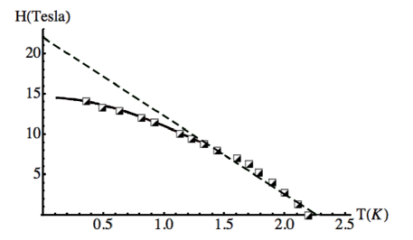
Figure 2: Temperature dependence of the upper critical magnetic field, $H^{x}_{c2}(T)$, numerically calculated from Eq.(15) al low enough temperatures, is shown by a solid line. The Ginzburg-Landau linear dependence (16), which is valid at $T_{c}-T\ll T_{c}$, is shown by broken line. Rectangles represent the experimental data [25].

To summarize, we have explained theoretically the observed destruction of superconductivity in the Q1D layered superconductor $\mathrm{Li_{0.9}Mo_{6}O_{17}}$ in a magnetic field parallel to its conducting axis [25], in the framework of triplet superconductivity scenario. We have also suggested the most probable triplet order parameter [see Eq.(9)]. It corresponds to the absence of Pauli paramagnetic destructive effects against superconductivity and is qualitatively consistent with a large value of the experimentally observed specific heat jump at the superconducting transition at $H=0$ [27].[Note that from the microscopic point of view, triplet phase can be stabilized in a Q1D superconductor as a result of repulsive interchain electron-electron interactions [39-41].]

Below, we would like to discuss the applicability of the Fermi liquid (FL) approach we have used in the Letter to describe the superconducting phase transition in the $\mathrm{Li_{0.9}Mo_{6}O_{17}}$. First of all, we note that at high enough temperatures, the Luttinger liquid effects are observed [42-44] in the $\mathrm{Li_{0.9}Mo_{6}O_{17}}$ conductor. This naturally reflects the Q1D nature of its electron spectrum (4),(5) and is not crucial for our analysis, since we consider the low temperature region, $T<T_{c}=2.2\ K$. In this context, it is important that from the theoretical point of view, the FL picture is restored at temperatures lower than $t_{z},t_{y}\simeq 10-45\ K$. Another point of concern is the experimentally observed increase of resistivity at $T\leq T_{min}\simeq 15-30\ K$. So far, its nature has not been clearly understood. At present, there exist two most popular competing points of view on this resistivity increase phenomenon: localization effects [45], and the possible partial charge-density-wave instability or the corresponding fluctuations [46,47]. Nevertheless, we stress that there are two experimental features [25], which are important for the validity of our analysis. The first one is based on the fact that the noted increase in resistivity is of the order of $\delta\rho/\rho\simeq 0.25$ [25] and, thus, small. The second feature is that the magnetoresistance at $T\simeq 4\ K$, as shown in Ref. [25], demonstrates quadratic behavior, $\delta\rho(H)/\rho(0)\sim H^{2}$, which is a direct test of the FL theory.

One of us (A.G.L.) is thankful to N.N. Bagmet and N.E. Hussey for useful discussions. This work was supported by the NSF under Grant No DMR-1104512.

^∗Also at: L.D. Landau Institute for Theoretical Physics, RAS, 2 Kosygina Street, Moscow 117334, Russia.

References

- (1) D. Jerome, A. Mazaud, M. Ribault, and K. Bechgaard, J. Phys. (Paris) Lett. 41, L95 (1980).
- (2) The Physics of Organic Superconductors and Conductors, edited by A.G. Lebed (Springer, Berlin, 2008).
- (3) M.-Y. Choi, P.M. Chaikin, S.Z. Huang et al., Phys. Rev. B 25, 6208 (1982).
- (4) S. Bouffard, M. Ribault, R. Brusseti et al., J. Phys. C 15, 2651 (1982).
- (5) M. Takigawa, H. Yasuoka, and G. Saito, J. Phys. Soc. Jpn. 56, 873 (1987).
- (6) A.A. Abrikosov, J. Low Temp. Phys. 53, 359 (1983).
- (7) A.G. Lebed, JETP Lett. 44, 114 (1986) [Pis’ma Zh. Eksp. Teor. Fiz. 44, 89 (1986)].
- (8) N. Dupuis, G. Montambaux, and C.A.R. Sa de Melo, Phys. Rev. Lett. 70, 2613 (1993).
- (9) I.J. Lee, M.J. Naughton, G.M. Danner, and P.M. Chaikin, Phys. Rev. Lett. 78, 3555 (1997).
- (10) A.G. Lebed, Phys. Rev. B 59, R721 (1999); A.G. Lebed, K. Machida, and M. Ozaki, Phys. Rev. B 62, R795 (2000).
- (11) A.I. Buzdin and V.V. Tugushev, Zh. Eksp. Teor. Phys. 85, 735 (1983) [Sov. Phys. JETP 58, 428 (1983)].
- (12) S. Yonezawa, S. Kusaba, Y. Maeno et al., Phys. Rev. Lett. 100, 117002 (2008).
- (13) A.G. Lebed and Si Wu, Phys. Rev. B 82, 172504 (2010).
- (14) M.D. Croitoru, M. Houzet, and A.I. Buzdin, Phys. Rev. Lett. 108, 207005 (2012).
- (15) A.G. Lebed, Phys. Rev. Lett. 107, 087004 (2011); Physica B 407, 1803 (2012); JETP Lett. 94, 382 (2011).
- (16) J. Shinagawa, Y. Kurosaki, F. Zhang et al., Phys. Rev. Lett. 98, 147002 (2007).
- (17) C. Bourbonnais and A. Sedeki, Phys. Rev. B 80, 085105 (2009).
- (18) I.J. Lee, S.E. Brown, W.G. Clark et al., Phys. Rev. Lett. 88, 017004 (2002).
- (19) I.J. Lee, P.M. Chaikin, and M.J. Naughton, Phys. Rev. B 62, R14669 (2000).
- (20) N. Belmechri, G. Abramovici and M. Heritier, Europhys. Lett. 82, 47009 (2008).
- (21) H. Tou, Y. Kitaoka, K. Ishida, K. Asayama, N. Kimura, Y. Onuki, E. Yamamoto, Y. Haga, and K. Maezawa, Phys. Rev. Lett. 80, 3129 (1998).
- (22) T.M. Rice and M. Sigrist, J. Phys.: Condens. Matter 7, L643 (1995).
- (23) A.P. Mackenzie and Y. Maeno, Rev. Mod. Phys. 75, 657 (2003).
- (24) K. Machida and T. Ohmi, Phys. Rev. Lett. 86, 850 (2001); K. Samokhin and M. Walker, Phys. Rev. B 66, 174501 (2002).
- (25) J.-F. Mercure, A.F. Bangura, Xiaofeng Xu, N. Wakeham, A. Carrington, P. Walmsley, M. Greenblatt, and N.E. Hussey, Phys. Rev. Lett., 108, 187003 (2012).
- (26) A.M. Clogston, Phys. Rev. Lett. 9, 266 (1962); B.S. Chandrasekhar, Appl. Phys. Lett. 1, 7 (1962).
- (27) See Supplemental Material for Ref.[25] at http://link.aps.org/supplemental/10.1103/PhysRevLett.108.187003 for details.
- (28) F. Zuo, J.S. Brooks, R.H. McKenzie, J.A. Schlueter, and J.M. Williams, Phys. Rev. B 61, 750 (2000).
- (29) A.A. Abrikosov, L.P. Gor’kov, and I.E. Dzyaloshinski, Methods of Quantum Field Theory in Statistical Physics (Dover, New York, 1975).
- (30) V.P. Mineev and K.V. Samokhin, Introduction to Unconventional Superconductivity (Gordon and Breach, Amsterdam, 1999).
- (31) M. Sigrist and K. Ueda, Rev. Mod. Phys. 63, 239 (1991).
- (32) A.G. Lebed and K. Yamaji, Phys. Rev. Lett. 80, 2697 (1998).
- (33) L.N. Bulaevskii, Sov. Phys. JETP, 38, 634 (1974).
- (34) R.A. Klemm, A. Luther, and M.R. Beasley, Phys. Rev. B 12, 877 (1975).
- (35) L.P. Gor’kov and D. Jerome, J. Phys. (Paris) Lett. 46, L643 (1985).
- (36) A.G. Lebed, JETP Lett. 94, 689 (2011).
- (37) L.P. Gor’kov, Zh. Eksp. Teor. Fiz. 37, 833 (1959) [Sov. Phys. JETP 10, 593 (1960)].
- (38) N.R. Werthamer, E. Helfand, and P.C. Hohenberg, Phys. Rev. 147, 295 (1966).
- (39) J.C. Nickel, R. Duprat, C. Bourbonnais, and N. Dupuis, Phys. Rev. Lett. 95, 247001 (2005).
- (40) K. Kuroki, R. Arita, and H. Aoki, Phys. Rev. B 63, 094509 (2001).
- (41) Y. Fuseya and Y. Suzumura, J. Phys. Soc. Jpn. 74, 1263 (2005).
- (42) F. Wang, J.V. Alvarez, S.-K. Mo, J.W. Allen, G.-H. Gweon, J. He, R. Jin, D. Mandrus, and H. Hochst, Phys. Rev. Lett. 96, 196403 (2006).
- (43) C.A.M. dos Santos, B.D. White, Yi-Kuo Yu, J.J. Neumeier, and J.A. Souza, Phys. Rev. Lett. 98, 266405 (2007).
- (44) N. Wakeham, A.F. Bangura, X. Xu, J.-F. Mercure, M. Greenblatt, and N.E. Hussey, Nature Commun. 2, 396 (2011).
- (45) M. Sato, Y. Matsuda, and H. Fukuyama, J. Phys. C: Solid State Phys. 20, L137 (1987).
- (46) X. Xu, A.F. Bangura, J.G. Analytis, J.D. Fletcher, M.M.J. French, N. Shannon, J. He, S. Zhang, D. Mandrus, R. Jin, and N.E. Hussey, Phys. Rev. Lett. 102, 206602 (2009).
- (47) Note that, in a quarter-filled Q1D conductor, a charge-density-wave phase can coexist with a spin-density-wave one, as shown in S. Mazumdar, S. Ramasesha, R.T. Clay, and D.K. Campbell, Phys. Rev. Lett. 82, 1522 (1999).