Quantum Communications Made Easy™
Deterministic Models of Bosonic Channels

Information theory establishes the ultimate limits on performance for noisy communication systems Shannon (1948). An accurate model of a physical communication device must include quantum effects, but typically including these makes the theory intractable. As a result communication capacities are not known, even for transmission between two users connected by an electromagnetic waveguide subject to gaussian noise. Here we present an exactly solvable model of communications with a fully quantum electromagnetic field. This allows us to find explicit expressions for all the point-to-point capacities of a noisy quantum channel, with implications for quantum key distribution, and fiber optical communications. We also develop a theory of quantum communication networks by solving some rudimentary quantum networks for broadcasting and multiple access. When possible, we compare the predictions of our new model with those of the orthodox quantum gaussian model and in all cases we find capacities in agreement to within a constant number of bits. Thus, in the limit of high signal to noise ratios our simple model captures the relevant physics of gaussian models while remaining amenable to detailed analysis.

I Introduction

A fundamental property of any communication system is the maximum rate of data transmission possible using the best communication schemes. This is called the capacity of a channel. It is usually calculated as a function of noise levels and subject to a limited power budget. In 1948, Shannon Shannon (1948) presented a beautiful theory of information both formulating and solving the capacity problem. For the specific case of a channel with additive white gaussian noise his formula can be solved explicitly giving the classical capacity $C$ as a function of the signal to noise ratio (SNR) as

$$C({\rm SNR})=\frac{1}{2}W\log(1+{\rm SNR}).$$ (1)

This formula guided the development of practical schemes that are now in use, culminating in efficient codes that come close to achieving the theoretical limit Richardson and Urbanke (2003).

Noise is not a purely mathematical abstraction, but must arise from some physical process. Such processes are properly described, of course, by quantum mechanics, and therefore calculating the true information carrying capacity of a channel requires a quantum-mechanical treatment. It is also natural, then, to consider new types of capacities, such as the capacity of a channel for transmitting quantum states coherently (the quantum capacity), or classical states securely (the private capacity). Unfortunately, unlike in classical information theory, for most quantum channels none of these capacities are known (see, for for example, Shor and Smolin (1996); DiVincenzo et al. (1998) for the quantum capacity and Hastings (2009) for the classical capacity, and Smith et al. (2008) for the private capacity).

Whereas much of the existing work on quantum channels has concentrated on abstract finite-dimensional channels, here we would like to study the problem in a more realistic setting. Our method is well suited to channels consisting of gaussian noise in bosonic electromagnetic modes, though it is substantially more general. We will be able to calculate classical, quantum, and private capacities for a wide range of realistic channels.

Because quantum information cannot be cloned Wootters and Zurek (1982), knowledge gained by the environment about a signal is necessarily detrimental to quantum transmission. This need to consider what information is transmitted to the environment as well as what goes to the intended receiver puts an analysis of quantum capacity on par with the study of the classical multi-user broadcast channel (which is also notoriously difficult to analyze Cover (1998)). To make the problem tractable we, following the work of Avestimehr et al. (2007), substitute a discretized and deterministic model for the actual channel. In the limit of high SNR this model will capture the important features of the real channel, and allow us to calculate capacities to within a small number of bits. The general approach can be thought of as discretizing the continuous system under consideration in a very simple way and then truncating signals smaller than the noise power. The result is a deterministic channel model that is easy to analyze.

II Additive Gaussian Channels

States of electromagnetic modes are described by their quadratures $P,Q$ and are called gaussian when they can be completely characterized by a matrix $\gamma$ containing the covariances of these quadratures Eisert and Wolf (2007). Such states can be visualized by their Wigner functions—quasi-probability distributions depicting the state’s location in phase space. Gaussian states have Wigner functions which are ellipsoids with gaussian profiles. Fig. 1(a) shows the Wigner function for a gaussian state with covariances $\sigma_{P},\sigma_{Q}$. The minimum uncertainty state has $\sigma_{P}\sigma_{Q}=1/2$ (in units of $\hbar$). Such states are always pure. Mixed states have $\sigma_{P}\sigma_{Q}>1/2$ and can be thought of as mixtures of pure states.

We will replace the quadratures $P,Q$ with a simpler discretized model described in Fig. 1(b). We call this the discrete quadrature (DQ) model. Roughly speaking, states in phase space are more distinguishable when their Wigner functions are less overlapping. To reflect this property, we divide phase space up into a lattice of nonoverlapping rectangles that we take to be perfectly distinguishable. The smallest physical state has area $1/2$. The Wigner function is thus replaced with several rectangles of area $1/2$ which tile the region of phase space where it is nonnegligable. The associated state in our model is a uniform mixture of these distinguishable rectangles.

The model of the action of a channel model will also be discrete: Since all the output states are perfectly distinguishable rectangles, every pair of input states will either be mapped to distinguishable outputs, or to the same output. Calculating the achieved communication rate is then a simple matter of counting the distinguishable output states. A full calculation of the capacity will also include a maximization over modulation schemes, i.e. the set of input states employed. Note that not all modulation schemes are physical. The choice must obey the following constraints:

• $\frac{1}{2}(\sigma_{Q}^{2}+\sigma_{P}^{2})\leq W$ (finite power)

• $\Delta P\Delta Q\geq 1/2$ (quantum uncertainty)

• $\Delta P\leq\sigma_{P},$ $\Delta Q\leq\sigma_{Q}$ (common sense)

(a)

(b)

Figure 1: Phase-space representation of states (Wigner Functions): (a) Wigner function of a gaussian mixed state with variances $\sigma_{Q}$ and $\sigma_{P}$. (b) The discrete quadrature model. The mixed state has been approximately decomposed into nonoverlapping rectangles with width $\Delta Q$ and height $\Delta P$. These rectangles are the discrete states of the model which replaces original physical system. We imagine them as approximations to the pure squeezed state shown at point $A$.

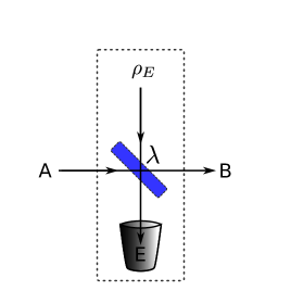
Figure 2: Additive gaussian noise noise channel. An input state in beam A is combined with an environmental input $\rho_{E}$ on a beamsplitter with transmitivity $\lambda$. One output beam is discarded (remains available only to the environment) and the other is the channel output B. When the environment’s input $\rho_{E}$ is a vacuum state, this gives the attenuation channel. When $\rho_{E}$ is a thermal state, it is the thermal noise channel.

The evolution of bosonic states under the action of channels is described by the evolution of the system’s quadratures. For gaussian noise, which arises from quadratic Hamiltonian interaction with gaussian environment modes, the allowed evolutions take a particularly simple form, being completely described by a symplectic matrix Holevo and Werner (2001). For example, $P\rightarrow\sqrt{\lambda}P+\sqrt{1-\lambda}\ r,\ Q\rightarrow\sqrt{\lambda}Q+\sqrt{1-\lambda}\ s$, results from interaction with an environment mode described by $r,s$ (see Fig. 2). The additive gaussian noise channel arises when the environment begins in a gaussian state, and the thermal noise channel, when it is initially in a thermal state.

II.1 Classical Capacity

Figure 3: The DQ model of the action of a channel. (a) The input space is divided up into tiles of $\Delta Q\times\Delta P$. (b) Attenuation has shrunk the tiles to $\sqrt{\lambda}\Delta Q\times\sqrt{\lambda}\Delta P$. (c) Noise has redenered some tiles confusable, so the effective tile size is increased. (d) If any tiles are smaller than the smallest tile size allowed by uncertainty, the tiles are enlarged again.

II.1.1 General Additive Gaussian Noise

(a)

(b)

Figure 4: The classical capacity of the attenuation channel. (a) For $\lambda=1/2$, the actual capacity $g((W-1/2)/2)/\ln 2$ and the capacity calculated using the discrete quadrature model $\log W$. (b) The difference between the actual and discrete quadrature capacity as a function of both $\lambda$ and power. Note that the difference is never greater than 1.4 bits.

We now apply our discretization procedure to model classical communication over an additive gaussian noise channel. Fig. 3 illustrates the following analysis. We suppose that the input signal has some average power constraint $W\geq\frac{1}{2}(\sigma_{P}^{2}+\sigma_{Q}^{2})$. Furthermore, we fix a modulation scheme, to be optimized over later, which amounts to deciding the shape of the rectangles in the discretization shown in Fig. 1b. Given the variables $\sigma_{P},\sigma_{Q}$ and rectangle shape $\Delta P,\Delta Q$ with $\Delta P\Delta Q=1/2$, our input space has $\sigma_{P}\sigma_{Q}/(\Delta P\Delta Q)$ distinguishable states (Fig. 3a). We must now determine how many distinguishable outputs these get mapped to. Attenuation by $\lambda$ maps the entire input space to a $\sqrt{\lambda}\sigma_{P}\times\sqrt{\lambda}\sigma_{Q}$ rectangle of $\sqrt{\lambda}\Delta P\times\sqrt{\lambda}\Delta Q$ tiles (Fig. 3b). When a noise of typical size $\sqrt{1-\lambda}\sigma_{r}$ is added to the $P$ quadrature, tiles closer than this are taken to be confusable, and similarly for $Q$, which leads us to “meta”-tiles of dimension

$$\max(\sqrt{\lambda}\Delta P,\sqrt{1-\lambda}\sigma_{r})\times\max(\sqrt{\lambda}\Delta Q,\sqrt{1-\lambda}\sigma_{s})\ {\rm(Fig.\ \ref{actionfigure}c).}$$ (2)

If it happens that this rectangle’s area is less than $1/2$ the tiles in Fig. 3c are smaller than the minimum tile size allowed by uncertainty. We must then chose a tile shape, $\Delta N\times\Delta M$ with $\Delta N\Delta M=1/2$ satisfying uncertainty. We thus find a final tile dimension of $\Delta\tilde{P}\times\Delta\tilde{Q}$ with

$$\Delta\tilde{P} \equiv\max(\sqrt{\lambda}\Delta P,\sqrt{1-\lambda}\sigma_{r},\Delta N)$$ (3)

$$\Delta\tilde{Q} \equiv\max(\sqrt{\lambda}\Delta Q,\sqrt{1-\lambda}\sigma_{s},\Delta M)\ \ {\rm(Fig.\ \ref{actionfigure}d)}.$$ (4)

This gives a total number of distinguishable output states of $\lambda\sigma_{P}\sigma_{Q}/(\Delta\tilde{P}\Delta\tilde{Q})$ and a classical capacity $\mathbf{C}$ of

$$\mathbf{C}=\max\log\left(\frac{\lambda\sigma_{P}\sigma_{Q}}{\Delta\tilde{P}\Delta\tilde{Q}}\right)\$$ (5)

where the maximization is over all of the constrained variables: $\frac{1}{2}(\sigma_{P}^{2}+\sigma_{Q}^{2})\leq W,\ \Delta P\Delta Q\geq\frac{1}{2},\ \Delta P\leq\sigma_{P},\ \Delta Q\leq\sigma_{Q},\ \Delta N\Delta M\geq\frac{1}{2}$. We now evaluate the preceding formula for some important special cases.

II.1.2 Example: Attenuation

The attenuation channel is an additive channel with transmissivity $\lambda$ and pure environment in a vacuum state with $\sigma_{r}=\sigma_{t}=\frac{1}{\sqrt{2}}$. To good approximation, this channel describes the propagation of the signal through lossy optical fiber. Letting $\Delta P=\Delta Q=\frac{1}{\sqrt{2}}$ and $\Delta M=\Delta N=\frac{1}{\sqrt{2}}$, minimizes $\Delta\tilde{P}\Delta\tilde{Q}=\frac{1}{2}$ while satisfying the constraints. This leads to a capacity of $\log\lceil 2W\lambda\rceil$. For this channel, we actually know the classical capacity exactly Giovannetti et al. (2004). Indeed, the true capacity $g\left(\lambda(W-\frac{1}{2})\right)/\ln 2$, where $g(x)=(x+1)\ln(x+1)-x\ln x$, differs from our estimate by no more than 1.4 bits (see Fig. 4).

II.1.3 Example: Classical Noise

When a channel applies gaussian-distributed kicks in phase space, it is called a classical noise channel. This arises as a limiting case of the thermal noise channel shown in Fig. 2 with $\lambda\rightarrow 1$ and $\sigma_{r}=\sigma_{s}\rightarrow\infty$ while keeping $\sigma_{r}\sqrt{1-\lambda}=\mu$. We would like to evaluate Eq. (5) for this channel, where we have $\Delta\tilde{P}=\max(\Delta P,\mu)$ and $\Delta\tilde{Q}=\max(\Delta Q,\mu)$.

First we consider the case $\mu^{2}\geq 1/2$. First note that $\Delta\tilde{P}\Delta\tilde{Q}\geq\mu^{2}$. Choosing $\Delta P=\Delta Q=1/\sqrt{2}$ achieves this lower bound. Note also that $\max_{W\geq\frac{1}{2}(\sigma_{P}^{2}+\sigma_{Q}^{2})}\sigma_{P}\sigma_{Q}=W$ is achieved for $\sigma_{P}=\sigma_{Q}=\sqrt{W}$. Thus by choosing $\Delta P=\Delta Q=1/\sqrt{2}$ and $\sigma_{P}=\sigma_{Q}=\sqrt{W}$ we simultaneously maximize $\sigma_{P}\sigma_{Q}$ and minimize $\Delta\tilde{P}\Delta\tilde{Q}$ while satisfying all the constraints in Eq. (5). We thus find a capacity of $\log(W/\mu^{2})$. In a similar way, when $\mu^{2}<1/2$, $\Delta\tilde{P}\Delta\tilde{Q}$ is minimized by $\Delta P=\Delta Q=1/\sqrt{2}$ so that by the same argument the capacity is now $\log(2W)$. A lower bound for the capacity of the classical noise channel with noise power $\mu^{2}$ is $\left(g(W-1/2+\mu^{2})-g(\mu^{2})\right)/\ln 2$. This is achieved by classical displacements of vaccuum states. This bound is within 1.45 bits of the true capacity Koenig and Smith (2012) and agrees with the DQ model to within 1 bit for all $\mu^{2}$.

II.1.4 Example: Dephasing

Another interesting special case is the classical dephasing channel, which adds classical noise of power $\mu^{2}$ to the $Q$ quadrature while leaving $P$ untouched. Starting from the quantum channel $P\rightarrow\sqrt{\lambda}P+\sqrt{1-\lambda}r$ and $Q\rightarrow\sqrt{\lambda}Q+\sqrt{1-\lambda}s$, we take the limit $\lambda\rightarrow 1$ with $(1-\lambda)\sigma_{s}^{2}=\mu^{2}$, $(1-\lambda)\sigma_{r}^{2}\rightarrow 0$. So we have the channel $P\rightarrow P$ and $Q\rightarrow Q+\xi$ where $\xi$ is a classical guassian random variable with variance $\mu^{2}$.

The discrete quadrature model of this channel is considered in Fig. 5 , where we have obtained a capacity estimate of $\log 2W$, independent of noise level. The modulation scheme to achieve this involves highly squeezed signal states. By choosing states very narrow in $P$ and broad in $Q$, we can pack nearly all of the signal into the noiseless quadrature. Thus, for classical transmission, such a channel achieves rates just as high as in the noiseless channel, albeit with more difficult modulation. This prediction is borne out by computing the Holevo information on the suggested squeezed ensemble, which an gives achievable rate that differs from $\log 2W$ by no more than a bit Holevo et al. (1999); Holevo and Werner (2001).

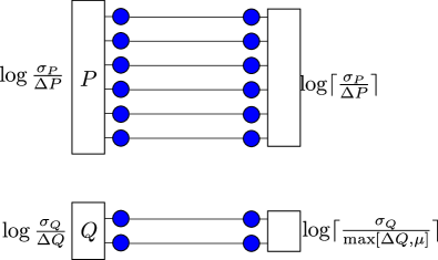
(a)

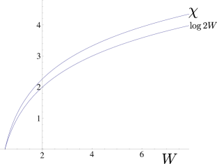
(b)

Figure 5: Dephasing channel. (a) Discrete quadrature model. The $\max[{\Delta Q,\mu}]$ in the denomiator of the $Q$ quadrature output takes into account that you cannot distinguish states smaller than either the size of the input or the size of the applied classical noise. The ‘ceiling’ brackets inside the logarithms avoid them blowing up if the noise is so high that there are fewer than one distinguishable states by this calculation. (b) Classical capacity of the dephasing channel with $\mu=1$. The capacity is achieved with $\Delta P=1/(2\sqrt{W})$ and $\Delta Q=\sqrt{W}$ and $\sigma_{P}=\sigma_{Q}=\sqrt{W}$. The squeezing and therefore the capacity is limited only by the input power. The lower line in the plot is the prediction from the discrete quadrature model, the upper is an exact calcuation of the Holevo quantity given a signal ensemble of maximally-squeezed pure states subject to the power constraint, which is an achievable rate $\chi=\left(g(\frac{2W\sqrt{1+\mu^{2}/(2W)}-1}{2})-g(\frac{\sqrt{1+\mu^{2}/(2W)}-1}{2})\right)/\ln 2$. Our model suggests this is not far from the actual capacity.

II.2 Quantum Capacity

As mentioned above, evaluating the quantum capacity $\mathbf{Q}$ requires assessing not only signals sent from sender to receiver, but also how information is leaked from sender to the channel’s environment. While this makes our calculations more complex, we will nevertheless find simple and reliable estimates for quantum capacities. The quantum capacity will be computed as the number of distinguishable states communcated to the channel’s output about which the environment knows nothing at all. This complete lack of knowledge enables one to communicate quantum superpositions of these distinguishable states, therefore our model imagines them to define the basis states of a Hilbert space that will be successfully transmitted. Note that this is exactly the definition of the private capacity Devetak (2005), and therefore our model will not be able to separate quantum and private capacities.

II.2.1 Example: Thermal Noise

We now turn our attention to the thermal noise channel, which maps $P\rightarrow\sqrt{\lambda}P+\sqrt{1-\lambda}\ r$ $Q\rightarrow\sqrt{\lambda}Q+\sqrt{1-\lambda}\ s$, where $r,s$ are the quadratures of a thermal state with average photon number $N_{E}$. Such a channel can be decomposed as a composition of a pure loss channel with an ideal amplifier as shown in Fig. 6a. This decomposition allows us to express the environment’s state as

$$\sqrt{1-\tilde{\lambda}}(P,Q)-\sqrt{\tilde{\lambda}}(r_{1},s_{1})$$ (6)

$$\sqrt{G}(r_{2},s_{2})+\sqrt{G-1}(P,-Q)$$ (7)

where $G=(1-\lambda)N_{E}+1$ and $\tilde{\lambda}=\lambda/G$ and $r_{1},s_{1}$ and $r_{2},s_{2}$ are the quadratures of two independent vacuum states.

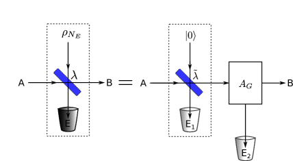
(a)

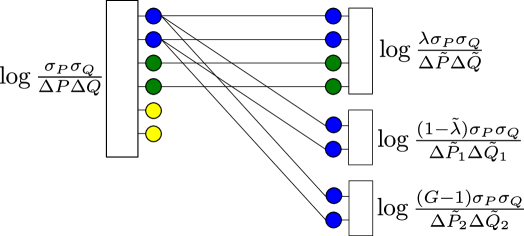
(b)

Figure 6: (a) Decomposition of thermal noise channel with average photon number $N_{E}$ into a pure attenuation channel with $\tilde{\lambda}=\lambda/G$ and a gain channel with gain $G$. (b) DQ model of this decomposition.

Following our prescription, an input with power $W$ and variances $\sigma_{P}^{2}+\sigma_{Q}^{2}\leq W$ we have $\lambda\sigma_{P}\sigma_{Q}/\Delta\tilde{P}\Delta\tilde{Q}$ distinguishable states at the output, or

$$S_{\textrm{output}}=\log(\lambda\sigma_{P}\sigma_{Q}/\Delta\tilde{P}\Delta\tilde{Q})$$ (8)

bits. The highest order bits of the input get mapped to $\log(\lambda\sigma_{P}\sigma_{Q}/\Delta\tilde{P}\Delta\tilde{Q})$ states at the output. Similarly, there are two environmental modes. Similarly, according to Eq. (6), the first environmental mode gets

$$S_{1}=\log\left((1-\tilde{\lambda})\sigma_{P}\sigma_{Q}/\Delta\tilde{P_{1}}\Delta\tilde{Q_{1}}\right)=\log\left(2(1-\lambda/G)\sigma_{P}\sigma_{Q}\right)$$ (9)

bits where $\Delta\tilde{P_{1}}=\max(\sqrt{1-\tilde{\lambda}}\Delta P,\Delta M_{1},\sqrt{\tilde{\lambda}}\sigma_{r_{1}})$ and $\Delta\tilde{Q_{1}}=\max(\sqrt{1-\tilde{\lambda}}\Delta Q,\Delta N_{1},\sqrt{\tilde{\lambda}}\sigma_{s_{1}})$. We always have $\Delta\tilde{P_{1}}\Delta\tilde{Q_{1}}\geq 1/2$, and $\Delta\tilde{P_{1}}\Delta\tilde{Q_{1}}=1/2$ can be achieved for appropriate $\Delta M_{1},\Delta N_{1}$.

For the second environmental mode, we have $S_{2}=\log\left((G-1)\sigma_{P}\sigma_{Q}/\Delta\tilde{P_{2}}\Delta\tilde{Q_{2}}\right)=\log\left(2(G-1)\sigma_{P}\sigma_{Q}/G\right)$ where $\Delta\tilde{P_{2}}=\max(\sqrt{G-1}\Delta P,\Delta M_{2},\sqrt{G}\sigma_{r_{2}})$ and $\Delta\tilde{Q_{2}}=\max(\sqrt{G-1}\Delta Q,\Delta N_{2},\sqrt{G}\sigma_{s_{2}})$ and $\Delta\tilde{P_{2}}\Delta\tilde{Q_{2}}=G/2$ is achievable.

Note that the high-order bits transmitted to both mode 1 and mode 2 are identical, but mode 1 gets more of them so that the total number of bits leaked to the environment is $S_{1}$. The quantum capacity is therefore

$$S_{\textrm{output}}-S_{1} =\log(\lambda\sigma_{P}\sigma_{Q}/\Delta\tilde{P}\Delta\tilde{Q})-\log\left(2(1-\lambda/G)\sigma_{P}\sigma_{Q}\right)$$ (10)

$$=\log\lambda-\log(1-\lambda/G)-\log 2\Delta\tilde{P}\Delta\tilde{Q}$$ (11)

$$=\log\lambda-\log(1-\frac{\lambda}{(1-\lambda)N_{E}+1})-\log 2\Delta\tilde{P}\Delta\tilde{Q}$$ (12)

We now evaluate (12) for the attenuation channel ($N_{E}=0$): As we showed in our discussion of the classical capacity of the attenuation channel, by appropriate choices of $\Delta P,\Delta Q$ and $\Delta M,\Delta N$, we can achieve $\Delta\tilde{P}\Delta\tilde{Q}=1/2$. Then the capacity is $\log{\lambda}-\log{(1-\lambda)}$ for $\lambda\geq 1/2$ and unlimited input power. This is exactly the quantum capacity of the gaussian attenuation channel Wolf et al. (2007). In fact our model offers slightly more information. Throughout in order for our model to make sense, the estimates of the number of levels transmitted must be integers. To ensure this in Eq. (10) we need to have power $W\gtrsim 1/\lambda$, which suggests the minimum power necessary to achieve capacity.

III Simultaneous Quantum and Classical Communication

Our model also allows for a simple understanding of the recently discovered Wilde et al. (2012) tradeoff between classical and quantum communication over the same optical channel. Switching between the two different optimal communication strategies for the two types of information (time sharing), gives a linear tradeoff between the two communication rates. In Wilde et al. (2012), it was shown that rate region for an attenuation channel could be substantially larger than this naive strategy would suggest. A glance at Figure 7 makes it clear that while sending quantum information at capacity, it is possible to simultaneously send some classical information with no degradation of the quantum transmission. Only after sending classical information at a rate greater than $\mathbf{C}-\mathbf{Q}$ does a linear tradeoff emerge.

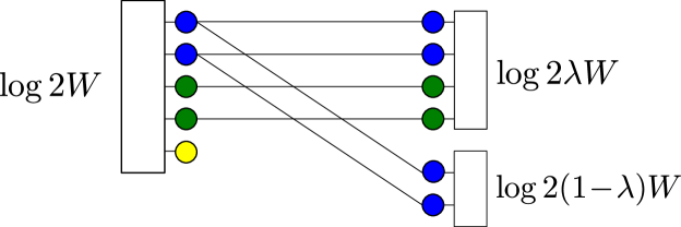
(a)

(b)

Figure 7: Simultaneous classical and quantum communication over a gaussian attenuation channel. (a) DQ Channel model. The higherst-order (blue) bits are seen by the environment and therefore can never be used for quantum communication. They can always be used for classical communication, even when the lower order bits are being used for quantum communication. (b) Rate region compared to the time-sharing tradeoff.

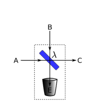
(a)

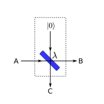
(b)

Figure 8: Multi-user Channels: (a) Multiple-access channel. (b) Broadcast channel.

IV Multi-User Communication

A useful and natural generalization of the channel capacity problem is when there are multiple senders and/or receivers. Our simple model is well adapted to extracting useful answers in this setting which is typically highly intractable, even in the classical setting Cover and Thomas (1991); El Gamal and Kim (2011). Below we consider two multi-user channels: The multiple access channel with two senders and one receiver and the broadcast channel with one sender and two receivers (see Fig. 8).

A simple multiple access channel is shown in Fig. 8a. Two senders $A$ and $B$ try to transmit information to a reciever $C$. The performance of such a channel is described by a rate region rather than a single capacity. The discrete quadrature model of this channel is shown in Fig. 9a and the predicted rate region is compared to existing bounds in Fig. 9b. Similarly, the DQ model and rate region for a simple broadcast channel, where one sender, $A$, tries to send information to two receivers $B$ and $C$, is shown in Fig. 10.

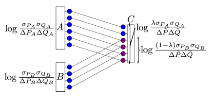
(a)

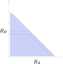
(b)

Figure 9: Simple multiple access channel. (a) Discrete quadrature model for the multiple access channel from Fig 8a with $\lambda W_{A}\geq(1-\lambda)W_{B}$. Discretizing the input quadratures as usual gives $\log\sigma_{P_{A}}\sigma_{Q_{A}}/\Delta P_{A}\Delta Q_{A}$ for sender $A$ and $\log\sigma_{P_{B}}\sigma_{Q_{B}}/\Delta P_{B}\Delta Q_{B}$ for sender $B$. The channel maps input quadratures $P_{A},Q_{A}$ and $P_{B},Q_{B}$ to outputs $\sqrt{\lambda}P_{A},Q_{A}+\sqrt{1-\lambda}P_{B},Q_{B}$. The highest order bits from $A$ remain distinguishable at the output regardless of what $B$ sends. The lower order bits are confusable; one of the senders can get information through to $C$ reliably so long as the other sender holds the corresponding bits fixed. (b) The classical-capacity rate region for the multiple access channel. The outer blue region is the upper bound from Yen and Shapiro (2005). The black lines indicate their achievable rate region with coherent states and the achievable region for our model with $\Delta P_{A}=\Delta Q_{A}$, $\Delta P_{B}=\Delta Q_{B}$. Our region is lower by just a fraction of a bit.

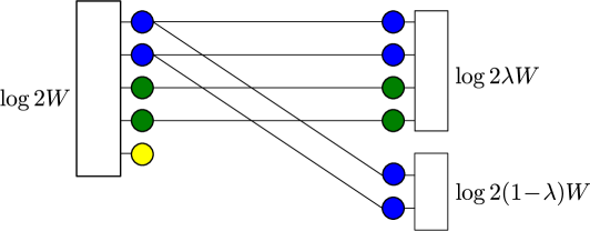
(a)

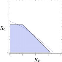
(b)

Figure 10: Broadcast channel. (a) The discrete quadrature model for the broadcast channel of 8b. We have taken $\Delta P=\Delta Q=1/\sqrt{2}$ which achieves optimality. The rate region is then given by $R_{c}\leq\log{2(1-\lambda)W}$ and $R_{B}+R_{C}\leq\log{2\lambda W}$. (b) The rate region is plotted for $W=50.5$, $\lambda=.8$ and compared to the lower bound from Guha et al. (2007) which they conjecture to be the actual capacity.

V Discussion

Our approach allows us to solve a number of vexing questions that are intractable in the orthodox model. For example, we can exactly solve models for single-user communication with thermal noise, as well as multi-user networks including broadcast and multiple-access channels. Perhaps, though, our model is too crude to capture the relevant behavior of quantum communication systems. We argue, to the contrary, that we capture the relevant physics by comparing the few solvable gaussian examples to our predictions where we find good agreement to within one or two bits. Furthermore, for examples where only lower bounds are available, we find good agreement with these, thus predicting that typically known lower bounds are equal, or at least close, to the ultimate capacities.

Our model also explains some previously known but counter-intuitive facts, rendering them almost obvious. For instance, we can explain why while classical capacity rises without bound as power increases, the quantum capacity saturates: Increasing power enhances transmission to both receiver and eavesdropper in equal measure. Put simply, if you’re trying to transmit privately, shouting your secrets doesn’t help. We have explained the results of Wilde et al. (2012), that time-sharing is not optimal for the classical-quantum tradeoff when trying to simultaneously transmit some of each type of information.

Finally, we can make some predictions. Within our deterministic model, entanglement between channel uses and other quantum tricks don’t appear to be useful. In particular, (1) Privacy and coherence are equivalent in our model. Therefore we predict the private and quantum capacities will always be nearly equal in gaussian channels, even though they can be very different in general Horodecki et al. (2005). (2) Two-way communication doesn’t help much for gaussian channels, again counter to the general case Bennett et al. (1996). (3) Gaussian channels have a single-letter capacity forumla to within a small number of bits (compare to Smith and Yard (2008); Smith and Smolin (2009)). (4) Capacities of gaussian channels are nearly additive (unlike the extreme superadditivity in Smith and Yard (2008); Smith and Smolin (2009)).

The “nearly” can, however, obscure some interesting effects. We know, for example, that gaussian channels can display superactivation, that is there exist pairs of gaussian channels each with zero capacity that can neverthelesss be used together to achieve positive capacity Smith et al. (2011). The resolution is that the resulting capacities are very small (the rate achieved with the joint channel in Smith et al. (2011) is only 0.06 bits). Our predictions are only meant to be with a few bits of the “correct” value so there is no contradiction, and our results should be asymptotically correct at high SNR.

References

- Shannon (1948) C. E. Shannon, Bell Syst. Tech. J. 27, 379 (1948).
- Richardson and Urbanke (2003) T. Richardson and R. Urbanke, IEEE Communications Magazine 41, 126 (2003).
- Shor and Smolin (1996) P. W. Shor and J. A. Smolin (1996), arXiv:quant-ph/9604006.
- DiVincenzo et al. (1998) D. DiVincenzo, P. W. Shor, and J. A. Smolin, Phys. Rev. A 57, 830 (1998), arXiv:quant-ph/9706061.
- Hastings (2009) M. Hastings, Nature Physics 5, 255 (2009).
- Smith et al. (2008) G. Smith, J. M. Renes, and J. A. Smolin, Phys. Rev. Lett. 100, 170502 (2008).
- Wootters and Zurek (1982) W. K. Wootters and W. H. Zurek, Nature 299, 802 (1982).
- Cover (1998) T. Cover, Information Theory, IEEE Transactions on 44, 2524 (1998), ISSN 0018-9448.
- Avestimehr et al. (2007) S. Avestimehr, S. Diggavi, and D. Tse, Allerton Conference on Communication, Control, and Computing (2007).
- Eisert and Wolf (2007) J. Eisert and M. M. Wolf, in Quantum Information with Continous Variables of Atoms and Light (Imperial College Press, London, 2007), pp. 23–42, arXiv:quant-ph/0505151.
- Holevo and Werner (2001) A. S. Holevo and R. F. Werner, Phys. Rev. A 63, 032312 (2001).
- Giovannetti et al. (2004) V. Giovannetti, S. Guha, S. Lloyd, L. Maccone, J. H. Shapiro, and H. P. Yuen, Phys. Rev. Lett. 92, 027902 (2004), URL http://link.aps.org/doi/10.1103/PhysRevLett.92.027902.
- Koenig and Smith (2012) R. Koenig and G. Smith (2012), arXiv:1207.0256.
- Holevo et al. (1999) A. S. Holevo, M. Sohma, and O. Hirota, Phys. Rev. A 59, 1820 (1999).
- Devetak (2005) I. Devetak, IEEE Trans. Inf. Theory 51, 44 (2005), arXiv:quant-ph/0304127.
- Wolf et al. (2007) M. M. Wolf, D. Perez-Garcia, and G. Giedke, Phys. Rev. Lett. 98, 130501 (2007), URL http://link.aps.org/doi/10.1103/PhysRevLett.98.130501.
- Wilde et al. (2012) M. M. Wilde, P. Hayden, and S. Guha, Phys. Rev. Lett. 108, 140501 (2012), URL http://link.aps.org/doi/10.1103/PhysRevLett.108.140501.
- Cover and Thomas (1991) T. M. Cover and J. A. Thomas, Elements of Information Theory (Wiley & Sons, 1991).
- El Gamal and Kim (2011) A. El Gamal and Y.-H. Kim, Network information theory (Cambridge University press, Cambridge, New York, Melbourne, 2011), ISBN 978-1-107-00873-1, URL http://opac.inria.fr/record=b1133858.
- Yen and Shapiro (2005) B. J. Yen and J. H. Shapiro, Phys. Rev. A 72, 062312 (2005), URL http://link.aps.org/doi/10.1103/PhysRevA.72.062312.
- Guha et al. (2007) S. Guha, J. H. Shapiro, and B. I. Erkmen, Phys. Rev. A 76, 032303 (2007), URL http://link.aps.org/doi/10.1103/PhysRevA.76.032303.
- Horodecki et al. (2005) K. Horodecki, M. Horodecki, P. Horodecki, and J. Oppenheim, Phys. Rev. Lett. 94, 160502 (2005).
- Bennett et al. (1996) C. H. Bennett, D. P. DiVincenzo, J. A. Smolin, and W. K. Wootters, Phys. Rev. A. 54, 3824 (1996), arXiv:quant-ph/9604024.
- Smith and Yard (2008) G. Smith and J. Yard, Science 351, 1812 (2008).
- Smith and Smolin (2009) G. Smith and J. A. Smolin, Phys. Rev. Lett. 103, 120503 (2009), URL http://link.aps.org/doi/10.1103/PhysRevLett.103.120503.
- Smith et al. (2011) G. Smith, J. A. Smolin, and J. Yard, Nature Photonics 5, 624 (2011).