A perturbational study of the lifetime of a Holstein polaron in the presence of weak disorder

Abstract

Using the momentum average (MA) approximation, we find an analytical expression for the disorder-averaged Green’s function of a Holstein polaron in a three-dimensional simple cubic lattice with random on-site energies. The on-site disorder is assumed to be weak compared to the kinetic energy of the polaron, and is treated perturbationally. Within this scheme, the states at the bottom of the polaron band are found to have an infinite lifetime, signaling a failure of perturbation theory at these energies. The higher-energy polaron states have a finite lifetime. We study this lifetime and the disorder-induced energy shift of these eigenstates for various strengths of disorder and electron-phonon coupling. We compare our findings to the predictions of Fermi’s golden rule and the average T-matrix method, and find a significant quantitative discrepancy at strong electron-phonon coupling, where the polaron lifetime is much shorter than Fermi’s golden rule prediction. We attribute this to the renormalization of the on-site potential by the electron-phonon coupling.

I introduction

Studying the behavior of solid state systems under the simultaneous action of disorder and interactions is a significant challenge in condensed matter physics. Strong correlations in interacting systems often give rise to sharp quasiparticles. Scattering of such quasiparticles from weak disorder should just limit their lifetime. For strong disorder and no interactions, it is well understoodAnderson that constructive interference of the backscattered waves can localize single particles such that they lose their itinerancy. If interactions are turned on, there is no consensus about the effect of disorder on the quasiparticles of interacting systems.

For example, consider polarons, which are the focus of this work, and which are quasiparticles comprising a charge carrier plus a cloud of phonons describing the lattice distortions in the vicinity of the charge. If one views the polaron as a particle with a renormalized mass, large disorder should result in Anderson localization. However, phonon-assisted hopping of carriers between localized states is well established as a conduction process in lightly doped semiconductors.Miller This suggests that, for suitable electron-phonon couplings, polarons may still be itinerant in a disorder potential that would localize particles with the same effective mass. A possible explanation for this was offered recently in Refs. MonaEPL, and Hadi, , where the momentum average (MA) approximation was used to show that the electron-phonon coupling renormalizes the disorder potential in a strongly energy-dependent manner, so that the effective disorder seen by polarons can be drastically different from the bare disorder.

References MonaEPL, and Hadi, focused on the effect of a single impurity potential on the polaron, although, as explained there, MA generalizes straightforwardly to other types of on-site potentials, including disordered ones. As such, it could be used to study numerically the effect of disorder, by generating results for various disorder realizations and analyzing their statistics. Such results have already been obtained for the HolsteinHolstein polaron using the statistical dynamic mean-field theory (sDMFT).F1 ; F2 Given the quite different underlying approximations, it might be useful to check whether MA leads to similar results.

A different approach, valid for weak disorder, is to use perturbation theory and perform the disorder average analytically, similarly to the Born approximation widely employed for charge carriers in the absence of electron-phonon coupling.ADM Because localization cannot be described within a perturbational calculation, the polaron eigenstates remain extended and self-averaging over all disorder realizations is appropriate.

Here we follow the latter approach and calculate, using MA and for weak disorder, the disorder-averaged Green’s function of the Holstein polaron and the resulting polaron lifetime and energy shift. MA is an accurate analytical method originally developed for calculating the Green’s function of Holstein polaron in clean systems,MA0 and later extended to other types of coupling.glen ; dominic MA is nonperturbative in the electron-phonon coupling as it sums all diagrams in the self-energy expansion, up to exponentially small terms that are neglected. It also has a variational interpretation, in terms of the allowed structure of the polaron cloud.B ; MAh MA can also be systematically improved by increasing this variational space,MAh giving rise to the MA⁽⁰⁾, MA⁽¹⁾, etc., flavors which become more accurate but at an increased computational cost. Because here we focus only on the lowest-energy polaron states, which are already accurately described at the MA⁽⁰⁾ level, in the following we restrict ourselves to this flavor and call it MA for simplicity.

The paper is organized as follows. In Sec. II, we present the generalization of MA to include disorder perturbationally. Sec. III contains the results and their analysis, and Sect. IV has our conclusions. Various computational details are organized and presented in several appendixes.

II The model and its solution

The Hamiltonian for a single Holstein polaron in a lattice with random on-site energies is

$${\cal H}={\cal H}_{\mathrm{d}}+{\hat{V}}_{\mathrm{el-ph}}={\cal H}_{0}+{\hat{V}}_{\mathrm{d}}+{\hat{V}}_{\mathrm{el-ph}},$$ (1)

where the non-interacting part of the Hamiltonian, ${\cal H}_{\mathrm{d}}$, is divided into $\hat{V}_{\mathrm{d}}=\sum_{i}\epsilon_{i}{c^{\dagger}_{i}}c_{i}$, describing the on-site disorder potential experienced by the charge carrier, and

$${\cal H}_{0}=-t\sum_{\langle i,j\rangle}(c^{\dagger}_{i}c_{j}+H.c.)+\Omega\sum_{i}{b^{\dagger}_{i}}b_{i},$$ (2)

describing the kinetic energy of charge carrier plus the (optical) phonon energies ($\hbar=1$). The interaction part

$$\hat{V}_{\mathrm{el-ph}}=g\sum_{i}{c^{\dagger}_{i}}c_{i}(b^{\dagger}_{i}+b_{i})$$ (3)

describes the Holstein coupling between the charge carrier and phonons. As usual, $c_{i}$ and $b_{i}$ are annihilation operators for carrier and phonon, respectively, on the simple cubic lattice of lattice constant $a$, whose sites are indexed by $i$. The spin of the carrier is a trivial degree of freedom in this model, and we ignore it. Throughout this work we limit ourselves to the single polaron limit, i.e. there is a single charge carrier in the system.

The on-site energies, $\{\epsilon_{i}\}$, are taken from an uncorrelated symmetric random distribution

$${\cal P}(\{\epsilon_{i}\})=\Pi_{i}{\cal P}(\epsilon_{i}).$$ (4)

For Anderson-type disorder ${\cal P}(\epsilon_{i})$ has the customary form:

$${\cal P}(\epsilon_{i})=\begin{cases}1/(2\Delta)&\text{if }-\Delta\leq\epsilon_{i}\leq\Delta\\ 0&\text{otherwise,}\end{cases}$$ (5)

while ${\cal P}(\epsilon_{i})=x\delta(\epsilon_{i}-\epsilon_{\mathrm{A}})+(1-x)\delta(\epsilon_{i}-\epsilon_{\mathrm{B}})$ for a binary alloy, with $x$ being the concentration of A-type atoms and energies shifted so that $x\epsilon_{A}+(1-x)\epsilon_{B}=0$.

Our aim is to calculate the Green’s function of this Holstein polaron and average it analytically over all disorder configurations given by Eq. (4). From now on, we use an overbar to denote disorder-averaged quantities. The strength of disorder, $\sigma\equiv\sqrt{\bar{\epsilon_{i}^{2}}}$, is taken to be weak compared to polaron bandwidth in the clean system, so that it can be treated perturbationally. As a result, the polaronic picture remains valid but its lifetime is expected to become finite due to scattering from the disorder potential $\hat{V}_{\mathrm{d}}$. It is precisely this disorder-induced lifetime that interests us.

Since $\hat{V}_{\mathrm{d}}$ is weak compared to other terms in the Hamiltonian, we treat it as a perturbation. Dividing the Hamiltonian as ${\cal H}={\cal H}_{\mathrm{H}}+\hat{V}_{\mathrm{d}}$, where ${\cal H}_{\mathrm{H}}$ is the Hamiltonian of the Holstein polaron in the clean lattice, we use Dyson’s identity, $\hat{G}(\omega)=\hat{G}_{\mathrm{H}}(\omega)+\hat{G}(\omega)\hat{V}_{\mathrm{d}}\hat{G}_{\mathrm{H}}(\omega)$, to relate the resolvent $\hat{G}(\omega)$ of the system with disorder, to $\hat{G}_{\mathrm{H}}(\omega)$ of the clean system. To the second order in $\hat{V}_{\mathrm{d}}$, we find

$$\hat{G}(\omega) \approx \hat{G}_{\mathrm{H}}(\omega)+\hat{G}_{\mathrm{H}}(\omega)\hat{V}_{\mathrm{d}}\hat{G}_{\mathrm{H}}(\omega)$$

$$+\hat{G}_{\mathrm{H}}(\omega)\hat{V}_{\mathrm{d}}\hat{G}_{\mathrm{H}}(\omega)\hat{V}_{\mathrm{d}}\hat{G}_{\mathrm{H}}(\omega).$$

Because disorder breaks translational invariance, the eigenstates for any individual disorder realization are not labeled by the momentum ${\mathbf{k}}$. However, averaging over all disorder configurations restores the translational invariance and makes momentum a good quantum number again. As a result, $\overline{\langle 0|c_{\mathbf{k}}\hat{G}(\omega)c^{\dagger}_{\mathbf{k}^{\prime}}|0\rangle}=\delta_{{\mathbf{k}},{\mathbf{k}^{\prime}}}\bar{G}({\mathbf{k}},\omega)$ and we only need to calculate the diagonal matrix element:

$$\bar{G}({\mathbf{k}},\omega)=G_{\mathrm{H}}({\mathbf{k}},\omega)+\sum_{i}\bar{\epsilon_{i}}\langle 0|c_{\mathbf{k}}\hat{G}_{\mathrm{H}}(\omega)c^{\dagger}_{i}c_{i}\hat{G}_{\mathrm{H}}(\omega)c^{\dagger}_{\mathbf{k}}|0\rangle\\ +\sum_{i,j}\overline{\epsilon_{i}\epsilon_{j}}\langle 0|c_{\mathbf{k}}\hat{G}_{\mathrm{H}}(\omega)c^{\dagger}_{i}c_{i}\hat{G}_{\mathrm{H}}(\omega)c^{\dagger}_{j}c_{j}\hat{G}_{\mathrm{H}}(\omega)c^{\dagger}_{\mathbf{k}}|0\rangle.$$ (6)

Here, $G_{\mathrm{H}}({\mathbf{k}},\omega)=\langle 0|c_{\mathbf{k}}\hat{G}(\omega)c^{\dagger}_{\mathbf{k}}|0\rangle$ is the polaron Green’s function in the clean system. For completeness, its MA solution is briefly reviewed in Appendix A.

Since $\bar{\epsilon_{i}}=0$ for symmetric disorder, the first-order contribution vanishes (a finite average can be removed trivially by an overall shift of the energy). Because of uncorrelated disorder, $\overline{\epsilon_{i}\epsilon_{j}}=\bar{\epsilon_{i}^{2}}\delta_{i,j}\equiv\sigma^{2}\delta_{i,j}$, and the disorder-averaged Green’s function becomes

$$\bar{G}({\mathbf{k}},\omega)=G_{\mathrm{H}}({\mathbf{k}},\omega)\\ +\sigma^{2}\sum_{i}\langle 0|c_{\mathbf{k}}\hat{G}_{\mathrm{H}}(\omega)c^{\dagger}_{i}c_{i}\hat{G}_{\mathrm{H}}(\omega)c^{\dagger}_{i}c_{i}\hat{G}_{\mathrm{H}}(\omega)c^{\dagger}_{\mathbf{k}}|0\rangle.$$

The challenge is to use MA to calculate the matrix elements appearing in the second term to the same level of accuracy as $G_{\mathrm{H}}({\mathbf{k}},\omega)$.MAh

These matrix elements can be broken into products of generalized Green’s functions by inserting identity operators, $\mathcal{I}$, between the creation and annihilation operators. Since the MA flavor we use here is equivalent with assuming that the phonon cloud only extends over one site,MAh at this level of accuracy it suffices to truncate $\mathcal{I}\approx\sum_{l,n}(1/n!)b_{l}^{\dagger n}|0\rangle\langle 0|b_{l}^{n}$, i.e., to ignore states with phonons at two or more sites (such states can be added systematically in higher flavors of MA). This leads to:

$$\bar{G}({\mathbf{k}},\omega)=G_{\mathrm{H}}({\mathbf{k}},\omega)+\sigma^{2}\sum_{i,l,s,n,m}\langle 0|c_{\mathbf{k}}\hat{G}_{\mathrm{H}}(\omega)c^{\dagger}_{i}b_{l}^{\dagger n}|0\rangle\\ \times\langle 0|b_{l}^{n}c_{i}\hat{G}_{\mathrm{H}}(\omega)c^{\dagger}_{i}b_{s}^{\dagger m}|0\rangle\langle 0|b_{s}^{m}c_{i}\hat{G}_{\mathrm{H}}(\omega)c^{\dagger}_{\mathbf{k}}|0\rangle/(n!m!).$$ (7)

This expression involves two sets of generalized propagators, namely $\langle 0|c_{\mathbf{k}}\hat{G}_{\mathrm{H}}(\omega)c^{\dagger}_{i}b_{l}^{\dagger n}|0\rangle$ and $\langle 0|b_{l}^{n}c_{i}\hat{G}_{\mathrm{H}}(\omega)c^{\dagger}_{i}b_{s}^{\dagger m}|0\rangle$. We now evaluate them.

First, as detailed in Appendix B, to the level of accuracy of MA, for $n\geq 1$ the first propagator vanishes unless $i=l$. Therefore, we have to evaluate $F^{(n)}_{{\mathbf{k}}i}(\omega)\equiv\langle 0|c_{\mathbf{k}}\hat{G}_{\mathrm{H}}(\omega)c^{\dagger}_{i}b_{i}^{\dagger n}|0\rangle$ for $n\geq 1$. Note that $F^{(0)}_{{\mathbf{k}}i}(\omega)$ is already known: $F^{(0)}_{{\mathbf{k}}i}(\omega)=\langle 0|c_{\mathbf{k}}\hat{G}_{\mathrm{H}}(\omega)c^{\dagger}_{i}|0\rangle=G_{\mathrm{H}}({\mathbf{k}},\omega)\exp(-i{\mathbf{k}}\cdot{\mathbf{R}}_{i})/\sqrt{N}$, since momentum is a good quantum number in the clean system. Here, $N\rightarrow\infty$ is the number of sites in the system. The details of the calculation for $n\geq 1$, which is related to that of $G_{\mathrm{H}}({\mathbf{k}},\omega)$, are presented in Appendix B. The final result is:

$$F^{(n)}_{{\mathbf{k}}i}(\omega)=\Gamma_{n}(\omega)F^{(0)}_{{\mathbf{k}}i}(\omega),$$ (8)

where $\Gamma_{n}(\omega)$ are easy to calculate products of continued fractions, see Eq. (25).

Next, we calculate $W^{nm}(\omega)=\langle 0|b_{i}^{n}c_{i}\hat{G}_{\mathrm{H}}(\omega)c^{\dagger}_{i}b_{i}^{\dagger m}|0\rangle$ to the same level of accuracy. Note that because of the invariance to translations in the clean system, this quantity is independent of $i$. The detailed derivation of these functions is presented in Appendix C.

With these expressions in hand, the disorder averaged Green’s function is, to second order in $\sigma$:

$$\bar{G}({\mathbf{k}},\omega) \approx G_{\mathrm{H}}({\mathbf{k}},\omega)+\sigma^{2}\left[G_{\mathrm{H}}({\mathbf{k}},\omega)\right]^{2}\times$$ (9)

$$\sum_{n,m=0}^{\infty}\frac{\Gamma_{n}(\omega)W^{n,m}(\omega)\Gamma_{m}(\omega)}{n!m!}.$$

To the same order, this identifies the sum in the previous equation as the disorder self-energy,

$$\Sigma_{\mathrm{dis}}(\omega)=\sigma^{2}\sum_{n,m=0}^{\infty}\frac{\Gamma_{n}(\omega)W^{n,m}(\omega)\Gamma_{m}(\omega)}{n!m!}.$$ (10)

This is our main result. From a computational point of view, because the factorials in the denominator grow rapidly with increasing index, the infinite sums can be safely truncated at finite values for $n$ and $m$. Cutoffs of 20 proved sufficient for all cases we examined.

Using $G_{\mathrm{H}}({\mathbf{k}},\omega)=1/(\omega-\varepsilon_{\mathbf{k}}-\Sigma_{\mathrm{MA}}(\omega)+i\eta)$, see Appendix A, we can finally write

$$\bar{G}({\mathbf{k}},\omega)=\frac{1}{\omega-\varepsilon_{\mathbf{k}}-\Sigma_{\mathrm{tot}}(\omega)+i\eta},$$ (11)

where the total self-energy is $\Sigma_{\mathrm{tot}}(\omega)=\Sigma_{\mathrm{MA}}(\omega)+\Sigma_{\mathrm{dis}}(\omega)$. This implicit summation gives a more accurate expression for the disorder-averaged Green’s function than Eq. (9), with which it agrees to ${\cal O}(\sigma^{4})$.

III results

We are now prepared to study the effect of weak disorder on the polaron lifetime and energy shift. At this level of perturbation theory, disorder only enters through its standard deviation $\sigma$. In the following, we assume Anderson disorder of width $2\Delta$, for which $\sigma=\Delta/\sqrt{3}$. We will use either $\Delta$ or $\sigma$ to characterize the disorder, as convenient, but we emphasize that any other type of disorder that has the same $\sigma$ would lead to the same answer within this perturbational approximation. To characterize the electron-phonon coupling strength, it is convenient to use the effective coupling $\lambda=g^{2}/(6t\Omega)$.

Once the Green’s function is known, the energy broadening of a polaron state of momentum ${\mathbf{k}}$, which is inversely proportional to its lifetime, is the width of the low-energy peak in the spectral function, $A({\mathbf{k}},\omega)=-\frac{1}{\pi}\mathrm{Im}\bar{G}({\mathbf{k}},\omega)$. This broadening measures the rate at which the polaron leaves that momentum state due to scattering from the impurity potential $\hat{V}_{\mathrm{d}}$. In a clean system, the polaron states are infinitely long lived, therefore the low-energy spectral weight is a Dirac delta function (in fact, a Lorentzian of width $\eta\rightarrow 0$). Mathematically, this is a consequence of the fact that (in the absence of disorder) the polaron self-energy $\Sigma_{\mathrm{MA}}(\omega)$ has a vanishing imaginary part for all energies inside the polaron band.

Disorder-induced finite lifetime broadens the delta functions into Lorentzians. As a reference, we review first the case without electron-phonon coupling, $\lambda=0$. The only nonzero term in Eq. (10) corresponds to $m=n=0$, therefore

$$\Sigma_{\mathrm{dis}}(\omega)=\sigma^{2}W^{0,0}(\omega)=\sigma^{2}g_{0}(\omega),$$ (12)

where

$$g_{0}(\omega)=\frac{1}{N}\sum_{{\mathbf{k}}}\frac{1}{\omega-\varepsilon_{\mathbf{k}}+i\eta}$$ (13)

is the momentum-averaged free propagator.

The resulting spectral weight has a peak of width $\tau_{\mathbf{k}}^{-1}$ centred at energy $E_{\mathbf{k}}$, found from the pole condition

$$\omega-\varepsilon_{\mathbf{k}}-\Sigma_{\mathrm{dis}}(\omega)+i\eta=0,$$ (14)

where $\omega=E_{\mathbf{k}}-i\tau_{\mathbf{k}}^{-1}$ and $\eta\rightarrow 0^{+}$.

Because $\tau_{\mathbf{k}}^{-1}\sim\sigma^{2}$ is small for weak disorder, we approximate $\Sigma_{\mathrm{dis}}(\omega)\approx\Sigma_{\mathrm{dis}}(E_{\mathbf{k}})+{\cal O}(\sigma^{4})$. Using this in Eq. (14) gives $E_{\mathbf{k}}$ and $\tau_{\mathbf{k}}^{-1}$ as follows:note

$$\begin{array}[]{l}\displaystyle E_{\mathbf{k}}=\varepsilon_{\mathbf{k}}+\mathrm{Re}\Sigma_{\mathrm{dis}}(E_{\mathbf{k}})\\ \displaystyle\tau^{-1}_{\mathbf{k}}=-\mathrm{Im}\Sigma_{\mathrm{dis}}(E_{\mathbf{k}}).\end{array}$$ (15)

The first expression determines the energy shift compared to the electron energy in the clean system, $\varepsilon_{\mathbf{k}}$. Since $\mathrm{Re}g_{0}(\omega)$ is negative for $\omega<0$ and positive for $\omega>0$, this implies a widening of the energy band in the presence of disorder.

Using Eq. (12), the inverse lifetime becomes $\tau_{\mathbf{k}}^{-1}=-\sigma^{2}\mathrm{Im}g_{0}(E_{\mathbf{k}}).$ However, $\mathrm{Im}g_{0}(E_{\mathbf{k}})$ is proportional to the total density of states (DOS) for the clean system,

$$\mathrm{Im}g_{0}(E_{\mathbf{k}})=-\frac{\pi}{N}\sum_{{\mathbf{k}}^{\prime}}\delta(E_{\mathbf{k}}-\varepsilon_{{\mathbf{k}}^{\prime}})=-\pi\rho_{0}(E_{\mathbf{k}}),$$

so that:

$$\tau_{\mathbf{k}}^{-1}=\pi\sigma^{2}\rho_{0}(E_{\mathbf{k}})=\pi\sigma^{2}\rho_{0}(\varepsilon_{\mathbf{k}})+{\cal O}(\sigma^{4}).$$ (16)

The last equality is simply Fermi’s golden rule. Since the density of states vanishes outside the bandwidth of the clean system, this result predicts infinite lifetime for all states with $|E_{\mathbf{k}}|\geq 6t$, and finite lifetime for all states in between. We will return to this point below.

When the electron-phonon coupling is turned on the analysis is performed similarly, but now using the appropriate total self-energy. The results are discussed next.

We first consider weak electron-phonon coupling, $\lambda=0.5$. In Fig. 1(a) we plot the polaron inverse lifetime for states in the polaron band, for two different values of the disorder strength, $\Delta=0.2t$ and $0.4t$ (squares and circles, respectively). These values are extracted from Lorentzian fits of the lowest peak in $A({\mathbf{k}},\omega)$, using Eqs. (15). The broadening $\eta$ was decreased until $E_{\mathbf{k}}$ and $\tau_{\mathbf{k}}$ converged to values independent of it.

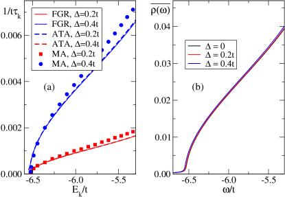
Figure 1: (Color online) (a) Inverse polaron lifetime $1/\tau_{\mathbf{k}}$ vs its peak energy $E_{\mathbf{k}}$, and (b) average DOS $\overline{\rho(\omega)}$ vs $\omega$, for a weak electron-phonon coupling and two values of the disorder $\Delta$. The solid and dashed lines are the corresponding Fermi golden rule (FGR) and ATA results, respectively (see text for more details). Other parameters are $\Omega=t,\eta/t=10^{-2}$ in (a) and $\eta/t=5\times 10^{-3}$ in (b).

For this small $\lambda$, the MA ground-state energy of the polaron in the clean system is $E_{P,GS}=-6.534t$. The weak disorder does not shift the eigenstates significantly. In fact, as shown in Fig. 1(b), the average density of states in the disordered system $\overline{\rho(\omega)}=-\frac{1}{\pi}\mathrm{Im}\sum_{\mathbf{k}}\bar{G}({\mathbf{k}},\omega)$ is nearly identical to that of the clean system, although the band becomes slightly broader with increasing $\Delta$. The inverse lifetime vanishes below the clean system bandedge, $E_{P,GS}$, and above it increases like $\sqrt{E_{\mathbf{k}}-E_{P,GS}}$, which is the expected clean system DOS at the bottom of the band. This is very similar to the $\lambda=0$ results, except for the renormalization of the DOS by the electron-phonon interactions. Indeed, if we think of the polaron as a simple quasiparticle whose density of states is $\rho(\omega)$ [renormalized from $\rho_{0}(\omega)$ for a free electron], the inverse lifetimes we find at the bottom of the polaron band are in good agreement with those predicted by Fermi’s golden rule (FGR), i.e., with $\pi\sigma^{2}\rho(E_{\mathbf{k}})$ (see full lines).

While the agreement between the two is good near the bottom of the band, it becomes systematically worse at higher energies. To verify that this amount of disorder is still sufficiently small so that the disagreement is not due to using perturbational results outside their validity range, we also show average T-matrix (ATA) results (dashed lines). ATA is a simple way to treat disorder beyond the lowest order in perturbation theory, for a system with $\lambda=0$. We briefly discuss it in Appendix D, as well as how we extended it to finite $\lambda$. ATA converges to $\pi\sigma^{2}\rho(\omega)$ in the limit of small $\sigma$, therefore the agreement between FGR and ATA confirms that the contribution of higher order terms in $\sigma$ is indeed negligible. The disagreement with MA at higher energies is, therefore, not an artifact of using perturbation theory.

The meaning of this disagreement at higher energies should, however, be treated with some caution. It is well knownB that this flavor of MA fails to reproduce the correct polaron+one phonon continuum, which should start at $E_{P,GS}+\Omega$ (this problem is fixed by MA⁽¹⁾ and higher flavors). One consequence is that MA overestimates the bandwidth of the polaron at weak couplings. Indeed, in Fig. 1(a) we see that the polaron band extends well past $E_{P,GS}+\Omega$. In other words, we know that at these higher energies MA is not accurate enough, so the results shown in Fig. 1 should only be trusted close to the bottom of the band, where the agreement is good.

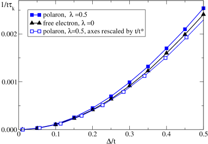
Figure 2: (Color online) Inverse lifetime of the polaron of momentum ${\mathbf{k}}=(\pi/8,0,0)$ and $\lambda=0.5$ vs the strength of disorder, $\Delta/t$ (full squares). The inverse lifetime for a free electron with the same momentum is shown by triangles. Empty squares show $1/(t^{*}\tau_{\mathbf{k}})$ vs $\Delta/t^{*}$ for the polaron (for this $\lambda$, $t^{*}=0.881t$). Other parameters are $\Omega=t,\eta/t=10^{-2}$.

The monotonic decrease of the polaron’s inverse lifetime with increasing disorder strength is shown in Fig. 2, for a polaron with momentum ${\mathbf{k}}=(\pi/8,0,0)$ and $\lambda=0.5$ (full squares). For comparison, also shown is the corresponding lifetime of a bare electron ($\lambda=0$, triangles) with the same momentum. Both curves show the expected $\propto\sigma^{2}$ increase predicted by Fermi’s golden rule, but the polaron lifetime is somewhat shorter. The most likely reason for this is the renormalization of the polaron mass by interactions. Indeed, if instead we plot $1/(t^{*}\tau_{\mathbf{k}})$ vs $\Delta/t^{*}$ for the polaron (empty squares), the results are much closer to those of the free electron, especially for small values of the disorder.

The conclusion, thus far, is that Fermi’s golden rule agrees well with our results at energies where this flavor of MA can be trusted. In other words, at weak electron-phonon coupling, the effect of disorder can be quantitatively understood if we think of the polaron as a simple particle with a renormalized mass (or DOS), and use Fermi’s golden rule.

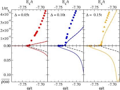
Figure 3: (Color online). Top panels: $1/(t\tau_{\mathbf{k}})$ vs $E_{\mathbf{k}}/t$ for three levels of disorder: $\Delta/t=0.05,0.1$ and $0.15$. The symbols shows the MA result for a strong coupling $\lambda=1.2$, while the full and dashed lines show Fermi’s golden rule and the ATA predictions, respectively. Bottom panels: The average DOS $\overline{\rho(\omega)}$ for that $\Delta$ (full line) and the DOS in the clean system, $\rho(\omega)$ (dashed line) vs $\omega$. Parameters are $\Omega=t,\eta=10^{-3}t$.

We now check whether this also holds true at strong electron-phonon coupling, for $\lambda=1.2$, where a robust small polaron appears in the clean system. The top panels in Fig. 3 show the polaron inverse lifetime vs. its energy for three levels of disorder (symbols), as well as the Fermi golden rule (full lines) and the ATA (dashed lines) predictions. The latter two are indistinguishable, confirming that these levels of disorder are indeed perturbationally small. The bottom panels show the average density of states in the corresponding disordered systems, $\overline{\rho(\omega)}$ (full lines). For comparison, the polaron DOS in the absence of disorder, $\rho(\omega)$, is also shown (dashed line).

Let us consider the DOS, first. As in the other cases, we see that with increasing disorder, the bandedge shifts down to lower energies. However, the effect is quantitatively much more significant here than at weaker couplings because the polaron band is much narrower. This is seen in Fig. 4, where we show the same densities of states but over the full polaron band. One surprise is that the entire polaron band moves to lower energies with increasing disorder. This is different from what happens for a simple particle, where the band broadens symmetrically on both sides. The different behavior at the upper edge is likely due to the difference in their spectra. While for a simple particle its band is the only feature in its spectrum, the spectrum of the polaron is quite complicated, with many other features, such as a band associated with the second bound state, the polaron+one-phonon continuum, etc., lying above the polaron band.MAh With increasing disorder all these features should move toward lower energies. Level repulsion from higher-energy states would explain why the upper edge of the polaron band moves to lower energies.

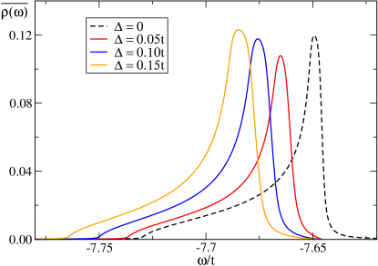
Figure 4: (Color online) The same average DOS vs $\omega$ displayed in the lower panels of Fig. 3, but now shown for the entire polaron band.

For the inverse lifetime we see that, as in the other cases, it vanishes for states with energy below the bandedge of the clean system, $E_{\bf k}<E_{P,GS}\approx-7.73t$. Because the shift of the disorder-averaged DOS is now significant, this means that, for a quite large energy range at the bottom of the band, the polaron has an infinite lifetime despite the presence of disorder. We emphasize that this is qualitatively similar to the result for a simple particle at the bottom of its band; the effect is simply quantitatively more pronounced here. The meaning of this (un-physical) infinite lifetime for these low-energy states is discussed in the conclusions; briefly, we believe that it signals a failure of the perturbation theory at these energies. These low-energy states are most susceptible to localization, so the perturbational calculation and its predictions are suspect here.

For higher-energy polaron states with $E_{\bf k}>E_{P,GS}$, the lifetime in the presence of disorder becomes finite, as expected. However, here the MA results disagrees quantitatively with the FGR and ATA results at all energies. The latter two are nearly indistinguishable, suggesting again that these levels of disorder are small enough that perturbation theory should be valid. The disagreement cannot be blamed on MA in this case; at such strong couplings and correspondingly low energies, MA is extremely accurate for the entire polaron band.MA0 ; MAh The disagreement is, therefore, meaningful.

Its origin can be quite easily traced. If we explicitly separate the $n=m=0$ contribution in the disorder self-energy, Eq. (10) becomes

$$\Sigma_{\rm dis}(\omega)=\sigma^{2}g_{0}(\omega-\Sigma_{\rm MA}(\omega))\\ +\sigma^{2}\sum_{n+m>0}\frac{\Gamma_{n}(\omega)W^{n,m}(\omega)\Gamma_{m}(\omega)}{n!m!}.$$ (17)

Figure 5: (i) FGR approximation for the disorder-averaged Green’s function of a carrier (double thin line), in terms of that of the free carrier (thin line) and uncorrelated disorder (dashed line) in the absence of electron-phonon coupling; (ii) FGR approximation for the disorder-averaged Green’s function of a polaron (double thick line), in terms of that of the clean polaron (thick line); (iii) clean polaron Green’s function in terms of free carrier (thin lines) and phonon (curly lines) propagators; (iv) the first few terms in the MA approximation for the disorder averaged Green’s function of a polaron.

If the contribution of the terms with $n+m>0$ can be ignored, this result leads to Fermi’s golden rule, since $\rho(\omega)=-{\frac{1}{\pi}}{\rm Im}g_{0}(\omega-\Sigma_{\rm MA}(\omega))$. The disagreement between MA and FGR, then, comes from the contribution of the terms with $n+m>0$. These terms cannot be ignored at strong electron-phonon coupling. Consider, for instance, $F_{{\bf k}i}^{(n)}(\omega)=\langle 0|c_{\bf k}\hat{G}_{\mathrm{H}}(\omega)c_{i}^{\dagger}b_{i}^{\dagger n}|0\rangle$, which is proportional to $\Gamma_{n}(\omega)$ and therefore is responsible for its appearance in $\Sigma_{\rm dis}(\omega)$. If we Fourier transform to real times, $F_{{\bf k}i}^{(n)}(\tau)$ is proportional to the amplitude of probability that if an electron is injected in the system at some moment, at a time $\tau$ later we find the electron in the presence of $n$ bosons, all at the same site. At strong couplings, the electron dresses itself with a large phonon cloud to become a polaron, so the probability of finding it with many phonons in its vicinity should be considerable, while the probability of finding the electron without any phonons $(n=0)$ is exponentially small. In the large $\lambda$ limit, the terms which are expected to contribute most are those with $n\approx g^{2}/\Omega^{2}$, i.e., values close to the average number of phonons in the polaron cloud. In contrast, for small $\lambda$ the phonon cloud is very fragile and, in fact, most of the time the electron is alone (resulting in a large quasiparticle weight). This is why, for weak coupling, keeping only the $n=m=0$ term in the sum provides a good approximation.

These considerations are illustrated diagramatically in Fig. 5. Panel (i) shows the Born approximation for the disorder averaged Green’s function of a carrier, which leads to Fermi golden’s rule expression for the lifetime, as already discussed. Panel (ii) shows its equivalent for the disorder averaged Green’s function of the polaron; as discussed above, this is equivalent with keeping only the $n=m=0$ term in the disorder self-energy, Eq. (10). Since each clean polaron propagator starts and ends with a free carrier propagator, this approximation means that the electron can scatter on disorder only in the absence of phonons; this is why this approximation fails at large electron-phonon coupling, where a large phonon cloud forms. In contrast, the full MA expression includes diagrams such as shown in panel (iv), where phonon and disorder lines cross. One can think of these as leading to an effective renormalization of the disorder strength, especially since these diagrams are very similar to those which result in the renormalization of a single impurity potential, discussed in Refs. MonaEPL, and Hadi, .

Our results in Fig. 3 reveal that this renormalization of the disorder (considerably) lowers the polaron lifetime. Thus, the strong electron-phonon coupling effectively enhances the strength of the disorder potential. Why this is so is not easy to infer from the results for a single impurity potential, where renormalization can either increase or decrease the bare potential, and even change its sign, and all these behaviors are seen at different energies (retardation effects are very significant). In any event, Fig. 3 shows that this renormalization is quantitatively significant.

A more detailed picture of the evolution of $\tau_{\bf k}$ and $E_{\bf k}$ with disorder $\Delta$ at strong coupling $\lambda$ is shown in Fig. 6 for two momenta ${\bf k}_{1}=(2\pi/9,0,0)$ and ${\bf k}_{2}=(\pi/6,0,0)$, which have free electron energies $\varepsilon_{{\bf k}_{1}}\approx-5.5t$ and $\varepsilon_{{\bf k}_{2}}\approx-5.7t$, respectively. In Fig. 6(a), we trace their inverse lifetimes as a function of disorder. At small $\Delta$ both these states are well above $E_{G,PS}$, and their scattering rates increase monotonically with $\Delta$, as one would expect on general grounds. However, the inverse lifetimes reach a maximum after which they begin to decrease fast and eventually vanish. The value of $\Delta$ where they vanish is the disorder at which that eigenstate has $E_{\mathbf{k}}=E_{P,GS}$. For larger disorder, this eigenstate moves below the free polaron bandedge, and its lifetime becomes infinite. This is more clearly shown by Fig. 6(b), where the inverse lifetimes are plotted vs. the corresponding eigenenergy $E_{\bf k}$ for these two momenta, as disorder is increased. This confirms that the scattering rates for both polaron states vanish when their energy drops below $E_{P,GS}$, whose location is marked by the asterisk. The value of $\Delta$ where this happens depends on how far above $E_{P,GS}$ was the energy $E_{\mathbf{k}}$ of this polaron, in the limit $\Delta\rightarrow 0$.

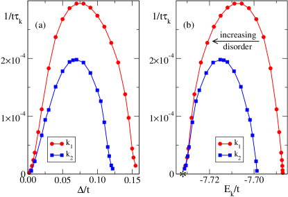
Figure 6: (Color online) (a) Inverse lifetime vs disorder, and (b) inverse lifetime vs energy $E_{\bf k}$, as disorder is turned on, for two momenta ${\bf k}_{1}=(2\pi/9,0,0)$ and ${\bf k}_{2}=(\pi/6,0,0)$, for a polaron with $\lambda=1.2,\Omega=t,\eta=10^{-3}t$. The asterisk in panel (b) marks the clean polaron GS energy in the clean system, $E_{P,GS}$, for these parameters. See text for more details.

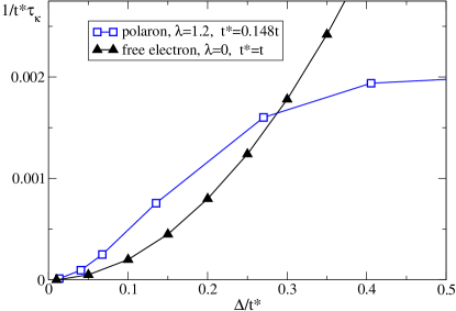
Figure 7: (color online) Same data as shown in Fig. 6(a) but with rescaled axes; $1/(t^{*}\tau_{\mathbf{k}})$ vs $\Delta/t^{*}$ for momentum ${\mathbf{k}}_{2}=(2\pi/9,0,0)$ (empty squares) is compared with the free electron lifetime (triangles) at the same momentum, for $\lambda=1.2$ where $t^{*}=0.148t$. Other parameters are $\Omega=t$ and $\eta/t=10^{-3}$.

Figure 3 showed that using the FGR estimate, i.e., $\tau_{\mathbf{k}}^{-1}=\pi\sigma^{2}\rho(E_{\bf k})$, is quantitatively wrong. We can also compare the polaron lifetime, where finite, with that of a free particle of renormalized mass, similar to the comparison in Fig. 2. This is shown in Fig. 7, where we compare $1/(t^{*}\tau_{\mathbf{k}})$ vs $\Delta/t^{*}$ for the polaron, with the inverse lifetime of a free electron with the same momentum. While roughly quadratic dependence is observed for the polaron at small disorder, the coefficient is quite different from that for the free electron. At higher disorder, the disagreement is even worse.

This shows that for intermediate and large electron-phonon coupling, where a heavy small polaron forms, its lifetime in the presence of disorder is not described quantitatively by the predictions corresponding to a simple particle with renormalized mass. The polaron has an internal structure which manifests itself in significant corrections to Fermi’s golden rule even for weak disorder. The scattering of the electron in the presence of its phonon cloud is quite different from that of a simple particle of the same effective mass, but without a cloud.MonaEPL ; Hadi

IV Summary and conclusions

Using MA to deal with the electron-phonon coupling and perturbation theory to deal with the weak disorder, we derived an expression for the disorder-averaged Green’s function of the Holstein polaron in a simple cubic lattice with random on-site energies. This allowed us to find an analytic expression for the lowest-order contribution from disorder to the polaron self-energy.

The disorder-averaged spectral weight was used to extract the lifetime and energy shift of various polaron states. For weak electron-phonon coupling, we found that the MA results are in reasonable quantitative agreement with those predicted by Fermi’s golden rule for a free particle with an appropriately renormalized mass.

At intermediate and larger electron-phonon coupling where a small polaron forms, however, the MA results quantitatively disagree with Fermi’s golden rule estimate everywhere the lifetime is finite and for all levels of disorder. The reason for this is the fact that the scattering of the electron in the presence of its (robust) phonon cloud is quite different from the scattering of a simple particle with renormalized mass. This is the same physics that leads to a significant renormalization of the disorder potential seen by a polaron as compared to the bare disorder.MonaEPL ; Hadi This demonstrates that, in the small polaron limit, it is wrong to assume that the only effect of the polaron cloud is to renormalize the polaron’s mass.

It is important to note that this calculation is only valid for weak disorder. It is based on perturbation theory, and in principle it can be improved by going to higher orders along the same lines we used to calculate the lowest-order contribution. However, one should remember that as disorder becomes stronger, Anderson localization will eventually occur, and that this cannot be captured within perturbation theory. Also, once disorder is large enough to lead to localization, the disorder-averaged Green’s function loses its meaning and usefulness. Instead, here the signature of localization becomes manifest in the distribution of various quantities such as the local density of states, not in their average value.

A surprise, at least at first sight, is the fact that this calculation predicts an infinite lifetime for a range of energies at the bottom of the polaron band. This interval can include a significant fraction of the polaron states, especially at stronger electron-phonon coupling and larger disorder. As we already mentioned, this is in fact similar to what happens for a free particle, which also is predicted, within this level of perturbation theory, to have an infinite lifetime for all momenta for which $|E_{\bf k}|>6t$. The difference is only quantitative: the energy shift for a free particle is tiny compared with its $12t$ bandwidth, whereas for a small polaron this shift can be comparable with its significantly narrower bandwidth even for rather weak disorder.

A likely reason for this can be inferred from the fact that, for a free particle, states at the band edge become localized immediately upon introduction of disorder. In other words, we already know that there is a finite range of energies (which, for weak disorder, falls outside the free particle bandwidth) where treating disorder perturbationally and calculating the disorder-averaged Green’s function is meaningless. It is then reasonable to conclude that the states for which this perturbational scheme predicts infinite lifetimes are, in fact, already localized. If this is correct and generalizes to the polaron case, it suggests that, unlike for a free particle, for a polaron localization sets in differently at the lower vs the upper polaron bandedge. We have already speculated that this difference may be due to the influence of the higher-energy states that exist in the polaron spectrum. Confirmation of these conclusions will require a study going beyond a perturbational treatment of disorder.

Appendix A MA solution for the clean system

Using the same notation as in the main part, the Holstein Hamiltonian for a clean system is

$${\cal H}_{\mathrm{H}}={\cal H}_{0}+\hat{V}_{\mathrm{el-ph}}.$$ (18)

To calculate $G_{\mathrm{H}}({\mathbf{k}},\omega)=\langle 0|c_{\mathbf{k}}\hat{G}_{\mathrm{H}}(\omega)c^{\dagger}_{\mathbf{k}}|0\rangle$, we use Dyson’s identity $\hat{G}_{\mathrm{H}}(\omega)=\hat{G}_{0}(\omega)+\hat{G}_{\mathrm{H}}(\omega)\hat{V}_{\mathrm{el-ph}}\hat{G}_{0}(\omega)$. The propagators for ${\cal H}_{0}$ are $\langle 0|c_{\mathbf{k}}b_{i}^{n}\hat{G}_{0}(\omega)c^{\dagger}_{\mathbf{k}^{\prime}}b_{j}^{\dagger m}|0\rangle=n!\delta_{n,m}\delta_{i,j}\delta_{\mathbf{k},\mathbf{k}^{\prime}}G_{0}({\mathbf{k}},\omega-n\Omega)$, where

$$G_{0}({\mathbf{k}},\omega)=\frac{1}{\omega-\varepsilon_{\bf k}+i\eta}.$$

We find

$$G_{\mathrm{H}}({\mathbf{k}},\omega)=G_{0}({\mathbf{k}},\omega)\left[1+g\sum_{i}{e^{i{\mathbf{k}}\cdot{\mathbf{R}}_{i}}\over\sqrt{N}}F^{(1)}_{\mathbf{k},i}(\omega)\right],$$ (19)

where we introduced the generalized propagators $F^{(n)}_{\mathbf{k},i}(\omega)=\langle 0|c_{\mathbf{k}}\hat{G}_{\mathrm{H}}(\omega)c_{i}^{\dagger}b^{\dagger n}_{i}|0\rangle$. Note that $F^{(0)}_{\mathbf{k},i}(\omega)=G_{\mathrm{H}}({\mathbf{k}},\omega)\exp(-i{\mathbf{k}}\cdot{\mathbf{R}}_{i})/\sqrt{N}$. Using the Dyson identity again, we find that for $n\geq 1$

$$F^{(n)}_{\mathbf{k},i}(\omega)=g\sum_{j\neq i}G_{0}(j,i,\omega-n\Omega)\langle 0|c_{\bf k}\hat{G}_{\mathrm{H}}(\omega)c_{j}^{\dagger}b_{j}^{\dagger}b_{i}^{\dagger n}|0\rangle\\ +gG_{0}(i,i,\omega-n\Omega)\left[nF^{(n-1)}_{\mathbf{k},i}(\omega)+F^{(n+1)}_{\mathbf{k},i}(\omega)\right].$$ (20)

Here

$$G_{0}(j,i,\omega)=\sum_{\mathbf{k}}{e^{i{\mathbf{k}}\cdot({\mathbf{R}}_{j}-{\mathbf{R}}_{i})}\over N}G_{0}({\mathbf{k}},\omega)$$

is the free propagator in real space (the sum is over the Brillouin zone). This propagator decays exponentially with the distance $|{\mathbf{R}}_{j}-{\mathbf{R}}_{i}|$ for energies outside the free particle continuum, $|\omega|>6t$. Since we are interested in energies $\omega-n\Omega\sim E_{P,GS}-n\Omega$, where the polaron GS energy $E_{P,GS}<-6t$, all these propagators become exponentially small for $j\neq i$. It is therefore a reasonable first approximation to ignore $j\neq i$ terms in the EOM written above. This is what the MA approximation does (higher flavors include $j\neq i$ terms in a certain progressionMAh ).

Within MA, then, we have for any $n\geq 1$

$$F^{(n)}_{\mathbf{k},i}(\omega)=gg_{0}(\omega-n\Omega)\left[nF^{(n-1)}_{\mathbf{k},i}(\omega)+F^{(n+1)}_{\mathbf{k},i}(\omega)\right],$$ (21)

where $g_{0}(\omega)=G_{0}(i,i,\omega)$; see Eq. (13). This recurrence relation is solved in terms of continued fractions:MA0

$$F^{(n)}_{\mathbf{k},i}(\omega)=A_{n}(\omega)F^{(n-1)}_{\mathbf{k},i}(\omega)$$ (22)

for any $n\geq 1$, where

$$A_{n}(\omega)=\frac{ngg_{0}(\omega-n\Omega)}{1-gg_{0}(\omega-n\Omega)A_{n+1}(\omega)}.$$ (23)

Finally, using $F^{(1)}_{\mathbf{k},i}(\omega)=A_{1}(\omega)F^{(0)}_{\mathbf{k},i}(\omega)$ in Eq. (19) leads to the MA solution:

$$G_{\mathrm{H}}({\mathbf{k}},\omega)={1\over\omega-\varepsilon_{\mathbf{k}}-\Sigma_{\mathrm{MA}}(\omega)+i\eta}$$

where

$$\Sigma_{\mathrm{MA}}(\omega)=gA_{1}(\omega).$$ (24)

Appendix B MA solution for $F_{{\mathbf{k}}i}^{(n)}(\omega)$

As discussed in the text, we need to calculate the propagators: $\langle 0|c_{\mathbf{k}}\hat{G}_{\mathrm{H}}(\omega)c^{\dagger}_{i}b^{\dagger n}_{s}|0\rangle$. Within the MA approximation (see above), this propagator is set to zero for all $i\neq s$, because it is proportional to $G_{0}(s,i,\omega-n\Omega)$. The only finite value is for $i=s$, in which case $\langle 0|c_{\mathbf{k}}\hat{G}_{\mathrm{H}}(\omega)c^{\dagger}_{i}b^{\dagger n}_{i}|0\rangle=F_{{\mathbf{k}}i}^{(n)}(\omega)$. These propagators have already been calculated above, $F^{(n)}_{\mathbf{k}i}(\omega)=A_{n}(\omega)F^{(n-1)}_{\mathbf{k}i}(\omega)=\dots=\Gamma_{n}(\omega)F^{(0)}_{\mathbf{k}i}(\omega)$, where

$$\Gamma_{n}(\omega)\equiv A_{n}(\omega)A_{n-1}(\omega)\cdots A_{1}(\omega).$$ (25)

Appendix C MA expression for $W^{n,m}(\omega)$

Here we calculate the remaining needed propagators, $W^{nm}(\omega)=\langle 0|b_{i}^{n}c_{i}\hat{G}_{\mathrm{H}}(\omega)c^{\dagger}_{i}b_{i}^{\dagger m}|0\rangle=W^{mn}(\omega)$. Because of this symmetry, we only need to find $W^{nm}(\omega)$ for $m\leq n$. Note that we already know $W^{00}(\omega)=\langle 0|c_{i}\hat{G}_{\mathrm{H}}(\omega)c^{\dagger}_{i}|0\rangle={1\over N}\sum_{{\mathbf{k}}}G_{\mathrm{H}}({\mathbf{k}},\omega)=g_{0}(\omega-\Sigma_{\mathrm{MA}}(\omega))$, and also $W^{n0}(\omega)=\langle 0|b_{i}^{n}c_{i}\hat{G}_{\mathrm{H}}(\omega)c^{\dagger}_{i}|0\rangle=\sum_{{\mathbf{k}}}{e^{-i{\mathbf{k}}\cdot{\mathbf{R}}_{i}}\over\sqrt{N}}\left[F_{{\mathbf{k}}i}^{(n)}(\omega)|_{\eta\rightarrow-\eta}\right]^{*}=\Gamma_{n}(\omega)g_{0}(\omega-\Sigma_{\mathrm{MA}}(\omega))$.

For any $m\geq 1$, writing the EOM for $W^{nm}(\omega)$ within the MA approximation (i.e., not allowing the electron to change its site), leads to

$$W^{n,m}(\omega) = m!g_{0}(\omega-m\Omega)\delta_{nm}+gg_{0}(\omega-m\Omega)$$ (26)

$$\times[mW^{n,m-1}(\omega)+W^{n,m+1}(\omega)].$$

For $m>n$, the delta function vanishes and Eq. (26) is identical to Eq. (21), hence

$$W^{n,m}(\omega)=A_{m}(\omega)W^{n,m-1}(\omega).$$ (27)

In particular, this gives $W^{n,n+1}(\omega)=A_{n+1}(\omega)W^{n,n}(\omega)$. Using this in Eq. (26) with $n=m$ relates $W^{n,n}(\omega)$ to $W^{n,n-1}(\omega)$:

$$W^{n,n}(\omega)=A_{n}(\omega)W^{n,n-1}(\omega)+\frac{(n-1)!}{g}A_{n}(\omega).$$ (28)

This is taken together with the EOM for $1\leq m\leq n-1$

$$W^{n,m}(\omega)=gg_{0}(\omega-m\Omega)\times[mW^{n,m-1}(\omega)+W^{n,m+1}(\omega)]$$

to give a system of $n$ equations with $n$ unknowns $W^{n,m}(\omega)$, $m=1,..,n$ [$W^{n,0}(\omega)$ is known; see above]. This can be solved in many ways, including direct numerical solution. A nicer approach is to use the linearity of this system of equations to split it into two different systems, one which has only $\frac{(n-1)!}{g}A_{n}(\omega)$ and one which has only $gg_{0}(\omega-\Omega)W^{n,0}(\omega)$ as inhomogeneous parts. These can be solved analytically, to give

$$W^{n,m}(\omega)=\Gamma_{m}(\omega)W^{n,0}(\omega)+\tilde{\Gamma}_{m}(\omega)\frac{(n-1)!A_{n}(\omega)}{g[1-A_{n}(\omega)B_{n}(\omega)]},$$

where $\tilde{\Gamma}_{m}(\omega)=B_{m+1}(\omega)B_{m+2}(\omega)\cdots B_{n}(\omega)$ for $m<n$ while $\tilde{\Gamma}_{n}(\omega)=1$, and

$$B_{m+1}(\omega)=\frac{gg_{0}(\omega-m\Omega)}{1-(m-1)gg_{0}(\omega-m\Omega)B_{m}(\omega)}$$

are continued fractions ending at $B_{2}(\omega)=gg_{0}(\omega-\Omega)$.

Appendix D ATA self-energy

ATAElliot ; book relates the disorder part of the self-energy of a single particle to the disorder average of its transfer matrix through a single impurity with on-site energy $\epsilon$:

$$\Sigma_{\mathrm{ATA}}(\omega)=\frac{\bar{t}}{1+\bar{t}g_{0}(\omega)},$$ (29)

where $t=\epsilon/(1-\epsilon g_{0}(\omega))$ is the sum over all single impurity scattering contributions. $g_{0}(\omega)$ is the momentum average of the free particle propagator, see Eq. (13).

For Anderson-type disorder we find

$$\bar{t} = \frac{1}{2\Delta}\int_{-\Delta}^{\Delta}\frac{\epsilon d\epsilon}{1-\epsilon g_{0}({\omega})}$$

$$= -\frac{1}{g_{0}({\omega})}+\frac{1}{2\Delta g_{0}^{2}({\omega})}\ln\frac{1+\Delta g_{0}({\omega})}{1-\Delta g_{0}({\omega})}.$$

Expanding to lowest order regains the perturbational result, Eq. (12): $\Sigma_{\mathrm{ATA}}(\omega)\approx\frac{\Delta^{2}}{3}g_{0}({\omega})=\sigma^{2}g_{0}({\omega})$. Differences between ATA and FGR show that disorder is so large that multiple scattering processes off the same impurity cannot be ignored anymore.

To extend ATA to the Holstein model, we note that difference between the MA clean polaron’s Green’s function and that of the free electron is the appearance of $\Sigma_{\mathrm{MA}}(\omega)$. This simply modifies $g_{0}(\omega)\rightarrow g_{0}(\omega-\Sigma_{\mathrm{MA}}(\omega))$ in all the above equations. As discussed above, this approximation implies that there is no crossing between phonon lines and scattering lines, in diagramatic terms. Our results show that this is a bad approximation at larger electron-phonon coupling.

References

- (1) P. W. Anderson, Phys. Rev. 109, 1492 (1958).
- (2) A. Miller and E. Abrahams, Phys. Rev. 120, 745 (1960).
- (3) M. Berciu, A. S. Mishchenko, and N. Nagaosa, Europhys. Lett. 89, 37007 (2010).
- (4) H. Ebrahimnejad and M. Berciu, Phys. Rev. B 85, 165117 (2012).
- (5) T. Holstein, Ann. Phys. (N.Y.) 8, 325 (1959); 8, 343 (1959).
- (6) F. X. Bronold and H. Fehske, Phys. Rev. B 66, 073102 (2002); F. X. Bronold, A. Alvermann, and H. Fehske, Philos. Mag. 84, 673 (2004). See also A. Alvermann and H. Fehske, Local Distribution Approach, Lecture Notes in Physics Vol. 739 (Springer, 2008), p. 505- 526.
- (7) S. Ciuchi, F. de Pasquale, S. Fratini, and D. Feinberg, Phys. Rev. B 56, 4494 (1997).
- (8) A. A. Abrikosov, L. P. Gorkov and I. Ye. Dzyaloshinski, Methods of quantum field theory in statistical physics (Dover, New York, 1975).
- (9) M. Berciu, Phys. Rev. Lett. 97, 036402 (2006); G. L. Goodvin, M. Berciu, and G. A. Sawatzky, Phys. Rev. B 74, 245104 (2006).
- (10) G. L. Goodvin and M. Berciu, Phys. Rev. B 78, 235120 (2008).
- (11) M. Berciu and H. Fehske, Phys. Rev. B 82, 085116 (2010); D. J. J. Marchand, G. De Filippis, V. Cataudella, M. Berciu, N. Nagaosa, N. V. Prokof’ev, A. S. Mishchenko, and P. C. E. Stamp, Phys. Rev. Lett. 105, 266605 (2010).
- (12) O . S. Barisic, Phys. Rev. Lett. 98, 209701 (2007); M. Berciu, Phys. Rev. Lett. 98, 209702 (2007).
- (13) M. Berciu and G. L. Goodvin, Phys. Rev. B 76, 165109 (2007) .
- (14) Strictly speaking, the lifetime is defined with an additional factor of 2.
- (15) E. N. Economou, Green’s Functions in Quantum Physics, 3rd edition (Springer-Verlag, New York, 2006), or A. Gonis, “Green Functions for Ordered and Disordered Systems” (Elsevier, Amsterdam, 1992).
- (16) R. J. Elliot, J. A. Krumhansl and P. L. Leath, Rev. Mod. Phys. 46, 465 (1974).