Skyrme pseudo-potential-based EDF parametrisation for spuriousity-free MR-EDF calculations

Abstract

First exploratory steps towards a pseudo-potential-based Skyrme energy density functional for spuriousity-free multi-reference calculations are presented. A qualitatively acceptable fit can be accomplished by adding simple three- and four-body contact terms to the standard central plus spin-orbit two-body terms. To achieve quantitative predictive power, higher-order terms, e.g. velocity-dependent three-body terms, will be required.

1 Introduction

Methods based on the use of effective energy density functionals (EDFs) [1] currently provide the only set of theoretical tools that can be applied to all bound atomic nuclei but the lightest ones in a systematic manner irrespective of their mass, isospin, and deformation. One underlying assumption is that of a universal effective energy functional that depends on normal and anomalous one-body density matrices and that re-sums the in-medium correlations whose details are irrelevant for low-energy nuclear structure physics. Nuclear EDF methods coexist on two distinct levels. On the first level, that is traditionally called self-consistent mean-field theory, Hartree-Fock (HF) or Hartree-Fock-Bogoliubov (HFB), a single product state provides the normal and anomalous density matrices that enter the EDF. We call this type of method a single-reference (SR) approach. Exploiting the concept of symmetry breaking as a consequence of the nuclear Jahn-Teller effect [2], collective correlations that correspond to multipole deformations or superfluidity can be easily modelled at the expense of losing good quantum numbers. On the second level, often called ”beyond-mean-field methods”, symmetry restoration and configuration mixing can be achieved within the Generator Coordinate Method (GCM) framework. Such method is referred to as a multi-reference (MR) approach [3]. The MR techniques aim at the explicit description of correlations that are related to the small finite size of the nucleus and that neither can be easily absorbed into the EDF, nor be described by a single SR state. Typical examples are the mixing of different shapes that coexist in a nucleus or the restoration of symmetries that are broken at the SR level. Besides describing correlated ground states, the MR approach also gives access to excited states and transition moments between them taking selection rules into account.

Multi-reference techniques based on energy density functionals rely on the extension of the EDF to non-diagonal energy kernels. The generalised Wick theorem [4] provides the formal framework when the EDF is defined as the expectation value of a genuine Hamilton operator. The energy functionals widely used in nuclear physics, however, are not of this form. We denote these as ”general functional” in what follows. The standard procedure for the MR extension of such general functionals is made by formal analogy with the Hamiltonian case, cf. [5, 6] and references therein. It has been pointed out a few years ago that the usual procedure to set up the non-diagonal kernels of a general EDF is ill-defined [5, 6, 7, 8, 9]. It gives rise to spurious contributions to the energy that can manifest themselves for example through divergences and/or finite steps when plotting the symmetry-restored energy as a function of a collective coordinate [5, 8]. It also makes MR calculations return non-zero energies when restoring negative particle numbers [8, 10]. These difficulties can be traced back to a breaking of the Pauli principle when setting up the EDF. In one way or the other, this is the case for all modern parametrisations of the nuclear EDF. It is motivated either by phenomenology or for computational reasons [1, 11].

One popular choice for a general nuclear EDF is historically based on two- and three-body contact pseudo-potentials proposed by Skyrme [12]. In the earliest adjustments of its coupling constants for nuclear EDF calculations it was used as a genuine Hamilton operator. This gave rise to three major problems in the resulting parametrisations: (i) the incompressibility $K_{\infty}$ of homogeneous symmetric infinite nuclear matter (INM) was unavoidably much larger than the empirical one; (ii) fits that constrain other INM properties such as isoscalar effective mass $m^{*}_{0}/m$, saturation density $\rho_{\text{sat}}$ and symmetry energy coefficient $a_{\text{sym}}$ to empirical values provided parametrisations that were unstable in the spin channel as indicated by the Landau parameter $g_{0}$ being smaller than $-1$ [13], and (iii) pairing matrix elements were far too small or even repulsive. Problem (ii) could be circumvented reinterpreting the contact three-body force $t_{3}\,\delta({\mathbf{r}}_{1}-{\mathbf{r}}_{2})\delta({\mathbf{r}}_{1}-{\mathbf{r}}_{3})$ as a density-dependent two-body force $\tfrac{1}{6}\,t_{3}\,(1+x_{3}\hat{P}^{\sigma}_{12})\,\rho_{0}^{\alpha}[({\mathbf{r}}_{1}+{\mathbf{r}}_{2})/2]\,\delta({\mathbf{r}}_{1}-{\mathbf{r}}_{2})$ with $\alpha=1$, where $\rho_{0}({\mathbf{r}})=\rho_{n}({\mathbf{r}})+\rho_{p}({\mathbf{r}})$ is the isoscalar density and $\hat{P}^{\sigma}_{12}$ the spin-exchange operator, respectively, which alters the so-called ”time-odd” part of the functional that governs the effective spin-spin interaction. Problem (i) could then be solved by reducing the exponent $\alpha$ from 1 to values between about $1/6$ and $1/3$. And for most parametrisations of the Skyrme EDF, problem (iii) was removed by using different vertices in the particle-hole and particle-particle channels that were independently adjusted to data. In addition, some specific terms in the EDF are often suppressed or approximated to simplify the numerical treatment [1]. In the past this has led to high-precision parametrisations of the Skyrme EDF that kept a relatively simple form [1, 14] and were numerically efficient, at the expense of sacrificing the exchange symmetry of the EDF. Other variants of the nuclear EDF have been set-up directly through their energy density without any reference to an underlying effective interaction [15, 16].

The breaking of the exchange symmetry that results from this practice introduces what is known as spurious ”self-interaction” in density functional theory for condensed matter [17]. An analysis of the same problem in the context of effective interactions as used in nuclear physics has been given in Ref. [18]. A similar spurious ”self-pairing” appears when the normal and pairing parts of the EDF are not derived from the same effective interaction as pointed out in Ref. [8]. According to Ref. [6], divergences and steps in MR EDF calculations originate from unphysical weights such self-interaction and self-pairing contributions are multiplied with. Based on this analysis, a regularisation scheme that modifies those ill-defined weights while keeping the self-interaction itself has been proposed in Ref. [6] and applied with success to the case of pure particle-number projection in Ref. [8].

Not all general functionals are regularizable, though. The formalism can be applied only to functionals that correspond to polynomials in the density matrices [6, 9]. Parametrisations of a general regularizable Skyrme-type EDF of minimal form have been constructed recently [11] and are currently used to test the regularised MR EDF scheme for general configuration mixing. Constraining the EDF to polynomial form makes its fit more difficult.

In parallel, we also started the construction of functionals that are free of spuriosities from the outset by setting them up as the expectation value of a genuine Skyrme-type Hamilton operator taking all exchange and pairing terms into account such that the Pauli principle is obeyed. By construction, this removes all spurious contributions to the EDF at the price of having less independent terms in the EDF. In what follows, we denote such functionals a ”pseudo-potential generated EDF”. This replaces the problem of how to set up a formalism for the extension of a general and flexible EDF to non-diagonal kernels for MR calculations by the problems of what is the most efficient form for a predictive pseudo potential that can be straightforwardly used in MR calculations and how to adjust it to data. This is a difficult task, as a pseudo-potential-based functional has much less independent coupling constants than a general functional of the same form. To be usable in SR and MR calculations incorporating pairing correlations, it is mandatory that the functional gives a reasonable description of the spin and pairing channels of the interaction. Otherwise the level sequence after angular-momentum projection is likely to be unrealistic. However, the difficulty to have even the correct sign of the interaction in these two channels has been among of the major motivations to abandon Skyrme-type pseudo-potential-based EDFs in favour of the general ones in the 1970s.

The aim of this contribution is to present the first explorative steps towards the construction of a predictive pseudo-potential based EDF. We present the adjustment of a parametrisation that achieves an acceptable qualitative description in all channels of the interaction by adding three- and four-body contact terms without gradients to a standard two-body Skyrme operator. It will serve to benchmark MR EDF calculations and as a reference for what can be achieved without introducing derivatives in the new terms.

2 Pseudo-potential-based EDF

The pseudo-Hamiltonian used in the present work takes the form

$$\hat{H}=\hat{T}^{(1)}+\hat{v}^{(2\text{Sk})}+\hat{v}^{(2\text{C})}+\hat{v}^{(3\text{Sk})}+\hat{v}^{(4\text{Sk})}\,,$$ (1)

where $\hat{T}^{(1)}$ is the kinetic energy operator and $\hat{v}^{(2\text{C})}$ the Coulomb interaction, which take their standard form. The $\hat{v}^{(N\text{Sk})}$ are the $N$-body parts of the Skyrme-type pseudo-potential for which we consider here the form

$$\hat{v}^{(2Sk)} ={t_{0}}\left(1+{x_{0}}\hat{P}^{\sigma}_{12}\right)\hat{\delta}_{r^{\,}_{1}r^{\,}_{2}}$$ (2a)

$$+\frac{{t_{1}}}{2}\left(1+{x_{1}}\hat{P}^{\sigma}_{12}\right)\left(\hat{{\mathbf{k}}}^{\,\prime\,2}_{12}\hat{\delta}_{r^{\,}_{1}r^{\,}_{2}}+\hat{\delta}_{r^{\,}_{1}r^{\,}_{2}}\hat{{\mathbf{k}}}^{\,2}_{12}\right)$$ (2b)

$$+t_{2}\left(1+{x_{2}}\hat{P}^{\sigma}_{12}\right)\hat{{\mathbf{k}}}^{\,\prime}_{12}\cdot\hat{\delta}_{r^{\,}_{1}r^{\,}_{2}}\,\hat{{\mathbf{k}}}^{\,}_{12}$$ (2c)

$$+{\mathrm{i}}\,{W_{0}}\,({\mathbf{\hat{\boldsymbol{\mathbf{\sigma}}}}}_{1}+{\mathbf{\hat{\boldsymbol{\mathbf{\sigma}}}}}_{2})\cdot\hat{{\mathbf{k}}}^{\,\prime}_{12}\,\times\,\hat{\delta}_{r^{\,}_{1}r^{\,}_{2}}\hat{{\mathbf{k}}}^{\,}_{12}\,,$$ (2d)

$$\hat{v}^{(3Sk)} ={u_{0}}\,\Big{(}\hat{\delta}_{r_{1}r_{3}}\hat{\delta}_{r_{2}r_{3}}+\hat{\delta}_{r_{3}r_{2}}\hat{\delta}_{r_{1}r_{2}}+\hat{\delta}_{r_{2}r_{1}}\hat{\delta}_{r_{3}r_{1}}\Big{)}\,,$$ (2e)

$$\hat{v}^{(4Sk)} ={v_{0}}\,\Big{(}\hat{\delta}_{r_{1}r_{3}}\hat{\delta}_{r_{2}r_{3}}\hat{\delta}_{r_{3}r_{4}}+\hat{\delta}_{r_{1}r_{2}}\hat{\delta}_{r_{3}r_{2}}\hat{\delta}_{r_{2}r_{4}}+\cdots\Big{)},$$ (2f)

where $t_{i}$, $x_{i}$, $W_{0}$, $u_{0}$ and $v_{0}$ are unknown coupling constants, $\hat{P}^{\sigma}_{12}$ denotes the spin exchange operator, $\hat{\delta}_{r^{\,}_{1}r^{\,}_{2}}$ is the Dirac distribution, ${\mathbf{\hat{\boldsymbol{\mathbf{\sigma}}}}}$ is the vector of Pauli spin matrices and $\hat{{\mathbf{k}}}^{\,2}_{12}$ and $\hat{{\mathbf{k}}}^{\,\prime\,2}_{12}$ are the incoming and outgoing relative momenta. The three-body and four-body terms contain three and twelve permutations of the coordinates, respectively. The SR and MR energy kernels are calculated as

$$\frac{\langle\Phi|\hat{H}|\Phi^{\prime}\rangle}{\langle\Phi|\Phi^{\prime}\rangle}=\int\!d^{3}r\;{\cal E}_{H}[\rho_{ij}^{\Phi\Phi^{\prime}},\kappa_{ij}^{\Phi\Phi^{\prime}},\kappa^{\Phi^{\prime}\Phi\ast}_{ij}]({\mathbf{r}})\,,\\$$ (3)

where $\rho_{ij}^{\Phi\Phi^{\prime}}$ and $\kappa_{ij}^{\Phi\Phi^{\prime}}$ denote normal and anomalous transition density matrices, respectively. The resulting nuclear part of the energy density can be decomposed into bilinear, trilinear and quadrilinear parts according to their content in $\rho$ and $\kappa$

$${\cal E}_{H} ={\cal E}^{\rho\rho}_{H}+{\cal E}^{\kappa\kappa}_{H}+{\cal E}^{\rho\rho\rho}_{H}+{\cal E}^{\kappa\kappa\rho}_{H}$$

$$\hskip 28.45274pt+{\cal E}^{\rho\rho\rho\rho}_{H}+{\cal E}^{\kappa\kappa\rho\rho}_{H}+{\cal E}^{\kappa\kappa\kappa\kappa}_{H}\,.$$ (4)

The bilinear parts take the usual form [19]

$${\cal E}_{H}^{\rho\rho} =\sum_{q}\bigg{\{}A^{\rho_{1}\rho_{1}}\rho_{q}\rho_{q}+A^{\rho_{1}\rho_{2}}\rho_{q}\rho_{\bar{q}}+A^{s_{1}s_{1}}{\mathbf{s}}_{q}\cdot{\mathbf{s}}_{q}$$

$$+A^{s_{1}s_{2}}{\mathbf{s}}_{q}\cdot{\mathbf{s}}_{\bar{q}}+A^{\tau_{1}\rho_{1}}\tau_{q}\rho_{q}+A^{\tau_{1}\rho_{2}}\tau_{q}\rho_{\bar{q}}+A^{T_{1}s_{1}}{\mathbf{T}}_{q}\cdot{\mathbf{s}}_{q}$$

$$+A^{T_{1}s_{2}}{\mathbf{T}}_{q}\cdot{\mathbf{s}}_{\bar{q}}+A^{j_{1}j_{1}}{\mathbf{j}}_{q}\cdot{\mathbf{j}}_{q}+A^{j_{1}j_{2}}{\mathbf{j}}_{q}\cdot{\mathbf{j}}_{\bar{q}}$$

$$+A^{\nabla\rho_{1}\nabla\rho_{1}}\left[\boldsymbol{\mathbf{\nabla}}\rho_{q}\right]\cdot\left[\boldsymbol{\mathbf{\nabla}}\rho_{q}\right]+A^{\nabla\rho_{1}\nabla\rho_{2}}\left[\boldsymbol{\mathbf{\nabla}}\rho_{q}\right]\cdot\left[\boldsymbol{\mathbf{\nabla}}\rho_{\bar{q}}\right]$$

$$+\sum_{\mu\nu}\Big{(}A^{\nabla s_{1}\nabla s_{1}}\left[\nabla_{\mu}s_{q,\nu}\right]\left[\nabla_{\mu}s_{q,\nu}\right]+A^{J_{1}J_{1}}J_{q,\mu\nu}J_{q,\mu\nu}$$

$$+A^{\nabla s_{1}\nabla s_{2}}\left[\nabla_{\mu}s_{q,\nu}\right]\left[\nabla_{\mu}s_{\bar{q},\nu}\right]+A^{J_{1}J_{2}}J_{q,\mu\nu}J_{\bar{q},\mu\nu}\Big{)}$$

$$+A^{\rho_{1}\nabla J_{1}}\rho_{q}\boldsymbol{\mathbf{\nabla}}\cdot{\mathbf{J}}_{q}+A^{\rho_{1}\nabla J_{2}}\rho_{q}\boldsymbol{\mathbf{\nabla}}\cdot{\mathbf{J}}_{\bar{q}}$$

$$+A^{j_{1}\nabla s_{1}}{\mathbf{j}}_{q}\cdot\boldsymbol{\mathbf{\nabla}}\times{\mathbf{s}}_{q}+A^{j_{1}\nabla s_{2}}{\mathbf{j}}_{q}\cdot\boldsymbol{\mathbf{\nabla}}\times{\mathbf{s}}_{\bar{q}}\bigg{\}}\,,$$ (5a)

$${\cal E}_{H}^{\kappa\kappa} =\sum_{q}\bigg{\{}A^{\tilde{\rho}^{*}_{1}\tilde{\rho}_{1}}\tilde{\rho}^{*}_{q}\tilde{\rho}_{q}+A^{\tilde{\tau}^{*}_{1}\tilde{\rho}_{1}}\tilde{\tau}^{*}_{q}\tilde{\rho}_{q}+A^{\tilde{\tau}_{1}\tilde{\rho}^{*}_{1}}\tilde{\tau}_{q}\tilde{\rho}^{*}_{q}$$

$$+A^{\nabla\tilde{\rho}^{*}_{1}\nabla\tilde{\rho}_{1}}\left[\boldsymbol{\mathbf{\nabla}}\tilde{\rho}^{*}_{q}\right]\cdot\left[\boldsymbol{\mathbf{\nabla}}\tilde{\rho}_{q}\right]+\sum_{\mu\nu}\Big{(}A^{\tilde{J}^{*}_{1}\tilde{J}_{1}}_{1}\tilde{J}^{*}_{q,\mu\nu}\tilde{J}_{q,\mu\nu}$$

$$+A^{\tilde{J}^{*}_{1}\tilde{J}_{1}}_{2}\tilde{J}^{*}_{q,\mu\mu}\tilde{J}_{q,\nu\nu}+A^{\tilde{J}^{*}_{1}\tilde{J}_{1}}_{3}\tilde{J}^{*}_{q,\mu\nu}\tilde{J}_{q,\nu\mu}\Big{)}\bigg{\}}\,.$$ (5b)

	$t_{0}$	$t_{0}x_{0}$	$t_{1}$	$t_{1}x_{1}$	$t_{2}$	$t_{2}x_{2}$	$W_{0}$
$A^{\rho_{1}\rho_{1}}=$	$+\frac{1}{4}$	$-\frac{1}{4}$
$A^{\rho_{1}\rho_{2}}=$	$+\frac{1}{2}$	$+\frac{1}{4}$
$A^{s_{1}s_{1}}=$	$-\frac{1}{4}$	$+\frac{1}{4}$
$A^{s_{1}s_{2}}=$		$+\frac{1}{4}$
$A^{\tau_{1}\rho_{1}}=$			$+\frac{1}{8}$	$-\frac{1}{8}$	$+\frac{3}{8}$	$+\frac{3}{8}$
$A^{\tau_{1}\rho_{2}}=$			$+\frac{1}{4}$	$+\frac{1}{8}$	$+\frac{1}{4}$	$+\frac{1}{8}$
$A^{T_{1}s_{1}}=$			$-\frac{1}{8}$	$+\frac{1}{8}$	$+\frac{1}{8}$	$+\frac{1}{8}$
$A^{T_{1}s_{2}}=$				$+\frac{1}{8}$		$+\frac{1}{8}$
$A^{\nabla\rho_{1}\nabla\rho_{1}}=$			$+\frac{3}{32}$	$-\frac{3}{32}$	$-\frac{3}{32}$	$-\frac{3}{32}$
$A^{\nabla\rho_{1}\nabla\rho_{2}}=$			$+\frac{3}{16}$	$+\frac{3}{32}$	$-\frac{1}{16}$	$-\frac{1}{32}$
$A^{\nabla s_{1}\nabla s_{1}}=$			$-\frac{3}{32}$	$+\frac{3}{32}$	$-\frac{1}{32}$	$-\frac{1}{32}$
$A^{\nabla s_{1}\nabla s_{2}}=$				$+\frac{3}{32}$		$-\frac{1}{32}$
$A^{j_{1}j_{1}}=$			$-\frac{1}{8}$	$+\frac{1}{8}$	$-\frac{3}{8}$	$-\frac{3}{8}$
$A^{j_{1}j_{2}}=$			$-\frac{1}{4}$	$-\frac{1}{8}$	$-\frac{1}{4}$	$-\frac{1}{8}$
$A^{J_{1}J_{1}}=$			$+\frac{1}{8}$	$-\frac{1}{8}$	$-\frac{1}{8}$	$-\frac{1}{8}$
$A^{J_{1}J_{2}}=$				$-\frac{1}{8}$		$-\frac{1}{8}$
$A^{\rho_{1}\nabla J_{1}}=$							$-1$
$A^{\rho_{1}\nabla J_{2}}=$							$-\frac{1}{2}$
$A^{j_{1}\nabla s_{1}}=$							$-1$
$A^{j_{1}\nabla s_{2}}=$							$-\frac{1}{2}$
$A^{\tilde{\rho}^{*}_{1}\tilde{\rho}_{1}}=$	$+\frac{1}{4}$	$-\frac{1}{4}$
$A^{\tilde{\tau}^{*}_{1}\tilde{\rho}_{1}}=$			$+\frac{1}{8}$	$-\frac{1}{8}$
$A^{\tilde{\tau}_{1}\tilde{\rho}^{*}_{1}}=$			$+\frac{1}{8}$	$-\frac{1}{8}$
$A^{\nabla\tilde{\rho}^{*}_{1}\nabla\tilde{\rho}_{1}}=$			$+\frac{1}{16}$	$-\frac{1}{16}$
$A^{\tilde{J}^{*}_{1}\tilde{J}_{1}}_{1}=$					$+\frac{1}{4}$	$+\frac{1}{4}$
$A^{\tilde{J}^{*}_{1}\tilde{J}_{1}}_{2}=$							$+\frac{1}{2}$
$A^{\tilde{J}^{*}_{1}\tilde{J}_{1}}_{3}=$							$-\frac{1}{2}$

	$u_{0}$	$v_{0}$		$u_{0}$	$v_{0}$
$A^{\rho_{1}\rho_{1}\rho_{2}}=$	$+\frac{3}{4}$		$A^{\tilde{\rho}^{*}_{1}\tilde{\rho}_{1}\rho_{2}}=$	$+\frac{3}{4}$
$A^{s_{1}s_{1}\rho_{2}}=$	$-\frac{3}{4}$		$A^{\tilde{\rho}_{1}\tilde{\rho}_{1}\tilde{\rho}_{2}\tilde{\rho}_{2}}=$		$+\frac{3}{8}$
$A^{\rho_{1}\rho_{1}\rho_{2}\rho_{2}}=$		$+\frac{3}{8}$	$A^{\tilde{\rho}_{1}\tilde{\rho}_{1}\rho_{2}\rho_{2}}=$		$+\frac{3}{4}$
$A^{s_{1}s_{1}s_{2}s_{2}}=$		$+\frac{3}{8}$	$A^{\tilde{\rho}_{1}\tilde{\rho}_{1}s_{2}s_{2}}=$		$-\frac{3}{4}$
$A^{\rho_{1}\rho_{1}s_{2}s_{2}}=$		$-\frac{3}{4}$

Table 1: Coupling constants of the EDF expressed in terms of the parameters of the pseudo-potential. Missing entries are zero.

They are functions of local matter density $\rho_{q}({\mathbf{r}})$, kinetic matter density $\tau_{q}({\mathbf{r}})$, current density ${\mathbf{j}}_{q}({\mathbf{r}})$, spin density ${\mathbf{s}}_{q}({\mathbf{r}})$, spin-kinetic density ${\mathbf{T}}_{q}({\mathbf{r}})$, spin-current density $J_{q,\mu\nu}({\mathbf{r}})$, pairing density $\tilde{\rho}_{q}({\mathbf{r}})$, pairing-kinetic density $\tilde{\tau}_{q}({\mathbf{r}})$ and pairing-current density $\tilde{J}_{q,\mu\nu}({\mathbf{r}})$ [19]. Here, we choose a proton-neutron representation where the sum runs over neutron and proton densities $q=n$, $p$, and where $\bar{q}\neq q$ denotes the other nucleon species. The trilinear parts of the energy density read

$${\cal E}^{\rho\rho\rho}_{H} =\sum_{q}\Big{\{}A^{\rho_{1}\rho_{1}\rho_{2}}\rho_{q}\rho_{q}\rho_{\bar{q}}+A^{s_{1}s_{1}\rho_{2}}{\mathbf{s}}_{q}\cdot{\mathbf{s}}_{q}\rho_{\bar{q}}\Big{\}}\,,$$ (6a)

$${\cal E}^{\kappa\kappa\rho}_{H} =\sum_{q}A^{\tilde{\rho}^{*}_{1}\tilde{\rho}_{1}\rho_{2}}\tilde{\rho}^{*}_{q}\tilde{\rho}_{q}\rho_{\bar{q}}\,,$$ (6b)

whereas the quadrilinear parts are given by

$${\cal E}^{\rho\rho\rho\rho}_{H} =\sum_{q}\Big{\{}A^{\rho_{1}\rho_{1}\rho_{2}\rho_{2}}\rho_{q}\rho_{q}\rho_{\bar{q}}\rho_{\bar{q}}+A^{s_{1}s_{1}s_{2}s_{2}}{\mathbf{s}}_{q}\cdot{\mathbf{s}}_{q}{\mathbf{s}}_{\bar{q}}\cdot{\mathbf{s}}_{\bar{q}}$$

$$\hskip 28.45274pt+A^{\rho_{1}\rho_{1}s_{2}s_{2}}\rho_{q}\rho_{q}{\mathbf{s}}_{\bar{q}}\cdot{\mathbf{s}}_{\bar{q}}\Big{\}}\,,$$ (7a)

$${\cal E}^{\kappa\kappa\rho\rho}_{H} =\sum_{q}\Big{\{}A^{\tilde{\rho}_{1}\tilde{\rho}_{1}\rho_{2}\rho_{2}}\tilde{\rho}_{q}^{*}\tilde{\rho}_{q}^{\,}\rho_{\bar{q}}\rho_{\bar{q}}+A^{\tilde{\rho}_{1}\tilde{\rho}_{1}s_{2}s_{2}}\tilde{\rho}_{q}^{*}\tilde{\rho}_{q}^{\,}{\mathbf{s}}_{\bar{q}}\cdot{\mathbf{s}}_{\bar{q}}\Big{\}}\,,$$ (7b)

$${\cal E}^{\kappa\kappa\kappa\kappa}_{H} =\sum_{q}A^{\tilde{\rho}_{1}\tilde{\rho}_{1}\tilde{\rho}_{2}\tilde{\rho}_{2}}\tilde{\rho}_{q}^{*}\tilde{\rho}_{q}^{\,}\tilde{\rho}_{\bar{q}}^{*}\tilde{\rho}_{\bar{q}}^{\,}\,.$$ (7c)

Each term in the functional is provided with a coefficient whose superscripts are labelled by numbers $1$ and $2$ that represent $q$ and $\bar{q}$, respectively. The coefficients are related to the parameters of the pseudo-potential (2) through Table 1.

3 A tentative fit

¿From the published work on pseudo-potential-based Skyrme EDFs from the 1970s it is clear from the outset that the simple form of Eq. (1) will be unlikely to reach the quality of modern parametrisations of the general Skyrme EDF. Our more modest aim is a parametrisation that could be used in time-reversal-breaking SR and angular-momentum restored MR EDF calculations based on HFB-type reference states. To accomplish this, we had to add several new constraints to our fit protocol. First, we had to avoid any unphysical instabilities, not just the ones related to too small values of the Landau parameters, but also finite-size instabilities of the kind discussed in Refs. [20, 21]. Second, we aimed at an overall repulsive interaction in the spin channels and at an attractive pairing interaction that provides gaps of realistic size. This, however, required to relax the constraints on many other properties, in particular those of nuclear matter.

Param.		SLyMR0
$t_{0}$	(MeV.fm3)	$-1210.093228$
$x_{0}$		$-0.283818$
$t_{1}$	(MeV.fm5)	$632.460114$
$x_{1}$		$-0.038032$
$t_{2}$	(MeV.fm5)	$45.081296$
$x_{2}$		$1.849978$
$W_{0}$	(MeV.fm5)	$122.618466$
$u_{0}$	(MeV.fm6)	$2529.151191$
$v_{0}$	(MeV.fm9)	$-14750.0$

Table 2: Coupling constants of SLyMR0.

Param.	$\rho_{\text{sat}}$	$E/A$	$a_{\text{sym}}$	$m^{*}_{0}/m$	$K_{\infty}$	$g_{0}$
	(fm-3)	(MeV)	(MeV)		(MeV)
SIII [22]	$0.145$	$-15.85$	$28.2$	$0.76$	$355.3$	$-1.58$
SIV [22]	$0.151$	$-15.96$	$31.2$	$0.47$	$324.6$	$0.06$
SV [22]	$0.155$	$-16.05$	$32.8$	$0.38$	$305.7$	$0.57$
SHZ2 [24]	$0.157$	$-16.27$	$42.1$	$0.38$	$309.6$	$0.27$
SLyMR0	$0.152$	$-15.04$	$23.0$	$0.47$	$264.2$	$0.88$
SLy4 [14]	$0.160$	$-15.97$	$32.0$	$0.69$	$229.9$	$1.38$

Table 3: Saturation density $\rho_{\text{sat}}$, energy per particle $E/A$, symmetry energy $a_{\text{sym}}$, effective mass $m^{*}_{0}$, incompressibility $K_{\infty}$ and spin-Landau parameter $g_{0}$ at saturation for the parametrisations studied here.

To construct an acceptable starting point for a fit, we took the parameters of SIV, which has a reasonable value of $g_{0}$ and provides weakly attractive pairing, from Ref. [22]. We modified $x_{1}$ and $t_{1}$ to enhance pairing and then $u_{0}$, $v_{0}$ and, to a lesser extend, $t_{2}$ and $x_{2}$, to bring the parametrisation back to a better description of symmetric INM. Simultaneously, $x_{0}$ had to be adapted to reject the onset of spin instabilities far enough above the saturation density. In a second step, the parameters were then fine-tuned to describe a set of nuclear masses and radii in addition to the nuclear matter properties in a least-square fit. There is no ”best fit” in the usual sense, however. As several nuclear matter properties remain far from the empirical values, there are many possible fits of very similar (limited) quality. A typical parameter set obtained with that procedure that we will use for further studies is given in Tab. 2. It is called SLyMR0 in what follows.

Table 3 compares some of the associated nuclear matter properties with those of other parametrisations used as pseudo-potentials in the literature. They differ in higher-order terms in Eq. (2). SV and SHZ2 are pure two-body forces that have been used for isospin and angular-momentum projection of HF states (without pairing) [23, 24]. SIII and SIV include the three-body term, whereas SLyMR0 contains three- and four-body terms. Values obtained with a standard parametrisation SLy4 of the general Skyrme EDF are given for comparison.

As expected, all the pseudo-potential-based parametrisations have difficulties to describe nuclear matter properties. In particular, their effective mass is very low except for SIII. This leads to a density of single-particle levels around the Fermi energy that is much lower than the empirical one. For SIII, the larger effective mass leads, through the interrelations between the coupling constants, to spin instability as indicated by $g_{0}<-1$ [13]. For SIV, the reduction of the effective mass within the same functional form pushes $g_{0}$ to values around zero. However, an analysis along the lines of Ref. [21] reveals that SIV has a finite-size spin instability in the $S=1$, $T=0$ channel that cannot be revealed by the Landau parameters. Hence, neither SIII nor SIV can be used in their pseudo-potential form in time-reversal invariance breaking mean-field calculations. By contrast, such an analysis does not indicate unphysical instabilities for SV, SHZ2 and SLyMR0 at densities relevant for low-energy nuclear structure.

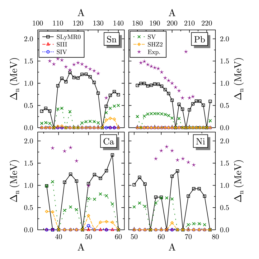
Figure 1: Neutron spectral gaps of singly magic even-even nuclei in the isotopic chains as indicated at the SR-EDF level.

In Fig. 1, pairing properties are examined via the spectral gap $E_{\text{pair},n}/\int\!d^{3}r\;\tilde{\rho}_{n}({\mathbf{r}})$ of neutrons as obtained from spherical HFB-type SR calculations of singly magic even-even nuclei. Empirical pairing gaps obtained from a three-point mass difference are shown for comparison. When solving HFB equations, pairing matrix elements have been multiplied with a smooth cutoff at $8.5$ MeV above and below the Fermi energy. SIII, SIV, SHZ2 and SV give null pairing or at least a weak pairing in some nuclei. Only SLyMR0, for which this property was enforced during the fit, provides pairing gaps of a realistic size.

Figure 2 exhibits mass residuals for isotopic and isotonic chains of singly magic nuclei as obtained from spherical HFB-type SR calculations. The particularly large drift of the curves obtained with SLyMR0 results mainly from its very low value for the asymmetry energy coefficient $a_{\text{sym}}$, which cannot be increased without jeopardising pairing or the time-odd terms in the EDF. We have checked that, in spite of its poor description of masses, SLyMR0 gives a reasonable description of the deformation of nuclei in the $sd$ and $pf$ shell regions, and of their rotational bands in cranked HFB calculations.

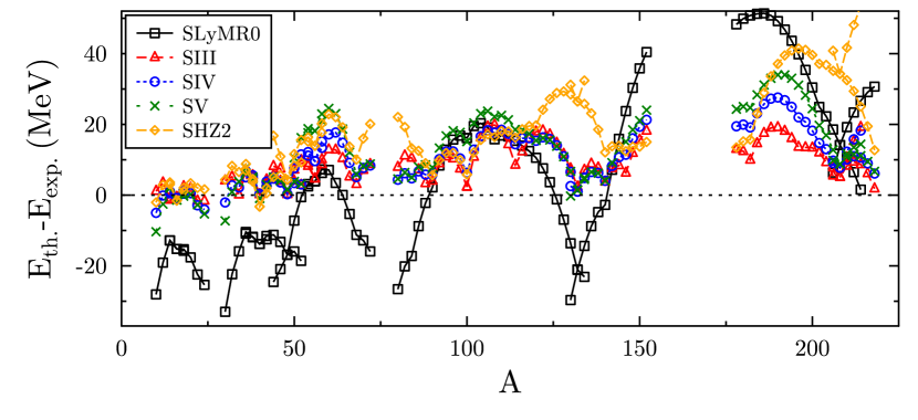
Figure 2: Binding energy residuals as a function of $A$ for singly magic nuclei for spherical SR-EDF calculations. Nuclei in isotonic and isotopic chains are connected by lines.

4 Conclusion

The simple pseudo-potential (2) allows for a description of basic nuclear properties that does not meet the standard of state-of-the-art SR-EDF calculations. However, it is sufficient for its main purpose of benchmarking multi-dimensional MR EDF calculations, which then will be free from the pathologies encountered with any modern standard parametrisation. In particular, we achieved a fair description of pair correlations while avoiding (finite-size) spin-instabilities. However, the simple form used here is clearly over-constrained and higher-order terms will be needed to replicate the performance of the best available general Skyrme EDFs at the SR level. Work in that direction is underway. As a first step, the most general central three-body contact operator up to second order in gradients has been worked out recently [25]. First fits that aim at the set-up of a suitable protocol are currently underway and show promising results.

Clarifying discussions with B. Avez, J. Meyer and A. Pastore are gratefully acknowledged. This work has been supported by the the Agence Nationale de la Recherche under Grant No. ANR 2010 BLANC 0407 ”NESQ”.

References

• [1] M. Bender, P.-H. Heenen and P.-G. Reinhard, Rev. Mod. Phys. 75 (2003) 121
• [2] P.-G. Reinhard and E. W. Otten, Nucl. Phys. A420 (1984) 173.
• [3] M. Bender, Eur. Phys. J ST 156 (2008) 217.
• [4] P. Ring and P. Schuck, The Nuclear Many-Body Problem, (Springer, New York, Heidelberg, Berlin, 1980)
• [5] J. Dobaczewski, M. V. Stoitsov, W. Nazarewicz, and P.-G. Reinhard, Phys. Rev. C 76 (2007) 054315.
• [6] D. Lacroix, T. Duguet, and M. Bender, Phys. Rev. C 79 (2009) 044318.
• [7] M. Anguiano, J. L. Egido, and L. M. Robledo, Nucl. Phys. A696 (2001) 467.
• [8] M. Bender, T. Duguet, and D. Lacroix, Phys. Rev. C 79 (2009) 044319.
• [9] T. Duguet, M. Bender, K. Bennaceur, D. Lacroix, and T. Lesinski, Phys. Rev. C 79 (2009) 044320.
• [10] T. Duguet, J. Sadoudi, J. Phys. G 37 (2010) 064009.
• [11] K. Washiyama, K. Bennaceur, B. Avez, M. Bender, P.-H. Heenen, and V. Hellemans, Phys. Rev. C 86 (2012) 054309.
• [12] T. H. R. Skyrme, Phil. Mag. 1 (1956) 1043.
• [13] S. O. Bäckman, A. D. Jackson, and J. Speth, Phys. Lett. B 56 (1975) 209.
• [14] E. Chabanat, J. Meyer, P. Bonche, R. Schaeffer, and P. Haensel, Nucl. Phys. A627 (1997) 710; ibid. A635 (1998) 231; ibid. A643 (1998) 441(E).
• [15] S. A. Fayans, S. V. Tolokonnikov, E. L. Trykov, and D. Zawischa, Nucl. Phys. A676 (2000) 49.
• [16] M. Baldo, P. Schuck and X. Viñas, Phys. Lett. B 663 (2008) 390.
• [17] J. P. Perdew and A. Zunger, Phys. Rev. B 23 (1981) 5048.
• [18] S. Stringari and D. M. Brink, Nucl. Phys. A304 (1978) 307.
• [19] E. Perlińska, S. G. Rohoziński, J. Dobaczewski, and W. Nazarewicz, Phys. Rev. C 69 (2004) 014316.
• [20] T. Lesinski, K. Bennaceur, T. Duguet and J. Meyer, Phys. Rev. C 74 (2006) 044315.
• [21] A. Pastore, D. Davesne, K. Bennaceur, J. Meyer, and V. Hellemans, contribution to this volume.
• [22] M. Beiner, H. Flocard, Nguyen Van Giai, and P. Quentin, Nucl. Phys. A238 (1975) 29.
• [23] W. Satuła, J. Dobaczewski, W. Nazarewicz, and M. Rafalski, Phys. Rev. C 81 (2010) 054310.
• [24] W. Satuła, J. Dobaczewski, W. Nazarewicz, and T. R. Werner, Phys. Rev. C 86 (2012) 054316.
• [25] J. Sadoudi, Thèse, Université Paris-Sud XI (2011).