Energy dependence of the entanglement entropy of composite boson (quasiboson) systems

Abstract

Bipartite composite boson (quasiboson) systems, which admit realization in terms of deformed oscillators, were considered in our previous paper from the viewpoint of entanglement characteristics. These characteristics, including entanglement entropy and purity, were expressed through the relevant deformation parameter for different quasibosonic states. On the other hand, it is of interest to present the entanglement entropy and likewise the purity as function of energy for those states. In this work, the corresponding dependencies are found for different states of composite bosons realized by deformed oscillators and, for comparison, also for the hydrogen atom viewed as composite boson. The obtained results are expressed graphically and their implications discussed.

I Introduction

Composite bosons or quasibosons or cobosons, as non-elementary systems or (quasi-)particles built from two or more constituent particles, are widely encountered Tichy et al. (2011); Avancini and Krein (1995); Hadjimichef et al. (1998); Perkins (2002); Keldysh and Kozlov (1968); Moskalenko and Snoke (2000); Bethe and Salpeter (1957) in diverse branches of modern theoretical (quantum) physics. Among quasibosons there are mesons, diquarks/tetraquarks, odd-odd or even-even nuclei, positronium, excitons, cooperons, atoms, etc. In the present work we focus on the case of bipartite (two-component) composite bosons. Their creation and annihilation operators can be given through the typical ansatz, $A^{{\dagger}}_{\alpha}=\sum_{\mu\nu}\Phi_{\alpha}^{\mu\nu}a^{{\dagger}}_{\mu}b^{{\dagger}}_{\nu},\ \ A_{\alpha}=\sum_{\mu\nu}\overline{\Phi_{\alpha}^{\mu\nu}}b_{\nu}a_{\mu}$, where $a^{{\dagger}}_{\mu}$ and $b^{{\dagger}}_{\nu}$ are the creation operators for the (distinguishable) constituents, which can be either both fermionic or both bosonic. In Gavrilik et al. (2011, 2011) it was shown that the composite bosons of particular form (i.e. those that involve appropriate matrices $\Phi_{\alpha}^{\mu\nu}$) can be realized, in algebraic sense, by suitable deformed bosons (deformed oscillators).

As known, among the measures characterizing degree of entanglement or correlation between the entangled constituents in a quasiboson there are Schmidt rank, Schmidt number, concurrence, purity, and the entanglement entropy. The latter two are especially important in the context of (theoretical and experimental) quantum information research, quantum communication and teleportation Horodecki et al. (2009); Tichy et al. (2011).

It is very important to know how the change of system’s energy influences the quantum correlation and/or quantum statistics properties of the system under study. As it is known, the characteristics of the entanglement between constituents of quasiboson, which measure bosonic quality of quasiboson Law (2005); Chudzicki et al. (2010); Ramanathan et al. (2011); Morimae (2010), and their energy dependence are of importance in quantum information research: the quantum communication, entanglement production Weder (2011), quantum dissociation processes Esquivel et al. (2011), particle addition or subtraction in general and in teleportation problem Kurzynski et al. (2012); Bartley et al. (2012), etc. The knowledge of the energy dependence of witnesses of quantum correlations e.g. entanglement entropy or purity allows one to relate these latter to the energy level of excitation that can be measured in the experiments, see e.g. Chang et al. (2012); Navarrete-Benlloch et al. (2012); Esquivel et al. (2011).

In other words, the energy of a quasiboson differs from the energy of the respective ideal boson by a term which depends on the quasiboson’s entanglement – the measure of deviation from bosonic behavior. All this motivates to study the energy dependence of the entanglement entropy and other witnesses of entanglement. In the present work we analyze interconnection between the energy of system (state) and such main two entanglement characteristics as entanglement entropy or purity. Note that the relationship between the entanglement and energy for composite bosons was discussed in Majtey et al. (2012); Bouvrie et al. (2011), for qubits in McHugh et al. (2006); Cavalcanti et al. (2006), and for spin systems in Wang et al. (2005).

For those composite bosons realizable by deformed oscillators it is possible, as shown in Gavrilik and Mishchenko (2012), to link directly the relevant parameter of deformation with the entanglement characteristics of the composite bosons. Namely, the characteristics (or measures) of bipartite entanglement with respect to $a$- and $b$-subsystems, see the above ansatz, were found explicitly Gavrilik and Mishchenko (2012) for single composite boson, for multi-quasiboson states, and for a coherent state, corresponding to the quasibosons system under study.

Among the above mentioned entanglement characteristics the entanglement entropy $S_{ent}$ certainly is of primary interest. Therefore in this work main attention is devoted to finding the explicit dependence of entanglement entropy $S_{ent}$ on the energy $E$ of the quasibosons system i.e. of the corresponding state. Present paper further develops the findings of Gavrilik and Mishchenko (2012): we take the composite bosons system as being realized in terms of independent-modes deformed oscillators with the quadratic structure function $\varphi(n)=\Bigl{(}1+\epsilon\frac{f}{2}\Bigr{)}n-\epsilon\frac{f}{2}n^{2}$, where $\epsilon=+1/-1$ for fermionic/bosonic constituents respectively. Our analysis here is performed for the states considered as the examples in Gavrilik and Mishchenko (2012), and also for the hydrogen atom as an independent example. The obtained dependences $S_{ent}(E)$ of the entanglement entropy on energy are shown graphically for a few values of the deformation parameter $f$; one of the cases is compared with the situation emerging for the hydrogen atom.

Analogous treatment, although in a shorter fashion is also performed for the purity-energy dependence. About the structure of the paper: in the next Sec. II we sketch some facts necessary for what follows; main results on the energy dependence of the entanglement entropy of (multi-)quasiboson states are presented in Sec. III and IV, whereas similar treatment for the purity witness of bipartite entanglement is given in Section V. The paper ends with discussion of the obtained results and of the most interesting from our viewpoint physical implications (sec. VI).

II Preliminaries

As already mentioned, we deal with composite bosons, which are realized by mode-independent system of deformed bosons (deformed oscillators) given for one mode by the structure function $\varphi(n)$. That means that algebraically the quasiboson operators $A_{\alpha}$, $A^{\dagger}_{\alpha}$ and the number operator $N_{\alpha}$ satisfy on the states the same relations as the corresponding deformed oscillator creation, annihilation and occupation number operators:

$$A^{\dagger}_{\alpha}A_{\alpha}=\varphi(N_{\alpha}),$$ (1)

$$[A_{\alpha},A^{\dagger}_{\beta}]=\delta_{\alpha\beta}\bigl{(}\varphi(N_{\alpha}+1)-\varphi(N_{\alpha})\bigr{)},$$ (2)

$$[N_{\alpha},A^{\dagger}_{\beta}]=\delta_{\alpha\beta}A^{\dagger}_{\beta},\quad[N_{\alpha},A_{\beta}]=-\delta_{\alpha\beta}A_{\beta},$$ (3)

where the Kronecker deltas reflect mode-independence. Such a realization is possible, see Gavrilik et al. (2011, 2011), only when the structure function $\varphi(n)$ involving discrete deformation parameter $f$ is quadratic in $n$, namely (recall that $\epsilon=\pm 1$)

$$\varphi(n)=\Bigl{(}1+\epsilon\frac{f}{2}\Bigr{)}n-\epsilon\frac{f}{2}n^{2},\quad f=\frac{2}{m},\ \ m\in\mathds{N},$$ (4)

whereas the matrices $\Phi_{\alpha}$, are of the form:

$$\Phi_{\alpha}=U_{1}(d_{a})\mathop{\mathrm{diag}}\nolimits\Bigl{\{}0..0,\sqrt{f/2}\,U_{\alpha}(m),0..0\Bigr{\}}U^{{\dagger}}_{2}(d_{b}).$$ (5)

Note that the state of one composite boson

$$|\Psi_{\alpha}\rangle\!=\!\sum_{\mu\nu}\Phi_{\alpha}^{\mu\nu}|a_{\mu}\rangle\!\otimes\!|b_{\nu}\rangle,\ \ |a_{\mu}\rangle\equiv a^{{\dagger}}_{\mu}|0\rangle,\ |b_{\nu}\rangle\equiv b^{{\dagger}}_{\nu}|0\rangle,$$ (6)

see ansatz, is in general bipartite entangled with respect to the states of two constituent fermions (or two bosons); likewise, the state describing many composite bosons,

$$|\Psi\rangle=\sum\limits_{\{n_{\gamma}\}}\Psi\bigl{(}\{n_{\gamma}\}\bigr{)}(A^{{\dagger}}_{\gamma_{1}})^{n_{\gamma_{1}}}\cdot...\cdot(A^{{\dagger}}_{\gamma_{D}})^{n_{\gamma_{D}}}|0\rangle$$ (7)

is viewed as bipartite entangled with respect to $a$- and $b$-subsystems. The degree of entanglement can be measured by such well-known characteristics as Schmidt rank, Schmidt number, purity, entanglement entropy and concurrence, see e.g. Tichy et al. (2011); Horodecki et al. (2009) for their definition.

For the entanglement entropy in the case of one composite boson we obtain Gavrilik and Mishchenko (2012),

$$S_{\rm ent}=\ln(m)=\ln\frac{2}{f},$$ (8)

whereas for the multi-quasibosonic states (7), see Gavrilik and Mishchenko (2012),

$$S_{\rm ent}=-\sum\limits_{\{n_{\gamma}\}}|\Psi\bigl{(}\{n_{\gamma}\}\bigr{)}|^{2}\Bigl{(}\frac{1}{m}\Bigr{)}^{\sum\limits_{j=1}^{D}n_{\gamma_{j}}}\prod\limits_{j=1}^{D}(n_{\gamma_{j}}!)^{2}N_{m}^{n_{\gamma_{j}}}\cdot$$

$$\cdot\ln\biggl{[}|\Psi\bigl{(}\{n_{\gamma}\}\bigr{)}|^{2}\Bigl{(}\frac{1}{m}\Bigr{)}^{\sum\limits_{j=1}^{D}n_{\gamma_{j}}}\prod\limits_{j=1}^{D}(n_{\gamma_{j}}!)^{2}\biggr{]}.$$ (9)

III Energy dependence of the entanglement entropy

In order to find the energy dependence of the entanglement entropy we need the expression for the Hamiltonian of the composite boson system. Different choices are possible here, but, since quasibosons in our approach are realized by means of deformed oscillators, we adopt the corresponding Hamiltonian of the same form as e.g. in Gavrilik and Rebesh (2008, 2008). That is, we take the following Hamiltonian of deformed oscillators (deformed bosons) which provide realization of the composite bosons:

$$H=\sum_{\alpha}\frac{1}{2}\hbar\omega_{\alpha}\bigl{(}\varphi(N_{\alpha})+\varphi(N_{\alpha}+1)\bigr{)}.$$ (10)

Single composite boson (quasiboson) case.

As our first example, consider the system which consists of single composite boson. For the entanglement entropy in this case we have Gavrilik and Mishchenko (2012)

$$S_{\rm ent}=\ln\frac{2}{f}.$$ (11)

The expression for the energy of one composite boson as follows from (10) along with (4), is

$$E=\frac{\hbar\omega}{2}\bigl{(}\varphi(1)+\varphi(2)\bigr{)}=\hbar\omega\Bigl{(}\frac{3}{2}-\epsilon\frac{f}{2}\Bigr{)}=\hbar\omega\bigl{(}\frac{3}{2}-\frac{\varepsilon}{m}\bigr{)}.$$ (12)

Then for the entanglement entropy characterizing single composite boson we find

$$S_{\rm ent}=\ln\frac{\epsilon}{\frac{3}{2}-\frac{E}{\hbar\omega}}=$$

$$=\left\{\begin{aligned} &-\ln\Bigl{(}\frac{3}{2}-\frac{E}{\hbar\omega}\Bigr{)},\ \epsilon=1,\ \ \frac{1}{2}\leq\frac{E}{\hbar\omega}\leq\frac{3}{2},\\ &-\ln\Bigl{(}\frac{E}{\hbar\omega}-\frac{3}{2}\Bigr{)},\ \epsilon=-1,\ \ \frac{3}{2}\leq\frac{E}{\hbar\omega}\leq\frac{5}{2}.\end{aligned}\right.$$ (13)

The plots corresponding to eq. (III) are presented on Fig.1, Fig.2. Note the important feature of the opposite behavior (increasing vs decreasing) of the energy dependence in the case of fermionic constituents with respect to the case of bosonic constituents. In the both $\varepsilon=\pm 1$ cases the entropy $S_{\rm ent}$ goes to infinity for the energy $E=\frac{3}{2}\hbar\omega$, which implies maximal entanglement between constituents. In this case the constituents (fermionic or bosonic) become most tightly bound within a quasiboson, and the quasiboson is most close to pure boson. On the contrary for $E=\frac{1}{2}\hbar\omega$, $\varepsilon=+1$, and $E=\frac{5}{2}\hbar\omega$, $\varepsilon=-1$, the entanglement entropy $S_{\rm ent}=0$ i.e. the constituents are unentangled. From physical viewpoint, in this case the constituents are in fact unbound.

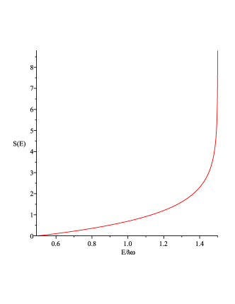
Figure 1: Dependence of the entanglement entropy $S_{\rm ent}$ on the energy $E_{\alpha}$ for a single composite boson in the case of fermionic components i.e. at $\epsilon=+1$.

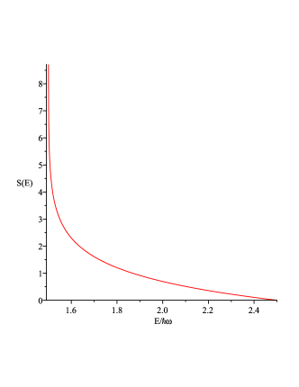
Figure 2: Dependence of the entanglement entropy $S_{\rm ent}$ on the energy $E_{\alpha}$ for a single composite boson in the case of bosonic components i.e. at $\epsilon=-1$.

Hydrogen atom as quasiboson.

It is of interest to consider the hydrogen atom which constitutes a composite boson (entangled with respect to proton and electron). In this case, however, the relevant matrices $\Phi_{\alpha}^{\mu\nu}$ are not of the form (5), therefore if it (H-atom) was realized by a deformed boson (this is an open problem), the latter should be different from the type mentioned above. So, the creation operator for the hydrogen atom with zero total momentum and quantum number $n$ can be written in second quantization formalism (with discrete momenta) as

$$A^{\dagger}_{{\bf 0}n}=\frac{(2\pi\hbar)^{3/2}}{\sqrt{V}}\sum_{\bf p}\phi_{{\bf p}n}a^{\dagger}_{\bf p}b^{\dagger}_{-\bf p},$$ (14)

where $a^{\dagger}_{\bf p}$ and $b^{\dagger}_{-\bf p}$ are the creation operators for electron and proton respectively taken with opposite momenta; $V$ is large enough confining volume for the hydrogen atom. The momentum-space wavefunction $\phi_{{\bf p}n}$ is determined by the Schrodinger equation:

$$\phi_{{\bf p}n}=\int\frac{1}{(2\pi\hbar)^{3/2}}e^{\frac{i}{\hbar}{\bf pr}}\phi_{n}({\bf r})d^{3}{\bf r};$$

$$-\frac{\hbar^{2}\nabla^{2}}{2m}\phi_{n}({\bf r})+U({\bf r})\phi_{n}({\bf r})=E_{n}\phi_{n}({\bf r}).$$

The expression for the Hydrogen wavefunction in the momentum representation is given as Bethe and Salpeter (1957)

$$\phi_{{\bf p}nlm}\!=\!\frac{e^{\pm im\phi_{p}}}{(2\pi)^{1/2}}\Bigl{(}\frac{(2l\!+\!1)(l\!-\!m)!}{2(l\!+\!m)!}\Bigr{)}^{1/2}P^{m}_{l}(\cos\theta_{p})\frac{\pi 2^{2l+4}l!}{(\gamma h)^{3/2}}\cdot$$

$$\cdot\Bigl{(}\frac{n(n\!-\!l\!-\!1)!}{(n\!+\!l)!}\Bigr{)}^{1/2}\frac{\xi^{l}}{(\xi^{2}\!+\!1)^{l+2}}C^{l+1}_{n-l-1}\Bigl{(}\frac{\xi^{2}\!-\!1}{\xi^{2}\!+\!1}\Bigr{)},$$ (15)

where $P^{m}_{l}$ is the associated Legendre polynomial, $C^{l+1}_{n-l-1}(...)$ is Gegenbauer polynomial, $\xi=(2\pi/\gamma h)p$, $\gamma=Z/na_{0}$.

The expansion (14) can be viewed directly as the Schmidt decomposition for the state $A^{\dagger}_{{\bf 0}n}|0\rangle$ with Schmidt coefficients $\lambda_{\bf p}=\frac{(2\pi\hbar)^{3/2}}{\sqrt{V}}\phi_{{\bf p}n}$. Then the entanglement entropy for the hydrogen atom is given by the relation

$$S_{\rm ent}=-\sum_{\bf p}|\lambda_{\bf p}|^{2}\ln|\lambda_{\bf p}|^{2}=$$

$$=-\sum_{\bf p}\frac{(2\pi\hbar)^{3}}{V}|\phi_{{\bf p}n}|^{2}\ln\Bigl{(}\frac{(2\pi\hbar)^{3}}{V}|\phi_{{\bf p}n}|^{2}\Bigr{)},$$ (16)

where the first equality is nothing but the definition of the entanglement entropy Tichy et al. (2011).

Calculation of the expression (16) is moved to appendix. Performing derivation we obtain the following result

$$S_{\rm ent}=-\ln\Bigl{[}\frac{(2l+1)(l-m)!}{(l+m)!}\frac{4\pi 2^{2l}(l!)^{2}}{V(na_{0})^{-3}}\frac{n(n-l-1)!}{(n+l)!}\Bigr{]}-\\ -\frac{(2l+1)(l-m)!}{2(l+m)!}\,\int\limits_{-1}^{1}dt|P^{m}_{l}(t)|^{2}\ln|P^{m}_{l}(t)|^{2}-\\ \!-\!\frac{4^{l}(l!)^{2}}{\pi/2}\frac{n(n\!-\!l\!-\!1)!}{(n+l)!}\!\int\limits_{-1}^{1}\!dx\frac{\sqrt{1\!-\!x^{2}}\!}{(1\!-\!x)^{3}}G_{nl}\!(x)\ln G_{nl}\!(x),$$ (17)

where $G_{nl}(x)=(1-x^{2})^{l}(1-x)^{4}\bigl{(}C^{l+1}_{n-l-1}(x)\bigr{)}^{2}$. Let us consider the simplest case when the quantum numbers $l=0$ and $m=0$. For these values,

$$S_{\rm ent}=\ln\Bigl{[}\frac{V}{4\pi n^{3}a_{0}^{3}}\Bigr{]}-\frac{2}{\pi}\int\limits_{-1}^{1}dx(1-x^{2})^{1/2}(1-x)\bigl{(}C^{1}_{n-1}(x)\bigr{)}^{2}\cdot\\ \cdot\ln\Bigl{[}(1-x)^{4}\bigl{(}C^{1}_{n-1}(x)\bigr{)}^{2}\Bigr{]}=S_{\rm ent}^{(0)}-\ln[4\pi n^{3}]-\\ -\frac{2}{\pi}\!\int\limits_{-1}^{1}\!dx(1-x^{2})^{1/2}(1-x)\bigl{(}C^{1}_{n\!-\!1}(x)\bigr{)}^{2}\cdot\\ \cdot\ln\Bigl{[}(1-x)^{4}\bigl{(}C^{1}_{n\!-\!1}(x)\bigr{)}^{2}\Bigr{]},\qquad S_{\rm ent}^{(0)}=\ln\frac{V}{a_{0}^{3}}.$$ (18)

Making replacement $x=\cos\alpha$ in the integral in (18), and using the formula $C_{n-1}^{1}(\cos\alpha)=\frac{\sin(n\alpha)}{\sin\alpha}$, we infer:

$$S_{\rm ent}=S_{\rm ent}^{(0)}-\ln[4\pi n^{3}]-\frac{2}{\pi}\int\limits_{0}^{\pi}d\alpha(1-\cos\alpha)\sin^{2}(n\alpha)\cdot\\ \cdot\ln\Bigl{[}(1-\cos\alpha)^{4}\frac{\sin^{2}(n\alpha)}{\sin^{2}\alpha}\Bigr{]}$$ (19)

From the well-known expression for the energy of H-atom, $E=-{\rm Ry}/n^{2}$, we have $n=\sqrt{-{\rm Ry}/E}$. Substituting this in (19) we finally obtain

$$\Delta S(E)=S_{\rm ent}(E)-S_{\rm ent}^{(0)}=-\ln\Bigl{[}4\pi\Bigl{(}-\frac{\rm Ry}{E}\Bigr{)}^{3/2}\Bigr{]}-\\ -\frac{2}{\pi}\int\limits_{0}^{\pi}d\alpha(1-\cos\alpha)\sin^{2}\Bigl{(}\sqrt{-\frac{\rm Ry}{E}}\alpha\Bigr{)}\cdot\\ \cdot\ln\Bigl{[}(1-\cos\alpha)^{4}\frac{\sin^{2}\bigl{(}\sqrt{-\frac{\rm Ry}{E}}\alpha\bigr{)}}{\sin^{2}\alpha}\Bigr{]}$$ (20)

The derived energy dependence is shown graphically on Fig. 3. As seen, the character of the energy dependence here essentially differs from that of the single quasiboson (two-fermion composite) case above, see Fig.1. Main reason for distinction lies in that the matrices $\Phi_{\alpha}^{\mu\nu}$ of composite bosons realized by deformed oscillators are different from the corresponding matrices of hydrogen atom given by its wavefunction $\phi_{{\bf p}n}$. From the physics viewpoint this implies that the effective interaction between the constituents in the above quasiboson is different from the Coulomb interaction within hydrogen atom.

Of course, it would be useful to perform the analysis of H-atom system by taking into account the fact that the proton, in its turn, also has composite structure (three-quark system), thus differing from fundamental (elementary) fermionic entity.

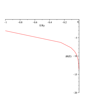
Figure 3: Dependence of the entanglement entropy $\Delta S=S_{\rm ent}-S_{\rm ent}^{(0)}$ from  (20) on the energy $E$ for Hydrogen atom.

Let us recall once more that the example of H-atom, treated as quasiboson, is included here for comparative purpose only. We suppose however that some realization (by deformed oscillators) for hydrogen atom as composite quasiboson does also exist, though it may be rather complicated and non-algebraic. In fact, this task is to be solved in two stages: first we have to construct a realization of 3-fermion (3-quark) state for the proton subsystem by some deformed fermionic oscillator, and, second, of a quasi-boson formed from the (protonic) quasifermion and one more fermion, i.e. electron. We hope to solve this very involved problem in near future.

IV Entanglement entropy vs energy for multi-quasiboson system

Now examine the case of multi-quasiboson states. Taking into account the Hamiltonian (10), the total energy of the system (at mode-independence) is expressed as

$$E=\sum_{\alpha}\hbar\omega_{\alpha}\Bigl{[}n_{\alpha}+\frac{1}{2}-\epsilon\frac{f}{2}n_{\alpha}^{2}\Bigr{]}.$$ (21)

Qusiboson Fock state.

Let us find the entanglement entropy as function of energy for the normalized Fock state of $n_{\alpha}$ quasibosons, $[\phi(n_{\alpha})!]^{-1/2}(A^{{\dagger}}_{\alpha})^{n_{\alpha}}|0\rangle$, in a fixed mode $\alpha$. The entropy of entanglement between $a$- and $b$-subsystems for the two values of $\epsilon$ equals respectively, see Gavrilik and Mishchenko (2012), to

$$S_{\rm ent}|_{\epsilon=+1}=\ln C_{2/f}^{n_{\alpha}},\quad S_{\rm ent}|_{\epsilon=-1}=\ln C_{2/f+n_{\alpha}-1}^{n_{\alpha}}.$$ (22)

The latter dependencies $S_{\rm ent}=S_{\rm ent}(n_{\alpha})$ are shown in Fig. 4 and Fig 5.

By inverting eq. (21) we have the dependence of the occupation number $n_{\alpha}$ of quasibosons in $\alpha$th mode on the corresponding energy $E_{\alpha}$ of quasibosons:

$$n^{\pm}_{\alpha}(E_{\alpha})=\frac{1\pm\sqrt{1-2\epsilon f\bigl{(}\frac{E_{\alpha}}{\hbar\omega_{\alpha}}-\frac{1}{2}\bigr{)}}}{2\epsilon f}.$$

Substitution of this expression in (22) leads us to the two-branch form of the concerned dependence $S^{\pm}_{\rm ent}(E_{\alpha})$ for the case $\epsilon=+1$:

$$S^{\pm}_{\rm ent}(E_{\alpha})|_{\epsilon=+1}=\ln\Bigl{(}C_{2/f}^{[1\pm\sqrt{1\!+\!f\!-\!2fE_{\alpha}/\hbar\omega_{\alpha}}\,]/(2f)}\Bigr{)},$$ (23)

where $\frac{E}{\hbar\omega}\leq\frac{1\!+\!f}{2f}$ for both $S^{+}_{\rm ent}$ and $S^{-}_{\rm ent}$ branches, and $\frac{E}{\hbar\omega}\geq\frac{1}{2}$ for the $S^{-}_{\rm ent}$-branch. For $\epsilon=-1$ we have single monotonous branch:

$$S_{\rm ent}(E_{\alpha})|_{\epsilon=-1}\!=\!\ln\Bigl{(}\!C_{2/f\!-\!1+[\sqrt{1\!-\!f\!+\!2fE_{\alpha}/\hbar\omega_{\alpha}}\!-\!1]/(2f)}^{[\sqrt{1\!-\!f\!+\!2fE_{\alpha}/\hbar\omega_{\alpha}}-1]/(2f)}\!\Bigr{)},$$ (24)

where $\frac{E}{\hbar\omega}\!\geq\!\frac{1}{2}$. The corresponding functions are presented graphically in Fig. 6 and Fig. 7.

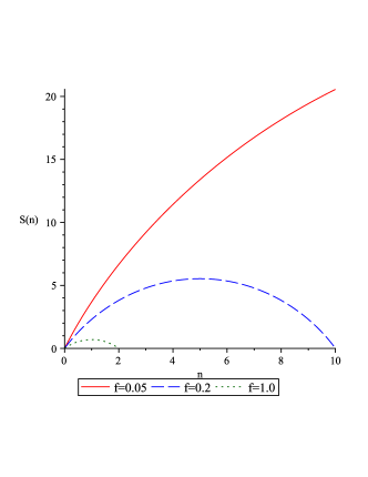
Figure 4: Dependence of the entanglement entropy $S_{\rm ent}$, see (22), on the number of quasibosons $n_{\alpha}$ for one-mode multi-quasibosonic system: the case $\epsilon=+1$ of fermionic components.

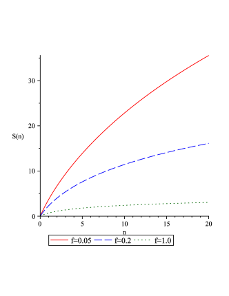
Figure 5: Dependence of the entanglement entropy $S_{\rm ent}$, see (22), on the number of quasibosons $n_{\alpha}$ for one-mode multi-quasibosonic system: the case $\epsilon=-1$ of bosonic components.

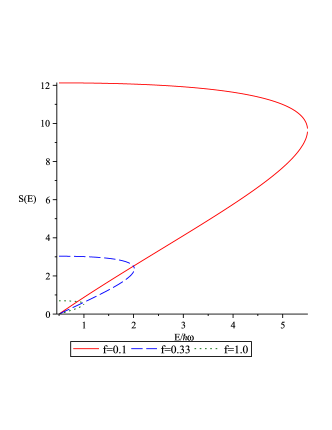
Figure 6: Dependence of the entanglement entropy $S_{\rm ent}$, see (23), on the energy $E_{\alpha}$ for one-mode multi-quasibosonic system: the case $\epsilon=+1$ of fermionic components.

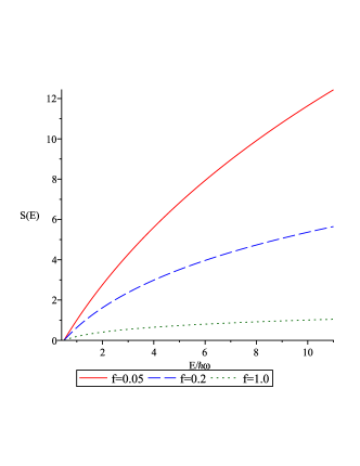
Figure 7: Dependence of the entanglement entropy $S_{\rm ent}$, see (24), on the energy $E_{\alpha}$ for one-mode multi-quasibosonic system: the case $\epsilon=-1$ of bosonic components.

The state with one quasiboson per mode.

Now let us turn to the Example 2 from Gavrilik and Mishchenko (2012). In this case the quasibosons are all in different modes, i.e. the quasibosonic system is in the state

$$|\Psi\rangle=A^{{\dagger}}_{\gamma_{1}}\cdot...\cdot A^{{\dagger}}_{\gamma_{n}}|0\rangle,\quad\gamma_{i}\neq\gamma_{j},\ i\neq j,\ i,j=1,...,n.$$

For the entanglement entropy, for $\epsilon=\pm 1$, we have

$$S_{\rm ent}=n\ln(m)=n\ln\frac{2}{f}.$$ (25)

The energy of the system depends on the dispersion relation of $\omega_{\gamma_{j}}$ as function of $\gamma_{j}$. Taking it in linear (in $\gamma_{j}$) form, namely $\omega_{\gamma_{j}}=\omega_{0}+(\gamma_{j}-\gamma_{1})\frac{\partial{\omega}}{\partial{\gamma}}$, and also using (21) and $n_{\gamma_{j}}=1$, we arrive at the following expression for the energy:

$$E=\frac{3-\epsilon f}{2}\bigl{(}\hbar\omega_{0}n+\frac{1}{2}\hbar\omega n(n-1)\bigr{)},$$ (26)

where $\delta\omega=\frac{\partial{\omega}}{\partial{\gamma}}\delta\gamma$. Solving the latter yields $n$ as function of energy, namely

$$n(E)=\frac{-1+\frac{1}{2}\frac{\delta\omega}{\omega_{0}}+\sqrt{\bigl{(}1-\frac{1}{2}\frac{\delta\omega}{\omega_{0}}\bigr{)}^{2}+4\frac{\delta\omega}{\omega_{0}}\frac{1}{3-\epsilon\!f}\frac{E}{\hbar\omega_{0}}}}{\delta\omega/\omega_{0}}.$$ (27)

Then (25) yields

$$S_{\rm ent}(E)\!=\!\frac{-1\!+\!\frac{1}{2}\frac{\delta\omega}{\omega_{0}}\!+\!\sqrt{\bigl{(}1\!-\!\frac{1}{2}\frac{\delta\omega}{\omega_{0}}\bigr{)}^{2}\!+\!4\frac{\delta\omega}{\omega_{0}}\frac{1}{3-\epsilon\!f}\frac{E}{\hbar\omega_{0}}}}{\delta\omega/\omega_{0}}\,\ln\frac{2}{f}.$$ (28)

Like in the previous case we obtain the corresponding plots which are now placed in Fig. 8 and Fig. 9 ($S$ is given in units of $\omega/\delta\omega$ and $E$ in units of $\hbar\omega^{2}/\delta\omega$; besides, $\omega=|\omega_{0}-\frac{1}{2}\delta\omega|$ is put).

).

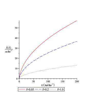
Figure 8: Dependence of the entanglement entropy $S_{\rm ent}$ on energy $E$ for multi-quasibosonic system with one quasiboson per mode: the case $\epsilon=+1$ of fermionic constituents.

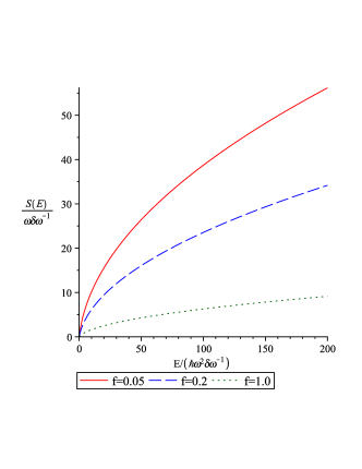
Figure 9: Dependence of the entanglement entropy $S_{\rm ent}$ on energy $E_{\alpha}$ for multi-quasibosonic system with one quasiboson per mode: the case $\epsilon=-1$ of bosonic constituents.

Coherent state of quasibosons.

As our last example consider the coherent state of composite bosons system in $\alpha$th mode, see Example 3 in Gavrilik and Mishchenko (2012):

$$|\Psi_{\alpha}\rangle\!=\!\tilde{C}(\mathcal{A};m)\sum\limits_{n=0}^{\infty}\frac{\mathcal{A}^{n}}{\phi(n)!}(A^{{\dagger}}_{\alpha})^{n}|0\rangle,$$ (29)

$$\tilde{C}(\mathcal{A};m)\!=\!\biggl{(}\sum\limits_{n=0}^{\infty}\frac{|\mathcal{A}|^{2n}}{\phi(n)!}\biggr{)}^{-1/2}\!\!=\!\biggl{[}\frac{(m\!-\!1)!I_{m-1}(z)}{(z/2)^{m-1}}\biggr{]}^{-\frac{1}{2}}=$$

$$=\mathrm{e}^{-|\mathcal{A}|^{2}/2}\Bigl{[}1+\frac{1}{4}\frac{|\mathcal{A}|^{4}}{m}+...\Bigr{]},\ \ \ z=2\sqrt{m}|\mathcal{A}|,$$

where $I_{m-1}(z)$ is the modified Bessel function of order $m\!-\!1$. For mean energy of the system in this state we have

$$E_{\alpha}=\langle\Psi_{\alpha}|\frac{1}{2}\hbar\omega_{\alpha}[\varphi(N_{\alpha})+\varphi(N_{\alpha}+1)]|\Psi_{\alpha}\rangle=\frac{1}{2}\hbar\omega_{\alpha}|\tilde{C}|^{2}\cdot\\ \cdot\sum_{n=0}^{\infty}\frac{|\mathcal{A}|^{2n}}{\varphi(n)!}\varphi(n)+\frac{1}{2}\hbar\omega_{\alpha}|\tilde{C}|^{2}\sum_{n=0}^{\infty}\frac{|\mathcal{A}|^{2n}}{\varphi(n)!}\varphi(n+1)=\\ =\hbar\omega_{\alpha}|\tilde{C}|^{2}|\mathcal{A}|^{2}\sum_{n=0}^{\infty}\frac{|\mathcal{A}|^{2n}}{\varphi(n)!}+\frac{1}{2}\hbar\omega_{\alpha}|\tilde{C}|^{2}\sum_{n=0}^{\infty}\frac{|\mathcal{A}|^{2n}}{\varphi(n)!}\cdot\\ \cdot[\varphi(n+1)-\varphi(n)]=\hbar\omega_{\alpha}|\mathcal{A}|^{2}+\frac{1}{2}\hbar\omega_{\alpha}|\tilde{C}|^{2}\sum_{n=0}^{\infty}\frac{|\mathcal{A}|^{2n}}{\varphi(n)!}\Bigl{[}1+\frac{2n}{m}\Bigr{]}\\ =\hbar\omega_{\alpha}|\mathcal{A}|^{2}+\frac{1}{2}\hbar\omega_{\alpha}+\frac{1}{2}\hbar\omega_{\alpha}\frac{1}{m}|\tilde{C}|^{2}|\mathcal{A}|\frac{\partial{}}{\partial{|\mathcal{A}|}}\sum_{n=0}^{\infty}\frac{|\mathcal{A}|^{2n}}{\varphi(n)!}=\\ =\hbar\omega_{\alpha}\bigl{(}|\mathcal{A}|^{2}+1/2\bigr{)}+\frac{1}{2}\hbar\omega_{\alpha}\frac{1}{m}|\mathcal{A}|\frac{\partial{}}{\partial{|\mathcal{A}|}}\ln\frac{I_{m-1}(z)}{|\mathcal{A}|^{m-1}}=\\ =\hbar\omega_{\alpha}\bigl{(}|\mathcal{A}|^{2}+\frac{1}{2}\bigr{)}+\hbar\omega_{\alpha}\frac{1}{\sqrt{m}}|\mathcal{A}|\frac{I^{\prime}_{m-1}(z)}{I_{m-1}(z)}-\frac{1}{2}\hbar\omega_{\alpha}\frac{1}{m}(m-1)=\\ =\hbar\omega_{\alpha}\Bigl{(}|\mathcal{A}|^{2}\!+\!\frac{1}{2m}\Bigr{)}+\frac{\hbar\omega_{\alpha}|\mathcal{A}|}{\sqrt{m}}\frac{I_{m}(2\sqrt{m}|\mathcal{A}|)\!+\!I_{m-2}(2\sqrt{m}|\mathcal{A}|)}{2I_{m-1}(2\sqrt{m}|\mathcal{A}|)}$$ (30)

The entanglement entropy for the coherent state (29) is given, see Gavrilik and Mishchenko (2012), by the formula (recall that $m=\frac{2}{f}$):

$$S_{\rm ent}=\tilde{C}^{2}\sum\limits_{n=0}^{\infty}\frac{(|\mathcal{A}|^{2}m)^{n}}{(n!)^{2}C^{n}_{n+m-1}}\ln\biggl{[}\frac{(n!)^{2}(C_{n+m-1}^{n})^{2}}{\tilde{C}^{2}(|\mathcal{A}|^{2}m)^{n}}\biggr{]}.$$ (31)

Hence we have nothing but the dependence of $S_{\rm ent}$ on $E_{\alpha}$ in parametric form (unfortunately, we cannot solve (30) for $|\mathcal{A}|$, here $|\mathcal{A}|$ being the parameter, in order to insert the solution into (31); that is why we merely use parametric presentation of the $S_{\rm ent}=S_{\rm ent}(E)$ dependence). The plot of this dependence is given in Fig. 10.

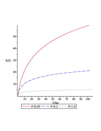
Figure 10: Dependence of the entanglement entropy $S_{\rm ent}$ in (31) on the mean energy $E_{\alpha}$, see (30), for quasibosonic coherent state.

V Energy dependence of other measures (witnesses) of entanglement

There exist some other widely used witnesses of entanglement: Schmidt rank, concurrence, Schmidt number $K$ or its inverse $P=1/K$ termed purity Tichy et al. (2011); Horodecki et al. (2009). Energy dependence of these entanglement witnesses, Schmidt rank, concurrence and purity have somewhat simpler form and can be calculated in a similar way using explicit formulas from Gavrilik and Mishchenko (2012).

Since such entanglement characteristics as purity is exploited in connection with the issue of entanglement creation in scattering processes Weder (2011) and others Kurzynski et al. (2012); McHugh et al. (2006), let us pay some attention to $P$.

For the entangled system consisting of one quasiboson the purity in Gavrilik and Mishchenko (2012) was found to be connected with the deformation parameter $m=\frac{2}{f}$ in a simple way:

$$P\!=\!\sum_{k}\lambda_{k}^{4}\!=\!\frac{1}{m},\ \text{or}\ P\!=\!\mathop{\mathrm{Tr}}\nolimits(\rho_{\alpha}^{(a)})^{2}\!=\!\mathop{\mathrm{Tr}}\nolimits(\rho_{\alpha}^{(b)})^{2}\!=\!\frac{1}{m}.$$ (32)

Then, the energy dependence for purity in case of a single composite boson readily follows by combining (32) with (12) that gives:

$$P=\frac{f}{2}=\frac{1}{\epsilon}\Bigl{(}\frac{3}{2}-\frac{E}{\hbar\omega}\Bigr{)}=$$

$$=\left\{\begin{aligned} &\Bigl{(}\frac{3}{2}-\frac{E}{\hbar\omega}\Bigr{)},\ \epsilon=1,\ \ \frac{1}{2}\leq\frac{E}{\hbar\omega}\leq\frac{3}{2},\\ &\Bigl{(}\frac{E}{\hbar\omega}-\frac{3}{2}\Bigr{)},\ \epsilon=-1,\ \ \frac{3}{2}\leq\frac{E}{\hbar\omega}\leq\frac{5}{2}.\end{aligned}\right.$$ (33)

Thus, the dependence of purity on energy is linear for both $\varepsilon=+1$ and $\varepsilon=-1$. Observe however the two mutually opposite (i.e. falling versus raising) types of behavior of purity with increasing energy in the cases of fermionic versus bosonic constituents.

In a similar way, for purity in the case of single-mode multi-quasibosonic Fock states on the base of Gavrilik and Mishchenko (2012) we obtain

$$P^{\pm}_{\rm ent}(E_{\alpha})|_{\epsilon=+1}=\Bigl{(}C_{2/f}^{[1\pm\sqrt{1\!+\!f\!-\!2fE_{\alpha}/\hbar\omega_{\alpha}}\,]/(2f)}\Bigr{)}^{-1},$$ (34)

$$P_{\rm ent}(E_{\alpha})|_{\epsilon=-1}\!=\!\Bigl{(}\!C_{2/f\!-\!1+[\sqrt{1\!-\!f\!+\!2fE_{\alpha}/\hbar\omega_{\alpha}}\!-\!1]/(2f)}^{[\sqrt{1\!-\!f\!+\!2fE_{\alpha}/\hbar\omega_{\alpha}}-1]/(2f)}\!\Bigr{)}^{-1},$$ (35)

the definition intervals being the same as for the entanglement entropy, see (23) and (24). The functions (34) and (35) of energy are presented graphically in Fig. 11 and Fig. 12 correspondingly. Notice the peculiar shape of curves in Fig. 11 (non-monotonic behavior, with two pieces of monotonicity for each curve).

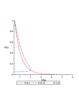
Figure 11: Dependence of the purity $P$, see (34), on the energy $E_{\alpha}$ for one-mode multi-quasibosonic system: the case $\epsilon=+1$ of fermionic components.

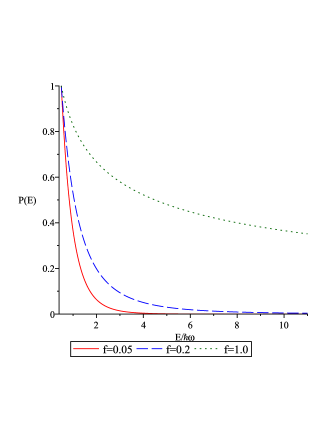
Figure 12: Dependence of the Purity $P$, see (35), on the energy $E_{\alpha}$ for one-mode multi-quasibosonic system: the case $\epsilon=-1$ of bosonic components.

Likewise, for multi-quasibosonic states with one quasiboson per mode, using the expression for purity calculated in Gavrilik and Mishchenko (2012) we easily find

$$P(E)=\exp(-S_{\rm ent}(E)).$$ (36)

The corresponding plots are now placed in Figs.13, 14.

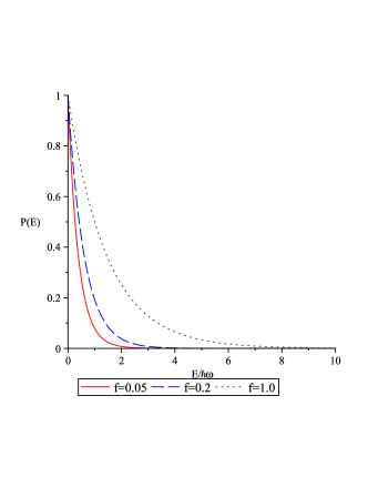
Figure 13: Dependence of the purity $P$ on energy $E$ for multi-quasibosonic system with one quasiboson per mode: the case $\epsilon=\!+\!1$ of fermionic constituents.

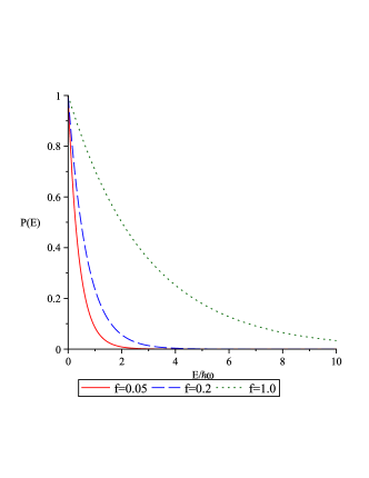
Figure 14: Dependence of the purity $P$ on energy $E_{\alpha}$ for multi-quasibosonic system with one quasiboson per mode: the case $\epsilon=\!-\!1$ of bosonic constituents.

As Figs. 12-14 demonstrate, purity is falling from its maximal possible value $P=1$ (zero entanglement) attained at $E=\frac{\hbar\omega}{2}$ implying absence of quanta, to $P=0$ at very large energies of many-particle states. A peculiar behavior of purity as function of energy is seen in Fig. 11: purity drops from $P=1$ with energy growing to some maximum $E_{\rm max}(f)$ (the latter is determined by the parameter $f$), then further decreases from $P_{f}\equiv P(E_{\rm max}(f))$ with the energy lowering from $E_{\rm max}(f)$ to smallest values. It is tempting to interpret such existence of two regimes as follows: both addition and subtraction Kurzynski et al. (2012),Bartley et al. (2012) of quanta (of quasiboson) can result in lowering purity. The two regimes, linked with existence of two branches, differ in the starting value of purity $P$ (whether it is zero or $P(E_{\rm max})$).

VI Discussion

In conclusion, let us make some comments on the obtained dependencies of entanglement entropy on energy, and their visualization with the corresponding plots. For the state of one composite boson realized by deformed oscillator, using the Hamiltonian (10) we find that the entanglement entropy monotonically grows with energy if the components are fermions, and decreases if the components are bosons (Figures 1 and 2).

We infer that for larger energies two-fermion quasiboson becomes more tightly bound whereas two-boson quasiboson becomes less bound. In the both cases the energy $E=\frac{3}{2}\hbar\omega$ corresponds to the most entangled quasiboson which here shows itself as most close to pure boson.

If we compare the case of a two-fermion quasiboson state with the case of hydrogen atom viewed as a two-fermion composite almost boson, we observe that in case of $H$-atom the dependence of the entanglement entropy on energy shows decreasing and thus strongly differs from the two-fermionic quasiboson case (compare Fig. 1 and Fig. 3). The reason may be rooted in the specified proton-electron interaction and/or in the non-elementary nature of proton, one of the two constituent fermions of $H$-atom (see also last paragraphs in Sec. 3).

In the case of multi-quasiboson state for a single fixed mode and when there are two fermionic components, we observe two branches – one decreasing and the other increasing, see Fig. 6 and the last but one paragraph of this section. For the rest of the considered multi-quasibosonic states with fermionic components (the fixed one mode case, or with one quasiboson per mode, or coherent state) the entanglement entropy is monotonously growing with energy, see Figs. 7-10, while purity is falling monotonically as in Figs. 12-14, or with some peculiarities (two regimes or branches of monotonicity, see Fig. 11 and the end of Sec. V).

What about the role of deformation parameter $f$? We have quite natural feature: the entanglement entropy is rising with decreasing values of $f$, i.e. with the approaching to truly bosonic behavior, either for the Fock states at fixed mode or for the coherent states.

For varying energy, from figures 7-10 we find: the two-fermion quasiboson state, multi-quasibosonic states for two-fermion quasibosons within a fixed mode, multi-quasibosonic states with one quasiboson per mode, and the coherent ones are the more entangled the larger is the energy. This suggests a possibility to enhance the entanglement (i.e. its entropy) by increasing energy of the (multi-)quasiboson state. The states of two-boson quasibosons show an opposite behavior as they are less entangled for larger energies. From the physics viewpoint we thus have unambiguous relation between the degree (strength) of entanglement and say the energy level of the considered multi-quasibosonic states.

In some cases the dependencies obtained above, e.g. those in Fig. 1 and Figs. 7-10, can be viewed in the context of entanglement production or enhancement, (see Weder (2011), León and Sabín (2009)) and this provides another possible physical implication of our results. As seen, the entanglement becomes greater with increasing energy (particle addition?) for the listed cases. Unlike those ones, in the case of two-boson quasibosons the entanglement creation is observed when the energy is decreased. That is, when the energy of system is lowered (particle subtraction?), the entanglement entropy grows. Possibly, this could be checked for some physical examples of the treated systems, especially from the particle addition/subtraction viewpoint Kurzynski et al. (2012),Bartley et al. (2012).

Let us make few more remarks on possible experimental verification of the obtained results. That may concern the dependencies shown e.g. in Fig. 1 and Fig. 2. As for the first case (two-fermionic quasiboson) one may consider electron-electron or electron-hole composites (excitons). To test the properties for the two-boson composite we could take bi-photons or the H-molecule $H_{2}$ for the corresponding relevant experiments. Besides, multi-quasibosonic dependencies presented in Fig. 8 and Fig. 9 may also be of practical or physical interest.

At last, let us note the intriguing appearance of “bifurcations” (or existence of two branches) that are in Fig. 6 and Fig. 11. Which of the branches is physically realized could be an intriguing possible issue for verification. Say, $2k$-electron, $2k$-photon, $k$-exciton systems, etc. could be used for dedicated experiments. Besides the quasibosonic states studied in this work, non-pure e.g. thermal states of quasibosons are also of interest for future analysis.

We hope to extend the above treatment, the obtained results, and physical implications, to more complex quasi-boson (or quasi-fermion) systems in our forthcoming works, and also to compare with another real physical examples (like the $H$-atom considered above).

Acknowledgments. We are grateful to I.V. Simenog and N.Z. Iorgov for valuable discussion. Thanks are also to the referees whose constructive remarks resulted in improved presentation. The research was partially supported by the Special Program of the Division of Physics and Astronomy of NAS of Ukraine.

Appendix A Derivation of the entanglement entropy for Hydrogen atom

Transforming the sum in (16) into integral (that implies very large volume $V$) and substituting the Hydrogen wavefunctions from (15), for $S_{\rm ent}$ we obtain

$$S_{\rm ent}\!=\!-\!\int\!\frac{Vd^{3}{\bf p}}{(2\pi\hbar)^{3}}\frac{(2\pi\hbar)^{3}}{V}|\phi_{{\bf p}nlm}|^{2}\ln\Bigl{(}\frac{(2\pi\hbar)^{3}}{V}|\phi_{{\bf p}nlm}|^{2}\Bigr{)}=\\ \!=\!-\!\int\!\sin\theta_{p}d\theta_{p}p^{2}dp\frac{(2l\!+\!1)(l\!-\!m)!}{2(l\!+\!m)!}|P^{m}_{l}(\cos\theta_{p})|^{2}\cdot\\ \cdot\frac{(\pi 2^{2l+4}l!)^{2}}{(\gamma h)^{3}}\,\frac{n(n\!-\!l\!-\!1)!}{(n\!+\!l)!}\frac{\xi^{2l}}{(\xi^{2}\!+\!1)^{2l+4}}\Bigl{(}C^{l+1}_{n-l-1}\Bigl{(}\frac{\xi^{2}\!-\!1}{\xi^{2}\!+\!1}\Bigr{)}\Bigr{)}^{2}\cdot\\ \cdot\ln\biggl{(}\frac{(2\pi\hbar)^{3}}{V}\frac{1}{2\pi}\frac{(2l\!+\!1)(l\!-\!m)!}{2(l\!+\!m)!}|P^{m}_{l}(\cos\theta_{p})|^{2}\,\frac{(\pi 2^{2l+4}l!)^{2}}{(\gamma h)^{3}}\cdot\\ \cdot\frac{n(n\!-\!l\!-\!1)!}{(n\!+\!l)!}\frac{\xi^{2l}}{(\xi^{2}\!+\!1)^{2l+4}}\Bigl{(}C^{l+1}_{n-l-1}\Bigl{(}\frac{\xi^{2}\!-\!1}{\xi^{2}\!+\!1}\Bigr{)}\Bigr{)}^{2}\biggr{)}\mathop{=}\limits^{t=\cos\theta_{p}}\\ \mathop{=}\limits^{t=\cos\theta_{p}}-\int\limits_{-1}^{1}dt|P^{m}_{l}(t)|^{2}\int\limits_{0}^{\infty}\frac{\xi^{2l+2}d\xi}{(\xi^{2}\!+\!1)^{2l+4}}\,\frac{(2l\!+\!1)(l\!-\!m)!}{(l\!+\!m)!}\cdot\\ \cdot\frac{2^{4l+4}(l!)^{2}}{\pi}\frac{n(n\!-\!l\!-\!1)!}{(n\!+\!l)!}\,\Bigl{(}C^{l+1}_{n-l-1}\Bigl{(}\frac{\xi^{2}\!-\!1}{\xi^{2}\!+\!1}\Bigr{)}\Bigr{)}^{2}\cdot\\ \cdot\ln\biggl{(}|P^{m}_{l}(t)|^{2}\frac{(2l\!+\!1)(l\!-\!m)!}{(l\!+\!m)!}\frac{\pi 2^{4l+6}(l!)^{2}}{V(1/na_{0})^{3}}\frac{n(n\!-\!l\!-\!1)!}{(n\!+\!l)!}\cdot\\ \cdot\frac{\xi^{2l}}{(\xi^{2}\!+\!1)^{2l+4}}\Bigl{(}C^{l+1}_{n-l-1}\Bigl{(}\frac{\xi^{2}\!-\!1}{\xi^{2}\!+\!1}\Bigr{)}\Bigr{)}^{2}\biggr{)},$$ (37)

Recall that $C^{l+1}_{n-l-1}(...)$ is the Gegenbauer polynomial. For convenience, introduce new variable $x=\frac{\xi^{2}\!-\!1}{\xi^{2}\!+\!1}$ and the function $G_{nl}(x)=(1-x^{2})^{l}(1-x)^{4}\bigl{(}C^{l+1}_{n-l-1}(x)\bigr{)}^{2}$. Then we arrive at the expression:

$$S_{\rm ent}\!=\!-\!\frac{(2l\!+\!1)(l\!-\!m)!}{(l\!+\!m)!}\frac{2^{2l}(l!)^{2}}{\pi}\frac{n(n\!-\!l\!-\!1)!}{(n\!+\!l)!}\int\limits_{-1}^{1}dt|P^{m}_{l}(t)|^{2}\cdot\\ \int\limits_{-1}^{1}\!dx\frac{\sqrt{1\!-\!x^{2}}}{(1\!-\!x)^{3}}G_{nl}(x)\ln\biggl{(}\!|P^{m}_{l}(t)|^{2}\frac{(2l\!+\!1)(l\!-\!m)!}{(l\!+\!m)!}\frac{\pi 4^{l+\!1}(l!)^{2}}{V(na_{0})^{-\!3}}\\ \frac{n(n\!-\!l\!-\!1)!}{(n\!+\!l)!}G_{nl}(x)\!\biggr{)}\!=\!-\frac{(2l\!+\!1)(l\!-\!m)!}{(l\!+\!m)!}\frac{4^{l}(l!)^{2}}{\pi}\frac{n(n\!-\!l\!-\!1)!}{(n\!+\!l)!}\cdot\\ \int\limits_{-1}^{1}dt|P^{m}_{l}(t)|^{2}\int\limits_{-1}^{1}dx\frac{\sqrt{1\!-\!x^{2}}}{(1\!-\!x)^{3}}G_{nl}(x)\cdot\biggl{\{}\ln\Bigl{(}\frac{(2l\!+\!1)(l\!-\!m)!}{(l\!+\!m)!}\cdot\\ \frac{\pi 4^{l+\!1}(l!)^{2}}{V(na_{0})^{-\!3}}\frac{n(n\!-\!l\!-\!1)!}{(n\!+\!l)!}\Bigr{)}\!+\!\ln|P^{m}_{l}(t)|^{2}\!+\!\ln G_{nl}(x)\biggr{\}}.$$ (38)

Using normalization condition for $P^{m}_{l}(t)$, that is $\int_{-1}^{1}\bigl{(}P^{m}_{l}(t)\bigr{)}^{2}dt=\frac{2(l+m)!}{(2l+1)(l-m)!}$, for $S_{\rm ent}$ we derive:

$$S_{\rm ent}=-\frac{2^{2l\!+1}(l!)^{2}}{\pi}\frac{n(n\!\!-\!\!l\!\!-\!\!1)!}{(n\!+\!l)!}\ln\Bigl{[}\frac{(2l\!\!+\!\!1)(l\!\!-\!\!m)!}{(l\!+\!m)!}\frac{4\pi 4^{l}(l!)^{2}}{V(na_{0})^{-3}}\cdot\\ \cdot\frac{n(n\!\!-\!\!l\!\!-\!\!1)!}{(n\!+\!l)!}\Bigr{]}\!\int\limits_{-1}^{1}\!dx\frac{\sqrt{1\!-\!x^{2}}}{(1\!-\!x)^{3}}G_{nl}(x)-\frac{(2l\!+\!1)(l\!-\!m)!}{(l\!+\!m)!}\frac{4^{l}(l!)^{2}}{\pi}\cdot\\ \frac{n(n\!-\!l\!-\!1)!}{(n\!+\!l)!}\!\int\limits_{-1}^{1}\!dx\frac{\sqrt{1\!-\!x^{2}}}{(1\!-\!x)^{3}}G_{nl}(x)\!\int\limits_{-1}^{1}\!dt|P^{m}_{l}(t)|^{2}\ln|P^{m}_{l}(t)|^{2}-\\ \!-\!\frac{4^{l}(l!)^{2}\!}{\pi/2}\frac{n(n\!-\!l\!-\!1)!}{(n\!+\!l)!}\!\int\limits_{-1}^{1}\!dx\frac{\sqrt{1\!-\!x^{2}}\!}{(1\!-\!x)^{3}}G_{nl}(x)\ln G_{nl}\!(x).$$ (39)

Using orthonormalization condition and recurrence relation for Gegenbauer polynomials, we have

$$\int\limits_{-1}^{1}dx\frac{\sqrt{1\!-\!x^{2}}}{(1\!-\!x)^{3}}G_{nl}(x)\!=\!\frac{\pi 2^{-1-2l}(n+l)!}{(n\!-\!l\!-\!1)!n(l!)^{2}}.$$ (40)

Then from (39) we finally obtain

$$S_{\rm ent}=-\ln\Bigl{[}\frac{(2l+1)(l-m)!}{(l+m)!}\frac{4\pi 2^{2l}(l!)^{2}}{V(na_{0})^{-3}}\frac{n(n-l-1)!}{(n+l)!}\Bigr{]}-\\ -\frac{(2l+1)(l-m)!}{2(l+m)!}\,\int\limits_{-1}^{1}dt|P^{m}_{l}(t)|^{2}\ln|P^{m}_{l}(t)|^{2}-\\ \!-\!\frac{4^{l}(l!)^{2}}{\pi/2}\frac{n(n\!-\!l\!-\!1)!}{(n+l)!}\!\int\limits_{-1}^{1}\!dx\frac{\sqrt{1\!-\!x^{2}}\!}{(1\!-\!x)^{3}}G_{nl}\!(x)\ln G_{nl}\!(x).$$ (41)

References

- Tichy et al. (2011) M. C. Tichy, F. Mintert, and A. Buchleitner, J. Phys. B: At. Mol. Opt. Phys., 44, 192001 (2011).
- Avancini and Krein (1995) S. S. Avancini and G. Krein, J. Phys. A: Math. Gen., 28, 685 (1995).
- Hadjimichef et al. (1998) D. Hadjimichef et al., Ann. Phys., 268, 105 (1998), ISSN 0003-4916.
- Perkins (2002) W. A. Perkins, Int. J. Theor. Phys., 41, 823 (2002), ISSN 0020-7748.
- Keldysh and Kozlov (1968) L. Keldysh and A. Kozlov, Soviet Physics JETP, 27, 521 (1968).
- Moskalenko and Snoke (2000) S. A. Moskalenko and D. W. Snoke, Bose-Einstein Condensation of Excitons and Biexcitons: and Coherent Nonlinear Optics with Excitons (Cambridge Univ. Press, 2000).
- Bethe and Salpeter (1957) H. Bethe and E. Salpeter, Quantum mechanics of one-and two-electron atoms (Springer-Verlag. Berlin, 1957).
- Gavrilik et al. (2011) A. M. Gavrilik, I. I. Kachurik, and Yu. A. Mishchenko, J. Phys. A: Math. Theor., 44, 475303 (2011a).
- Gavrilik et al. (2011) A. M. Gavrilik, I. I. Kachurik, and Yu. A. Mishchenko, Ukr. J. Phys., 56, 948 (2011b).
- Horodecki et al. (2009) R. Horodecki et al., Rev. Mod. Phys., 81, 865 942 (2009).
- Law (2005) C. K. Law, Phys. Rev. A, 71, 034306 (2005).
- Chudzicki et al. (2010) C. Chudzicki, O. Oke, and W. K. Wootters, Phys. Rev. Lett., 104, 070402 (2010).
- Ramanathan et al. (2011) R. Ramanathan et al., Phys. Rev. A, 84, 034304 (2011).
- Morimae (2010) T. Morimae, Phys. Rev. A, 81, 060304(R) (2010).
- Weder (2011) R. Weder, Phys. Rev. A, 84, 062320 (2011).
- Esquivel et al. (2011) R. O. Esquivel et al., J. Phys. B: At. Mol. Opt. Phys., 44, 175101 (2011).
- Kurzynski et al. (2012) P. Kurzynski et al., New J. Phys., 14, 093047 (2012).
- Bartley et al. (2012) J. J. Bartley et al., (2012), arXiv:1211.0231 .
- Chang et al. (2012) C.-H. Chang et al., (2012), arXiv:1202.3439 .
- Navarrete-Benlloch et al. (2012) C. Navarrete-Benlloch et al., Phys. Rev. A, 86, 012328 (2012).
- Majtey et al. (2012) A. P. Majtey, A. R. Plastino, and J. S. Dehesa, J. Phys. A: Math. Theor., 45, 115309 (2012).
- Bouvrie et al. (2011) P. A. Bouvrie et al., (2011), arXiv:1112.4965 .
- McHugh et al. (2006) D. McHugh, M. Ziman, and V. Buzek, Phys.Rev. A, 74, 042303 (2006).
- Cavalcanti et al. (2006) D. Cavalcanti et al., Phys. Rev. A, 74, 042328 (2006).
- Wang et al. (2005) X. Wang et al., Phys. Lett. A, 334, 352 (2005).
- Gavrilik and Mishchenko (2012) A. M. Gavrilik and Y. Mishchenko, Phys. Lett. A, 376, 1596 (2012).
- Gavrilik and Rebesh (2008) A. M. Gavrilik and A. P. Rebesh, Mod. Phys. Lett. A, 23, 921 (2008a).
- Gavrilik and Rebesh (2008) A. M. Gavrilik and A. P. Rebesh, Ukr. J. Phys., 53, 586 (2008b).
- León and Sabín (2009) J. León and C. Sabín, Int. J. Quant. Inf., 7, 187 (2009).