On the Dynamics of the Fermi-Bose Model

Abstract

We consider the exponential matrix representing the dynamics of the Fermi-Bose model in an undepleted bosonic field approximation. A recent application of this model is molecular dimers dissociating into its atomic compounds. The problem is solved in $D$ spatial dimensions by dividing the system matrix into blocks with generalizations of Hankel matrices, here refered to as $D$-block-Hankel matrices. The method is practically useful for treating large systems, i.e. dense computational grids or higher spatial dimensions, either on a single standard computer or a cluster. In particular the results can be used for studies of three-dimensional physical systems of arbitrary geometry. We illustrate the generality of our approach by giving numerical results for the dynamics of Glauber type atomic pair correlation functions for a non-isotropic three-dimensional harmonically trapped molecular Bose-Einstein condensate.

¹Department of Mathematics, Technical University of Denmark, 2800 Kgs. Lyngby, Denmark.
²Center for Mathematical Sciences, Lund University, Box 118, 22100 Lund, Sweden.

1 Introduction

The Fermi-Bose model under study here forms the underlying basis for a range of phenomena in condensed matter and ultra-cold atomic physics. It was proposed in the context of high-temperature superconductivity by Friedberg and Lee [1], and in ultracold gases it corresponds to the theory of resonance superfluidity with Feshbach molecules [2, 3, 4]. The latter forms the basis of a model for describing the physics of the BCS-BEC crossover [5]. More recently, the fermion-boson model has been used for analyzing the decay of double occupancies (doublons) [6] in a driven Fermi-Hubbard system [7]. The particular situation that we concentrate on in this article corresponds to spontaneous dissociation of a Bose-Einstein condensate of molecular dimers into fermionic atoms [8, 9]. This process represents a fermionic counterpart of parametric down-conversion in quantum optics. After recent experimental achivements of molecular dissociation [10, 11, 12, 13], our aim here is to take the theory for numerical modeling of dissociation into fermionic atoms from the state of principally possible to the state of being useful in practice.

1.1 Effective quantum field theory

Let us here in brief present the three-wave interaction type Hamiltonian of interest in this work [14, 15, 16].

$$\hat{H}=\hat{H}_{0}-i\hbar\chi\int d\mathbf{x}\left(\hat{\Psi}_{0}^{\dagger}\hat{\Psi}_{1}\hat{\Psi}_{2}-\hat{\Psi}_{2}^{\dagger}\hat{\Psi}_{1}^{\dagger}\hat{\Psi}_{0}\right).$$ (1)

Here all the quadratic terms are collected in $\hat{H}_{0}$ and contains kinetic- and potential energy terms, $\hat{\Psi}_{0}(\mathbf{x},t)$ stands for a bosonic field operator, whereas $\hat{\Psi}_{j}(\mathbf{x},t)$ ($j=1,2$) describe two particle fields that can be two fermions (bosons) in different spin states, finally $\chi$ is the strength of the fermion-boson (boson-boson) coupling term.

1.2 Applications of the Fermi-Bose model

In modern condensed matter physics the Fermi-Bose model have two major areas of applicability. First the so called “s-channel” model in high-temperature superconductivity [1]. In this context it model the formation dynamics of bosonic Cooper-pairs,

\begin{picture}(400.0,60.0)\par\put(185.0,32.0){\vector(1,0){60.0}} \put(135.0,32.0){\vector(-1,0){60.0}} \par\put(245.0,28.0){\vector(-1,0){60.0}} \put(75.0,28.0){\vector(1,0){60.0}} \par\put(60.0,30.0){\circle*{20.0}} \put(260.0,30.0){\circle{15.0}} \par\put(149.0,30.0){\circle*{20.0}} \put(171.0,30.0){\circle{15.0}} \par\put(157.0,24.0){\textasciitilde{}} \par\put(60.0,13.0){\vector(0,1){34.0}} \put(260.0,47.0){\vector(0,-1){34.0}} \par\put(149.0,13.0){\vector(0,1){34.0}} \put(171.0,47.0){\vector(0,-1){34.0}} \par\put(130.0,1.0){{Cooper-pair}} \put(55.0,1.0){{$e_{\uparrow}^{-}$}} \par\put(255.0,1.0){{$e_{\downarrow}^{-}$}} \par\end{picture}

where the two atomic particles, the electrons, are fermions.

In the field of ultra-cold atomic physics, it can model the dissociation of ultra-cold bosonic molecules [17, 18],

\begin{picture}(400.0,60.0)\par\put(180.0,32.0){\vector(1,0){65.0}} \put(140.0,32.0){\vector(-1,0){65.0}} \par\put(245.0,28.0){\vector(-1,0){65.0}} \put(75.0,28.0){\vector(1,0){65.0}} \par\put(60.0,30.0){\circle*{20.0}} \put(260.0,30.0){\circle{15.0}} \par\put(155.0,30.0){\circle*{20.0}} \put(165.0,30.0){\circle{15.0}} \par\put(160.0,30.0){\circle{25.0}} \par\put(60.0,13.0){\vector(0,1){34.0}} \put(260.0,47.0){\vector(0,-1){34.0}} \par\put(155.0,13.0){\vector(0,1){34.0}} \put(165.0,47.0){\vector(0,-1){34.0}} \par\put(135.0,1.0){{molecule}} \put(42.0,1.0){{atom 1}} \put(242.0,1.0){{atom 2}} \par\end{picture}

and hence we allow here for the atomic particles to be either two fermions or two bosons.

1.3 Computational methods for large systems

Various generalizations of time-dependent DMRG [19] to higher dimensional systems is a topic of large present interest in the computational physics community [20], but have not yet reached a useful status for large higher dimensional systems as of interest here.

Methods for bosonic evolution based on stochastic differential equations (SDEs), with the ability for independent stochastic trajectories to be carried out on computer clusters for large systems, are succesful in many situations [17, 18, 21, 22, 23, 24, 25] but are restricted to simulations of molecules dissociating into bosonic atoms.

In this article we outline a method to study the fermionic time evolution for effective Heisenberg equations that are linear in creation and annihilation operators. We apply the method to the evaluation of analytic short-time asymptots for the Glauber’s second order correlation functions [23], for a non-isotropic three-dimensional molecular condensate dissociating into fermionic atoms, against numerical data. We focus first on a general formulation in a $D$-dimensional Cartesian momentum base, such that convenient numerical solutions can be directly obtained for an arbitrary shaped bosonic field. However, for a specific application the numerical performance may be further increased by using additional geometrical symmetries or by formulating the equations in a different basis. Except for generating valuable results in certain physical regimes, the method presented here can also be useful as a reference for validation of approximate analytic results or to evaluate more advanced numerical methods, such as for example the Gaussian fermionic phase-space representation (GPSR) that have recently been applied to the Fermi-Bose model with a uniform bosonic field [26, 27] and an implementation of GPSR for dissociation from a non-uniform molecular BEC is in progress. Turning off stochastic terms in the SDEs of the GPSR, one obtain in effect the so called pairing mean-field theory (PMFT) [8, 26, 28]. Furthermore, keeping the molecular variables in PMFT undepleted will be equivalent to the formulation in the present article but is numerically less suitable.

There is an obvious computational advantage to solve for the single operator dynamics, instead of solving for pairs of operators, the latter is done e.g. in the PMFT (and GPSR) discussed above. To give one relevant example, to simulate a three-dimensional non-uniform field on a Cartesian momentum grid of size $100\times 100\times 100$ requires in effect, as we will show in this paper, only to be able to store part of a (sparse) $n\times n$ $D$-block-Hankel matrix of the size $n=100^{3}=10^{6}$ and to multiply this $D$-block-Hankel matrix with vectors only for each final time-point of interest. On the other hand c-number based mean-field methods for Fermi-Bose systems like PMFT, where the basic variables represents pairs of operators with two indices, requires in this case to propagate $\sim 10^{12}$ variables in time through sufficiently many small time-steps up to the final time-point of interest. The methods for stochastic evolution that represents single bosonic field operators with complex stochastic fields mentioned above, see [21] for a recent review, do not have any direct corresponding useful method for fermions. For example the GPSR that can treat the quantum dynamics of the Fermi-Bose model exact [26, 27, 29], involves basis elements that represents pairs of single operators [26, 27, 29, 30, 31, 32], hence it is generally more restrictive in the size of the computational grid.

Due to the existence of several related methods for bosonic dynamics, we focus in the present article in particular on applications to systems with fermionic atomic operators. However, the specific analogue theory of two distinguishable bosonic atomic operators is also presented for comparison, since its formulation differ only with a sign.

Advantages with the method presented here are i) to be able to study effects of quantum statistics [by chosing $q=-1$ ($q=1$) for fermionic (bosonic) atomic particles]; ii) to obtain accurate correlation functions for short times i.e. for a small number of atomic particles, where stochastic evolution methods have a low signal to noise ratio; and iii) to conviniently treat systems with a moderate size (relative to the RAM memory) of the computational grid (e.g. lower dimensional systems), where deterministic values of the observables are obtained fast even on a single standard PC.

The article is organized as follows. Section 2 provides the Heisenberg equation of motion to be treated within the concept of molecular dissociation into fermionic (bosonic) atoms and also briefly mention dissociation into two indistinguishable bosonic atoms and the related problem of condensate collision. In section 3 we relate blocks in the system matrix responsible for atom-molecule coupling to the so called $D$-block-Hankel matrices. In section 4 we formulate and prove results for the structure of the solution of Heisenberg equation of motion. Section 5 provides the reader with the practical details of how to use the mathematical results in obtaining physical observables. We apply the general method to a three-dimensional non-isotropic harmonically trapped Bose-Einstein condensate in section 6 and present numerical results for atomic correlation functions that we compare to recently derived analytic short-time asymptotes. Finally the article is summarised in section 7.

2 The momentum-space operator equations

To model the dissociations of a Bose-Einstein condensate of diatomic molecules into pairs of constituent atoms, we start with the following effective quantum field theory Hamiltonian

$$\widehat{H}=\int d\mathbf{x}\biggl{\{}\sum\limits_{j=0,1,2}\frac{\hbar^{2}}{2m_{j}}|\nabla\widehat{\Psi}_{j}|^{2}+\hbar\Omega(\widehat{\Psi}_{1}^{\dagger}\widehat{\Psi}_{1}+\widehat{\Psi}_{2}^{\dagger}\widehat{\Psi}_{2})$$

$$-i\hbar\chi\left(\widehat{\Psi}_{0}^{\dagger}\widehat{\Psi}_{1}\widehat{\Psi}_{2}-\widehat{\Psi}_{2}^{\dagger}\widehat{\Psi}_{1}^{\dagger}\widehat{\Psi}_{0}\right)\biggr{\}}.$$ (2)

Here we assume that the molecules are made of either two distinguishable bosonic atoms or two fermionic atoms in different spin states. In both cases, $\widehat{\Psi}_{0}(\mathbf{x},t)$ is a bosonic field operator for the molecules, satisfying the standard commutation relations $[\widehat{\Psi}_{0}(\mathbf{x},t),\widehat{\Psi}_{0}^{\dagger}(\mathbf{x}^{\prime},t)]=\delta^{D}(\mathbf{x}-\mathbf{x}^{\prime})$, with $D$ being the spatial dimension of the system [33]. The atomic field operators, $\widehat{\Psi}_{j}(\mathbf{x},t)$ ($j=1,2$), satisfy either bosonic commutation or fermionic anti-commutation relations, $[\widehat{\Psi}_{i}(\mathbf{x},t),\widehat{\Psi}_{j}^{\dagger}(\mathbf{x}^{\prime},t)]=\delta_{ij}\delta^{D}(\mathbf{x}-\mathbf{x}^{\prime})$ and $[\widehat{\Psi}_{i}^{\dagger}(\mathbf{x},t),\widehat{\Psi}_{j}^{\dagger}(\mathbf{x}^{\prime},t)]=[\widehat{\Psi}_{i}(\mathbf{x},t),\widehat{\Psi}_{j}(\mathbf{x}^{\prime},t)]=0$ or $\{\widehat{\Psi}_{i}(\mathbf{x},t),\widehat{\Psi}_{j}^{\dagger}(\mathbf{x}^{\prime},t)\}=\delta_{ij}\delta^{D}(\mathbf{x}-\mathbf{x}^{\prime})$ and $\{\widehat{\Psi}_{i}^{\dagger}(\mathbf{x},t),\widehat{\Psi}_{j}^{\dagger}(\mathbf{x}^{\prime},t)\}=\{\widehat{\Psi}_{i}(\mathbf{x},t),\widehat{\Psi}_{j}(\mathbf{x}^{\prime},t)\}=0$, depending on the underlying statistics [33].

The first term in the Hamiltonian (2) describes the kinetic energy where the atomic masses are $m_{1}$ and $m_{2}$, whereas the molecular mass is $m_{0}=m_{1}+m_{2}$. For simplicity, we will consider the case of equal atomic masses (same isotope atoms), with $m_{1}=m_{2}\equiv m_{a}$ and $m_{0}=2m_{a}$.

The coupling constant $\chi\equiv\chi_{D}$ is responsible for coherent conversion of molecules into atom pairs, e.g. via optical Raman transitions, an rf transition, or a Feshbach resonance sweep and microscopic expressions for $\chi$ can be found in [28] and references therein. The detuning $\Omega$ is defined to give the overall energy mismatch $2\hbar\Omega$ between the free two-atom state in the dissociation threshold and the bound molecular state (including the relative frequencies of the Raman lasers or the frequency of the rf field, again see [28] and references therein for details). Unstable molecules, spontaneously dissociating into pairs of constituent atoms, correspond to $\Omega<0$, with $2\hbar|\Omega|$ being the total dissociation energy.

In what follows we will treat the dissociation dynamics in the undepleted molecular condensate approximation in which the molecules are represented as a fixed classical field. The approximation is valid for short enough dissociation times during which the converted fraction of molecules does not exceed about $10\%$ [24, 28, 34]. In this regime the dissociation typically produces low density atomic clouds for which the atom-atom $s$-wave scattering interactions are negligible. For dissociation into bosonic atoms, also the effects of atom-atom $s$-wave scattering have been investigated in [23, 24, 25], and the validity of the undepleted molecular condensate approximation was found to still hold for a converted fraction of molecules up to about 5%. Even though 5%−10% conversion efficiencies seem small, nevertheless they can produce mesoscopic ensembles of pair-correlated atoms with interesting quantum statistics and nontrivial many-body correlations if one starts with large-enough molecular condensates, such as containing at least $10^{4}$−$10^{5}$ molecules. Further on, for dissociation into fermionic atoms in the regime of Pauli-blocking, where the atomic occupation numbers are strictly limited by the number of available states [28], the undepleted field approximation is expected to be accurate even for large times [9, 26, 28]. In addition to the issue about temporal depletion, the atom-molecule interactions will initially appear as an effective spatially dependent detuning due to the mean-field interaction energy [35]. To neglect this effect can be motivated by operating at relatively large absolute values of the dissociation detuning $|\Omega|$ so that it dominates the mean-field energy shift [24, 34].

The trapping potential for preparing the initial molecular BEC – with any residual atoms being removed – is omitted from the Hamiltonian (2) since we assume that once the dissociation is invoked, the trapping potential is switched off, so that the dynamics of dissociation is taking place in free $D$-dimensional space. We assume that the switching on of the atom-molecule coupling $\chi$ and switching off of the trapping potential is done in a sudden jump at time zero. Accordingly the preparation stage is reduced to assuming a certain initial state of the molecular BEC in a trap, after which the dynamics is governed by the Hamiltonian (2).

2.1 Heisenberg equations in the undepleted molecular condensate approximation

From the Heisenberg equation of motion with the Hamiltonian taken from (2), we have for the three field operators

$$\frac{\partial\hat{\Psi}_{j}\left(\mathbf{x}\right)}{\partial t}=-\frac{i}{\hbar}\left[\hat{\Psi}_{j}\left(\mathbf{x}\right),\,\hat{H}\right],\ j=0,\>1,\>2.$$ (3)

In order to obtain linear operator equations the undepleted molecular field approximation is first invoked as follows. Assuming that the molecules are in a coherent state initially, the density profile $\rho_{0}\left(\mathbf{x}\right)$ is in principal given by the ground state solution of the standard Gross-Pitaevskii equation. We then replace the molecular field operator by its coherent mean-field complex function [9, 23], the so called condensate wave-function,

$$\widehat{\Psi}_{0}(\mathbf{x},t)\rightarrow\langle\widehat{\Psi}_{0}(\mathbf{x},t)\rangle\equiv\Psi_{0}(\mathbf{x},0)=\sqrt{\rho_{0}\left(\mathbf{x}\right)}\exp\left(i\theta\left(\mathbf{x}\right)\right).$$ (4)

From (2), (3) and (4) we then write down the Heisenberg equations for the remaining two coupled atomic field operators as follows

$$\frac{\partial\widehat{\Psi}_{1}\left(\mathbf{x},t\right)}{\partial t}=i\left[\frac{\hbar}{2m_{a}}\nabla^{2}-\Omega\right]\widehat{\Psi}_{1}\left(\mathbf{x},t\right)+q\chi\sqrt{\rho_{0}\left(\mathbf{x}\right)}\exp\left(i\theta\left(\mathbf{x}\right)\right)\widehat{\Psi}_{2}^{{\dagger}}\left(\mathbf{x},t\right),$$ (5)

$$\frac{\partial\widehat{\Psi}_{2}^{\dagger}\left(\mathbf{x},t\right)}{\partial t}=-i\left[\frac{\hbar}{2m_{a}}\nabla^{2}-\Omega\right]\widehat{\Psi}_{2}^{\dagger}\left(\mathbf{x},t\right)+\chi\sqrt{\rho_{0}\left(\mathbf{x}\right)}\exp\left(-i\theta\left(\mathbf{x}\right)\right)\widehat{\Psi}_{1}\left(\mathbf{x},t\right).$$ (6)

The sign given by $q$ in the second term in (5) is $q=-1$ for fermionic and $q=1$ for bosonic atoms throughout the paper, as a consequence of different operator (anti-) commutator relations. Multiplying (5) and (6) with $L^{-D/2}\exp(-i\mathbf{k\cdot x})$, where $V=L^{D}$ is the quantization volume and we assume for simplicity $L$ to be the spatial length of the system in any direction, followed by integration over $\mathbf{x}$, we can interpret the differential equations for a given $\mathbf{k}$ in terms of the Fourier operators in momentum space

$$\widehat{a}_{\mathbf{k},j}(t)=\frac{1}{L^{D/2}}\int_{V}d\mathbf{x}\,\widehat{\Psi}_{j}(\mathbf{x},t)\exp(-i\mathbf{k\cdot x}).$$ (7)

The operators $\widehat{a}_{\mathbf{k},j}(t)$ satisfy the usual (commutation-) anti-commutation relations $[\widehat{a}_{\mathbf{k},i},\widehat{a}_{\mathbf{k}^{\prime},j}^{\dagger}]_{-q}=\delta_{ij}\delta_{\mathbf{k},\mathbf{k}^{\prime}}$ and $[\widehat{a}_{\mathbf{k},i}^{\dagger},\widehat{a}_{\mathbf{k}^{\prime},j}^{\dagger}]_{-q}=[\widehat{a}_{\mathbf{k},i},\widehat{a}_{\mathbf{k}^{\prime},j}]_{-q}=0$ (i.e. for $q=-1$, $\left[\>,\>\right]_{+1}\equiv\left\{\>,\>\right\}$). Since the effective Hamiltonian corresponding to (5)-(6) is quadratic in the field operators, higher-order moments or expectation values of products of creation and annihilation operators will factorize according to Wick’s theorem into products of the normal and anomalous densities $n_{\mathbf{k},\mathbf{k}^{\prime},j}\equiv$$\left\langle\widehat{a}_{\mathbf{k},j}^{\dagger}\widehat{a}_{\mathbf{k}^{\prime},j}\right\rangle$ and $m_{\mathbf{k},\mathbf{k}^{\prime}}\equiv\left\langle\widehat{a}_{\mathbf{k},1}\widehat{a}_{\mathbf{k}^{\prime},2}\right\rangle$. Upon applying the Fourier transform, the equations (5) and (6) become

$$\frac{d\widehat{a}_{\mathbf{k},1}}{dt}=-i\Delta_{\mathbf{k}}\widehat{a}_{\mathbf{k},1}+q\kappa\sum_{\mathbf{k}^{\prime}}\tilde{g}_{\mathbf{k}^{\prime}+\mathbf{k}}\widehat{a}_{\mathbf{k}^{\prime},2}^{\dagger},$$ (8)

$$\frac{d\widehat{a}_{\mathbf{k},2}^{\dagger}}{dt}=\kappa\sum_{\mathbf{k}^{\prime}}\tilde{g}_{\mathbf{k}^{\prime}+\mathbf{k}}^{*}\widehat{a}_{\mathbf{k}^{\prime},1}+i\Delta_{\mathbf{k}}\widehat{a}_{\mathbf{k},2}^{\dagger}.\;\;\;$$ (9)

where $*$ denotes the complex conjugate. The kinetic part is $\Delta_{\mathbf{k}}\equiv\Omega+\hbar\left|\mathbf{k}\right|^{2}/\left(2m_{a}\right)$. The effective atom-molecule coupling constant is $\kappa=\chi/L^{D/2}$ [28]. Finally the complex Fourier coefficients $\tilde{g}_{\mathbf{k}}$ of the condensate wave function describing the molecular mean-field in momentum-space is defined analogue to (7)

$$\tilde{g}_{\mathbf{k}}=\frac{1}{L^{D/2}}\int_{V}d\mathbf{x}\sqrt{\rho_{0}\left(\mathbf{x}\right)}\exp\left(i\theta\left(\mathbf{x}\right)-i\mathbf{k}\cdot\mathbf{x}\right),$$ (10)

For a real condensate wavefunction we have $\tilde{g}_{\mathbf{k}^{\prime}+\mathbf{k}}^{*}=\tilde{g}_{-\left(\mathbf{k}^{\prime}+\mathbf{k}\right)}$, while a non-zero phase-function $\theta\left(\mathbf{x}\right)$ can be used to represent for example an initial vortex state as in [36]. We give the general theory for a static complex condensate wave-function $\Psi_{0}=\sqrt{\rho_{0}\left(\mathbf{x}\right)}\exp\left(i\theta\left(\mathbf{x}\right)\right)$ in the following, while we for the numerical example in section 6 choose $\Psi_{0}=\sqrt{\rho_{0}\left(\mathbf{x}\right)}$ to be real. For the case where the molecular density is uniform and constant $\rho_{0}$, there is only one non-zero Fourier coefficient and only operators with index $\mathbf{k}$ and $\mathbf{k}^{\prime}=-\mathbf{k}$ couples in (8)-(9). Finally, if the molecular density is non-uniform and time dependent $\Psi\left(\mathbf{x},t\right)=\sqrt{\rho\left(\mathbf{x},t\right)}\exp\left(i\theta\left(\mathbf{x},t\right)\right)$, we need to determine the Fourier coefficients (10) for each time-step in an iterative process where the dynamics of the molecular mean-field is taken into account. This is a topic for future work, however, the major effects to be taken into account are: expansion of the condensate [37]; temporal depletion of the number of molecules [23, 24, 25, 26, 28]; and finally the spatial dependences, such as a larger local dissociation rate in the points of highest initial molecular density [25]. Defining such an iterative process, the results of the present article will be applicable in each time-step of the evolution.

When the molecular condensate consists of pairs of indistinguishable bosonic atoms of a single spin-state, for example ⁸⁷Rb₂ [11], Heisenberg equation for one bosonic operator describe the dissociation dynamics [23, 28]. A similar set of Heisenberg equations for bosonic operators of one spin-state can also be formulated for the dynamics of condensate collisions within the time-dependent Bogoliubov approach [21, 22, 38, 39]. Hence, also for this problem the method discussed in the present article can be applied [40].

2.2 Uniform molecular field

For a reference we start with presenting the relevant results for a size-matched uniform system. Size-matched here means that the spatial dimensions of the uniform bosonic field $L_{eq}$, with the same (central-) particle density $\rho_{0}$, are chosen such that the initial number of molecules are the same as for the non-uniform system of interest, hence $N_{mol}=\rho_{0}L_{eq}^{D}$.

Under the condition of a uniform molecular field, i.e. that do not depend on the spatial coordinates $\Psi_{0}\left(\mathbf{x}\right)=\Psi_{0}=\sqrt{\rho_{0}}$, equations (8)-(9) with initial vacuum states for the atoms have analytical solutions for the normal- and anomalous atomic moments $n_{\mathbf{k},\sigma}\equiv\left\langle\widehat{n}_{\mathbf{k},\sigma}\right\rangle\equiv\left\langle\widehat{a}_{\mathbf{k},1}^{\dagger}\widehat{a}_{\mathbf{k},1}\right\rangle=\left\langle\widehat{a}_{-\mathbf{k},1}^{\dagger}\widehat{a}_{-\mathbf{k},1}\right\rangle=\left\langle\widehat{a}_{\mathbf{k},2}^{\dagger}\widehat{a}_{\mathbf{k},2}\right\rangle=\left\langle\widehat{a}_{-\mathbf{k},2}^{\dagger}\widehat{a}_{-\mathbf{k},2}\right\rangle$ respectively $m_{\mathbf{k}}\equiv\left\langle\widehat{a}_{\mathbf{k},1}\widehat{a}_{-\mathbf{k},2}\right\rangle=\left\langle\widehat{a}_{-\mathbf{k},1}\widehat{a}_{\mathbf{k},2}\right\rangle$. The related (PMFT) complex differential equations with initial conditions $n_{\mathbf{k},\sigma}\left(0\right)=m_{\mathbf{k}}\left(0\right)=0$ are [28]

$$\frac{dn_{\mathbf{k},\sigma}}{dt}=2g_{0}\textnormal{{Re}}\left\{m_{\mathbf{k}}\right\},$$ (11)

$$\frac{dm_{\mathbf{k}}}{dt}=-2i\Delta_{\mathbf{k}}m_{\mathbf{k}}+g_{0}\left(1+q2n_{\mathbf{k},\sigma}\right),$$ (12)

where $g_{0}\equiv\kappa\tilde{g}_{0}=\chi\sqrt{\rho_{0}}$. The corresponding solutions to (11)-(12), calculated explicitly in section 5.2, are

$$n_{\mathbf{k},\sigma}=\frac{g_{0}^{2}}{\Delta_{\mathbf{k}}^{2}-qg_{0}^{2}}\sin^{2}\left(\sqrt{\Delta_{\mathbf{k}}^{2}-qg_{0}^{2}}\,t\right),$$ (13)

$$m_{\mathbf{k}}=\frac{g_{0}}{\sqrt{\Delta_{\mathbf{k}}^{2}-qg_{0}^{2}}}\cos\left(\sqrt{\Delta_{\mathbf{k}}^{2}-qg_{0}^{2}}\,t\right)\sin\left(\sqrt{\Delta_{\mathbf{k}}^{2}-qg_{0}^{2}}\,t\right)$$

$$\qquad-i\frac{g_{0}\Delta_{\mathbf{k}}}{\Delta_{\mathbf{k}}^{2}-qg_{0}^{2}}\sin^{2}\left(\sqrt{\Delta_{\mathbf{k}}^{2}-qg_{0}^{2}}\,t\right).$$ (14)

Note that for bosons ($q=1$), e.g., the resonance mode ($\Delta_{\mathbf{k}}\equiv 0$) leads to a Bose-enhancement effect in the atomic occupations, described by $n_{\mathbf{k}_{0},\sigma}\left(t\right)=\sinh^{2}\left(g_{0}t\right)$ which grows exponentially with time, consequently this illustrate that the undepleted molecular field approximation (4) is only realistic for a short time. In contrast to this, for fermionic atoms, the atomic occupations undergo sinusoidal oscillations and can be kept to a small fraction of the number of molecules also for large times. As noted in [9] the moments (13) and (14) fulfills the equality

$$\left|m_{\mathbf{k}}\right|^{2}=n_{\mathbf{k},\sigma}\left(1+qn_{\mathbf{k},\sigma}\right),$$ (15)

for a uniform molecular field.

3 Non-uniform molecular field

We here give the theoretical framework needed for the main analytic results of the article, which is given in the next section, for how to efficiently solve the Fermi-Bose model for a non-uniform molecular field. In particular we show how the system matrix for the dynamics of the Fermi-Bose model of a physical system in $D$ spatial dimensions can be classified in terms of generalizations of Hankel matrices.

In cases where the shape of the molecular condensate $\rho\left(\mathbf{x}\right)$ posseses certain geometrical symmetrices, such as spherical symmetry, a reduction of the number of atomic creation and annihilation operators can be implemented. Alternatively, a base with atomic operators that are directly defined e.g. in a spherical coordinate system can be used [38]. In this article, however, we treat the case of a general dense cubic lattice. In practice, the set of indices $\mathbf{k}$ (and $\mathbf{k^{\prime}}$) lie on a finite grid in $\mathbb{R}^{D}$ of the form $\mathbf{k}=(k_{1},\ldots,k_{D})=\frac{2\pi}{L}\mathbf{n}$, where $\mathbf{n}\in\mathbb{Z}^{D}$ and $-K\leq n_{j}\leq K$ for all $j=1,\ldots,D$. By abuse of notation, we will often suppress the factor $\frac{2\pi}{L}$ and identify $\mathbf{k}$ with $\mathbf{n}$, i.e. we will write e.g. $\hat{a}_{\mathbf{n},1}$ in place of $\hat{a}_{\mathbf{k},1}$ wherever convenient. Whenever $\mathbf{n}$ or $\mathbf{n^{\prime}}$ appears it will be implicitly understood that it stays within the above limitations.

3.1 One-dimensional systems

To set the scene, we first discuss a system in one spatial dimension. For a non-uniform system with $D=1$, set $B=2K+1$ and identify the systems of annihilation operators $\{\hat{a}_{n,1}\}_{-K\leq n\leq K}$ and creation operators $\{\hat{a}_{n,2}^{\dagger}\}_{-K\leq n\leq K}$ with the $2B$ dimensional column vector $\left[\widehat{a}_{-K,1}\ldots\widehat{a}_{K,1}\widehat{a}_{-K,2}^{\dagger}\ldots\widehat{a}_{K,2}^{\dagger}\right]^{T}$. Under this identification, Heisenberg equations (8)-(9) can then be visualized in terms of a $2B\times 2B$-system-matrix $A$ composed of four blocks of $B\times B$-matrices

$$\frac{d}{dt}\left[\begin{array}[]{l}\widehat{a}_{-K,1}\\ \vdots\\ \widehat{a}_{K,1}\\ \widehat{a}_{-K,2}^{\dagger}\\ \vdots\\ \widehat{a}_{K,2}^{\dagger}\end{array}\right]=\left[\begin{array}[]{cc}A_{11}&A_{12}\\ A_{21}&A_{22}\end{array}\right]\left[\begin{array}[]{l}\widehat{a}_{-K,1}\\ \vdots\\ \widehat{a}_{K,1}\\ \widehat{a}_{-K,2}^{\dagger}\\ \vdots\\ \widehat{a}_{K,2}^{\dagger}\end{array}\right].$$ (16)

It then follows directly from (9) that the coupling matrices $A_{12}$ and $A_{21}$ become Hankel matrices. A Hankel matrix have the following structure $A_{12}\left(m,\>n\right)=A_{12}\left(m-1,\>n+1\right)$, i.e. the elements are identical when the sum of the row and column indices are constant [41].

3.2 Higher-dimensional systems

For $D>1$, the summation operator that takes the system of creation operators $\{\hat{a}_{\mathbf{k}^{\prime},2}^{\dagger}\}_{\mathbf{k}^{\prime}}$ to the system of annihilation operators $\{\hat{a}_{\mathbf{k},1}\}_{\mathbf{k}}$ is defined via

$$A_{12,\mathbf{n}}(\{\hat{a}_{\mathbf{n}^{\prime},2}^{\dagger}\}_{\mathbf{n}^{\prime}})=q\kappa\sum_{n_{1}^{\prime}=-K}^{K}...\sum_{n_{D}^{\prime}=-K}^{K}\tilde{g}_{n_{1}+n_{1}^{\prime},...,n_{D}+n_{D}^{\prime}}\hat{a}_{n_{1}^{\prime},...,n_{D}^{\prime},2}^{\dagger}.$$ (17)

We call this a $D$-dimensional finite Hankel operator. These have been studied e.g. in [42] for $D=2$. Obviously, there are multiple ways to represent the two systems $\{\hat{a}_{\mathbf{k}^{\prime},2}^{\dagger}\}_{\mathbf{k^{\prime}}}$ and $\{\hat{a}_{\mathbf{k},1}\}_{\mathbf{k}}$ as a $2B^{D}-$dimensional vector. However, with this done, the Hankel structure of the corresponding coupling matrix $A_{12}$ is lost. In the next section we will construct such a concrete representation in which $A_{12}$ turns out to be a $D$-block-Hankel matrix.

3.2.1 Ordering the lattice

Recall that $B=2K+1$. The following function

$$f\left(n_{1},...,n_{D}\right)=1+\sum_{j=1}^{D}\left(n_{j}+K\right)B^{D-j},$$ (18)

is a one-to-one mapping from the $D$-dimensional lattice $n_{1},...,n_{D},\,\>n_{j}\in\left\{-K,\>...,\>K\right\}\,$ to $\,\left\{1,\>...,\>B^{D}\right\}$.

The inverse is

$$f^{-1}\left(m\right)=\left\{\begin{array}[]{l}n_{D}=mod\left(m-1,B\right)-K\\ \vdots\\ n_{d}=mod\left(m-1-\sum_{j=d+1}^{D}\left(n_{j}+K\right)B^{D-j},B^{D+1-d}\right)/B^{D-d}-K.\\ \vdots\\ n_{1}=\left(m-1-\sum_{j=2}^{D}\left(n_{j}+K\right)B^{D-j}\right)/B^{D-1}-K\end{array}\right.$$ (19)

Note that the equations (18) and (19) are really nothing else than a change of base from $B$ to $10$ for integer numbers.

We will later also use the following property of the map above

$$f^{-1}\left(B^{D}+1-m\right)=-f^{-1}\left(m\right).$$ (20)

3.3 General construction of the system matrix

We now identify the two lattices of operators $\{\widehat{a}_{\mathbf{n},1}\}$ and $\{\widehat{a}_{\mathbf{n},2}^{\dagger}\}$ with the corresponding column vector $\left[\widehat{a}_{1,1}\ldots\widehat{a}_{B^{D},1}\widehat{a}_{1,2}^{\dagger}\ldots\widehat{a}_{B^{D},2}^{\dagger}\right]^{T}$, where we use the simplified indices $1,\>...,\>B^{D}$ instead of $f^{-1}(1),\>...,\>f^{-1}(B^{D})$. Then the $D$-dimensional system (8)-(9) can be represented in matrix form analogue to (16) as

$$\frac{d}{dt}\left[\begin{array}[]{l}\widehat{a}_{1,1}\\ \vdots\\ \widehat{a}_{B^{D},1}\\ \widehat{a}_{1,2}^{\dagger}\\ \vdots\\ \widehat{a}_{B^{D},2}^{\dagger}\end{array}\right]=\left[\begin{array}[]{cc}A_{11}&A_{12}\\ A_{21}&A_{22}\end{array}\right]\left[\begin{array}[]{l}\widehat{a}_{1,1}\\ \vdots\\ \widehat{a}_{B^{D},1}\\ \widehat{a}_{1,2}^{\dagger}\\ \vdots\\ \widehat{a}_{B^{D},2}^{\dagger}\end{array}\right].$$ (21)

Clearly, $A_{11}$ and $A_{22}$ are diagonal matrices whereas $A_{12}$ corresponds to the $D$-dimensional Hankel operator (17) and $A_{21}$ to the lower counterpart in (9). As the matrices, $A_{12}$ and $A_{21}$ are not Hankel matrices for $D>1$, but rather exhibit a block-Hankel structure [42], we will refer to them as $D$-block-Hankel matrices. In the coming two sections we discuss properties of the four block matrices $A_{11},\>A_{12},\>A_{21}$ and $A_{22}$.

We will use the following notation; $T$ denotes transpose, $*$ is complex conjugation, and $\dagger$ represents both the two previous operations combined. Moreover, the operation of transposing in the skew-diagonal will be denoted $SDT$, i.e.

$$A^{SDT}(m^{R},m^{C})=A(B^{D}+1-m^{C},B^{D}+1-m^{R}),$$ (22)

or equivalently

$$A^{SDT}=\mathbb{S}A^{T}\mathbb{S},$$ (23)

where $\mathbb{S}$ denotes the skew-diagonal identity, i.e. the matrix obtained by reversing the order of the columns of the identity matrix $\mathbb{I}$. From (23) and the property $\mathbb{S}\mathbb{S}=\mathbb{I}$, it also follow that the skew-diagonal transpose of the product of two general matrices $B_{1}$ and $B_{2}$ fulfills

$$(B_{1}B_{2})^{SDT}=B_{2}^{SDT}B_{1}^{SDT},$$ (24)

which will be used later. Finally, the skew-diagonal transpose combined with complex conjugation will be denoted $SDH$.

3.3.1 Structure of the $D$-block-Hankel matrices

Inspection of (8)-(9) and (21) shows that $A_{12}$ is given elementwise by

$$A_{12}\left(m^{R},m^{C}\right)=q\kappa\tilde{g}_{f^{-1}\left(m^{R}\right)+f^{-1}\left(m^{C}\right)}.$$ (25)

If we denote the coordinates of $f^{-1}\left(m^{R}\right)$ by a sup-index $R$, those of $f^{-1}\left(m^{C}\right)$ with a $C$ and the coordinates for the Fourier coefficients by $n_{j}^{F}$, then the coordinates for the rows and columns of $A_{12}$ fulfills

$$\left\{\begin{array}[]{l}n_{1}^{F}=n_{1}^{R}+n_{1}^{C}\\ \vdots\\ n_{D}^{F}=n_{D}^{R}+n_{D}^{C}\end{array}\right.,$$ (26)

which considerably simplify any practical implementation of $A_{12}$. Note also that when $\tilde{g}_{\mathbf{k}}$ is defined on the same $\mathbf{k}$-lattice as the atomic operators, we necessarily have $\tilde{g}_{\mathbf{k}}\equiv 0$ when $\left|n_{j}^{R}+n_{j}^{C}\right|>K$, see figure 1 for an illustration.

Similarly to (25), we have

$$A_{21}\left(m^{R},m^{C}\right)=\kappa\tilde{g}_{f^{-1}\left(m^{R}\right)+f^{-1}\left(m^{C}\right)}^{*},$$ (27)

such that ($q^{2}=1$)

$$A_{21}=qA_{12}^{*}.$$ (28)

Due to this identity we are satisfied with discussing properties of $A_{12}$ in the remainder. First we note that

$$A_{12}^{T}=A_{12},$$ (29)

which is immediate by (25).

To get additional structure, we impose extra conditions on the condensate wave-function $\Psi=\sqrt{\rho\left(\mathbf{x}\right)}\exp\left(i\theta\left(\mathbf{x}\right)\right)$. For many physical applications, $\Psi=\sqrt{\rho\left(\mathbf{x}\right)}$ can be chosen real. In this case, we note that the Fourier coefficients (10) have the following symmetry $\tilde{g}_{-\mathbf{k}}=\tilde{g}_{\mathbf{k}}^{*}$. Therefore we get from (20)

$$A_{12}^{SDH}=A_{12},$$ (30)

and from (28) that

$$A_{21}=qA_{12}^{SDT}.$$ (31)

Furthermore, for the physically important case of a condensate wave-function that is real and even, i.e. with $\rho\left(\mathbf{x}\right)=\rho\left(-\mathbf{x}\right)$, such as for example for a condensate in a harmonic trap, we have that $\tilde{g}_{\mathbf{k}}$ is real so $A_{12}^{*}=A_{12}$, which combined with (30) implies that

$$A_{12}^{SDT}=A_{12},$$ (32)

and from (28) that

$$A_{21}=qA_{12}.$$ (33)

Finally, note that in the real uniform case, $\rho\left(\mathbf{x}\right)=\rho_{0},\leavevmode\nobreak\ \theta=0$, we have non-zero entries only at positions where $\left(n_{1}^{R},...,n_{D}^{R}\right)=-\left(n_{1}^{C},...,n_{D}^{C}\right)$, i.e. $A_{12}=qA_{21}=q\kappa\tilde{g}_{0}\mathbb{S}$, as in section 2.2.

3.3.2 Diagonal matrices for the kinetic energy

According to the Heisenberg equations (8)-(9) and the representation (21), the matrices $A_{11}$ and $A_{22}$ become diagonal (kinetic energy in momentum space), where the $m$:th diagonal element of $A_{11}$ is given by

$$A_{11}(m,m)=-i\Delta_{\mathbf{k}}=-i\left(\Omega+\frac{\hbar\left|\mathbf{k}\right|^{2}}{2m_{a}}\right),\leavevmode\nobreak\ \>m=f(\mathbf{k}),$$ (34)

and similarly

$$A_{22}(m,m)=i\Delta_{\mathbf{k}}=A_{11}^{*}(m,m).$$ (35)

Finally, we note that

$$A_{11}^{SDT}=A_{11},$$ (36)

which follows directly from (20), since $|\mathbf{k}|=|-\mathbf{k}|$.

4 On the block-structure of the propagator

Much of the structure of the system-matrix $A$ is preserved in matrix functions defined on $A$, which can be used to reduce the computational complexity when evaluating $\exp\left(At\right)$ for the system’s evolution in time. Naturally, the more conditions we impose on the condensate wave-function $\Psi$ in (10), the more structure is preserved. We present the corresponding identities in order of increasing symmetry on $\Psi$, starting with a general complex condensate wave-function. Throughout we will let $q=\pm 1$ and prove the results for the cases of fermionic ($q=-1$) and bosonic ($q=1$) atoms simultaneously.

Given an arbitrary square (even sized) $2n\times 2n$-matrix $B$ we decompose it into its four blocks

$$B=\left[\begin{array}[]{cc}B_{11}&B_{12}\\ B_{21}&B_{22}\end{array}\right].$$

Below we list a number of useful matrix identities which all can be verified by direct computation

$$\left[\begin{array}[]{cc}0&q\mathbb{I}\\ \mathbb{I}&0\end{array}\right]\left[\begin{array}[]{cc}B_{11}&B_{12}\\ B_{21}&B_{22}\end{array}\right]\left[\begin{array}[]{cc}0&\mathbb{I}\\ q\mathbb{I}&0\end{array}\right]=\left[\begin{array}[]{cc}B_{22}&qB_{21}\\ qB_{12}&B_{11}\end{array}\right],$$ (37)

$$\left[\begin{array}[]{cc}B_{11}&B_{12}\\ B_{21}&B_{22}\end{array}\right]^{\dagger}=\left[\begin{array}[]{cc}B_{11}^{\dagger}&B_{21}^{\dagger}\\ B_{12}^{\dagger}&B_{22}^{\dagger}\end{array}\right],$$ (38)

$$\left[\begin{array}[]{cc}B_{11}&B_{12}\\ B_{21}&B_{22}\end{array}\right]^{SDT}=\left[\begin{array}[]{cc}B_{22}^{SDT}&B_{12}^{SDT}\\ B_{21}^{SDT}&B_{11}^{SDT}\end{array}\right].$$ (39)

With these three identities at hand, the following lemmas are all immediate. For example the first one is a direct application of (37) alone.

4.1 Lemma

The matrix identities

$$B_{11}=B_{22}^{*},\leavevmode\nobreak\ B_{12}=qB_{21}^{*},$$ (40)

are equivalent to

$$B=\left[\begin{array}[]{cc}0&q\mathbb{I}\\ \mathbb{I}&0\end{array}\right]B^{*}\left[\begin{array}[]{cc}0&\mathbb{I}\\ q\mathbb{I}&0\end{array}\right].$$ (41)

The second lemma follows by combining (37) with (39).

4.2 Lemma

The matrix identities

$$B_{11}=B_{11}^{SDT},\leavevmode\nobreak\ B_{22}=B_{22}^{SDT},\leavevmode\nobreak\ B_{12}=qB_{21}^{SDT},$$ (42)

are equivalent to

$$B=\left[\begin{array}[]{cc}0&q\mathbb{I}\\ \mathbb{I}&0\end{array}\right]B^{SDT}\left[\begin{array}[]{cc}0&\mathbb{I}\\ q\mathbb{I}&0\end{array}\right].$$ (43)

Finally combining (37) with (38) we obtain the third lemma.

4.3 Lemma

The matrix identities

$$B_{11}=B_{22}^{\dagger},\leavevmode\nobreak\ B_{12}=B_{12}^{\dagger},\leavevmode\nobreak\ B_{21}=B_{21}^{\dagger},$$ (44)

are equivalent to

$$B=\left[\begin{array}[]{cc}0&\mathbb{I}\\ \mathbb{I}&0\end{array}\right]B^{\dagger}\left[\begin{array}[]{cc}0&\mathbb{I}\\ \mathbb{I}&0\end{array}\right].$$ (45)

4.4 Proposition

Let $B$ be the system-matrix $A$ constructed in section 3.3 from the condensate wave-function $\Psi$. Then the identities in (40) of Lemma 4.1 are always satisfied. Moreover, if $\Psi$ is real then the identities in (42) of Lemma 4.2 hold and if $\Psi$ is real and even, the identities in (44) of Lemma 4.3 hold.

Proof. The first claim follows by combining (28) and (35), and the second follows by combining (31) and (36). When $\Psi$ is also even the elements of $A_{12}$ are real, and hence (29) can be written $A_{12}^{\dagger}=A_{12}$ (analogously $A_{21}^{\dagger}=A_{21}$). Since clearly $A_{11}=A_{22}^{\dagger}$, the last claim is established as well.

$\Box$

We need some preparation for the main theorem and corollaries, which basically says that the above identities are preserved when forming $\exp\left(At\right)$. First we note that

$$\left[\begin{array}[]{cc}0&\mathbb{I}\\ q\mathbb{I}&0\end{array}\right]\left[\begin{array}[]{cc}0&q\mathbb{I}\\ \mathbb{I}&0\end{array}\right]=\left[\begin{array}[]{cc}\mathbb{I}&0\\ 0&q^{2}\mathbb{I}\end{array}\right]=\left[\begin{array}[]{cc}\mathbb{I}&0\\ 0&\mathbb{I}\end{array}\right].$$ (46)

We now recall that an analytic function $\phi(z)=\sum_{k=0}^{\infty}c_{k}z^{k}$ defined on all of $\mathbb{C}$ is called an entire function, and that for each convergence radius $r>0$ one can find a constant $C_{r}$ such that $|c_{k}|\leq\frac{C_{r}}{r^{k}}$, [43]. This allows us to define the function $\phi(B)$ for any matrix $B$ (with the corresponding matrix norm $\|B\|$), since

$$\|\sum_{k=N_{1}}^{N_{2}}c_{k}B^{k}\|\leq\sum_{k=N_{1}}^{N_{2}}|c_{k}|\|B^{k}\|\leq\sum_{k=N_{1}}^{N_{2}}C_{r}\frac{\|B\|^{k}}{r^{k}},$$

which (picking any $r>\|B\|$) shows us that $(\sum_{k=0}^{N}c_{k}B^{k})_{N=0}^{\infty}$ is a Cauchy sequence in the set of matrices $\left\{B\right\}$ with the operator norm $\|B\|$. The limit is thus a well defined matrix since this is a Banach space. We recall that $\|B\|$ is defined as $\|B\|=\sup\{\|B(x)\|:\leavevmode\nobreak\ \|x\|=1\}$ and in particular that for any given index $(m,n)$ we have

$$|B(m,n)|\leq\|B\|.$$ (47)

We are now ready for the main result.

4.5 Theorem

Let $\phi(z)=\sum_{k=0}^{\infty}c_{k}z^{k}$ be an entire function and let $A$ be a matrix that satisfies either of the identities in (40), (42) or (44). Then $\phi(A)$ satisfies the same identities.

Proof. Let us suppose that $A$ satisfies the identities of (42). By Lemma 4.2 we then have (43), which combined with (24) and (46), yields that

$$A^{k}=\left[\begin{array}[]{cc}0&q\mathbb{I}\\ \mathbb{I}&0\end{array}\right](A^{k})^{SDT}\left[\begin{array}[]{cc}0&\mathbb{I}\\ q\mathbb{I}&0\end{array}\right],$$

for any $k$. Thus the matrix identities in (42) are satisfied for the corresponding blocks of $M=\phi(A)$ when $\phi$ is a monomial. Since (42) are also preserved upon taking linear combinations of matrices that all satisfy (42), we conclude that (42) holds whenever $\phi$ is a polynomial. Finally, since in the general case we have

$$\phi(A)=\lim_{N\rightarrow\infty}\sum_{k=0}^{N}c_{k}A^{k},$$

in the operator norm, and since the identities (42) are preserved upon taking limits with respect to this norm [see (47)], the general result follows. The proofs related to (40) and (44) are analogue.

$\Box$

Remark: Connecting to Proposition 4.4, we note that when $B$ arise from a general complex condensate wave-function, one still has more structure than what is expressed in (40). For example

$$-B_{11}=B_{22}^{T},\leavevmode\nobreak\ B_{12}=B_{12}^{T},\leavevmode\nobreak\ B_{21}=B_{21}^{T},$$

which is easily seen to be equivalent to

$$B=\left[\begin{array}[]{cc}0&-\mathbb{I}\\ \mathbb{I}&0\end{array}\right]B^{T}\left[\begin{array}[]{cc}0&-\mathbb{I}\\ \mathbb{I}&0\end{array}\right].$$

However, since

$$\left[\begin{array}[]{cc}0&-\mathbb{I}\\ \mathbb{I}&0\end{array}\right]\left[\begin{array}[]{cc}0&-\mathbb{I}\\ \mathbb{I}&0\end{array}\right]=\left[\begin{array}[]{cc}-\mathbb{I}&0\\ 0&-\mathbb{I}\end{array}\right],$$

these properties are not preserved in $\phi(B)$, except for in the special case when $\phi$ is an odd function.

We now sum up our conclusions for the physically most interesting cases.

4.6 Corollary

Given a real condensate wave-function $\Psi$ and $t\in\mathbb{R}$, set

$$M=\exp\left(At\right)\equiv\sum_{j=0}^{\infty}\frac{\left(At\right)^{j}}{j!}.$$ (48)

Then $M$ has the structure

$$M=\left[\begin{array}[]{cc}M_{11}&qM_{12}\\ M_{12}^{*}&M_{11}^{*}\end{array}\right],$$ (49)

where in addition we have for the two blocks

$$M_{11}^{SDT}=M_{11},\>M_{12}^{SDH}=M_{12}.$$ (50)

Proof. We can see that $M$ has the above structure if and only if it satisfies the identities in (40) and (42) of Lemmas 4.1 and 4.2. Moreover, $A$ satisfies these identities by Proposition 4.4. The desired conclusion thus follows by Theorem 4.5.

$\Box$

It is clear from Corollary 4.6 that we only need to calculate half of the matrices $M_{11}$ and $M_{12}$ in order to fully determine $M$, which generally reduces the computational cost from $\left(2n\right)^{2}=4n^{2}$ to $2\left(n^{2}/2\right)=n^{2}$ elements in this case.

4.7 Corollary

Suppose that $\Psi$ is a real and even condensate wave-function. Then, in addition to the identities in Corollary 4.6, we have

$$M_{11}^{T}=M_{11},\>M_{12}^{\dagger}=M_{12}.$$ (51)

Proof. By Proposition 4.4 $A$ satisfies the identities in (44) of Lemma 4.3, and hence so does $M$ by Theorem 4.5. It is easy to see that these identities combined with the structure in (49) and (50) proven in Corollary 4.6 implies that the above identities are satisfied for $M$ .

$\Box$

From Corollary 4.7 follows that we only need to calculate a quarter of the matrices $M_{11}$ and $M_{12}$ in order to fully determine $M$, which further reduces the computational cost to $2\left(n^{2}/4\right)=n^{2}/2$ elements in this case.

5 Obtaining physical observables

In this section we show how to use the results of the previous section in obtaining physical observables for the atoms. We start from the following general block form of the solution $M=\exp\left(At\right)$ to Heisenberg equations (8)-(9) in matrix form (21)

$$\left[\begin{array}[]{l}\widehat{a}_{1,1}\left(t\right)\\ \vdots\\ \widehat{a}_{B^{D},1}\left(t\right)\\ \widehat{a}_{1,2}^{\dagger}\left(t\right)\\ \vdots\\ \widehat{a}_{B^{D},2}^{\dagger}\left(t\right)\end{array}\right]=\left[\begin{array}[]{cc}M_{11}&qM_{12}\\ M_{21}&M_{22}\end{array}\right]\left[\begin{array}[]{l}\widehat{a}_{1,1}\left(0\right)\\ \vdots\\ \widehat{a}_{B^{D},1}\left(0\right)\\ \widehat{a}_{1,2}^{\dagger}\left(0\right)\\ \vdots\\ \widehat{a}_{B^{D},2}^{\dagger}\left(0\right)\end{array}\right],$$ (52)

It is obvious that the results of the previous section will simplify the practical calculations of $M\left(t\right)$ and hence the physical observables. However, first we show in the next section how to generally obtain first-order moments for pairs of atomic operators directly from (52).

5.1 First-order atomic moments

We now denote by $M_{ij,\mathbf{k}}$ the $m$-row-vector of the block matrix $M_{ij}$, where $m=f\left(\mathbf{n}\right)$ is mapped to $\frac{2\pi}{L}\mathbf{n}=\mathbf{k}=k_{1},...,k_{D}$ according to section 3.2.1.

As a first example, for an annihilation operator of the $\sigma=1$ spin-state in row $m$ in the left hand side of (52) we have

$$\widehat{a}_{m,1}\left(t\right)\equiv\widehat{a}_{\mathbf{k},1}\left(t\right)=M_{11,\mathbf{k}}\hat{u}+qM_{12,\mathbf{k}}\hat{v}=\hat{u}^{T}M_{11,\mathbf{k}}^{T}+q\hat{v}^{T}M_{12,\mathbf{k}}^{T},$$ (53)

where we for notational and computational convenience introduce the two operators

$$\hat{u}\equiv\left[\begin{array}[]{l}\widehat{a}_{1,1}\left(0\right)\\ \vdots\\ \widehat{a}_{B^{D},1}\left(0\right)\end{array}\right],\>\>\hat{v}\equiv\left[\begin{array}[]{l}\widehat{a}_{1,2}(0),\ldots,\widehat{a}_{B^{D},2}(0)\end{array}\right]^{\dagger}=\left[\begin{array}[]{l}\widehat{a}_{1,2}^{\dagger}\left(0\right)\\ \vdots\\ \widehat{a}_{B^{D},2}^{\dagger}\left(0\right)\end{array}\right],$$

which are naturally constructed from (52). With $\hat{u}$ and $\hat{v}$ we have introduced in effect a calculus, where only terms in the expectation values containing the matrix $\left\langle\hat{u}\hat{u}^{\dagger}\right\rangle\equiv\mathbb{I}$ or $\left\langle\hat{v}^{\dagger^{T}}\hat{v}^{T}\right\rangle\equiv\mathbb{I}$ give a contribution, while all other terms are zero. This is due to the (anti-) commutator relations applied to an initial vacuum state for the atoms. See the examples leading to (55) and (57) below for further details. With these rules, different vacuum expectation values of atomic operator pairs can conveniently be written down in terms of standard matrix products between complex row- and column-vectors, where both the vectors are defined from certain rows in one of the four block matrices $M_{ij}$.

We now give the corresponding expression to (53) for an annihilation operator of the $\sigma=2$ spin-state

$$\widehat{a}_{\mathbf{k},2}\left(t\right)=\left(\widehat{a}_{\mathbf{k},2}^{\dagger}\right)^{\dagger}=\left(M_{21,\mathbf{k}}\hat{u}+M_{22,\mathbf{k}}\hat{v}\right)^{\dagger}=\hat{u}^{\dagger}M_{21,\mathbf{k}}^{\dagger}+\hat{v}^{\dagger}M_{22,\mathbf{k}}^{\dagger}.$$ (54)

Note that analogously to (53), we can also alternatively write (54) on the form $\widehat{a}_{\mathbf{k},2}\left(t\right)=M_{21,\mathbf{k}}^{*}\hat{u}^{\dagger^{T}}+M_{22,\mathbf{k}}^{*}\hat{v}^{\dagger^{T}}$, and for a specific moment one chose the option that allow the operators to meet in the middle of the operator pair.

From (53) and (54) we can then demonstrate in detail how to calculate the anomalous moments,

$$m_{\mathbf{k},\mathbf{k}^{\prime}}\equiv\left\langle\widehat{a}_{\mathbf{k},1}\widehat{a}_{\mathbf{k}^{\prime},2}\right\rangle=\left\langle\left(M_{11,\mathbf{k}}\hat{u}+qM_{12,\mathbf{k}}\hat{v}\right)\left(\hat{u}^{\dagger}M_{21,\mathbf{k}^{\prime}}^{\dagger}+\hat{v}^{\dagger}M_{22,\mathbf{k}^{\prime}}^{\dagger}\right)\right\rangle$$

$$=\left\langle M_{11,\mathbf{k}}\hat{u}\hat{u}^{\dagger}M_{21,\mathbf{k}^{\prime}}^{\dagger}+qM_{12,\mathbf{k}}\hat{v}\hat{u}^{\dagger}M_{21,\mathbf{k}^{\prime}}^{\dagger}\right.$$

$$\left.+M_{11,\mathbf{k}}\hat{u}\hat{v}^{\dagger}M_{22,\mathbf{k}^{\prime}}^{\dagger}+qM_{12,\mathbf{k}}\hat{v}\hat{v}^{\dagger}M_{22,\mathbf{k}^{\prime}}^{\dagger}\right\rangle$$

$$=M_{11,\mathbf{k}}\left\langle\hat{u}\hat{u}^{\dagger}\right\rangle M_{21,\mathbf{k}^{\prime}}^{\dagger}+qM_{12,\mathbf{k}}\left\langle\hat{v}\hat{u}^{\dagger}\right\rangle M_{21,\mathbf{k}^{\prime}}^{\dagger}$$

$$+M_{11,\mathbf{k}}\left\langle\hat{u}\hat{v}^{\dagger}\right\rangle M_{22,\mathbf{k}^{\prime}}^{\dagger}+qM_{12,\mathbf{k}}\left\langle\hat{v}\hat{v}^{\dagger}\right\rangle M_{22,\mathbf{k}^{\prime}}^{\dagger}=M_{11,\mathbf{k}}M_{21,\mathbf{k}^{\prime}}^{\dagger},$$ (55)

which is a time-dependent complex number as expected.

In a similar way, using the Hermitian conjugate of (53),

$$\hat{a}_{\mathbf{k},1}^{\dagger}=\left(M_{11,\mathbf{k}}\hat{u}+qM_{12,\mathbf{k}}\hat{v}\right)^{\dagger}=\hat{u}^{\dagger}M_{11,\mathbf{k}}^{\dagger}+q\hat{v}^{\dagger}M_{12,\mathbf{k}}^{\dagger}=M_{11,\mathbf{k}}^{*}\hat{u}^{\dagger^{T}}+qM_{12,\mathbf{k}}^{*}\hat{v}^{\dagger^{T}},$$ (56)

we have for the normal moments of the $\sigma$=1 spin-state

$$n_{\mathbf{k},\mathbf{k}^{\prime},1}\equiv\left\langle\hat{a}_{\mathbf{k},1}^{\dagger}\hat{a}_{\mathbf{k}^{\prime},1}\right\rangle=\left\langle\left(M_{11,\mathbf{k}}^{*}\hat{u}^{\dagger^{T}}+qM_{12,\mathbf{k}}^{*}\hat{v}^{\dagger^{T}}\right)\left(\hat{u}^{T}M_{11,\mathbf{k}^{\prime}}^{T}+q\hat{v}^{T}M_{12,\mathbf{k}^{\prime}}^{T}\right)\right\rangle$$

$$=\left\langle qM_{12,\mathbf{k}}^{*}\hat{v}^{\dagger^{T}}\hat{v}^{T}qM_{12,\mathbf{k}^{\prime}}^{T}\right\rangle=q^{2}M_{12,\mathbf{k}}^{*}M_{12,\mathbf{k}^{\prime}}^{T}=M_{12,\mathbf{k}}^{*}M_{12,\mathbf{k}^{\prime}}^{T}.$$ (57)

From (54) it follows that the corresponding result to (57) for the $\sigma$=2 spin-state is

$$n_{\mathbf{k},\mathbf{k}^{\prime},2}\equiv\left\langle\hat{a}_{\mathbf{k},2}^{\dagger}\hat{a}_{\mathbf{k}^{\prime},2}\right\rangle=\left\langle\left(M_{21,\mathbf{k}}\hat{u}+M_{22,\mathbf{k}}\hat{v}\right)\left(\hat{u}^{\dagger}M_{21,\mathbf{k}^{\prime}}^{\dagger}+\hat{v}^{\dagger}M_{22,\mathbf{k}^{\prime}}^{\dagger}\right)\right\rangle$$

$$=\left\langle M_{21,\mathbf{k}}\hat{u}\hat{u}^{\dagger}M_{21,\mathbf{k}^{\prime}}^{\dagger}\right\rangle=M_{21,\mathbf{k}}M_{21,\mathbf{k}^{\prime}}^{\dagger}.$$ (58)

We finally confirm by direct calculations from (54) and (56) that

$$m_{\mathbf{k},\mathbf{k}^{\prime}}^{*}\equiv\left\langle\left(\widehat{a}_{\mathbf{k},1}\widehat{a}_{\mathbf{k}^{\prime},2}\right)^{\dagger}\right\rangle=\left\langle\widehat{a}_{\mathbf{k}^{\prime},2}^{\dagger}\widehat{a}_{\mathbf{k},1}^{\dagger}\right\rangle=M_{21,\mathbf{k}^{\prime}}M_{11,\mathbf{k}}^{\dagger}=\left(M_{11,\mathbf{k}}M_{21,\mathbf{k}^{\prime}}^{\dagger}\right)^{*},$$

as expected from (55).

Any other first-order moment that can be formed by two atomic operators, such as for example $\left\langle\hat{a}_{\mathbf{k},1}^{\dagger}\hat{a}_{\mathbf{k}^{\prime},2}\right\rangle$, can be shown to be zero.

We now note that with $\mathbf{k}^{\prime}=\mathbf{k}$ in (57) we have

$$n_{\mathbf{k},1}\equiv n_{\mathbf{k},\mathbf{k},1}=\left\langle\hat{a}_{\mathbf{k},1}^{\dagger}\hat{a}_{\mathbf{k},1}\right\rangle=M_{12,\mathbf{k}}^{*}M_{12,\mathbf{k}}^{T}=\sum\left|M_{12,\mathbf{k}}\right|^{2},$$

which is a real number as expected from the physical interpretation of the occupation of spin-$1$ atoms in state $\mathbf{k}$.

Motivated by (57) and (58) we see that the fact that the two spin-states are analogue in the Fermi-Bose model (1), with initial atomic vacuum in both spin-states, physically supports the identity $M_{21}=M_{12}^{*}$ given in Corollary 4.6. Hence, applying Corollary 4.6 it follows from (57) and (58) that we can write for arbitrary spin

$$n_{\mathbf{k},\mathbf{k}^{\prime},\sigma}\equiv\left\langle\hat{a}_{\mathbf{k},\sigma}^{\dagger}\hat{a}_{\mathbf{k}^{\prime},\sigma}\right\rangle=M_{12,\mathbf{k}}^{*}M_{12,\mathbf{k}^{\prime}}^{T}.$$ (59)

Similarly the anomalous moments from (55) then take the form

$$m_{\mathbf{k},\mathbf{k}^{\prime}}=M_{11,\mathbf{k}}M_{12,\mathbf{k}^{\prime}}^{T},$$ (60)

in terms of only the blocks $M_{11}$ and $M_{12}$.

5.2 Deduction of the uniform case

In this section we will deduce the solutions (13) and (14) direct from the exponentialmatrix in order to check the formalism presented. We start by rewriting (48) according to

$$M=\exp\left(At\right)\equiv\sum_{j=0}^{\infty}\frac{\left(At\right)^{j}}{j!}=\sum_{j=0}^{\infty}\frac{A^{2j}t^{2j}}{\left(2j\right)!}+\sum_{j=0}^{\infty}\frac{A^{2j+1}t^{2j+1}}{\left(2j+1\right)!}.$$ (61)

Then starting from the system matrix for a uniform molecular field with $g_{0}\equiv\kappa\tilde{g}_{0}=\chi\sqrt{\rho_{0}}$

$$A=\left[\begin{array}[]{cc}\textnormal{{diag}}\left(-i\vec{{\Delta_{\mathbf{k}}}}\right)&qg_{0}\mathbb{S}\\ g_{0}\mathbb{S}&\textnormal{{diag}}\left(i\vec{{\Delta_{\mathbf{k}}}}\right)\end{array}\right],$$

we first note, using $\mathbb{S}^{2}=\mathbb{I}$, that the even powers of $A$ are diagonal, hence we have

$$\sum_{j=0}^{\infty}\frac{\left(At\right)^{2j}}{\left(2j\right)!}=\left[\begin{array}[]{cc}\textnormal{{diag}}\left(\cos\left(\sqrt{\vec{{\Delta_{\mathbf{k}}}}^{2}-qg_{0}^{2}}\,t\right)\right)&0\\ 0&\textnormal{{diag}}\left(\cos\left(\sqrt{\vec{{\Delta_{\mathbf{k}}}}^{2}-qg_{0}^{2}}\,t\right)\right)\end{array}\right].$$ (62)

Secondly, we see by writing the odd powers as $AA^{2j}$ that

$$\sum_{j=0}^{\infty}\frac{\left(At\right)^{2j+1}}{\left(2j+1\right)!}=\left[\begin{array}[]{l}\textnormal{{diag}}\left(-i\frac{\vec{{\Delta_{\mathbf{k}}}}}{\sqrt{\vec{{\Delta_{\mathbf{k}}}}^{2}-qg_{0}^{2}}}\sin\left(\sqrt{\vec{{\Delta_{\mathbf{k}}}}^{2}-qg_{0}^{2}}\,t\right)\right)\\ \textnormal{{skew}}\left(\frac{g_{0}}{\sqrt{\vec{{\Delta_{\mathbf{k}}}}^{2}-qg_{0}^{2}}}\sin\left(\sqrt{\vec{{\Delta_{\mathbf{k}}}}^{2}-qg_{0}^{2}}\,t\right)\right)\end{array}\right.$$

$$\qquad\qquad\qquad\qquad\qquad\left.\begin{array}[]{r}q\,\textnormal{{skew}}\left(\frac{g_{0}}{\sqrt{\vec{{\Delta_{\mathbf{k}}}}^{2}-qg_{0}^{2}}}\sin\left(\sqrt{\vec{{\Delta_{\mathbf{k}}}}^{2}-qg_{0}^{2}}\,t\right)\right)\\ \textnormal{{diag}}\left(i\frac{\vec{{\Delta_{\mathbf{k}}}}}{\sqrt{\vec{{\Delta_{\mathbf{k}}}}^{2}-qg_{0}^{2}}}\sin\left(\sqrt{\vec{{\Delta_{\mathbf{k}}}}^{2}-qg_{0}^{2}}\,t\right)\right)\end{array}\right].$$ (63)

Finally, we can from (61), (62) and (63) write up $M$ on the form of (52)

$$\left\{\begin{array}[]{l}M_{11}=M_{22}^{*}=\textnormal{{diag}}\left(\cos\left(\sqrt{\vec{{\Delta_{\mathbf{k}}}}^{2}-qg_{0}^{2}}\,t\right)-i\frac{\vec{{\Delta_{\mathbf{k}}}}}{\sqrt{\vec{{\Delta_{\mathbf{k}}}}^{2}-qg_{0}^{2}}}\sin\left(\sqrt{\vec{{\Delta_{\mathbf{k}}}}^{2}-qg_{0}^{2}}\,t\right)\right)\\ M_{12}=M_{21}^{*}=\textnormal{{skew}}\left(\frac{g_{0}}{\sqrt{\vec{{\Delta_{\mathbf{k}}}}^{2}-qg_{0}^{2}}}\sin\left(\sqrt{\vec{{\Delta_{\mathbf{k}}}}^{2}-qg_{0}^{2}}\,t\right)\right).\end{array}\right.$$ (64)

From (64) we can then via (59) and (60) retrieve (13) and (14) of section 2.2.

However, it is important to stress that the (skew-) diagonal blockmatrices of $M$ lose this structure for a non-uniform condensate wave-function, and in the general case it follows by Cauchy-Schwarz that the equality (15) changes into the following inequality

$$\left|m_{\mathbf{k}}\right|^{2}\leq n_{\mathbf{k},\sigma}\left(1+qn_{\mathbf{k},\sigma}\right).$$ (65)

The above inequality have been investigated numerically for the case of dissociation into bosonic atoms in [24] and it implies limitations on the strength of various correlations for non-uniform systems [23, 24].

5.3 Higher-order atomic moments

Higher-order moments, such as in the simplest case, the combination of two pairs of operators, are factorized according to Wick’s theorem [33] which is implicit from the decorrelation assumption in use within the undepleted molecular field approximation here. As an example we calculate Glauber’s correlation function for two atoms in the same spin-state [23]

$$g_{\sigma\sigma}^{\left(2\right)}\left(\mathbf{k},\mathbf{k}^{\prime},t\right)\equiv\frac{\left\langle\widehat{a}_{\mathbf{k},\sigma}^{\dagger}\widehat{a}_{\mathbf{k}^{\prime},\sigma}^{\dagger}\widehat{a}_{\mathbf{k}^{\prime},\sigma}\widehat{a}_{\mathbf{k},\sigma}\right\rangle}{n_{\mathbf{k},\sigma}n_{\mathbf{k}^{\prime},\sigma}}=1+\frac{q\left|n_{\mathbf{k},\mathbf{k}^{\prime},\sigma}\right|^{2}}{n_{\mathbf{k},\mathbf{k},\sigma}n_{\mathbf{k}^{\prime},\mathbf{k}^{\prime},\sigma}}.$$ (66)

For a numerical implementation of (66) we have, according to (59),

$$g_{\sigma\sigma}^{\left(2\right)}\left(\mathbf{k},\mathbf{k}^{\prime},t\right)=1+\frac{q\left|M_{12,\mathbf{k}}^{*}M_{12,\mathbf{k}^{\prime}}^{T}\right|^{2}}{\left(M_{12,\mathbf{k}}^{*}M_{12,\mathbf{k}}^{T}\right)\left(M_{12,\mathbf{k}^{\prime}}^{*}M_{12,\mathbf{k}^{\prime}}^{T}\right)}.$$ (67)

We here also give Glauber’s correlation function for two atoms in opposite spin-states

$$g_{12}^{\left(2\right)}\left(\mathbf{k},\mathbf{k}^{\prime},t\right)\equiv\frac{\left\langle\widehat{a}_{\mathbf{k},1}^{\dagger}\widehat{a}_{\mathbf{k}^{\prime},2}^{\dagger}\widehat{a}_{\mathbf{k}^{\prime},2}\widehat{a}_{\mathbf{k},1}\right\rangle}{n_{\mathbf{k},1}n_{\mathbf{k}^{\prime},2}}=1+\frac{\left|m_{\mathbf{k},\mathbf{k}^{\prime}}\right|^{2}}{n_{\mathbf{k},\mathbf{k},1}n_{\mathbf{k}^{\prime},\mathbf{k}^{\prime},2}}.$$ (68)

For a numerical implementation of (68) we have, according to (59) and (60),

$$g_{12}^{\left(2\right)}\left(\mathbf{k},\mathbf{k}^{\prime},t\right)=1+\frac{\left|M_{11,\mathbf{k}}M_{12,\mathbf{k}^{\prime}}^{T}\right|^{2}}{\left(M_{12,\mathbf{k}}^{*}M_{12,\mathbf{k}}^{T}\right)\left(M_{12,\mathbf{k}^{\prime}}^{*}M_{12,\mathbf{k}^{\prime}}^{T}\right)}.$$ (69)

5.4 Calculations of exponential matrices in practise

Up to this point, we have shown how to reduce the computational needs for obtaining physical observables to the calculation of only a fraction of the full exponential matrix $M=\exp\left(At\right)$. We now discuss how we perform the necessary numerical calculations for the physical observables in practice, while the results are presented in the next section.

The matrix $\exp\left(At\right)$ can be calculated numerically in many different ways, see for example [44] for a review of methods. For example, the two most obvious ones are: i) use the definition in (48) and calculate all powers until some cut-off in $k$, $\left(At\right)^{k}/k!\approx 0$, or $=0$ if $A$ is nilpotent; ii) diagonalize $A$ and use all its eigenvalues ($\lambda_{j}$) and eigenvectors ($\mathbf{s}_{j}$) to change to the $S$-basis, such that $M=SDS^{-1}$, where $D_{j,j}=\exp\left(\lambda_{j}t\right)$. Both the natural methods i) and ii) in practice needs many matrix-matrix operations, and have computationally expensive performance for large matrices.

As explained in section 5.1, all observables are obtained as matrix products between different row- and column-vectors defined from rows of the blocks of $M$. It is obvious that row $R$ of $M$ is obtained by multiplying $M^{T}$ with the unit vector $\mathbf{e}_{R}=\left[0,\>...,\>1_{R},\>...,\>0\right]^{T}$ from the right. For this task, powerful matrix-free algorithms exists for general matrices [45], i.e. that calculate the results of an exponential matrix acting on an arbitrary vector, without the need to perform any matrix-matrix operations.

Using the results of the Corollaries in section 4, the fact that $A_{11}$ is diagonal and hence can be represented as a vector, and the powerful property of $A_{12}$ being a $D$-block-Hankel matrix, we use our own modified version of the open access software Expokit for sparse matrices [45]. As will be reported elsewhere, we have optimized the algorithm from [45] for the implementation of $D$-block-Hankel matrices. This software optimization, combined with the use of the results in section 4, give us the crucial advantages necessary for implementating large Fermi-Bose systems, compared to any brute force calculation of the full exponential matrix. While the complex matrix $M$, or any of its blocks, is generally not sparse, the matrix $A_{12}$ is sparse especially after truncation of the smallest Fourier coefficients, see figure 1 of the next session for an example. Clearly any such actual truncation have to be evaluated with convergence tests.

Overall, our optimized exponentiation procedure in effect reduces the original problem of calculating the complex (non-sparse) $2n\times 2n$-matrix $M=\exp\left(At\right)$ to the simpler problem of performing matrix-vector operations with the $D$-block-Hankel matrix $A_{12}^{T}=A_{12}$, which in addition obey further symmetries, see e.g. (29) and (30). Furthermore, $A_{12}$ is real for the physically important case of a condensate wave-function that is even, which reduces the information to store in $A_{12}$ by an additional factor of two in this case.

Finally, let us stress the important consequence of section 5.1, that the calculation of each row in the blocks $M_{ij}$ is independent, such that the work can conviniently be distributed across several computers in parallel to reduce computation time if needed. This is in principle a very crucial advantage of the presented formalism, when applied to large systems.

6 Numerical illustrations

We here present specific numerical results for atomic correlation functions for a non-isotropic three-dimensional system. We use a $61\times 61\times 61$ grid in momentum space, which corresponds to a system of linear differential operator equations with a $2n\times 2n$-system matrix where $n=61^{3}=226981$, i.e. in general $\left(2n\right)^{2}\simeq 2.1\cdot 10^{11}$ matrix elements. The theorem presented in section 4 in combination with the algorithm improvements briefly discussed in section 5.4 allow systems of this size to be solved on one standard PC in the order of $\sim 10$ hour. As pointed out in section 5.4, substantially larger grids can be attacked with calculations on several computers in parallell.

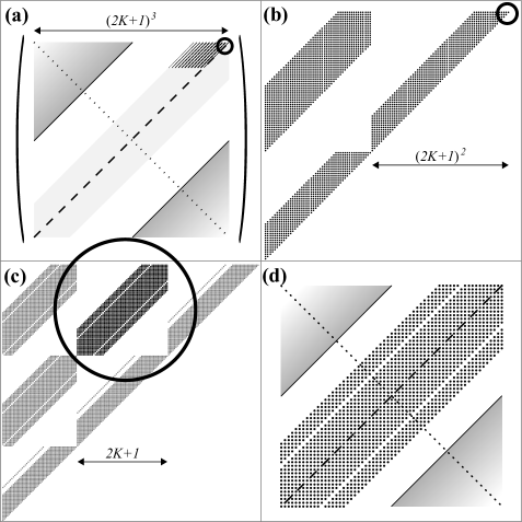
Figure 1: Illustration of the $D$-block-Hankel structure for the actual $A_{12}$ block-matrix used in the numerical example with $D=3$ and $K=30$ reported in this section. Figure (a) illustrates the entire $226981\times 226981$ $A_{12}$ matrix, while (b), (c) and (d) shows zoomed in regions corresponding to the circle of the previous subfigure. Note that in (b) each dot represents a $2$-block-Hankel matrix, while in (c) and (d) each dot represent a single non-zero matrix element. Dashed (dotted) lines in (a) shows the skew-diagonal (diagonal) which corresponds to the skew-diagonal transpose (SDT) (respectivelly SDH for complex matrix elements) and transpose symmetries discussed in section 3.3.1. However, let us stress that the symmetry of a $D$-block-Hankel matrix is considerable higher, since the block-matrices in (a) and (b) [elements in (d)] are repeated downwards parallell to the respective skew-diagonals. Grey triangular regions in (a) and (d) shows where the conditions $\left|n_{j}^{R}+n_{j}^{C}\right|>K$ for $j=3$ respectivelly $j=1$ are fulfilled. As discussed in section 3.3.1, these regions does not contain any non-zero matrix elements due to the restricted Fourier coefficients lattice size. The fact that the regions of non-zero elements do not reach out to the grey fields are due to the truncation implemented, see text for details.

6.1 Physical parameters

In order to use a realistic set of parameters for our numerical example, we chose an harmonic trap with frequences such that the size of the molecular field along the $x$-direction $R_{TF,x}=8\,\mu$m is two times the size along the $z$-direction $R_{TF,z}=4\,\mu$m, while the size along the $y$-direction $R_{TF,y}=6\,\mu$m is set to an intermediate value. With a central molecular peak density of $\rho_{0}=10^{20}$m^-3, this corresponds to $N_{0}\simeq\frac{8\pi}{15}\rho_{0}R_{TF,x}R_{TF,y}R_{TF,z}\simeq 3.2\cdot 10^{4}$ molecules. Choosing ${}^{40}K_{2}$ dimers [13] we have an atomic mass of $m_{at}=6.642\cdot 10^{-26}$kg. The molecule-atom dissociation parameter is $\chi=10^{-7}$m^3/2/s here [28]. We set the dissociation detuning to $\Omega=-4\cdot 10^{3}$s^-1 which is large enough to ensure that the dissociation energy is larger than thermal excitations at nK temperatures (i.e. $2\hbar\left|\Omega\right|\gg k_{B}T$). With a characteristic time of $t_{0}=1$ms this corresponds to a dimensionless detuning of $\delta=t_{0}\Omega=-4$ [28]. The momentum lattice in use have a spacing $dk\equiv dk_{x}=dk_{y}=dk_{z}\simeq 1.1\cdot 10^{5}$m^-1 which is smaller than the smallest width of the molecular momentum distribution $\sim 2/R_{TF,x}$ [23], and have been confirmed numerically to resolve the dynamics of the relevant structures in the atomic momentum distribution. The corresponding resonance momenta is then $k_{0}=\left|\mathbf{k}_{0}\right|=\sqrt{2m_{at}\left|\Omega\right|/\hbar}\simeq 20dk$.

6.1.1 Fermi’s Golden Rule estimate of the atom numbers

For small times we can, for the purpose of validating the physical parameters, estimate the number of atoms by the following linear expression in time

$$N_{j}\left(t\right)\simeq N_{0}\lambda t,\>\>\lambda=\frac{1}{\sqrt{2}\pi}\left(\frac{m_{at}}{\hbar}\right)^{3/2}\chi^{2}\sqrt{\left|\Omega\right|}.$$ (70)

From the above formula it is clear that the number of atoms increase with $\left|\Omega\right|$ for a three-dimensional system. This have earlier been studied explicitly for a uniform system, see Fig. 1 of [28]. Hence for cases with large detuning the validity of the undepleted field approximation is limited to short dissociation times $t/t_{0}\ll 1$. For the parameters of section 6.1 we have $\lambda\sim 2s^{-1}$ which results in $N_{j}\sim 10^{2}$ atoms at $t=t_{0}$, and hence a conversion ratio of less than 1%, ensuring the validity of the results from the undepleted field approximation [23, 25, 26]. The presented estimate of atom numbers from the Fermi’s Golden Rule (70) was later confirmed by the numerical calculations for the parameter values in use here.

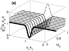
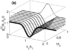
Figure 2: Fermionic collinear atom-atom correlation functions in momentum space $g_{11}^{(2)}(\mathbf{k},\mathbf{k}^{\prime},t)$, at times $t/t_{0}=0.1,\>0.2,\>...,\>1$ ($t_{0}=1$ms), calculated along different directions in 3D. In (a) we show numerical results (solid thin curves) from (67) along the direction $\mathbf{e}_{x}$, i.e. with $\mathbf{k}=k_{x}\mathbf{e}_{x}$ and $\mathbf{k}^{\prime}=k_{0}\mathbf{e}_{x}$ ($k_{0}\simeq 2.2\cdot 10^{6}$m^-1), while in (b) we show the corresponding result along the direction $\mathbf{e}_{z}$. The analytic short-time asymptotes of (71) are represented by the fat curves plotted at $t/t_{0}=0.1$ only. In fact the short-time asymptotes for the collinear correlations are in qualitative agreement with the numerical results even up to $t/t_{0}\sim 1$. However, a zoom in reveals quantitative deviations seen as a narrowing of the width of the correlation signal with time, this is also in agreement with detailed 1D results reported in Fig. 8 of [23]. In general the fermionic collinear correlations are here showing a Pauli-blocking dip at $k_{x,z}=k_{0}$, while the characteristic width of the correlation signal have been confirmed to be inverselly proportional to the size of the molecular BEC source along the corresponding direction, i.e. $\sim 2.16R_{TF,x}^{-1}\simeq 2.7\cdot 10^{5}$m^-1 in (a) and $\sim 2.16R_{TF,z}^{-1}=2\cdot 2.16R_{TF,x}^{-1}$ in (b). In addition we compared with the corresponding results for bosonic atoms showing a so called Hanbury-Brown and Twiss peak at $k_{x,z}=k_{0}$ (dashed curves), shown only for the largest time here.

6.2 Structures in the system matrix

We here explicitly illustrate the $D$-block-Hankel matrix $A_{12}$ that is used in the numerical calculations of a physical system for $D=3$ here. Hence, it is evident from the figures 1 (a), (b) and (c) that we can zoom in $D=3$ times on $A_{12}$ and reveal a repeating pattern. Clearly after the last zoom in [figure 1 (d)], we are left with a structure of a usual Hankel matrix.

We have used a truncation of the molecular BEC source such that Fourier coefficients with a modulus less than 2% of the leading coefficient is neglected. This procedure have been evaluated by reconstruction of the BEC by the inverse Fourier transform. It was also found that the 2% level of truncation resulted in correlation functions (see figure 2) that could not be distingushable by the eye from the correlation functions obtained with a 4% level of truncation.

6.3 Numerical comparison with analytic asymptotes

For $D=3$ the Thomas-Fermi (TF) density profile of the molcular BEC is given by $\rho_{0}(\mathbf{x})=\rho_{0}(1-x^{2}/R_{\mathrm{TF},x}^{2}-y^{2}/R_{\mathrm{TF},y}^{2}-z^{2}/R_{\mathrm{TF},z}^{2})$ for $x^{2}/R_{\mathrm{TF},x}^{2}+y^{2}/R_{\mathrm{TF},y}^{2}+z^{2}/R_{\mathrm{TF},z}^{2}<1$ [and $\rho_{0}(\mathbf{x})=0$ otherwise], which is underlying an analytic derivation of the asymptotes. Here $R_{\mathrm{TF},j}$ is the Thomas-Fermi radius along the spatial direction $j=x,y,z$. We are here interested in collinear (CL) density correlations between two momentum components at $\mathbf{k}$ and $\mathbf{k}^{\prime}$, for which the displacement $\Delta\mathbf{k=k-k}^{\prime}$ is along one of the Cartesian coordinates, $k_{j}$. The detailed derivation of short-time asymptotes for the correlation functions in this case was reported in [23]. The CL correlations following from this derivation is

$$g_{11}^{(2)}(k_{j},k_{j}^{\prime},t)\simeq 1+q\frac{225\pi}{2}\frac{\left[J_{5/2}\left((k_{j}-k_{j}^{\prime})R_{\mathrm{TF},j}\right)\right]^{2}}{\left[(k_{j}-k_{j}^{\prime})R_{\mathrm{TF},j}\right]^{5}},$$ (71)

where $J_{\nu}$ denotes Bessel functions of the first kind. The qualitative behavior of the CL correlation functions are similar as in lower dimensions [34, 46], whereas the quantitative differences enter e.g. through the width and the peak values. The widths of (71) is $w_{i}^{\left(CL\right)}\simeq 2.16/R_{TF,j}$ and the peak value of (71) is static to leading order [23].

In figure 2 we show results for the evaluation of the analytic short-time asymptote (71), strictly valid in the $t/t_{0}\ll 1$ limit, against numerical results for times $t/t_{0}\leq 1$, where $t=t_{0}$ roughly corresponds to the first maximum in time of the oscillating fermionic atom numbers $N\left(t\right)=\sum_{\mathbf{k},\sigma}n_{\mathbf{k},\sigma}\left(t\right)$.

7 Summary

We have described how to effectivelly calculate the dynamics of linear Heisenberg operator equations for the Fermi-Bose model applied to the problem of molecular dissociation. We note that a similar framework have been used to obtain numerical results for a non-isotropic 2D system on a $61\times 61$ grid in [34]. We have here generalized the approch to $D$ spatial dimensions with the use of $D$-block-Hankel matrices. In particular we have explicitly explored a non-isotropic 3D system on a $61\times 61\times 61$ grid numerically on a standard PC. Such a grid can resolve relevant atom dynamics in momentum space for realistic parameters [9], and naturally extends earlier studies of non-uniform 1D and 2D systems [34, 46], and is more realistic than previous treatments of uniform 3D systems [9, 28]. We finally stress that the results presented can be used to handle a complex bosonic mean-field of any geometry in any spatial dimension.

References

• [1] Friedberg R and Lee T D 1989 Phys. Rev. B 40, 6745.
• [2] Kheruntsyan K V and Drummond P D 2000 Phys. Rev. A 61, 063816.
• [3] Holland M, Kokkelmans S J J M F, Chiofalo M L and Walser R 2001 Phys. Rev. Lett. 87, 120406.
• [4] Timmermans E, Furuya K, Milonni P W and Kerman A K 2001 Phys. Lett. A 285, 228.
• [5] Ohashi Y and Grin A 2002 Phys. Rev. Lett. 89, 130402.
• [6] Strohmaier N, Greif D, Jördens R, Tarruell L, Moritz H, Esslinger T, Sensarma R, Pekker D, Altman E and Demler E 2010 Phys. Rev. Lett. 104, 080401.
• [7] Jördens R, Strohmaier N, Gunter K, Moritz H and Esslinger T 2008 Nature (London) 455, 204.
• [8] Jack M W and Pu H 2005 Phys. Rev. A 72, 063625.
• [9] Kheruntsyan K V 2006 Phys. Rev. Lett. 96, 110401.
• [10] Mukaiyama T, Abo-Shaeer J R, Xu K, Chin J K and Ketterle W 2004 Phys. Rev. Lett. 92, 180402.
• [11] Dürr S, Volz T and Rempe G 2004 Phys. Rev. A 70, 031601(R).
• [12] Thompson S T, Hodby E, Wieman C E 2005 Phys. Rev. Lett. 94, 020401.
• [13] Greiner M, Regal C A, Stewart J T and Jin D S 2005 Phys. Rev. Lett. 94, 110401.
• [14] Lee T D 1954 Phys. Rev. 95, 1329.
• [15] Källén G and Pauli W 1955 Kgl. Danske Vidensk. Selsk. Mat.-Fys. Medd. 30 No. 7.
• [16] Heisenberg W 1957 Nuclear Physics 4, 532.
• [17] Poulsen U V and Mølmer K 2001 Phys. Rev. A 63, 023604.
• [18] Drummond P D and Kheruntsyan K V 2002 Phys. Rev. A 66, 031602(R).
• [19] Cazalilla M A and Marston J B 2002 Phys. Rev. Lett. 88, 256403.
• [20] Schollwöck U 2011 Annals of Physics 326, 96.
• [21] Deuar P, Chwedeńczuk J, Trippenbach M and Ziń P 2011 Phys. Rev. A 83, 063625.
• [22] Krachmalnicoff V, Jaskula J-C, Bonneau M, Leung V, Partridge G B, Boiron D, Westbrook C I, Deuar P, Ziń P, Trippenbach M and Kheruntsyan K V 2010 Phys. Rev. Lett. 104, 150402.
• [23] Ögren M and Kheruntsyan K V 2010 Phys. Rev. A 82, 013641.
• [24] Savage C M, Schwenn P E and Kheruntsyan K V 2006 Phys. Rev. A 74, 033620.
• [25] Midgley S L W, Wüster S, Olsen M K, Davis M J, and Kheruntsyan K V 2009 Phys. Rev. A 79, 053632.
• [26] Ögren M, Kheruntsyan K V and Corney J F 2010 Europhys. Lett., 92 36003.
• [27] Ögren M, Kheruntsyan K V and Corney J F 2011 Comput. Phys. Commun. 182, 1999.
• [28] Davis M J, Thwaite S J, Olsen M K and Kheruntsyan K V 2008 Phys. Rev. A 77, 023617.
• [29] Corney J F and Drummond P D 2004 Phys. Rev. Lett. 93, 260401.
• [30] Corney J F and Drummond P D 2006 J. Phys. A: Math. Gen. 39, 269.
• [31] Rahav S and Mukamel S 2009 Phys. Rev. B 79, 165103.
• [32] Rosales-Zárate L E C and Drummond P D 2011 Phys. Rev. A 84, 042114.
• [33] Fetter A L and Walecka J D 2003 Quantum Theory of Many-Particle Systems, Dover.
• [34] Ögren M, Savage C M, and Kheruntsyan K V 2009 Phys. Rev. A 79, 043624.
• [35] Deuar P, Ziń P, Chwedeńczuk J, Trippenbach M 2011 Eur. Phys. J. D 65, 19.
• [36] Poulsen U V and Mølmer K 2007 Phys. Rev. A 76, 013614.
• [37] Castin Y and Dum R 1996 Phys. Rev. Lett. 77, 5315.
• [38] Ziń P, Chwedeńczuk J, Trippenbach M 2006 Phys. Rev. A 73, 033602.
• [39] Ögren M and Kheruntsyan K V 2009 Phys. Rev. A 79, 021606(R).
• [40] Ögren M and Kheruntsyan K V 2007 unpublished.
• [41] Peller V 2003 Hankel operators and their applications, Springer-Verlag N. Y.
• [42] Andersson F, Carlsson M and de Hoop M V 2010 Appl. Comput. Harmon. Anal. 29, 156.
• [43] Lang S 1999 Complex Analysis, 4.th ed. Springer-Verlag N. Y., Grad. Texts in Math. 103.
• [44] Moler C and Van Loan C 2003 SIAM Rev. 45 3.
• [45] Sidje R B 1998 ACM Trans. Math. Softw., 24(1):130-156.
• [46] Ögren M and Kheruntsyan K V 2008 Phys. Rev. A 78, 011602(R).