Elastic enhancement factor as a quantum chaos probe

Abstract

Recent development of the resonance scattering theory with a transient from the regular to chaotic internal dynamics inspires renewed interest to the problem of the elastic enhancement phenomenon. We reexamine the question what the experimentally observed value of the elastic enhancement factor can tell us about the character of dynamics of the intermediate system. Noting first a remarkable connection of this factor with the time delays variance in the case of the standard Gaussian ensembles we then prove the universal nature of such a relation. This reduces our problem to that of calculation of the Dyson’s binary form factor in the whole transition region. By the example of systems with no time-reversal symmetry we then demonstrate that the enhancement can serve as a measure of the degree of internal chaos.

Excess of probabilities of elastic processes over inelastic ones is a common feature of the resonance compound nuclear reactions, electron transport through quantum dots, where it manifests itself as the weak localization effect, or, at last, transmission of electromagnetic waves through microwave cavities. This phenomenon, that is characterized quantitatively by the elastic enhancement factor i.e. the typical ratio $F$ of elastic and inelastic cross sections, repeatedly attracted attention for decades Collection ; Lewenkopf ; Pluhar ; Verbaarshot ; Fyodorov . Based on the random matrix theory Mehta universal formalism that allows of uniform treatment of all resonance phenomena of such a kind has been worked out in the seminal paper Zirnbauer . The scattering $M\times M$ matrix that describes the resonance processes is expressed as

$$S(E)=I-iA^{{\dagger}}\frac{1}{E-H+\frac{i}{2}A\,A^{{\dagger}}}\,A\,.$$ (1)

The Hamiltonian matrix $H$ that describes dynamics of the originally closed intermediate system is supposed to belong to an ensemble of random matrices. This system gets excited and then decays after a while because its $N\gg 1$ eigenstates are connected to $M$ open channels via random Lehmann rectangular $N\times M$ matrix $A$. The formula (1) can be naturally interpreted Rotter ; Sokolov (see also Sommers ; Mitchell and references therein) within the concept of open systems whose internal dynamics is described by a non-Hermitian effective Hamiltonian $\mathcal{H}=H-\frac{i}{2}W$ where the connection to channels results in the anti-Hermitian contribution proportional to the matrix $W=A\,A^{{\dagger}}$. The complex eigenvalues of the effective Hamiltonian specify positions and widths of the resonances.

All quantities of the physical meaning are obtained by averaging $\langle...\rangle$ over two independent ensembles of matrices $H$ and $A$ Lehmann . Specifically, the averaged scattering matrix $\langle S^{ab}(E)\rangle=\langle S^{aa}(E)\rangle\,\delta^{ab}$ fixes the transmission coefficients $T^{a}=1-|\langle S^{aa}\rangle|^{2}$ that measure the part of the flow that spends essential time in the internal region. The scale of the energy dependence of the mean scattering matrix as well as the transmission coefficients is large and their energy variations can be neglected within the energy interval where the $N$ resonance states of interest are situated.

In the most interesting case of large number $M\gg 1$ of scattering channels (for the sake of simplicity we suppose that all these channels are statistically equivalent and have, therefore, identical transmission coefficients $T$) the enhancement factor $F$ consists of two contributions of quite different nature. The first of them, $1+\delta_{1\beta}$, depends only on the symmetry class $\beta=1$ (preserved time-reversal (T) invariance) or $\beta=2$ (broken T-invariance) of the corresponding ensembles of the random effective Hamiltonians ${\cal H}$ Lewenkopf ; Lehmann ; Pluhar . No enhancement originates from this contribution in the case of Unitary ensemble of complex Hermitian matrices. The second contribution is regulated by the ratio $\eta=t_{H}/t_{W}=MT$ (”openness”) of two characteristic times. One of them, the Heisenberg time

$$t_{H}=\frac{2\pi}{d}=-2\Im\left\langle\mathrm{Tr}\,G(E+i0)\right\rangle\,,$$ (2)

where $G(E+i0)=\left(E+i0-H\right)^{-1}$ is the resolvent of the Hamiltonian $H$, characterizes the internal motion and is defined by its mean level spacing $d$. Similarly Dittes ; Savin , the dwell time $t_{W}=\frac{1}{T}\langle Q\rangle_{A\rightarrow\,0}$, where $\langle Q\rangle=-\frac{2}{M}\Im\langle\mathrm{Tr}\frac{1}{E-\mathcal{H}}\rangle$ is the mean delay time, establishes the time scale of the open system in terms of the mean Wigner delay time Wigner ; Smith . The dwell time is the time the incoming particle spends in the internal region. The inverse quantity $\Gamma_{W}=1/t_{W}$ is nothing else than the well-known Weisskopf width Weisskopf . Only if the openness is small enough, $\eta\ll 1$, so that the dwell time appreciably exceeds the Heisenberg time, $t_{H}\ll t_{W}\,$, the incoming particle has enough time to recognize the discreteness of the internal spectrum and therefore to perceive spectral fluctuations. Then an additional contribution appears Verbaarshot ; Fyodorov and the enhancement factor takes finally the form

$$F^{(\beta)}(\eta)=1+\delta_{\beta 1}+\eta\,\int_{0}^{\infty}dse^{-\eta s}\,\left[1-B_{2}^{(\beta)}(s)\right]\,\\$$ (3)

where $B_{2}^{(\beta)}(s)$ is the Dyson’s spectral binary form factor Mehta belonging to the symmetry class $\beta$. Comparing this expression with the delay time two-point correlation function

$$\begin{array}[]{c}K^{(\beta)}(\epsilon)=\frac{\langle Q(\frac{\epsilon}{2})Q(-\frac{\epsilon}{2})\rangle}{\langle Q^{2}\rangle}-1\\ =\int_{0}^{\infty}ds\,e^{-\eta s}\left[1-B^{(\beta)}_{2}(s)\right]\cos\left(2\pi s\rho\epsilon\right)\\ \end{array}$$ (4)

calculated for the case $\beta=1$ in Savin (later on, similar calculation has been performed also in the case $\beta=2$ Fyodorov+ ) we arrive at the following remarkable relation between the enhancement factor and variance of the time delays:

$$\begin{array}[]{c}F^{(\beta)}(\eta)=1+\delta_{\beta 1}+\eta\,varQ(\eta)\\ =2+\delta_{\beta 1}-\eta\,\int_{0}^{\infty}ds\,e^{-\eta s}\,B_{2}^{(\beta)}(s)\,.\end{array}$$ (5)

A new aspect of the old problem of the elastic enhancement has been recently evoked in ref.Celardo (see also earlier semiclassical consideration in Baranger ) where manifestations of transition from regular to chaotic internal motion has been investigated in the framework of the resonance scattering theory. The character of this motion is controlled by a particle interaction parameter $\kappa$. The dynamics of the intermediate system can therefore be described by some transient matrix ensemble. It has been, in particular, numerically discovered that the elastic enhancement factor is quite sensitive to the strength of the interaction. This fact suggests that the enhancement factor can serve as an indicator of the degree of the internal chaoticity. In what follows we investigate this relation analytically.

Generally, the short range universal fluctuations of scattering amplitudes are described by the (connected) $S$-matrix two-point auto-correlation function Zirnbauer

$$C^{abcd}(\epsilon)=\langle S^{ab}(E+\epsilon/2)S^{cd\,*}(E-\epsilon/2)\rangle_{conn}\,.$$ (6)

While carrying out the ensemble averaging we, suppose throughout this Letter the decay amplitudes $A_{n}^{c}$ to be uncorrelated Gaussian random quantities

$$\langle A_{n}^{a}A_{m}^{b\,*}\rangle_{A}=\frac{\gamma}{N}\delta_{nm}\delta^{ab}\,.$$ (7)

This assumption is supported by the reasons of so-called ”geometrical chaos” that have been argued in ref. Zelevinsky . In the case of T-invariant systems $\beta=1$ these amplitudes are real, $A_{m}^{b\,*}=A_{m}^{b}$.

For the elastic enhancement factor the formula (6) gives $F=C^{aaaa}(0)/C^{abab}(0)\,$. We start ensemble averaging with that over the amplitudes $A$ keeping the internal Hamiltonian $H$ diagonal. It is convenient (though not necessary) to use supersymmetric integral representation. Then $A$-averaging can be fulfilled exactly whereupon the saddle point method can be used. In such a way we receive first of all

$$\langle S^{ab}(E)\rangle=\delta^{ab}\left\langle\frac{1-i\frac{\gamma}{2}g(E)}{1+i\frac{\gamma}{2}g(E)}\right\rangle_{P}\,,$$ (8)

where the function $g(E)\equiv\frac{1}{N}\langle\mathrm{Tr\frac{1}{E-{\cal H}}}\rangle_{A}$ satisfies the equation (m=M/N)

$$g(E)=\frac{1}{N}\sum_{n=1}^{N}\left[E-E_{n}+\frac{\frac{i}{2}m\gamma}{1+\frac{i}{2}\gamma g(E)}\right]^{-1}\,.$$ (9)

The subscript $P$ in the r.h.s. of eq. (8) implies averaging over all energy levels of the internal system with the joint probability distribution $P(\{E\}|\kappa)$; $\{E\}\equiv E_{1},E_{2},...E_{N}$ at a given value of the chaoticity parameter $\kappa$. Depending on this parameter, the distribution $P(\{E\}|\kappa)$ changes from Poissonian distribution of fully independent levels ($\kappa=0$) to that of highly correlated levels what is typical of the Gaussian ensembles ($\kappa=\infty$). We assume also that the mean level density does not depend on $\kappa$ at all.

In the limit of weak coupling to continuum $\gamma\rightarrow 0$ we are interested in, the approximate solution of eq. (9) reads

$$g(E)\approx\frac{1}{N}\mathrm{Tr}\,G\left(E+\frac{i}{2}m\gamma\right)\,.$$ (10)

We suppose below that the ratio $m$ is also small. Then the mean scattering matrix reduces Sokolov ; Sokolov+ to

$$\langle S^{ab}(E)\rangle=\delta^{ab}\frac{1-i\frac{\gamma}{2}\left\langle g(E)\right\rangle_{P}}{1+i\frac{\gamma}{2}\left\langle g(E)\right\rangle_{P}}=\frac{1-x}{1+x}\,.$$ (11)

In accordance with the conventional practice, we neglected the long range energy dependence of the mean $S$-matrix elements and set $E=0$. (We will do the same in all later calculations.) The measuring the degree of resonance overlapping parameter $x=\frac{\pi\gamma}{2N\,d}$ (where $d$ is the mean level spacing) should be small in the case of our interest so that the corresponding transmission coefficients equal $T\approx 4\,x$ and, correspondingly, the openness is $\eta=4M\,x=2\pi m\frac{\gamma}{d}\,$.

The tensor structure of the correlation function $(\ref{S-S})$

$$C^{abcd}(\epsilon)=F_{1}^{(\beta)}(\epsilon)\delta^{ab}\delta^{cd}+F_{2}^{(\beta)}(\epsilon)(\delta^{ac}\delta^{bd}+\delta_{1\beta}\delta^{ad}\delta^{bc})\,$$ (12)

follows from the T-invariance properties and rotational invariance in the channel space. The superscript $\beta$ marks now the symmetry class of the limiting ($\kappa=\infty$) matrix ensemble. The enhancement factor reads therefore

$$F^{(\beta)}=1+\delta_{\beta 1}+\left[F_{1}^{(\beta)}(\epsilon)\Big{/}F_{2}^{(\beta)}(\epsilon)\right]_{\epsilon=0}\,.$$ (13)

Now, in the leading order with respect to $\gamma$ the $A$-averaging results in

$$\begin{array}[]{l}F_{1}^{(\beta)}(N,M,\gamma|\kappa)=\frac{\gamma^{2}}{N^{2}}\left\langle\mathrm{Tr}\,G(\frac{i}{2}m\gamma)\mathrm{Tr}\,G^{\dagger}(\frac{i}{2}m\gamma)\right\rangle_{P,\,conn}\\ F_{2}^{(\beta)}(N,M,\gamma|\kappa)=\frac{\gamma^{2}}{N^{2}}\left\langle\mathrm{Tr}\,G(\frac{i}{2}m\gamma)G^{\dagger}(\frac{i}{2}m\gamma)\right\rangle_{P}\,.\end{array}$$

Subsequent $P$-averaging is straightforward and leads to the expression

$$F_{1}^{(\beta)}\Big{/}F_{2}^{(\beta)}=\eta\int_{0}^{\infty}ds\,e^{-\eta s}\left[1-B_{2}^{(\beta)}(s|\kappa)\right]\,.$$ (14)

Note that this ratio depends after all only on two parameters: on the openness $\eta$ of the internal system and on the degree of chaoticity $\kappa$ of its dynamics. Finally, we arrive at the expression

$$F^{(\beta)}(\eta|\kappa)=2+\delta_{\beta 1}-\eta\int_{0}^{\infty}ds\,e^{-\eta s}B_{2}^{(\beta)}(s|\kappa)$$ (15)

that extends the relations (3, 5)) to the case of arbitrary value of the chaoticity parameter.

The found result reduces the problem posed above to that of calculating the binary form factor $B_{2}^{(\beta)}(s|\kappa)$ in the whole transient region $0\leqslant\kappa<\infty$. The issue of transition from regular to chaotic dynamics has been attacked not once by different authors (see Guhr98 and references therein). The total solution has been found by now only in the case of the systems with broken time-reversal symmetry Pandey ; Shapiro . The method used in Shapiro is the most convenient for our purpose. These authors has used the Brezin-Hikami’s approach Brezin96 that allows of direct calculating the binary form factor we need. Below we restrict ourselves to the case $\beta=2$ and will skip this superscript.

The following two properties of the considered binary form factor are obvious from the very beginning: $B_{2}(s|0)=0$ and $B_{2}(s|\infty)=(1-s)\theta(1-s)$, Mehta . In the intermediate region the form factor is given by Shapiro

$$\begin{array}[]{l}B_{2}(s|\kappa)=B_{2}(s|\infty)\\ -\frac{2}{\pi}\int_{-1}^{1}dy\frac{[2y\sqrt{s}+1]\sqrt{1-y^{2}}}{s+2y\sqrt{s}+1}e^{-\kappa s(s+2y\sqrt{s}+1)}\,.\end{array}$$ (16)

In fact, only the even part of the integrand contributes. The enhancement factor is entirely expressed via the function

$$\begin{array}[]{c}\Psi(\eta|\kappa)=\eta\int_{0}^{\infty}ds\,e^{-\kappa\,s(s+1)-s\eta}\,\,\frac{I_{1}(2\kappa\,s^{3/2})}{\kappa\,s^{3/2}}\\ =\eta\int_{0}^{\infty}ds\,e^{-\kappa\,s(s+1)+2\kappa\,s^{3/2}-s\eta}\,\Xi(2\kappa\,s^{3/2})\\ \end{array}$$ (17)

where $I_{1}(x)$ stands for the modified Bessel function and the function $\Xi(2\kappa\,s^{3/2})=e^{-2\kappa\,s^{3/2}}\frac{I_{1}(2\kappa\,s^{3/2})}{\kappa\,s^{3/2}}$ decreases monotonously from one to zero when the argument $2\kappa\,s^{3/2}$ grows. It is easy to check that $\Psi(\eta|0)=1$, $\,\Psi(\eta|\infty)=0$ and $\Psi(\eta|\kappa)>0$ in between.

There are two equivalent representations of the enhancement factor:

$$F(\eta|\kappa)=1+\Psi(\eta|\kappa)+\eta\frac{\partial^{2}}{\partial\eta^{2}}\left[\frac{1}{\eta}\int_{0}^{\kappa}d\kappa^{\prime}\Psi(\eta|\kappa^{\prime})\right]\,,$$ (18)

and

$$\begin{array}[]{c}F(\eta|\kappa)=1+(1-e^{-\eta})\left/\eta\right.\\ \\ +\Psi(\eta|\kappa)-\eta\frac{\partial^{2}}{\partial\eta^{2}}\left[\frac{1}{\eta}\int_{\kappa}^{\infty}d\kappa^{\prime}\Psi(\eta|\kappa^{\prime})\right]\,.\end{array}$$ (19)

In particular, the first formula gives immediately $F(\eta|0)\equiv 2$ when the second one reduces to the GUE result $F_{GUE}=1+(1-e^{-\eta})/\eta\approx 2-\frac{1}{2}\eta+...\,$. More than that, it can be shown with the aid of eq. (19) that the slope at the point $\eta=0$ is universal:

$$\frac{\partial F(\eta|\kappa\neq 0)}{\partial\eta}\Big{|}_{\eta=0}\equiv-\frac{1}{2}\,.$$ (20)

Indeed, at any nonzero $\kappa$ contributions of the two last terms cancel each other when $\eta\rightarrow 0$ with accuracy better than $\eta$.

Although one cannot obtain any exact explicit analytical formula, a number of approximate expressions can be derived from eqs. (18, 19). At that eq.(18) is useful when the internal chaoticity is weak whereas the second form is more convenient if the internal dynamics is close to chaotic. Behavior of the function $\Psi$ depends on interrelation of the two competing parameters $\kappa$ and $\eta$. If the first of them is small enough and the second one is kept finite we can take into account only few leading terms in the Bessel function power series. Corresponding contributions are expressed already in the terms of known transcendental functions. After that there are two possibilities: either expand these functions into power series with respect to the parameter $\kappa$ or make expansion over inverse powers of the parameter $\eta$. In the first case coefficients of the $\kappa$-expansion are polynomials in $1/\eta$; in the second case those of the $1/\eta$-expansion are polynomials in $\kappa$. The two found in such a way expansions do not perfectly coincide. Nevertheless they match with certain accuracy that can be improved by taking into account a larger number of contributions. Substituting finally the estimated in such a way function $\Psi$ into eq. (18) we arrive at

$$F(\eta|\kappa)=2-\frac{\kappa}{\eta}+\frac{(6+\eta)\kappa^{2}}{\eta^{3}}-\frac{(60+\eta(20+\eta))\kappa^{3}}{\eta^{5}}+...\,.$$ (21)

On the other hand, if the parameter of chaoticity is large, $\kappa\gg 1$, calculations become appreciably simpler and integration in eq. (17) can be carried out with the help of the Laplace method. At that, it is convenient to utilize the presentation given in the second line of eq. (17). Generally speaking, the exponential factor in the integrand has two maxima in the points $s_{0}=0$ and $s_{1}=1/8\left(5-4\eta/\kappa+3\sqrt{1-8\eta/\kappa}\right)\,.$ In the first of them the whole integrand equals one. Then $\Psi(\eta|\kappa)\approx\frac{\eta}{\eta+\kappa}$ and the contribution of the vicinity of the point $s_{0}$ in the enhancement factor is easily found to be

$$F(\eta|\kappa)\approx 1+\frac{1-e^{-\eta}}{\eta}+\frac{\eta}{\eta+\kappa}-\frac{\eta}{(\eta+\kappa)^{2}}\,.$$ (22)

As to the second point $s_{1}$, the maximum of the exponential reaches its largest possible value one when $\eta=0$, goes rapidly down with growing $\eta$ and, after passing the inflection point $s_{i}=9/16$, disappears finally when $\eta$ exceeds $\kappa/8\,.$ But even in the most interesting case $\kappa\gg\eta\gtrsim 1$ contribution of the vicinity of the second maximum remains negligible. Indeed, opposite to the hight of the maximum neither its position $s_{1}\approx 1$, nor its width $\Delta s\approx 0.4$ noticeably depend on $\eta\,.$ Therefore the slow varying factor can be estimated as $\Xi(2\kappa s^{3/2})\approx\Xi(2\kappa s_{1}^{3/2})\approx 1\left/\sqrt{2\pi}\,\kappa^{3/2}\right.\ll 1\,.$

The Fig.1 illustrates variations of the elastic enhancement factor depending on the increasing openness $\eta$ and parameter chaoticity $\kappa$. In particular, the domains of validity of our approximations are demonstrated. At any given chaoticity $\kappa$ the factor $F(\eta|\kappa)$ decreases with the universal initial slope $-1/2$ starting from the maximal value 2 up to some value $\eta_{c}(\kappa)$ where this factor reaches minimum $F_{min}$ so that

$$\frac{\partial F(\eta|\kappa)}{\partial\eta}\Big{|}_{\eta=\eta_{c}(\kappa)}=0.$$ (23)

The level correlations at the chosen value of the chaoticity parameter $\kappa$ are too weak to be resolved when openness $\eta$ exceeds the value $\eta_{c}(\kappa)$ and the enhancement factor returns to value 2 typical of the system with regular dynamics. In this way the enhancement factor conveys information on the degree of internal chaos. Finally, the required chaoticity parameter $\kappa(F_{min})$ is found as the root of the equation $F\left(\eta_{c}(\kappa)|\kappa\right)=F_{min}\,.$

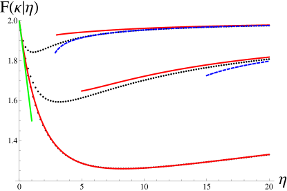
Figure 1: (color online) Enhancement factor $F(\eta|\kappa)$ as a function of $\eta$ for three fixed values (from top to bottom) $\kappa=(0.5,5,50)$. Black points - exact numerical results, blue lines (dashed) - small $\kappa$ approximation (21), red lines (full) - large $\kappa$ approximation (22); the straight green (gray) line shows the universal slope at the point $\eta=0$.

Though we do not know the explicit form of the binary form factor $B^{(\beta=1)}_{2}(s|\kappa)$ that describes considered transition in the case of $T$-invariant systems, there is no doubt that, qualitatively, the behavior of the enhancement factor should be similar. It is worth mentioning that the evolution of this factor under transition from perfectly chaotic systems with broken $T$-invariance to $T$-invariant ones can easily be followed with the aid of the method developed in Fyodorov++ .

The further quite nontrivial development reported in Brezin03 opens opportunity of deriving such a form factor for T-invariant systems also. Corresponding results will be published elsewhere.

Summary We have considered the dependence of the elastic enhancement factor on the degree of chaoticity of the internal part of an open resonance system. A general relation of this factor with the variance of time delays has been established for arbitrary degree of chaoticity. By this, the task is reduced to the search for the transient binary form factor. Generally, the enhancement factor $F(\eta|\kappa)$ depends on both the chaoticity parameter $\kappa$ and the openness $\eta$ the latter being the ratio $\eta=t_{H}/t_{W}$ of two characteristic times: the dwell time $t_{W}$ and the Heisenberg time $t_{H}$. Here the time $t_{H}=\frac{2\pi}{d}$ is the time that is needed to resolve the pattern of spectral fluctuations in the system with Hamiltonian $H$ when the time $t_{W}=1/\Gamma_{W}$ is that the incoming particle spends in average inside this system. Only if this particle is trapped inside for sufficiently long time it can carry information on the internal chaos. Otherwise the difference between regular and chaotic internal dynamics cannot be resolved.

In this Letter, the problem posed has been thoroughly studied numerically and analytically in the case of systems with no time-reversal symmetry. We showed in particular that the slope $\frac{\partial F(\eta|\kappa\neq 0)}{\partial\eta}\Big{|}_{\eta=0}=-\frac{1}{2}$ remains invariable for arbitrary degree of internal chaos. The recovery of the maximal value of $F(\eta|\kappa)$ when the openness $\eta$ exceeds some value $\eta_{c}(\kappa)$ that is clearly seen in the Fig.1 is in perfect agreement with the physical argumentation stated in the previous paragraph.

We are very grateful to V.G. Zelevinsky and V.F. Dmitriev for useful discussions. This work is supported by the Ministry of Education and Science of the Russian Federation. Y. Kharkov acknowledges financial support by the “Dynasty” foundation, by the Government of Russian Federation (grant 11.G34.31.0035), by the foundation ”Leading Scientific Schools of Russia” (grant 6885.2010.2) and the Russian Foundation for basic Research (grant 12-01-00943-a). V. Sokolov appreciates financial support from the federal program ”personnel of innovational Russia” (grant 14.740.11.0082) as well as countenance by the RAS Joint scientific program ”Nonlinear dynamics and Solitons” .

References

- (1) P.A. Moldauer, Phys. Rev. 123, 968 (1961) and Phys. Rev. B 135, 642 (1964); W. Kretschmer and M. Wanger, Phys. Rev. Lett. 41, 1224 (1978); H.M. Hofmann, T. Mertelmeier, M. Herman, J.W. Tepel, Zeitschrift für Physik A 297, 153 (1980); H.L. Harney, H.A. Weidenmüller and A. Richter, Phys. Lett. B 96, 227 (1980); A. Müller and H.L. Harney, Phys. Rev. C 35, 1228 (1986); M. Lawniczak, S. Bauch, O. Hul, and L. Sirko, Phys. Rev. E 81, 046204 (2011).
- (2) M.L. Mehta Random Matrices (3th edition), ELSEVIER Ltd., Amsterdam, Netherlands.
- (3) J.J.M. Verbaarschot, H.A. Weidenmüller, and M.R. Zirnbauer, Phys. Rep. 129, 367 (1985).
- (4) P. Kleinwächter and I. Rotter Phys. Rev. C 32, 1742 (1985).
- (5) V.V. Sokolov and V.G. Zelevinsky, Phys. Lett. B 202, 10, (1988); Nucl. Phys. A 504, 562 (1989).
- (6) Y.V. Fyodorov and H.-J. Sommers, Journ. Math. Phys. 38, 1918, (1997).
- (7) G.E. Mitchell, A. Richter, and H.A. Weidenmüller Rev. Mod. Phys. 82, 2845 (2010).
- (8) C.H. Lewenkopf and H.A. Weidenmüller, Ann. Phys. (NY) 212, 53 (1991).
- (9) N. Lehmann, D. Saher, V.V. Sokolov, H.-J. Sommers, Nucl. Phys, A 582, 223, (1995).
- (10) Z. Pluhar, H.A. Weidenmüller, J.A. Zuk, C.H. Lewenkopf, and F.J. Wegner, Ann. Phys. 243, 1 (1995).
- (11) F.M. Dittes, H.L. Harney, and A. Müller, Phys. Rev. A 45, 701 (1992); Ann. Phys. 220, 159 (1992).
- (12) N. Lehmann, D.V. Savin, V.V. Sokolov, H.-J. Sommers, Physica D 86, 572 (1995).
- (13) Y.V. Fyodorov and H.-J. Sommers, Phys. Rev. Lett. 76, 4709 (1996).
- (14) E. Wigner, Phys. Rev. 98, 145 (1955).
- (15) F.T. Smith, Phys. Rev. 118, 349; 119, 2098 (1960).
- (16) J.M. Blatt and V.F. Weisskopf, Theoretical Nuclear Physics, Springer Verlag, NY, 1979.
- (17) J.J.M. Verbaarschot, Ann. Phys. 168, 368 (1986).
- (18) Y.V. Fyodorov, D.V. Savin and H.-J. Sommers, J. Phys. A: Math. Gen. 38, 10731, (2005).
- (19) G.L. Celardo, F.M. Izrailev, V.G. Zelevinsky and G.P. Berman, Phys. Rev. E 76, 031119 (2007); S. Sorathia, F.M. Izrailev, G.L. Celardo, V.G. Zelevinsky, and G.P. Berman, EPL 88, 27003 (2009).
- (20) H.U. Baranger, R.A. Jalabert and A.D. Stone, Phys. Rev. Lett. 70, 3876 (1993);
- (21) V.G. Zelevinsky and A. Volya, Phys. Rep. 391, 311 (2004).
- (22) V.V. Sokolov and V.G. Zelevinsky, Ann. Phys. 216, 323 (1992).
- (23) T. Guhr, A. Müller-Groeling, and H. A. Weidenmüller, Phys. Rep. 299, 189 (1998).
- (24) A. Pandey, Chaos Solitons Fractals, 5, 1275 (1995); T. Guhr, Phys. Rev. Lett. 76, 1870 (1996); T. Guhr and A. Müller-Groeling, Journ. Math Phys. 38, 2258 (1997).
- (25) H. Kunz and B. Shapiro, Phys. Rev. E, 58, 400 (1998).
- (26) E. Brezin and S. Hikami, Nucl. Phys. B, 479, 697 (1996).
- (27) Y.V. Fyodorov, D.V. Savin, and H.-J. Sommers, Phys. Rev. E, 55, R4857 (1996).
- (28) E. Brezin and S. Hikami, Journ. Phys. A: Math Gen., 36, 711 (2003).