Violation of Cauchy-Schwarz inequalities by spontaneous Hawking radiation in resonant boson structures

Abstract

The violation of a classical Cauchy-Schwarz (CS) inequality is identified as an unequivocal signature of spontaneous Hawking radiation in sonic black holes. This violation can be particularly large near the peaks in the radiation spectrum emitted from a resonant boson structure forming a sonic horizon. As a function of the frequency-dependent Hawking radiation intensity, we analyze the degree of CS violation and the maximum violation temperature for a double barrier structure separating two regions of subsonic and supersonic condensate flow. We also consider the case where the resonant sonic horizon is produced by a space-dependent contact interaction. In some cases, CS violation can be observed by direct atom counting in a time-of-flight experiment. We show that near the conventional zero-frequency peak, the decisive CS violation cannot occur.

I Introduction

The emission of Hawking radiation (HR) from the horizon of a black hole (BH) is an intriguing prediction of modern physics hawking1974 . Due to the extremely low effective temperature, its detection in a cosmological context is unlikely to be achieved in the foreseeable future. However, it was noted by Unruh Unruh1976 ; Unruh1981 that HR is an essentially kinematic effect that could be observed on a laboratory scale at temperatures which, while still too low, lie within conceivable reach. For a quantum fluid passing through a sonic horizon (i.e., a subsonic-supersonic interface), it has been predicted leonhardt2003 ; leonhardt2003A ; balbinot2008 ; carusotto2008 ; macher2009 ; finazzi2010 ; coutant2010 that, even at zero temperature, phonons will be emitted into the subsonic region. Attempts have been made to observe HR in an accelerated Bose-Einstein (BE) condensate lahav2010 . An alternative route may be provided by a quasistationary horizon, which can be achieved by allowing a confined large condensate to leak in such a way that the outgoing beam is dilute and fast enough to be supersonic zapata2011 ; larre2012 .

HR is a fundamentally quantum phenomenon that results from the impossibility of identifying the vacuum of incoming quasiparticles with that of outgoing quasiparticles birrell1982 . Specifically, the incoming vacuum is a squeezed state of outgoing quasiparticles. In this respect, it has been long recognized in quantum optical contexts loudon2000 ; walls2008 that correlation functions characterizing the electromagnetic radiation satisfy Cauchy-Schwarz (CS) type inequalities, which can, however, be violated in the deep quantum regime, particularly by squeezed light. Thus, violation of CS inequalities is generally regarded as a conclusive signature of quantum behavior. By contrast, detection schemes based on the space correlation function balbinot2008 show no signal difference between spontaneous and thermal (stimulated) HR processes recati2009 .

An additional advantage of the focus on the violation of CS inequalities is that it permits us to distinguish the specific squeezed character of HR from the general properties of coherent collective behavior. Measurements of space correlation functions balbinot2008 , or phonon schutzhold2006 or atom zapata2011 intensity spectra, would not allow for such a distinction. The reason is that the same Bogoliubov-de Gennes equations describe two different phenomena: linearized collective motion and quantum quasiparticle excitation. Collective motion is imprinted on the coherent (condensed) part of the wave function, which does not describe the squeezed zero-point dynamics of Bogoliubov quasiparticles. Importantly, we propose that spontaneous HR can be tested by a CS violation involving two specific outgoing channels, one traveling against the flow in the subsonic region and the other one dragged by the flow on the supersonic side. We identify this particular CS violation as an unequivocal signature of spontaneous HR. The same cannot be said about other CS violations that are always present in a Bogoliubov vacuum; for example, those associated with the paired atom modes $k,-k$ in a condensate at rest. Such CS violations will appear in other correlation functions.

It has recently been noted that HR could be observed more easily in contexts where the predicted spectrum is not thermal but peaked around a discrete set of frequencies finazzi2010 ; zapata2011 . This could be the case in a sonic horizon formed by a double-barrier structure zapata2011 lying between the subsonic and supersonic asymptotic regions. Optical analogs can show similar peaked structures rubino2012 . The purpose of this paper is to show that, despite the remaining difficulties, the violation of CS inequalities in HR is comparatively much easier to observe near the peaks characteristic of resonant radiation. The quest for CS violation here proposed complements those approaches relying on the direct detection of entanglement, as applied to inflationary cosmology campo2006 , BHs martinez2010 , general relativistic quantum fields friis2012 , or BH analogs hortsmann2010 ; hostmann2011 ; carusotto2013 .

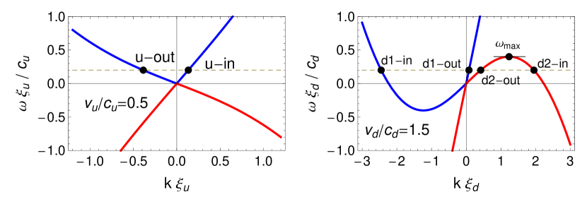
Figure 1: (Color online) Quasiparticle dispersion relation on the subsonic (left, upstream) and supersonic (right, downstream) sides. The blue (red) branches correspond to positive (negative) normalization. As in Refs. [recati2009, ; zapata2011, ; larre2012, ], $d(u)$ denotes downstream/upstream. Here, $\xi_{u(d)}$ denotes the asymptotic healing length, $c_{u(d)}$ and $v_{u(d)}$ the sound and flow velocities, and $\omega_{{\rm max}}$ the frequency above which no HR can be generated.

II Cauchy-Schwartz inequalities in Hawking Radiation

We focus on the properties of the normalized second-order correlation function, which for light is defined as loudon2000 ; walls2008

$$g_{ij}^{(2)}(\tau)\equiv\frac{\langle\hat{a}_{i}^{\dagger}(0)\hat{a}_{j}^{\dagger}(\tau)\hat{a}_{j}(\tau)\hat{a}_{i}(0)\rangle}{\langle\hat{a}_{i}^{\dagger}(0)\hat{a}_{i}(0)\rangle\langle\hat{a}_{j}^{\dagger}(0)\hat{a}_{j}(0)\rangle}\,,$$ (1)

where $\hat{a}_{i}(t)$ is the Heisenberg operator for photon mode $i$, and the average is quantum-statistical. The correlation function for classical light is obtained by removing the quantum average and replacing the Heisenberg operators $\hat{a}_{i}(t)$ by complex numbers. The following inequalities can be proven for classical light:

$$1 \leq g_{ii}^{(2)}(0),$$ (2)

$$g_{ii}^{(2)}(\tau) \leq g_{ii}^{(2)}(0),$$ (3)

$$\left[g_{ij}^{(2)}(\tau)\right]^{2} \leq g_{ii}^{(2)}(0)g_{jj}^{(2)}(0)\,,\;(i\neq j)\,.$$ (4)

These inequalities are satisfied not only classically but also by quantum thermal states at high temperature. They are also satisfied by chaotic and coherent states.

The violation of any of the above inequalities is a signature of deep quantum behavior. States violating (2) are said to show sub-Poissonian statistics. Violation of (3) reflects anti-bunching. Expression (4) is a CS inequality. States which violate it at $\tau=0$ are said to exhibit two-mode sub-Poissonian statistics. In general, the proof of (4) requires the system to be described by a positive (Glauber-Sudarshan) P function. Some quantum states such as two-mode squeezed states may not satisfy this condition and thus can violate (4). That could be the case in a collision between two BE condensates kheruntsyan2012 .

Now we turn our attention to Hawking radiation. References recati2009, ; macher2009, ; zapata2011, ; larre2012, have addressed the existence and possible detection of HR in bosonic condensates. Figure 1 shows the dispersion relation of the scattering channels following the mode notation of Refs. recati2009, ; zapata2011, ; larre2012, , to which the reader is referred for further details. A particular type of HR often considered in analog systems is the emission of $u$-out phonons as originated in the anomalous transmission from the $d2$-in channel. Hereafter, the operator $\hat{\gamma}_{i-\alpha}$ destroys a quasiparticle in the scattering state characterized by channel $i-\alpha$, with $i=u,d1,d2$ and $\alpha={\rm in,out}$. The dependence of $\hat{\gamma}_{i-\alpha}(\omega)$ on the quasiparticle frequency $\omega$ will often be understood. As is conventional in finite temperature HR setups, we assume that averages are taken for a thermal distribution of incoming quasiparticles, so that $\langle\hat{\gamma}_{i-{\rm in}}^{\dagger}(\omega)\hat{\gamma}_{j-{\rm in}}(\omega^{\prime})\rangle=n_{i}(\omega)\delta_{ij}\delta(\omega-\omega^{\prime})$, where $n_{i}(\omega)=\left[\exp(\hbar\Omega_{i}(\omega)/k_{B}T)-1\right]^{-1}$ and $\Omega_{i}(\omega)$ is the comoving frequency corresponding to the mode $i$-in at the laboratory frequency $\omega$.

We consider the equal-time second-order correlation function for the outgoing quasiparticle operators

$$\Gamma_{ij}\equiv\langle\hat{\gamma}_{i-{\rm out}}^{\text{$\dagger$}}\hat{\gamma}_{j-{\rm out}}^{\dagger}\hat{\gamma}_{j-{\rm out}}\hat{\gamma}_{i-{\rm out}}\rangle>0,$$ (5)

and define $\theta_{ij}\equiv\Gamma_{ij}/\sqrt{\Gamma_{ii}\Gamma_{jj}},\,\Theta_{ij}\equiv\Gamma_{ij}-\sqrt{\Gamma_{ii}\Gamma_{jj}}$ comm1 , noting that the CS inequality (4) is violated if and only if

$$\theta_{ij}>1\,({\rm or}\,\,\Theta_{ij}>0)\,.$$ (6)

Thus, we may use $\theta_{ij}$ ($\Theta_{ij}$) as a relative (absolute) figure of merit to quantify the degree of CS violation.

We define the complex vector $\alpha_{i}^{\dagger}\equiv(\sqrt{n_{u}}S^{*}_{iu},\sqrt{n_{d1}}S^{*}_{id1},\sqrt{n_{d2}+1}S^{*}_{id2})$, where $S_{ij}$ is the element $ij$ of the scattering matrix $S$ characterizing the transition from $j$-in to $i$-out comment1 and obeying the pseudo-unitary condition $S^{\dagger}\eta S=\eta\equiv{\rm diag}(1,1,-1)$. Specifically,

$$\left[\begin{array}[]{c}\hat{\gamma}_{u-\rm{out}}\\ \hat{\gamma}_{d1-\rm{out}}\\ \hat{\gamma}_{d2-\rm{out}}^{\dagger}\end{array}\right]=S(\omega)\left[\begin{array}[]{c}\hat{\gamma}_{u-\rm{in}}\\ \hat{\gamma}_{d1-\rm{in}}\\ \hat{\gamma}_{d2-\rm{in}}^{\dagger}\end{array}\right]\,.$$ (7)

Wick’s theorem allows us to write

$$\Gamma_{uu} = 2|\braket{\hat{\gamma}_{u-\rm{out}}^{\dagger}\hat{\gamma}_{u-\rm{out}}}|^{2}$$

$$\Gamma_{d2d2} = 2|\braket{\hat{\gamma}_{d2-\rm{out}}^{\dagger}\hat{\gamma}_{d2-\rm{out}}}|^{2}$$

$$\Gamma_{ud2} = \braket{\hat{\gamma}_{d2-\rm{out}}^{\dagger}\hat{\gamma}_{u-\rm{out}}^{\dagger}}\braket{\hat{\gamma}_{d2-\rm{out}}\hat{\gamma}_{u-\rm{out}}}$$ (8)

$$+ \braket{\hat{\gamma}_{u-\rm{out}}^{\dagger}\hat{\gamma}_{u-\rm{out}}}\braket{\hat{\gamma}_{d2-\rm{out}}^{\dagger}\hat{\gamma}_{d2-\rm{out}}}\,,$$

which leads to

$$\Gamma_{uu} = 2|\alpha_{u}|^{4}$$

$$\Gamma_{d2d2} = 2(|\alpha_{d2}|^{2}-1)^{2}$$

$$\Gamma_{ud2} = |\alpha_{u}^{\dagger}\cdot\alpha_{d2}|^{2}+|\alpha_{u}|^{2}(|\alpha_{d2}|^{2}-1)\,.$$ (9)

Making use of (5) and (9), the CS inequality (4) for outgoing quasiparticles can be rewritten as

$$|\alpha_{u}^{\dagger}\cdot\alpha_{d2}|^{2}\leq|\alpha_{u}|^{2}\left(|\alpha_{d2}|^{2}-1\right)\,,$$ (10)

which, due to the $-1$ term within the bracket, can be violated some times. Interestingly, the very possibility of violating the CS inequality (4) is a direct consequence of the anomalous character of the scattering process $d2$-in $\rightarrow$ $u$-out, because the $u(d2)$ channel has positive (negative) normalization. In fact, for the (normal) conversion $d1\leftrightarrow u$, we obtain that (4) amounts to $|\alpha_{u}^{\dagger}\cdot\alpha_{d1}|^{2}\leq|\alpha_{u}|^{2}|\alpha_{d1}|^{2}$, which is always satisfied.

The inequality (10) and pseudo-unitarity lead, after a lengthy calculation, to the equivalent relation

$$|S_{ud2}|^{2}(1+n_{u}+n_{d1}+n_{d2})\leq$$

$$|S_{d1u}|^{2}n_{d1}n_{d2}+|S_{d1d1}|^{2}n_{u}n_{d2}+|S_{d1d2}|^{2}n_{u}n_{d1}$$

$$+|S_{d2d1}|^{2}n_{u}+|S_{d2u}|^{2}n_{d1}\,.$$ (11)

A similar inequality can be derived for the other anomalous process, $d1\leftrightarrow d2$ (Andreev reflection zapata2009 ), by interchanging $u$ and $d1$ in (11).

In the conventional ($\omega$ = 0) peak of the Hawking spectrum $|S_{ud2}(\omega)|^{2}$, the scattering matrix elements diverge as $|S_{ij}(\omega)|\sim 1/\sqrt{\omega}$ with $i$ arbitrary and $j=d1,d2$ . By contrast, $S_{iu}(\omega)$ in the same limit ($\omega\rightarrow 0^{+}$) saturates to a nonzero constant (the asymptotic behavior of the $S-$matrix coefficients is discussed in Appendix A). On the other hand, the only occupation factor which diverges is $n_{u}(\omega)\sim 1/\omega$, because $\Omega_{u}(\omega)$ is the only comoving frequency that vanishes for small $\omega$. From pseudo-unitarity it follows that $|S_{ud2}|^{2}-|S_{d2d1}|^{2}=|S_{d2u}|^{2}-|S_{d1d2}|^{2}$. We conclude that (11) cannot be violated in the $\omega\rightarrow 0^{+}$ region. This argument relies solely on the presence of a uniform condensate flow connecting the subsonic and supersonic asymptotic regions, and not on other details of the scattering structure.

It can also be proven that there is no violation in the $\omega\rightarrow\omega^{-}_{\rm max}$ region, where $\theta_{ud2}=1/2+O\left(\sqrt{\omega_{\rm max}-\omega}\right)$. This leaves us with only the central frequency region in the quest for CS violation. We know of no structure other than resonant BH zapata2011 , which is able to display peaks in that central region; see Sec. III for more details.

The inequality (11) is manifestly violated at temperature $T=0$ and $\omega\neq 0$ provided $S_{ud2}\neq 0$, which further reflects the direct link between CS violation and HR. In this limit, the condition (6) is equivalent to

$$\theta_{ud2}=\frac{|S_{d2d2}|^{2}-1/2}{|S_{d2d2}|^{2}-1}>1\,,\,\,\Theta_{ud2}=|S_{ud2}|^{2}>0\,,$$ (12)

where pseudo-unitarity has again been invoked. The condition (12) is guaranteed to be satisfied whenever $S_{ud2}\neq 0$ (in that case, pseudo-unitarity requires $|S_{d2d2}|>1$). Finally, we note that $\theta_{d1d2}=\theta_{ud2}$ and $\Theta_{d1d2}=|S_{d1d2}|^{2}$ at zero temperature.

A device producing HR works like a nondegenerate parametric amplifier, which is known to generate squeezing from vacuum. However, sources other than vacuum may also generate squeezing and ultimately CS violation walls2008 . In particular, the absolute amount of CS violation for a given frequency often increases initially as the temperature is raised from zero, eventually reaching a maximum and decreasing to zero at high temperatures, as can be guessed from Eq. (11). Therefore, one may wonder whether the CS violation here contemplated would provide conclusive evidence of spontaneous (zero-point) HR radiation. The answer is yes, as we argue below.

Wick’s theorem can again be invoked to write $\Gamma_{ij}$ in terms of first-order correlation functions such as $\langle\hat{\gamma}_{i-{\rm out}}^{\dagger}\hat{\gamma}_{j-{\rm out}}\rangle$ or $\langle\hat{\gamma}_{i-{\rm out}}\hat{\gamma}_{j-{\rm out}}\rangle$ [see Eq. (8)], here generically referred to as $\rho_{ij}$ comm2 . The thermal contribution is $\rho_{ij}^{{\rm th}}\equiv\rho_{ij}-\rho_{ij}^{0}$, with $\rho_{ij}^{0}$ the zero-temperature value (average over incoming vacuum). If one neglects the zero-point contributions by approximating $\rho_{ij}\simeq\rho_{ij}^{{\rm th}}$, then one arrives at a modified version of (11) where only the terms quadratic in the $n_{i}$’s survive. The resulting inequality is always satisfied. We conclude that CS violation requires vacuum fluctuations.

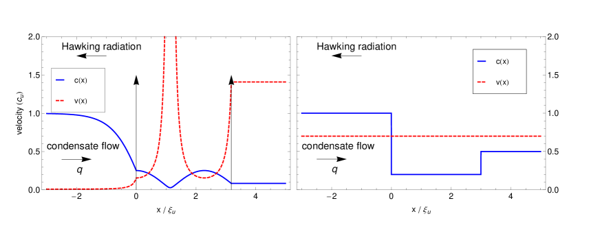
Figure 2: (Color online) Scheme of the double-barrier configuration (left) and the configuration with two discontinuities in the otherwise flat density configuration (right).

The upshot of this discussion is that the detection of a CS inequality violation can be regarded as a smoking gun for the presence of spontaneous HR. In other words, the spontaneous signal is the cause of the quantum behavior as reflected in the violation of the classical inequalities. This contrasts with other schemes in which the spontaneous signal cannot be distinguished unambiguously from the stimulated (or thermal) signal, which has, in this sense, a classical behavior and thus would never originate the CS violation by itself.

We may define the violation temperature $T_{v}$ as the highest temperature at which (11) is violated [(6) is satisfied] and try to identify some trends in its behavior. We note that, for a double-barrier structure zapata2011 , if the upstream current is small (kinetic contribution to total chemical potential on subsonic side is small), then for $\omega\gtrsim\omega_{{\rm max}}/2$ the comoving frequencies of the various channels are comparable to the comoving chemical potential on the subsonic side, $\mu$.

If the conversion from negative to positive normalization is weak, then $|S_{d2d2}|$ is close to unity and from pseudo-unitarity it can be proven that all the $S$-matrix elements appearing in (11) are small except for the relation $|S_{d1u}|^{2}+|S_{d1d1}|^{2}\simeq 1$. If $\ell\equiv-\log|S_{ud2}|\gg 1$ we obtain a low violation temperature, $k_{B}T_{v}\sim\mu/\ell\ll\mu$.

Conversely, also within the case of a double-barrier structure and for low currents, we find numerically that for the highest nonzero-frequency HR peaks (where $|S_{ud2}|\!\!\gg\!\!1$) the approximate relation $|S_{ud2}|\simeq|S_{d2u}|\gg|S_{d2d1}|$ applies in the vast majority of cases. At the same time, $|S_{ud2}|\gg|S_{d1j}|$ for all $j$, which implies that the violation temperature satisfies $k_{B}T_{v}\sim\mu|S_{ud2}|^{2}/S_{d1}^{2}\gg\mu$, where $S_{d1}\equiv\max_{j}\{|S_{d1j}|\}$. Thus, $T_{v}(\omega)$ is expected to be large near the peak frequency $\omega_{0}$. Non-resonant structures can also show CS violation at nonzero temperatures. However, even if the relative violation (as measured by $\theta_{ud2}$) is significant, the absolute amount of violation (as measured by $\Theta_{ud2}$) turns out to be negligible, as discussed later.

Another important advantage of resonant peaks is that, at their relatively high frequency, the phononic signal is approximately proportional to the atomic signal, the latter being directly measurable in a time-of-flight (TOF) experiment. In Appendix B technical details are given for the definition of atomic signals and their relation to phonon measurements. Assuming that the subsonic and supersonic TOF signals can be experimentally detached, near the peak at $\omega=\omega_{0}$, and neglecting finite-size effects, the atom operators can be approximated as:

$$\hat{c}_{u}(p_{u}\equiv q_{u}+k_{u-{\rm out}}) \sim \hat{\gamma}_{u-{\rm out}}(\omega)$$ (13)

$$\hat{c}_{d}(p_{d1}\equiv q_{d}+k_{d1-{\rm out}}) \sim \hat{\gamma}_{d1-{\rm out}}(\omega)$$ (14)

$$\hat{c}_{d}(p_{d2}\equiv q_{d}-k_{d2-{\rm out}}) \sim \hat{\gamma}_{d2-{\rm out}}(\omega)\,,$$ (15)

where $\hat{c}_{u/d}(k)$ annihilates an atom of momentum $k$ on side $u/d$. Here, $k_{i-{\rm out}}$ is the comoving quasiparticle momentum at the laboratory frequency $\omega$ in the $i-{\rm out}$ channel, and $q_{u/d}$ is the condensate momentum per atom on each side. The proportionality factors not shown in (13)-(15) cancel in the CS violation condition (6) for $\theta_{ud2}$ and $\theta_{d1d2}$.

For example, the approximations (13),(15) apply whenever $|S_{ud2}(\omega_{0})|^{2}\!\gg\!1$, because the Hawking signal has to stand out above that of the depletion cloud zapata2011 . For completeness, we note that (14) and (15) apply if $|S_{d1d2}(\omega_{0})|^{2}\!\gg\!1$.

From (12) and the pseudo-unitarity relation $|S_{ud2}|^{2}+|S_{d1d2}|^{2}+1=|S_{d2d2}|^{2}$, it may appear that a shortcoming of a large peak is its small relative degree of CS violation, as reflected in $\theta_{ud2}$ lying slightly above unity, which can be generally inferred from the bound

$$\theta_{ud2}-1\leq\frac{1}{2(|\alpha_{d2}|^{2}-1)}\,.$$ (16)

However, this does not imply that the experimental signal is necessarily small. Quite the opposite, the absolute amount of violation (as measured by $\Theta_{ud2}$) can be quite large, as (12) directly reveals. A similar analysis can be performed for the other anomalous process, $d1\leftrightarrow d2$.

We can define, in analogy to (5), the atomic correlation function

$$G_{ud2}(\omega)\equiv\langle\hat{c}_{u}^{\dagger}(p_{u})\hat{c}_{d}^{\dagger}(p_{d2})\hat{c}_{d}(p_{d2})\hat{c}_{u}(p_{u})\rangle\,,$$ (17)

and similarly for the other $G_{ij}$, where $i,j=u,d1,d2$, and $p_{i}(\omega)$ is defined in (13)-(15). It can be shown (see Appendix B) that a sufficient condition for (6) is

$$z_{ij}>1\,,\,\,Z_{ij}>0\,,$$ (18)

where $z_{ij}\equiv G_{ij}/\sqrt{G_{ii}G_{jj}}$ and $Z_{ij}\equiv G_{ij}-\sqrt{G_{ii}G_{jj}}$.

III CS violation by Hawking Radiation in resonant structures

In order to study CS violation by HR in resonant structures, we focus on two models. In the first case, a double delta-barrier potential $V(x)=Z[\delta(x)+\delta(x-d)]$ is introduced separating the subsonic from the supersonic regions, where $d$ is the distance between the barriers and $Z$ measures their strength. This structure was already explored in Ref. zapata2011, and is schematically depicted in the left panel of Fig. 2. Given these parameters, only a discrete number of currents are compatible with the existence of two asymptotic regions of uniform density and flow speed, one subsonic and one supersonic. Even though the speed of sound is only properly defined for sufficiently flat regions, by extending its definition in terms of the local density of the condensate to generally nonuniform profiles, $c(x)=[gn(x)/m]^{1/2}$, this speed of sound will cross the flow velocity at least once. Here, $g$ is the one-dimensional coupling constant, $n(x)$ is the linear atom density, and $m$ the atom mass. As expected from the study in Ref. zapata2011, , the HR spectrum displays resonant peaks, its number increasing roughly with the barrier separation. We will argue that these peaks are good candidates to exhibit CS violations.

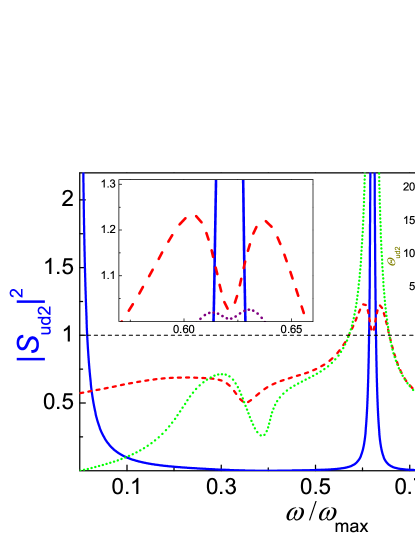
Figure 3: (Color online) Hawking radiation for a condensate leaking through a double barrier structure like that studied in Ref. zapata2011, and shown in the left Fig. [2]. The strength of both delta barriers is $Z=2.2\hbar^{2}/m\xi_{u}$. They are separated by a distance $d=3.62\xi_{u}$. The flow is such that $q_{u}\xi_{u}=0.01$ and $\omega_{{\rm max}}=0.99\mu/\hbar$. Solid blue: zero-temperature HR spectrum $|S_{ud2}(\omega)|^{2}$. Dashed red: $\theta_{ud2}(\omega)$ at temperature $T=\mu/k_{B}$, where $\mu$ is the comoving chemical potential on the subsonic side. Dotted green: maximum violation temperature $T_{v}(\omega)$ in units of $\mu/k_{B}$. Not shown in the figure, $T_{v}(\omega)$ rises up to $T_{v}(\omega_{0})\simeq 21\mu/k_{B}$, where $|S_{ud2}(\omega_{0})|^{2}\simeq 8$. Left inset: Zoom of the peak region, with $T_{v}(\omega)$ removed and $z_{ud2}(\omega)$ (relative atom CS violation) added (dotted purple). Right inset: Same as left inset; it shows $\Theta_{ud2}(\omega)$ (dashed-dotted brown) and $Z_{ud2}(\omega)$ (dashed purple), which measure the absolute amount of CS violation in the phonon and atom signals.

The other model considered in this work is a resonant generalization of a flat profile configuration, first considered in Ref. recati2009, and schematically depicted in the right panel of Fig. 2. In that scenario, the GP wave function is everywhere the same plane wave, $\Psi_{0}(x)=\sqrt{n_{0}}e^{iqx}$, with flow speed $v=\hbar q/m$. Therefore, the condensate density, velocity and current are all constant along the BH structure. Both the one-dimensional coupling strength $g\left(x\right)$ and the external potential $V\left(x\right)$ are space dependent and chosen in such a way that $g^{\prime}(x)n_{0}+V^{\prime}(x)=0$. We consider a spatial dependence with three regions within each of which the sound speed, $c(x)=[g(x)n_{0}/m]^{1/2}$, is constant. Specifically, we take $c(x<0)=c_{1}$, $c(0\leq x\leq L)=c_{2}$, $c(x>L)=c_{3}$, with $c_{1}>v>c_{3}$. That is, the left-most (right-most) region is subsonic (supersonic). The middle region, with speed of sound $c_{2}$, can be subsonic of supersonic depending on the externally chosen parameters. This highly idealized model yields closed formulas for many quantities of interest.

In Fig. 3 we plot, for a double delta-barrier structure, the zero temperature HR spectrum $|S_{ud2}(\omega)|^{2}$, together with $\theta_{ud2}(\omega)$ (at $k_{B}T=\mu$) and the violation temperature $T_{v}(\omega)$. The left inset magnifies the peak region and includes $z_{ud2}(\omega)$, which measures the relative amount of CS violation in the atomic signal. The right inset shows $\Theta_{ud2}(\omega)$ and $Z_{ud2}(\omega)$, i.e., the absolute amount of CS violation by the phonon and atom signals. These graphs indicate that the considered structure is a promising scenario for the unambiguous detection of spontaneous HR.

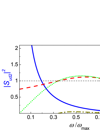
Figure 4: (Color online) Same as Fig. 3 for a setup with a single delta barrier of strength $Z=0.62\hbar^{2}/m\xi_{u}$ and a uniform interaction, with flow $q_{u}\xi_{u}=0.3$ and $\omega_{{\rm max}}=0.6\mu/\hbar$. Atomic CS violation is not found for this setup.

Figure 4 shows the corresponding curves for a single delta-barrier BH configuration. The HR spectrum is unstructured, with a single peak at $\omega=0$. The CS inequality can be violated at the relatively high temperature $T=\mu/k_{B}$ within a considerable frequency range. However, the smallness of the absolute phonon violation signal suggests that nonresonant structures are not good candidates for the observation of CS violation. In the cases we have explored, we have not found atomic CS violation at the temperature $T=\mu/k_{B}$.

Figure 5 shows the same curves as those of Fig. 3 but for a setup with a flat density profile such as that depicted in the right Fig. 2. The absolute CS violation is here considerably smaller than in Fig. 3 but could still be observable.

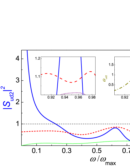
Figure 5: (Color online) Same as Fig. 3 but for $T=0.6\mu/k_{B}$ and for a structure without barriers but with two sharp variations in the local speed of sound, which takes the successive values $c_{u},0.43c_{u},0.6c_{u}$, as depicted in the right Fig. 2. The intermediate region has a length $L=26\xi_{u}$. The flow is such that $q_{u}\xi_{u}=0.95$ and $\omega_{{\rm max}}=0.18\mu/\hbar$. This is a resonant generalization of the model first studied in Ref. balbinot2008, , where only one sound-speed discontinuity was considered.

IV Conclusions

In conclusion, we find that violation of the Cauchy-Schwartz inequalities in the HR of strongly peaked spectrum (such as that emitted by a double-barrier sonic BH) may provide a convenient route to the unambiguous observation of the zero-point contribution. In some setups, the violation of CS inequalities is large enough to be detectable by the direct observation of second-order correlation functions in an atom time-of-flight experiment. The large absolute CS violation is absent in nonresonant structures such as that formed by a single-barrier sonic BH. In particular, the relevant CS violation cannot occur near the conventional, zero-frequency HR peak universally shown by all one-dimensional black-hole structures.

We thank D. Guery-Odelin, R. Parentani and C. Westbrook for valuable discussions. Support from MINECO (Spain) through grant FIS2010-21372 and from Comunidad de Madrid through grant MICROSERES-CM (S2009/TIC-1476) is also acknowledged.

Appendix A Limiting behavior of scattering matrix elements near thresholds

In this Appendix we study the asymptotic behavior of the amplitudes of the scattering matrix coefficients, $|S_{ij}\left(\omega\right)|$, close to the thresholds of the HR spectrum, i.e., in the limits $\omega\rightarrow 0^{+}$ and $\omega\rightarrow\omega^{-}_{\rm max}$. In the following, we adopt units $\hbar=m=1$. In the asymptotic regions where the condensate flow is uniform, the condensate wave function is of the form $\Psi_{0}(x)=\sqrt{n_{r}}e^{i(q_{r}x+\alpha_{r})}$, where $r=u,d$ labels the asymptotic region at $x\rightarrow\text{$\pm\infty$}$. The asymptotic plane-wave solutions to the Bogoliubov-de Gennes (BdG) equations at a given frequency $\omega$ (scattering channels) can be written as

$$s_{a,\omega}\left(x\right) := \frac{e^{ik_{a}\left(\omega\right)x}}{\sqrt{2\pi|w_{a}\left(\omega\right)|}}\left[\begin{array}[]{c}e^{iq_{r}x}u_{a}(\omega)\\ e^{-iq_{r}x}v_{a}(\omega)\end{array}\right]$$ (21)

$$u_{a}(\omega) = C_{a}\left\{\frac{k_{a}^{2}\left(\omega\right)}{2}+[\omega-q_{r}k_{a}\left(\omega\right)]\right\}$$

$$v_{a}(\omega) = C^{*}_{a}\left\{\frac{k_{a}^{2}\left(\omega\right)}{2}-[\omega-q_{r}k_{a}\left(\omega\right)]\right\}\,$$

$$C_{a} = \frac{e^{i\alpha_{r}}}{\sqrt{2k_{a}^{2}\left(\omega\right)\left|\omega-q_{r}k_{a}\left(\omega\right)\right|}}.$$ (22)

We also refer to $s_{a,\omega}\left(x\right)$ as the spinor (two-component wave function) of the propagating mode or scattering channel $a$ at frequency $\omega$.

Here, the mode index $a$ labels the four wave vectors which are solutions of the Bogoliubov’s dispersion relation

$$\left[\omega-q_{r}k_{a}\left(\omega\right)\right]^{2}=c_{r}^{2}k_{a}^{2}\left(\omega\right)+k_{a}^{4}\left(\omega\right)/4$$ (23)

for a given frequency $\omega>0$ in the region of index $r=u,d$, while $w_{a}\left(\omega\right):=\left[dk_{a}\left(\omega\right)/d\omega\right]^{-1}$ is the group velocity of mode $a$ which lives in the asymptotic region $r$. The sound velocities are $c_{r}=\sqrt{g_{r}n_{r}}$, where $g_{r}$ is the corresponding asymptotic value of the coupling constant $g(x)$. In the case of propagating modes, the index $a$ is of the form $a=i-\alpha$ (with $i=u,d1,d2$ and $\alpha={\rm in,out}$) and the normalization is $\intop\mathrm{d}x\,s_{a,\omega}^{\dagger}\left(x\right)\sigma_{z}s_{a,\omega^{\prime}}\left(x\right)=\pm\delta\left(\omega-\omega^{\prime}\right)$, with $\sigma_{z}$ the Pauli matrix. The symbol $\pm$ stands for positive or negative normalization. In the subsonic region, there are only two propagating modes (labeled $u-{\rm in}$ and $u-{\rm out}$), both with positive normalization, the other two solutions of (23) describing an evanescent wave and an (unphysical) exploding one. In the supersonic region, where four propagating modes exist, the two pairs of modes with positive (negative) normalization are denoted as $d1(d2)$, each pair consisting of an “in” and an “out” channel.

In the nonhomogeneous case, the field operator in the BdG approximation can be written as $\hat{\Psi}(x)=\Psi_{0}(x)+\delta\hat{\Psi}(x)$ with zapata2011 :

$$\delta\hat{\Psi}(x) = \int_{0}^{\infty}d\omega\sum_{a={\rm u-\rm{in},d1-\rm{in}}}[u_{a,\omega}(x)\hat{\gamma}_{a}(\omega)$$ (24)

$$+ v_{a,\omega}^{*}(x)\hat{\gamma}_{a}^{{\dagger}}(\omega)]+\int_{0}^{\omega_{{\rm max}}}d\omega[u_{{\rm{d2-\rm{in},\omega}}}(x)\hat{\gamma}_{{\rm{d2-\rm{in}}}}^{{\dagger}}(\omega)$$

$$+ v_{{\rm{d2-\rm{in},\omega}}}^{*}(x)\hat{\gamma}_{{\rm{d2-\rm{in}}}}(\omega)]\,.$$

A similar expression can be written in terms of the “out” states. Here, the spinors $z_{a,\omega}(x):=\left[u_{a,\omega}(x),v_{a,\omega}(x)\right]^{\intercal}$ are solutions to the BdG equations at a given frequency $\omega$, carrying unit flux in the incoming channels $a=d1,d2,u-{\rm in}$ which characterize them. As expected from scattering states, they contain $S$-matrix coefficients describing the transition from the incoming to the outgoing modes. For instance,

$$z_{d2-\rm{in},\omega}\left(x\rightarrow-\infty\right) = S_{ud2}\left(\omega\right)s_{u-\rm{out},\omega}\left(x\right)$$ (25)

$$z_{d2-\rm{in},\omega}\left(x\rightarrow\infty\right) = s_{d2-\rm{in},\omega}\left(x\right)$$

$$+ S_{d1d2}\left(\omega\right)s_{d1-\rm{out},\omega}\left(x\right)$$

$$+ S_{d2d2}\left(\omega\right)s_{d2-\rm{out},\omega}\left(x\right)\,.$$

Similar expressions can be written for the other retarded scattering states.

When $\omega\rightarrow 0^{+}$, both the “$u-$in” and the three “out” scattering channels have the property $k_{a}\propto\omega$ (see Fig. 1), where $k_{a}$ is the momentum of the scattering channel $a$. From (22) we infer that the spinors of these four scattering channels behave as $\propto z_{0}\left(x\right)/\sqrt{\omega}$ with corrections $\sim\sqrt{\omega}$, where

$$z_{0}(x)\equiv\left[\Psi_{0}(x),-\Psi_{0}^{*}(x)\right]^{\intercal}\,,$$ (26)

is but the zero-mode spinor which solves the BdG equations for $\omega=0$. The other spinors do not show this behavior for vanishing $\omega$. Using Cramer’s rule to match the left and right solutions, one finds that $\left|S_{ij}\left(\omega\right)\right|\propto 1/\sqrt{\omega}$ for $i,j=d1,d2$. To obtain the behavior of the other scattering matrix coefficients, it is crucial to note the zero-mode character of $z_{0}\left(x\right)$. One must also use the property that, in the scattering region (that between the asymptotic subsonic and supersonic regions), at least one linear combination of the four solutions tends to the zero-mode when $\omega\rightarrow 0^{+}$, within corrections to the spinor $z_{0}(x)$ of order $\omega$. This is guaranteed because in the BdG equations $\omega$ enters as a nonsingular parameter, i.e., a parameter that is not multiplying the highest order derivative of the differential equation. Here we have used a theorem (sometimes referred to as Poincaré’s theorem) on the analytic dependence of a solution to a differential equation on its parameters (see Refs. arnold1992, ; kaltchev2011, ).

Using these results, the same type of reasoning as before leads to $\left|S_{ui}\left(\omega\right)\right|\propto 1/\sqrt{\omega}$ for $i=d1,d2$ and to a nondivergent amplitude for the remaining matrix elements ($S_{iu}$ with $i=d1,d2$).

In the opposite threshold, $\omega\rightarrow\omega^{-}_{\rm max}$, the only spinors that show irregular behavior are those involving the $d2$ mode. They become proportional to each other because $k_{d2-\rm{in/out}}\left(\omega\right)=k_{d2}(\omega_{\rm max})\pm O(\sqrt{\omega_{\rm max}-\omega})$ and hence, the group velocity vanishes as $\sim\sqrt{\omega_{\rm max}-\omega}$. The corresponding spinors behave as $s_{d1-{\rm in/out},\omega}(x)\propto s_{\omega_{\rm max}}\left(x\right)\left(\omega_{\rm max}-\omega\right)^{-1/4}+O\left(\omega_{\rm max}-\omega\right)^{1/4}$ where $s_{\omega_{\rm max}}\left(x\right)$ is the value of the spinor evaluated at $\omega_{\rm max}$. Using again Cramer’s rule, it can be shown that $S_{ud2}\left(\omega\right),S_{d1d2}\left(\omega\right),S_{d2u}\left(\omega\right),S_{d2d1}\left(\omega\right)\propto\left(\omega_{\rm max}-\omega\right)^{1/4}$, while $S_{d2d2}\left(\omega\right)=-1+O(\sqrt{\omega_{\rm max}-\omega})$ .

Appendix B Correlation between phonon and atomic time-of-flight signals.

For a given frequency $\omega>0$, we may define $p_{u}(\omega)\equiv q_{u}+k_{u-{\rm out}}(\omega)$, $p_{d2}(\omega)\equiv q_{d}-k_{d2-{\rm out}}(\omega)$ [see Eqs. (13),(15) and Appendix A for the mode notation] as the corresponding atomic wave vectors. In a time-of-flight (TOF) experiment, we require the atomic wave vectors from the upstream (downstream) region to be negative (positive), i.e., we just consider frequencies where $p_{u}(\omega)<0$ comm3 . In particular, this must be valid at the peak frequency $\omega=\omega_{0}$, i.e., one must have $p_{u}(\omega_{0})<0$. If all these conditions are fulfilled, then there is no contribution from the condensate wave function to the atomic signals.

We define the atom destruction operators as

$$\hat{c}_{u}\left(p\right) \equiv\int\mathrm{d}x\,f_{u}^{*}\left(x\right)e^{-ipx}\delta\hat{\Psi}(x)$$

$$\hat{c}_{d}\left(p\right) \equiv\int\mathrm{d}x\,f_{d}^{*}\left(x\right)e^{-ipx}\delta\hat{\Psi}(x),$$ (27)

where $f_{r}\left(x\right)$ are normalized functions ($\int\mathrm{d}x|f_{r}(x)|^{2}=1$) localized only in the asymptotic $r=u,d$ regions and their Fourier transforms are $f_{r}(k)=\frac{1}{\sqrt{2\pi}}\int\mathrm{d}x~{}e^{-ikx}f_{r}\left(x\right)$. For simplicity, we assume that they are of the form

$$f_{r}(x)=\frac{1}{\sqrt{L_{r}}}f\left(\frac{x-x_{r}}{L_{r}}\right)\,,$$ (28)

where $f$ is a symmetric and real dimensionless function, $x_{r}$ is the point at which the asymptotic region $r$ is assumed to be centered, and $L_{r}$ is the typical size of that region. We assume that both such lengths are much greater than the corresponding healing lengths ($L_{r}\gg\xi_{r}$), so that $f_{r}(k)$ are well peaked at zero momentum. Also, we suppose that the scattering region is much smaller than the asymptotic regions. Then, the atomic operators can be approximated as

$$\hat{c}_{u}\left(p_{u}\left(\omega\right)\right) \simeq \int\mathrm{d}\omega^{\prime}~{}f^{*}_{u}(k_{u-\rm{out}}(\omega^{\prime})-k_{u-\rm{out}}(\omega))\frac{u_{u-\rm{out}}(\omega^{\prime})}{\left|w_{u-\rm{out}}\left(\omega^{\prime}\right)\right|^{1/2}}\hat{\gamma}_{u-\rm{out}}(\omega^{\prime})$$

$$+ f^{*}_{u}(-k_{u-\rm{in}}(\omega^{\prime})-k_{u-\rm{out}}(\omega))\frac{v_{u-\rm{in}}^{*}(\omega^{\prime})}{|w_{u-\rm{in}}\left(\omega^{\prime}\right)|^{1/2}}\hat{\gamma}_{u-\rm{in}}^{{\dagger}}(\omega^{\prime})$$

$$\hat{c}_{d}\left(p_{d2}\left(\omega\right)\right) \simeq \int_{0}^{\omega_{\rm max}}\mathrm{d}\omega^{\prime}~{}f^{*}_{d}(k_{d2-\rm{out}}(\omega)-k_{d2-\rm{out}}(\omega^{\prime}))\frac{v_{d2-\rm{out}}^{*}(\omega^{\prime})}{|w_{d2-\rm{out}}\left(\omega^{\prime}\right)|^{1/2}}\hat{\gamma}_{d2-\rm{out}}(\omega^{\prime})$$ (29)

$$+ \int~{}\mathrm{d}\omega^{\prime}~{}f^{*}_{d}(k_{d2-\rm{out}}(\omega)-k_{d1-\rm{out}}(\omega^{\prime}))\frac{v_{d1-\rm{out}}^{*}(\omega^{\prime})}{|w_{d1-\rm{out}}\left(\omega^{\prime}\right)|^{1/2}}\hat{\gamma}_{d1-\rm{out}}^{{\dagger}}(\omega^{\prime}),$$

From these two expressions, it can be shown that, if $|S_{ud2}(\omega_{0})|^{2}\!\gg\!1$, then the main contribution to the atomic operators near the peak frequency ($\omega=\omega_{0}$) comes from their respective phononic counterparts, i.e., $\hat{c}_{u}\left(p_{u}\left(\omega_{0}\right)\right)\sim\hat{\gamma}_{u-\rm{out}}(\omega_{0})$ and $\hat{c}_{d}\left(p_{d2}\left(\omega_{0}\right)\right)\sim\hat{\gamma}_{d2-\rm{out}}(\omega_{0})$, as expressed in the main text [see Eqs. (13) and (15)]. These approximate operator relations are physically appealing but are not used in our calculations.

From Eq. (29) and its preceding discussion, we can calculate the expectation values that are necessary to compute the second-order correlation functions, namely,

$$\braket{\hat{c}_{u}^{\dagger}\left(p_{u}\left(\omega\right)\right)\hat{c}_{u}\left(p_{u}\left(\omega\right)\right)} = |u_{u-\rm{out}}(\omega)|^{2}|\alpha_{u}(\omega)|^{2}$$

$$+ |v_{u-\rm{in}}(\omega_{uu}(\omega))|^{2}[1+n_{u}(\omega_{uu}(\omega))]$$

$$\braket{\hat{c}_{d}^{\dagger}\left(p_{d2}\left(\omega\right)\right)\hat{c}_{d}\left(p_{d2}\left(\omega\right)\right)} = |v_{d2-\rm{out}}(\omega)|^{2}[|\alpha_{d2}(\omega)|^{2}-1]$$

$$+ |v_{d1-\rm{out}}(\omega_{d1d2}(\omega))|^{2}[|\alpha_{d1}(\omega_{d1d2}(\omega))|^{2}+1]$$

$$\braket{\hat{c}_{d}\left(p_{d2}\left(\omega\right)\right)\hat{c}_{u}\left(p_{u}\left(\omega\right)\right)} = [\alpha_{d2}^{{\dagger}}(\omega)\cdot\alpha_{u}(\omega)]u_{u-\rm{out}}(\omega)v_{d2-\rm{out}}^{*}(\omega)F(\omega),$$ (30)

where $\omega_{d1d2}(\omega)=\omega_{d1}(k_{d2-\rm{out}}(\omega))$ and $\omega_{uu}(\omega)=\omega_{u}(-k_{u-\rm{out}}(\omega))$, with $\omega_{i}(k)$ the dispersion relation of scattering channel $i$ (see Fig. 6) . The overlap function is

$$F(\omega) = \int\mathrm{d}k~{}f_{u}^{*}\left(\frac{k}{\rho(\omega)}\right)f_{d}^{*}\left(k\rho(\omega)\right)$$

$$= \frac{1}{\sqrt{L_{u}L_{d}}}\int\mathrm{d}x\,f\left(\frac{\rho\left(\omega\right)x+x_{u}}{L_{u}}\right)f\left(\frac{\rho\left(\omega\right)^{-1}x-x_{d}}{L_{d}}\right)\,,$$

$$\rho(\omega) \equiv \left|\frac{w_{u-\rm{out}}(\omega)}{w_{d2-\rm{out}}(\omega)}\right|^{1/2}\,.$$ (31)

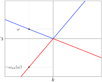
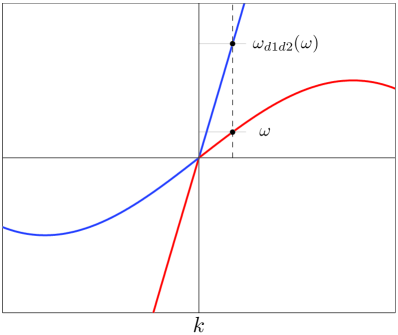
Figure 6: (Color online) Scheme that shows graphically the values of $\omega_{d1d2}(\omega)$ and $-\omega_{uu}(\omega)$. See Fig. 1 for mode notation.

As we are assuming that the size of the asymptotic regions are much larger than the size of the scattering region, we can take $x_{d}/L_{d}=-x_{u}/L_{u}\simeq 1/2$. The integral $F\left(\omega\right)$ can be interpreted as the scalar product of two normalized functions, so $F(\omega)\leq 1$. This inequality saturates for $\omega$ such that $\rho(\omega)=\sqrt{L_{u}/L_{d}}$. In particular, we can choose the size of both asymptotic regions to be such that the saturation is achieved at the peak frequency, i.e., such that $\rho(\omega_{0})=\sqrt{L_{u}/L_{d}}$ and therefore $F(\omega_{0})=1$. The criterion $\rho(\omega)=\sqrt{L_{u}/L_{d}}$ has a straightforward physical interpretation. The phonon operators are evaluated in the frequency domain. The frequency resolution near a given frequency for both wave packets is given by $\Delta\omega_{u-\rm{out}/d2-\rm{out}}=|w_{u-\rm{out}/d2-\rm{out}}\left(\omega\right)|\Delta k_{u/d}$. The resolution in momentum space is $\Delta k_{r}\sim 1/L_{r}$. We are correlating the phonon operators of $u-\rm{out}$ and $d2-\rm{out}$ modes in the vicinity of a given frequency, so the maximum correlation is achieved when $\Delta\omega_{u-\rm{out}}=\Delta\omega_{d2-\rm{out}}$ and this implies the criterion mentioned above.

Then, using Wick’s theorem, the correlation functions can be written in terms of these expectation values as:

$$G_{uu}(\omega) = \braket{\hat{c}_{u}^{\dagger}\left(p_{u}\right)\hat{c}^{\dagger}_{u}\left(p_{u}\right)\hat{c}_{u}\left(p_{u}\right)\hat{c}_{u}\left(p_{u}\right)}$$

$$= 2|\braket{\hat{c}_{u}^{\dagger}\left(p_{u}\right)\hat{c}_{u}\left(p_{u}\right)}|^{2}$$

$$G_{d2d2}(\omega) = \braket{\hat{c}_{d}^{\dagger}\left(p_{d2}\right)\hat{c}_{d}^{\dagger}\left(p_{d2}\right)\hat{c}_{d}\left(p_{d2}\right)\hat{c}_{d}\left(p_{d2}\right)}$$ (32)

$$= 2|\braket{\hat{c}_{d}^{\dagger}\left(p_{d2}\right)\hat{c}_{d}\left(p_{d2}\right)}|^{2}$$

$$G_{ud2}(\omega) = \braket{\hat{c}_{d}^{\dagger}\left(p_{d2}\right)\hat{c}_{u}^{\dagger}\left(p_{u}\right)\hat{c}_{d}\left(p_{d2}\right)\hat{c}_{u}\left(p_{u}\right)}$$

$$= \braket{\hat{c}_{d}^{\dagger}\left(p_{d2}\right)\hat{c}_{u}^{\dagger}\left(p_{u}\right)}\braket{\hat{c}_{d}\left(p_{d2}\right)\hat{c}_{u}\left(p_{u}\right)}$$

$$+ \braket{\hat{c}_{d}^{\dagger}\left(p_{d2}\right)\hat{c}_{d}\left(p_{d2}\right)}\braket{\hat{c}_{u}^{\dagger}\left(p_{u}\right)\hat{c}_{u}\left(p_{u}\right)}\,.$$

In this language, the violation of the atom CS inequality reads $G_{ud2}>\sqrt{G_{uu}G_{d2d2}}$. Now, comparing (30) and (B) with (8) and (9), one can infer that:

$$\frac{G_{ud2}}{\sqrt{G_{uu}G_{d2d2}}}<\frac{\Gamma_{ud2}}{\sqrt{\Gamma_{uu}\Gamma_{d2d2}}}$$ (33)

i.e.

$$z_{ud2}<\theta_{ud2}\,.$$ (34)

A similar proof can be invoked for the other index pairs $i\neq j$, the case $i=j$ being trivial. We conclude that the violation of the atom CS inequality is a sufficient condition for the same violation in the phonon signal.

References

- (1) S. W. Hawking, Nature 248, 30 (1974); Commun. Math. Phys. 43, 199 (1975).
- (2) W. G. Unruh, Phys. Rev. D 14, 870 (1976).
- (3) W. G. Unruh, Phys. Rev. Lett. 46, 1351 (1981).
- (4) U. Leonhardt, T. Kiss, and P. Öhberg, J. Opt. B 5, S42 (2003).
- (5) U. Leonhardt, T. Kiss, and P. Öhberg, Phys. Rev. A 67, 033602 (2003).
- (6) R. Balbinot, A. Fabbri, S. Fagnocchi, A. Recati and I. Carusotto, Phys. Rev. A 78, 021603 (2008).
- (7) I. Carusotto, S. Fagnocchi, A. Recati, R. Balbinot and A. Fabri, New J. Phys. 10, 103001 (2008).
- (8) J. Macher and R. Parentani, Phys. Rev. A 80, 043601 (2009).
- (9) S. Finazzi and R. Parentani, New J. Phys. 12, 095015 (2010).
- (10) A. Coutant and R. Parentani, Phys. Rev. D 81, 084042 (2010).
- (11) O. Lahav, A. Itah, A. Blumkin, C. Gordon, S. Rinott, A. Zayats and J. Steinhauer, Phys. Rev. Lett. 105, 240401 (2010).
- (12) I. Zapata, M. Albert, R. Parentani and F. Sols, New J. Phys. 13, 063048 (2011).
- (13) P.É. Larré, A. Recati, I. Carusotto and N. Pavloff, Phys. Rev. A, 85, 013621 (2012).
- (14) N. D. Birrell and P. C. W. Davies, Quantum Fields in Curved Space (Cambridge University Press, London, 1982).
- (15) R. Loudon, The Quantum Theory of Light, 3rd ed. (Oxford University Press, New York, 2000).
- (16) D. F. Walls and G. J. Milburn, Quantum Optics, 2nd ed., (Springer Verlag, Berlin, 2008).
- (17) A. Recati, N. Pavloff and I. Carusotto, Phys. Rev. A 80, 043603 (2009).
- (18) R. Schützhold, Phys. Rev. Lett. 97, 190405 (2006).
- (19) E. Rubino, J. McLenaghan, S. C. Kehr, F. Belgiorno, D. Townsend, S. Rohr, C. E. Kuklewicz, U. Leonhardt, F. König, and D. Faccio, Phys. Rev. Lett. 108, 253901 (2012).
- (20) D. Campo and R. Parentani, Phys. Rev. D 74, 025001 (2006).
- (21) E. Martín-Martínez, L. J. Garay and J. León, Phys. Rev. D 82, 064028 (2010).
- (22) N. Friis and I. Fuentes, J. Mod. Opt. 60, 22 (2013).
- (23) Horstmann, B., Reznik, B., Fagnocchi, S., and Cirac, J. I., Phys. Rev. Lett. 104, 250403 (2010).
- (24) Horstmann, B., Schützhold, R., Reznik, B., Fagnocchi, S. and Cirac, J.I., New J. Phys. 13,045008 (2011).
- (25) S. Finazzi and I. Carusotto, arXiv:1309.3414.
- (26) K. V. Kheruntsyan, J.-C. Jaskula, P. Deuar, M. Bonneau, G. B. Partridge, J. Ruaudel, R. Lopes, D. Boiron, and C. I. Westbrook, Phys. Rev. Lett. 108, 260401 (2012).
- (27) Unless otherwise stated, we are not showing trivial Dirac-delta factors which ensure equal frequency to all phonons that participate in any correlation function.
- (28) Note that, because of the condensate flow, in general .
- (29) I. Zapata and F. Sols, Phys. Rev. Lett. 102, 180405 (2009).
- (30) Note that the second type of quantum thermal average is nonzero only if has a positive normalization and a negative one, or viceversa.
- (31) V. I. Arnold, Ordinary Differential Equations (Springer Verlag, Berlin, 1992).
- (32) D. Kaltchev and A. J. Dragt, Physica D 242, 1 (2013).
- (33) Note that is always verified for provided that .