X-Ray Determination of the Variable Rate of Mass Accretion onto TW Hydrae

Abstract

Diagnostics of electron temperature ($T_{e}$), electron density ($n_{e}$), and hydrogen column density ($N_{H}$) from the Chandra High Energy Transmission Grating spectrum of He-like Ne IX in TW Hydrae (TW Hya), in conjunction with a classical accretion model, allow us to infer the accretion rate onto the star directly from measurements of the accreting material. The new method introduces the use of the absorption of Ne IX lines as a measure of the column density of the intervening, accreting material. On average, the derived mass accretion rate for TW Hya is $1.5\times 10^{-9}$ M_⊙ yr^-1, for a stellar magnetic field strength of 600 Gauss and a filling factor of 3.5%. Three individual Chandra exposures show statistically significant differences in the Ne IX line ratios, indicating changes in $N_{H}$, $T_{e}$, and $n_{e}$ by factors of 0.28, 1.6, and 1.3, respectively. In exposures separated by 2.7 days, the observations reported here suggest a five-fold reduction in the accretion rate. This powerful new technique promises to substantially improve our understanding of the accretion process in young stars.

1 Introduction

In the standard scenario for magnetic accretion onto classical T Tauri stars (CTTS), material accelerates along magnetic field lines from a truncated accretion disk toward the star, producing an X-ray emitting shock of a few MK near the stellar surface. Many accretion-related phenomena observed in ultraviolet and optical spectra, e.g. excess ultraviolet continuum and the filling in or “veiling” of photospheric absorption lines by hot continuum, are interpreted as the stellar atmosphere’s response to the X-ray shock. Optical, near infrared, and ultraviolet emission lines also show accretion-related broadening of a few hundred km s^-1. Optical spectral signatures facilitate a number of indirect techniques for estimating the mass accretion rate and hot spot filling factor. High resolution X-ray spectra of CTTS with the Chandra and XMM-Newton gratings provide line ratio diagnostics of the electron temperature ($T_{e}$) and electron density ($n_{e}$) in the shock which supports this basic magnetospheric accretion model. Diagnostics of the X-ray shock in principle can provide a more direct measure of the accretion parameters (e.g. Günther 2011), but they have often significantly underestimated the accretion rate relative to more traditional methods (e.g. Calvet & Gullbring 1998; Hartigan & Kenyon 2003).

Kastner et al. (2002) presented the first evidence for high $n_{e}$ in a CTTS using the density-sensitive He-like Ne IX diagnostic ratios from a Chandra High Energy Transmission Grating (HETG) spectrum of TW Hydrae (TW Hya). This high density in TW Hya was also observed using the XMM-Newton Reflection Grating Spectrometer (Stelzer & Schmitt 2004). High $n_{e}$ at relatively low $T_{e}$ has now been measured in a number of CTTS systems (Güdel & Nazé 2010, and references therein).

TW Hya is nearby (57 pc) and, with an inclination angle of 7^o (Qi et al. 2004), provides a pole-on view of the star where accretion occurs. Chandra observed TW Hya with the HETG for 489 ks in 2007 to obtain a spectrum with high signal-to-noise ratio. The spectrum provides a number of diagnostic line ratios not yet obtained for other CTTS systems (Brickhouse et al. 2010, hereafter Paper I). In particular, diagnostics indicate three emission components: a hot corona ($\sim$10 MK), an accretion shock (2.5 MK) in good agreement with model predictions, and a large post-shock region ($<$2 MK) with 30 times the mass of the shock front. O VII line ratio diagnostics of this third component rule out its origin in the radiative cooling zone of the shock and suggest instead its production by accretion-driven heating of surrounding stellar atmosphere.

In this Letter we present new results from the 2007 Chandra spectra of TW Hya, focusing on the accretion shock component. Line ratio diagnostics measured from three different pointings show significant variation. Ne IX line ratio diagnostics constrain the fundamental parameters of a basic accretion model. In particular, the absorbing column density $N_{H}$ derived from Ne IX line ratios provides a new diagnostic of the accretion shock.

2 Spectral Analysis

Chandra HETG spectra of TW Hya are analyzed from three different pointings spanning 2007 February to 2007 March — observation identifications (obsids) 7435 (153.3 ks), 7437 (157.0 ks), and 7436 (158.4 ks). A fourth observation of TW Hya (obsid 7438) is too short to provide sufficient signal-to-noise ratio for our purposes here.

Table 1 presents fluxes from the three pointings for the strongest observed lines of Mg XI, Ne X, Ne IX, O VIII, and Fe XVII. In Paper I we argued that these ions are formed in the cooling column of the shock, whereas lines from Mg XII, Si XIII, and Si XIV are formed in a stellar corona and lines from O VII are produced in a large post-shock region associated with the soft excess found in other CTTS (Güdel & Telleschi 2007; Robrade & Schmitt 2007). The Ne X lines are likely to be formed in both the accretion shock and the hot corona. We include them here in order to assess this assumption.

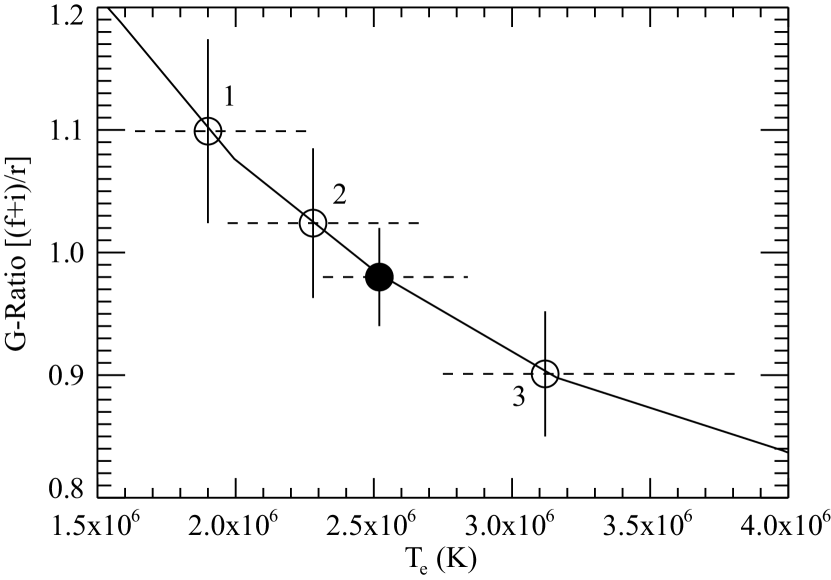
Figure 1: Theoretical G-ratio (i.e., ratio of forbidden plus intercombination to resonance line fluxes) for Ne IX as a function of $T_{e}$ (solid curve) from AtomDB (Foster et al. 2012; Chen et al. 2006). Overplotted are the observed ratios with 1$\sigma$ errors (vertical error bars) for the individual observations (open circles, numbered in time order) and for the summed spectrum (solid circle). Horizontal error bars (dashed lines) show how the errors on the observed ratios translate to the errors on $T_{e}$.

The He-like Ne IX system provides line ratio diagnostics for $T_{e}$, $n_{e}$, and $N_{H}$ (Paper I). Fortunately, the atomic data for this ion are now accurate for diagnostic studies (Chen et al. 2006). Figure 1 shows the theoretical $T_{e}$-dependent curve for Ne IX (Foster et al. 2012) with the measured G-ratios [(forbidden plus intercombination)/resonance] overplotted. During the third observation $T_{e}$ is significantly higher than during the first two observations. This change in $T_{e}$ provides one of the primary motivations for this study.

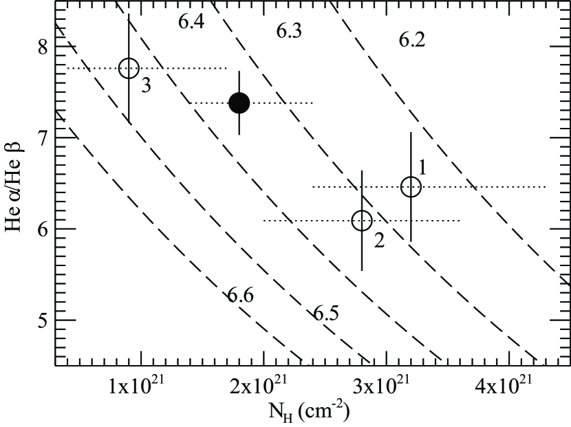
Figure 2: Ratio of the flux of the resonance line (He$\alpha$) to that of He$\beta$ as a function of hydrogen column density (dashed curves), for given log [$T_{e}$] (K) from 6.2 to 6.6 as labeled. Absorption models are from Morrison & McCammon (1983) and line emissivities are from Foster et al. (2012). Overplotted are the observered ratios with 1$\sigma$ errors (vertical error bars) for the individual observations (open circles, numbered in time order) and for the summed spectrum (solid circle). Observed points are placed on the curve appropriate for their $T_{e}$ as determined from their G-ratios. Horizontal error bars (dotted lines) show how the errors both on the observed He$\alpha$/He$\beta$ ratios and on $T_{e}$ (determined from the G-ratios) translate to the errors on $N_{H}$.

The observed Ne IX series ratios rule out resonance scattering, consistent with the measured line broadening (Paper I). The line optical depth is reduced by two orders of magnitude due to the modeled filling factor (Table 2) and turbulent broadening. Figure 2 shows $N_{H}$ inferred from the measured Ne IX resonance He$\alpha$ ($\lambda$13.45) /He$\beta$ ($\lambda$11.54) ratios, using a neutral to near-neutral photoelectric absorber. $N_{H}$ is smaller in the third observation compared with the first two, providing additional motivation for this study. To derive $N_{H}$ from the He$\alpha$/He$\beta$ line ratio, the $T_{e}$-dependence is first determined from the observed G-ratio. Theoretical curves of He$\alpha$/He$\beta$ are then plotted as functions of $N_{H}$, for different values of $T_{e}$ ranging from 1.6 to 4.0 MK. Table 2 gives the derived values for $T_{e}$, $N_{H}$, and $n_{e}$. We note that $n_{e}$ derived from the R-ratio (forbidden/intercombination; not shown) is only marginally significantly different in the third pointing. Since the values of $n_{e}$ from all three pointings are more than an order of magnitude higher than observed from purely coronal sources at Ne IX temperatures (Sanz-Forcada et al. 2003), the assumption that Ne IX forms primarily in the accretion shock remains justified.

Fe XVII also originates primarily in the shock (Paper I). We use the observed $\lambda$15.01 (“3C”) to $\lambda$15.26 (“3D”) line ratios to obtain $T_{e}\approx$ 3.0, 2.1, and 4.6  MK for pointings 1, 2, and 3, respectively. The temperature sensitivity of 3C/3D arises from an inner shell Fe XVI line blend with 3D (Brown et al. 2001). While these $T_{e}$ values are not entirely consistent with those from Ne IX, they support the trend for higher $T_{e}$ during the third pointing. Notably, the ratio for the third observation is consistent with the absence of Fe XVI, as expected at the higher temperature.

We can test the overall consistency of the derived parameters by comparing the observed line fluxes with predictions. For a single component model, the observed line intensity $I_{obs}=W_{\lambda}~{}A~{}\varepsilon(T_{e})~{}EM/(4\pi R^{2})$, where $W_{\lambda}$ is the wavelength-dependent transmission through the absorber (Morrison & McCammon 1983; Wilms et al. 2000), $A$ is the relative elemental abundance, $\varepsilon$ is the emissivity from AtomDB (Smith et al. 2001; Foster et al. 2012), $EM$ is the emission measure ($EM=n_{e}^{2}V$, where $V$ is the volume) and $R$ is the distance to the source. The absorption model assumes solar abundances, which could introduce an error as large as a factor of two in $N_{H}$.

We use the summed observation to determine $A$ and then predict fluxes for the three pointings. Abundance ratios for oxygen, magnesium, and iron compared to neon are in the range of relative abundances found in Paper I. The observed fluxes of Ne IX $\lambda$13.45 along with the values of $n_{e}$, $T_{e}$, and $W_{\lambda}$ determined from the Ne IX diagnostics, give $V$ for each pointing. The predicted fluxes of the resonance lines Mg XI $\lambda$9.17, O VIII $\lambda$18.97 and Fe XVII $\lambda$15.01 are reasonably consistent with observations; however, the observed fluxes show smaller differences than predicted. For all three ions, a smaller difference in the transmission $W_{\lambda}$ gives better agreement. For example, decreasing $N_{H}$ from $\sim 3.0\times 10^{21}$ cm^-2 to $\sim 2.2\times 10^{21}$ cm^-2 brings the O VIII line for the first two pointings into good agreement, while increasing $N_{H}$ from 0.9 $\times 10^{21}$ cm^-2 to a value between 1.0 and 1.3 $\times 10^{21}$ cm^-2 brings the line fluxes for all three ions into excellent agreement for the third pointing. The consistency for Mg XI and Fe XVII is somewhat worse for the first two pointings, probably because their emissivity functions are steeply dropping at such low $T_{e}$. Given order of magnitude differences in emissivities and transmission over the range in $T_{e}$ and $N_{H}$, the good agreement among the different shock diagnostics is remarkable.

We predict Ne X Ly$\alpha$ in a similar manner. Our predictions are low by a factor of ten for the first two pointings, but by only a factor of two for the third. Ne X arises primarily from the corona, but has a larger accretion contribution during the third pointing compared with the other two.

3 Determining the Parameters of the Accretion Shock

The observed variation of $N_{H}$ provides new support for the idea that the accreting pre-shock stream is the absorber of the shocked, X-ray emission (e.g. Lamzin 1999; Gregory et al. 2007; Paper I), since other potential sources of absorption (e.g. interstellar, circumstellar) are not expected to vary significantly. Moreover, the nearly face-on view of the TW Hya system makes the disk itself an implausible absorber. To explore what the pre-shock gas as absorber implies about the geometry of the system, we use the strong shock condition to obtain the electron density of the pre-shock gas ($n_{e}$/4) from the observed density $n_{e}$ of the shock. We assume the observed column density $N_{H}$ is through the same pre-shock gas, and estimate the path length $<l>=4N_{H}/n_{e}$. From Ne IX, $N_{H}=1.8\times 10^{21}$ cm^-2 and $n_{e}=3.2\times 10^{12}$ cm^-3, and thus $<l>=2.2\times 10^{4}$ km. This path length is much smaller than the stellar radius, and thus geometrical effects due to the curvature of the accretion column are insignificant. This estimate of $<l>$ is also an order of magnitude larger than the length of the post-shock cooling zone (derived in Paper I). Absorption by the cooling column appears to be ruled out. Absorption by intervening stellar atmosphere cannot be ruled out, although recent hydrodynamic models produce an “observable” shock in the upper chromosphere for conditions similar to those of TW Hya (Sacco et al. 2008; 2010). Thus we proceed with the assumption that the pre-shock stream is the only absorber.

In the standard model of magnetospheric accretion (Calvet & Gullbring 1998; Günther et al. 2007), the shock temperature can only vary if the accreting material originates at different distances from the star. Königl (1991) gives an expression for the inner truncation radius of the disk that depends only on the mass accretion rate $\dot{M}_{\rm acc}$ and the surface poloidal magnetic field strength $B_{\ast}$, in addition to the stellar mass $M_{\ast}$ and radius $R_{\ast}$. Thus the observed changes in $T_{e}$ indicate variations in $\dot{M}_{\rm acc}$, $B_{\ast}$, or both.

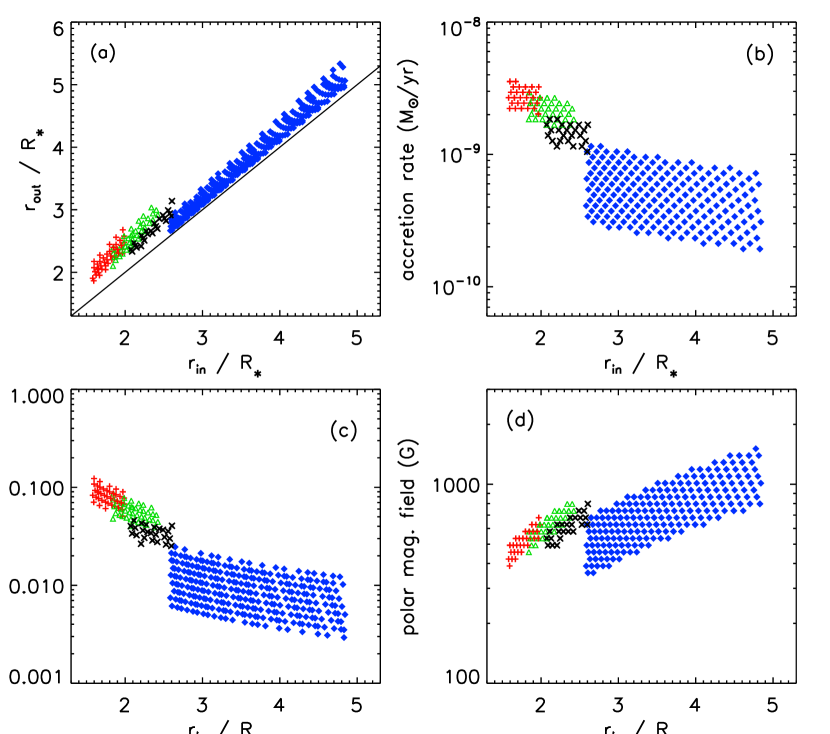
Figure 3: Parameter ranges for the dipole accretion model, constrained by Ne IX diagnostics from time segments 1 (JD 48.0; red crosses), 2 (JD 58.5; green triangles), 3 (JD 61.2; blue diamonds), and the summed data (black X’s). The model parameters plotted vs the inner disk radius are outer disk radius (a), mass accretion rate (b), filling factor at the stellar surface (c), and polar magnetic field at the star (d).

Together $T_{e}$, $n_{e}$, and $N_{H}$ constrain the fundamental parameters of the standard accretion model, namely $\dot{M}_{\rm acc}$, $B_{\ast}$, and filling factor $f$. We assume a solar-type magnetic dipole, aligned with the rotation axis of the star (Cranmer 2008, 2009). Material originates in the gaseous accretion disk between the inner truncation radius $r_{in}$ and an outer radius $r_{out}$, both of which are dependent variables in the model. The accretion stream shocks near the surface of the star, forming a circumstellar ring at a latitude determined by the dipole field geometry and $r_{in}$. We have run a cube of $50\times 50\times 50$ models, independently varying $\dot{M}_{\rm acc}$, $B_{\ast}$, and $f$ for comparison with observations. The value of $\dot{M}_{\rm acc}$ is calculated for the whole star, i. e. in the pole-on case the model accretion rate is twice what we observe. The model parameters are given in Table 2 and illustrated in Figure 3 for the case where the free fall velocity is calculated from $r_{in}$. Similar results are found if we compute the free fall velocity as the square root of the product of the velocities derived from material released at the inner and outer edges of the disk, respectively.

We illustrate the model constraints using the diagnostic lines of Ne IX, since Ne IX is the only He-like ion that produces lines strong enough to determine $T_{e}$, $n_{e}$, and $N_{H}$ from the accretion shock in all three pointings. For the summed data and for each pointing, approximately 100 models, or 0.1% of the 125,000 models computed, are found to agree to within 1$\sigma$ of the derived $T_{e}$, $n_{e}$, and $N_{H}$. The summed spectrum, gives the average values $\dot{M}_{\rm acc}=1.5\times 10^{-9}$ M_⊙ yr^-1, $B_{\ast}=600$ G, and $f=3.5$%. The accreting material originates at $<3R_{\ast}$.

Here we have assumed a single $T_{e}$ and $n_{e}$ model for the shock. In Paper I we found $f$ = 1.1% and $\dot{M}_{\rm acc}$ = $4\times 10^{-10}$ M_⊙ yr^-1 by computing $T_{e}$, $n_{e}$ and the resulting line emission as functions of depth in the post-shock cooling zone, and assuming a truncation radius of 4.5 $R_{\ast}$. We then integrated the emission over the cooling zone and compared to diagnostic line fluxes from the summed spectrum. The shock front temperature was 3.4 MK, compared with 2.5 MK here, while the shock-front electron density was slightly smaller at $2.3\times 10^{12}$ cm^-3. The higher accretion rate derived here arises primarily from the three times larger $f$, with somewhat larger $n_{e}$ offset by somewhat smaller $T_{e}$.

We compare the derived $\dot{M}_{\rm acc}=1.5\times 10^{-9}$ M_⊙ yr^-1 to $0.4$, $1.3$, and $5\times 10^{-9}$ M_⊙ yr^-1, from Muzerolle et al. (2000), Donati et al. (2011), and Batalha et al. (2002), respectively. Curran et al. (2011) report consistent rates from optical diagnostics. Our value agrees well with these estimates. Donati et al. (2011) demonstrate using spectropolarimetric signatures that a strong quadrupole magnetic field (2.5 to 2.8 kG) dominates the magnetic structure in the photosphere of TW Hya; they also report a weaker dipole component (400 to 700 kG) which is capable of disrupting the accretion disk at 3 to 4 $R_{\ast}$, also consistent with our results. Several authors report significantly lower mass accretion rates from X-ray observations: $1.8\times 10^{-10}$ (Curran et al. 2011); $2\times 10^{-11}$ (Stelzer & Schmitt 2004); $2\times 10^{-10}$ (Günther et al. 2007); and, $6$ to $7\times 10^{-11}$ (Günther 2011) M_⊙ yr^-1. All of these studies use a lower $N_{H}$ value determined from global fits to the spectra, accounting for a factor of three or larger difference between their accretion rates and ours. The remaining differences may be due to differences in absolute abundances, filling factors, or relative accretion and coronal contributions to the spectrum, and to different spectra and methods.

The accretion parameters derived from the third pointing are strikingly different from those derived from the first two pointings. $\dot{M}_{\rm acc}$ drops by a factor of 5 while $f$ is smaller by a factor of 7. The truncation radius moves farther out by about 70%. While the derived $r_{in}$ values may be underestimated by the single component shock, $r_{in}$ cannot be too large or the shock temperature would not show any measurable variation. Accounting for the systematic bias introduced by the single component simplification suggests an average $r_{in}$ value of 4 $R_{\ast}$ from the summed spectrum, with a range from 3.4 to 6.1 $R_{\ast}$ for the three pointings.

The large variations in $\dot{M}_{acc}$ and $f$ are unlikely to be the result of rotation or viewing angle, and thus it appears that the accretion rate changes substantially while the stellar magnetic field changes only slightly, if at all. The single spectrum obtained with the MIKE double-echelle spectrograph on Magellan during the third Chandra pointing (Dupree et al. 2012) shows a decrease in the average blue veiling to $r=0.8$ from earlier values of $r>1.2$ during the second Chandra pointing, consistent with a decrease in the accretion rate. The values of $\dot{M}_{\rm acc}$ from the three pointings, 2.8, 2.2, and $0.53\times 10^{-9}$ M_⊙ yr^-1, are all well within the literature values, suggesting that at least some of the differences in the literature are due to intrinsic variability rather than to differences in measurement method. The observations indicate that at lower accretion rates, the stellar magnetic field exerts stronger control of the gas, producing a smaller hot spot at higher latitude, as expected.

Episodic events at lower latitudes occur in the data of Donati et al. (2011), but on time-scales much shorter than the time-resolution of the X-ray spectroscopy. Veiling and spectral line diagnostics for both accretion and wind showed variability during ground-based observations contemporaneous with the Chandra observations (Dupree et al. 2012). The time resolution of these variation signatures is of the order of several minutes, again much shorter than the effective time resolution of the X-ray spectroscopy. X-ray light curves derived from accretion lines show variability on timescales of a few ks (see also Paper I), although these variations are not correlated with the optical photometry, and an enhanced accretion event (during pointing 2) is followed by systematic changes in the optical emission lines (Dupree et al. 2012). A decrease in the accretion rate leads to a complex response by the X-ray light curve: a decrease in intrinsic emission measure is countered by an increase in observed flux due to a decrease in the soft X-ray absorption by the accreting column itself.

4 Conclusions

Significant variability in X-ray accretion diagnostics occurs during the Chandra HETG observations of TW Hya. In particular, variability of the column density $N_{H}$ implicates the pre-shock accreting gas as the X-ray absorber. $N_{H}$ and $n_{e}$ measurements from He-like Ne IX lines support an absorbing path length short compared to the stellar radius but long compared to the shock cooling depth. With $T_{e}$, $n_{e}$, and $N_{H}$ together the X-ray data constrain all the fundamental parameters of the standard accretion model, namely $\dot{M}_{\rm acc}$, $B_{\ast}$, and $f$.

The resulting average mass accretion rate during the Chandra observation, $\dot{M}_{\rm acc}=1.5\times 10^{-9}$ M_⊙ yr^-1, based on Ne IX diagnostics alone, agrees well with optical and ultraviolet techniques. The observations indicate that the mass accretion rate decreases by a factor of 5 during one pointing of $\sim$150 ks, compared with two others. This accretion rate variation appears to arise from changes in the inner radius of the accretion disk.

Table 1: Emission Line Fluxes

Ion	$\lambda_{ref}$	Flux (uncorrected for absorption)
	(Å)	(10-6 ph cm-2 s-1)
		Pointing 1	Pointing 2	Pointing 3
Mg XI	9.17	2.5 $\pm$ 0.4	1.7 $\pm$ 0.5	2.4 $\pm$ 0.4
Ne X	9.71	1.8 $\pm$ 0.8	3.1 $\pm$ 0.5	2.8 $\pm$ 0.6
Ne X	10.24	7.0 $\pm$ 0.7	9.0 $\pm$ 2.0	8.7 $\pm$ 0.8
Ne IX	11.00	7.3 $\pm$ 0.7	6.6 $\pm$ 1.0	7.9 $\pm$ 1.0
Ne IX	11.54	19.9 $\pm$ 1.5	23.7 $\pm$ 1.8	24.2 $\pm$ 1.6
Ne X	12.13	63.8 $\pm$ 3.1	74.1 $\pm$ 3.3	77.2 $\pm$ 3.4
Fe XVII	12.27	3.2 $\pm$ 0.8	4.7 $\pm$ 1.0	2.1 $\pm$ 0.6
Ne IX	13.45	128.3 $\pm$ 6.9	144.7 $\pm$ 7.0	187.8 $\pm$ 8.0
Ne IX	13.55	93.5 $\pm$ 5.5	97.8 $\pm$ 5.9	115.4 $\pm$ 6.2
Ne IX	13.70	47.4 $\pm$ 4.0	50.4 $\pm$ 3.4	53.9 $\pm$ 4.3
Fe XVII	15.01	28.6 $\pm$ 3.5	29.2 $\pm$ 3.5	43.4 $\pm$ 4.1
Fe XVII	15.26	11.7 $\pm$ 2.5	15.0 $\pm$ 3.2	15.8 $\pm$ 2.4
O VIII	16.01	27.1 $\pm$ 3.2	24.3 $\pm$ 3.8	32.7 $\pm$ 3.9
Fe XVII	16.78	25.6 $\pm$ 4.7	22.4 $\pm$ 4.0	25.3 $\pm$ 4.3
Fe XVII	17.05	25.5 $\pm$ 7.6	28.4 $\pm$ 4.5	31.8 $\pm$ 4.3
Fe XVII	17.10	23.0 $\pm$ 6.4	28.7 $\pm$ 4.6	29.4 $\pm$ 4.2
O VIII	18.97	201.3 $\pm$ 15.	210.1 $\pm$ 15.	201.0 $\pm$ 16.

Table 2: Physical Conditions and Accretion Model Parameters

Parameter	Pointing 1	Pointing 2	Pointing 3	Total
$T_{e}$ (MK)	1.9${}^{+0.4}_{-0.3}$	2.3${}^{+0.4}_{-0.3}$	3.1${}^{+0.7}_{-0.4}$	2.5${}^{+0.3}_{-0.2}$
$n_{e}$ (1012 cm-3)	3.0${}^{+0.4}_{-0.3}$	3.1${}^{+0.3}_{-0.3}$	3.9${}^{+0.3}_{-0.4}$	3.2${}^{+0.2}_{-0.2}$
$N_{H}$ (1021 cm-2)	3.2${}^{+1.1}_{-0.8}$	2.8${}^{+0.8}_{-0.8}$	0.9${}^{+0.8}_{-0.5}$	1.8${}^{+0.6}_{-0.4}$
$\dot{M}_{\rm acc}$ (10-9 M⊙ yr-1)	2.78 (2.02–3.56)	2.19 (1.68–2.95)	0.53 (0.19–1.15)	1.45 (1.05–1.84)
Poloidal $B_{\ast}$ ($G$)	523. (389.–679.)	628. (456.–797.)	770. (359.–1510.)	614. (494.–797.)
Filling Factor (%)	8.19 (5.08–12.3)	5.69 (3.91–8.63)	0.95 (0.29–2.46)	3.46 (2.52–4.59)
rin/R∗	1.77 (1.58–1.99)	2.11 (1.84–2.42)	3.60 (2.58–4.89)	2.34 (2.07–2.60)
rout/R∗	2.23 (1.86–2.67)	2.57 (2.10–3.04)	3.82 (2.67–5.33)	2.68 (2.33–3.14)
Latitude	44.6$\arcdeg$	49.0$\arcdeg$	58.7$\arcdeg$	50.8$\arcdeg$