A Nonlinear Force-Free Magnetic Field Approximation Suitable for Fast Forward-Fitting to Coronal Loops. III. The Free Energy

Abstract

An analytical approximation of a nonlinear force-free magnetic field (NLFFF) solution was developed in Paper I, while a numerical code that performs fast forward-fitting of this NLFFF approximation to a line-of-sight magnetogram and coronal 3D loops has been described and tested in Paper II. Here we calculate the free magnetic energy $E_{\rm free}=E_{\rm N}-E_{\rm P}$, i.e., the difference of the magnetic energies between the nonpotential field and the potential field. A second method to estimate the free energy is obtained from the mean misalignment angle change $\Delta\mu=\mu_{\rm P}-\mu_{\rm N}$ between the potential and nonpotential field, which scales as $E_{\rm free}/E_{\rm P}\approx\tan^{2}{(\Delta\mu)}$. For four active regions observed with STEREO in 2007 we find free energies in the range of $q_{\rm free}=(E_{\rm free}/E_{\rm P})\approx 1\%-10\%$, with an uncertainty of less than $\pm 2\%$ between the two methods, while the free energies obtained from 11 other NLFFF codes exhibit a larger scatter of order $\approx\pm 10\%$. We find also a correlation between the free magnetic energy and the GOES flux of the largest flare that occurred during the observing period, which can be quantified by an exponential relationship, $F_{\rm GOES}\propto\exp{(q_{\rm free}/0.015)}$, implying an exponentiation of the dissipated currents.

1 Introduction

The free magnetic energy is the maximum amount of energy that can be released in an active region of the solar corona, such as during a solar flare, a filament eruption, or a coronal mass ejection (CME). Thus, it is important to design reliable methods and tools that can calculate the amount of free energy in order to quantify the energy budget in a catastrophic energy release event, as well as for estimating upper limits in forecasting individual events in real-time. Traditionally, the free energy is calculated by computing the nonpotential field ${\bf B}_{\rm N}({\bf x})$ with a numerical nonlinear force-free field (NLFFF) code and a potential field ${\bf B}_{\rm P}({\bf x})$ for the same photospheric boundary data ${\bf B}(x,y,z_{\rm phot})$, so that the difference of the magnetic field energy density integrated over a volume $V$ encompassing the active region of interest can be quantified as

$$E_{\rm free}={1\over 8\pi}\left(\int{\bf B}_{\rm N}^{2}({\bf x)}\ dV-\int{\bf B}_{\rm P}^{2}({\bf x)}\ dV\right)\ .$$ (1)

This standard method may not necessarily reflect the correct amount of maximum free energy released during a solar flare, since the magnetic field in the photospheric boundary ${\bf B}(x,y,z_{\rm phot})$ may change during a flare (e.g., see measurements by Wang et al., 1994, 2002, 2004, 2013; Wang, 1997, 2006; Wang and Liu, 2010). Another problem with NLFFF codes using the photospheric vector field is the non-force-freeness of the lower chromosphere (Metcalf et al., 1995; DeRosa et al., 2009), which however, can be ameliorated by preprocessing the magnetic boundary data, using chromospheric field measurements (e.g., Metcalf et al., 2005; Jing et al., 2010), or by a multigrid optimization that minimizes a joint measure of the normalized Lorentz force and the divergence of the magnetic field, as proposed by Wiegelmann (2004) and applied by Jing et al., (2009). A quantitative comparison of NLFFF computation methods, however, revealed a substantial scatter of free energies in the order of $\approx\pm 10\%$ (of the potential energy), depending on the numeric code, the boundary specifications, and the spatial resolution (Schrijver et al., 2006; DeRosa et al., 2009). Alternatively, some studies show that the free energy is better estimated by the minimum-energy state above the linear force-free field with the same magnetic helicity (Woltjer, 1958; Régnier and Priest, 2007). Since NLFFF calculations are rather computing-intensive for forward-fitting tasks to coronal constraints, which requires many iterations (for an overview and discussion of different numerical methods see recent reviews by Aschwanden (2004) or Wiegelmann and Sakurai (2012)) or faster non-numerical methods are desirable. Some proxy of the active region’s free magnetic energy has been defined based on the twist and magnetic field orientation near the neutral line (e.g., Falconer et al., 2006, 2011).

Free magnetic energies have been calculated for a variety of solar phenomena, for instance for the evolution of the free magnetic energy during flux emergence and cancellation, using NLFFF codes (e.g., Fang et al., 2012), for the evolution of active regions (e.g., Kusano et al., 2002), for helmet-shaped streamer configurations (Choe and Cheng, 2002), or for breakout CMEs, using MHD simulations (e.g., DeVore and Antiochos, 2005). Theoretical studies quantify the evolution of free magnetic energy for dipolar (Régnier, 2009) and quadrupolar magnetic configurations with a null-point, using different force-free models (Régnier, 2012).

An analytical approximation of a nonlinear force-free magnetic field (NLFFF) solution was developed in Paper I (Aschwanden, 2012), while a numerical code that performs fast forward-fitting of this NLFFF approximation to coronal 3D loops and a line-of-sight magnetogram has been described and tested in Paper II (Aschwanden and Malanushenko, 2012). In this Paper III of the series we are concerned with the calculation of the free energy, generally defined by the difference of the magnetic energies between the nonpotential field and the potential field (Equation (1)). We calculate free energies from simulated data (from Paper II), from the analytical NLFFF solution of Low and Lou (1990), from active region NOAA 10930 during an X3.4 flare modeled by Schrijver et al., (2008) and Malanushenko et al., (2012), and from stereoscopically triangulated loops observed with STEREO (Aschwanden et al., 2012). Section 2 describes the analytical treatment, Section 3 the application to simulated datasets and observations, Section 4 contains a discussion, and Section 5 the conclusions.

2 Analytical Formulation

2.1 The NLFFF Approximation

In Paper I (Aschwanden, 2012) we derived an analytical approximation of a nonlinear force-free field (NLFFF) solution, which fulfills Maxwell’s divergence-free equation ($\nabla\cdot{\bf B}=0$) and the force-free equation $(\nabla\times{\bf B})=\alpha({\bf x}){\bf B}$ with second-order accuracy (of the force-free parameter $\alpha$). The analytical approximation can be specified by a radial field $B_{r}$ and an azimuthal field component $B_{\varphi}$,

$$B_{r}(r,\theta)=B_{j}\left({d^{2}\over r^{2}}\right){1\over(1+b^{2}r^{2}\sin^{2}{\theta})}\ ,$$ (2)

$$B_{\varphi}(r,\theta)=B_{j}\left({d^{2}\over r^{2}}\right){br\sin{\theta}\over(1+b^{2}r^{2}\sin^{2}{\theta})}\ ,$$ (3)

$$B_{\theta}(r,\theta)\approx 0\ ,$$ (4)

$$\alpha(r,\theta)\approx{2b\cos{\theta}\over(1+b^{2}r^{2}\sin^{2}{\theta})}\ ,$$ (5)

where ($r,\varphi,\theta$) are the spherical coordinates of a single magnetic field component ($B_{j},x_{j},y_{j},z_{j},b_{j})$ with a unipolar magnetic charge $B_{j}$ that is buried at position ($x_{j},y_{j},z_{j})$, has a depth $d=1-[x_{j}^{2}-y_{j}^{2}-z_{j}^{2}]^{1/2}$, a vertical twist $\alpha=2b_{j}$, and $r=[(x-x_{j})^{2}+(y-y_{j})^{2}+(z-z_{j})^{2}]^{1/2}$ is the distance of an arbitrary coronal position $(x,y,z)$ to the subphotospheric location $(x_{j},y_{j},z_{j})$ of the buried magnetic charge. The force-free parameter $\alpha$ is expressed in terms of the parameter $b$, which quantifies the number $N_{\rm twist}$ of full twist turns over a (loop) length $L$,

$$b={2\pi N_{\rm twist}\over L}.$$ (6)

This analytical approximation is divergence-free and force-free to second-order accuracy in the parameter $(b\ r\sin\theta)$, which is approximately proportional to the force-free parameter $\alpha$ as defined by Equation (5).

A general magnetic field configuration can be composed by a superposition of $N_{\rm m}$ twisted magnetic field components,

$${\bf B}_{\rm N}({\bf x})=\sum_{j=1}^{N_{\rm m}}{\bf B}_{j}({\bf x})\ ,$$ (7)

which also fulfils the divergence-free and force-free condition with second-order accuracy in $\alpha$ (or $b$).

2.2 The Free Magnetic Energy of a Single Twisted Component

Let us calculate now the free magnetic energy $dE_{\rm free}({\bf x})$ at location $({\bf x})$ for the field resulting from a single twisted (buried) magnetic charge as defined by Equations (1) to (6). Since the radial $B_{r}$ and azimuthal components $B_{\varphi}$ are always orthogonal to each other (Figure 1), we can calculate the total nonpotential magnetic field strength $B_{\rm N}$ at every given point $(r,\varphi)$ simply from the sum of the squared components $B_{r}$ and $B_{\varphi}$,

$$B_{\rm N}=\left(B_{r}^{2}+B_{\varphi}^{2}\right)^{1/2}=B_{j}\left({d^{2}\over r^{2}}\right){1\over\sqrt{(1+b^{2}r^{2}\sin^{2}{\theta})}}\ ,$$ (8)

while the field strength $B_{\rm P}$ of a potential field corresponds to the radial component $B_{r}$ (of a single buried magnetic charge, Equation (2)),

$$B_{\rm P}=B_{r}=B_{j}\left({d^{2}\over r^{2}}\right){1\over(1+b^{2}r^{2}\sin^{2}{\theta})}\ ,$$ (9)

and thus the free energy $dE_{\rm free}({\bf x})$ is just the magnetic energy associated with the azimuthal field component $B_{\varphi}$, with Equations (8) and (9),

$$dE_{\rm free}{(\bf x})=dE_{\rm N}({\bf x})-dE_{\rm P}({\bf x})={1\over 8\pi}[B_{r}({\bf x})^{2}+B_{\varphi}({\bf x})^{2}]-{1\over 8\pi}B_{r}({\bf x})^{2}={1\over 8\pi}B_{\varphi}({\bf x})^{2}.$$ (10)

This definition of the free magnetic energy $dE_{\rm free}({\bf x})$ fulfills the following conditions:

Figure 1.: Diagram of the nonpotential field vector ${\bf B}_{\rm N}$, which is composed of the two orthogonal components of the azimuthal field vector ${\bf B}_{\varphi}$ and the radial field vector ${\bf B}_{r}$, subtending an angle $\theta$.

1. Positivity constraint: The free energy is positive for every nonpotential field at any location ${\bf x}$, i.e., $dE_{\rm free}({\bf x})>0$, since $B_{\varphi}^{2}({\bf x})\geq 0$ and $dE_{\rm free}({\bf x})\propto B_{\varphi}^{2}({\bf x})$ according to Equation (10).

2. Additivity of energies and orthogonality of magnetic field components:  The nonpotential energy corresponds to the sum of the potential energy and the free energy $dE_{\rm N}({\bf x})=dE_{\rm P}({\bf x})+dE_{\rm free}({\bf x})$ according to Equation (1) and Figure 1. Since the energies scale with the square of the magnetic field components, i.e., $dE_{\rm N}({\bf x})\propto B_{\rm N}({\bf x})^{2}$, $dE_{\rm P}({\bf x})\propto B_{r}({\bf x})^{2}$, and $dE_{\rm free}({\bf x})\propto B_{\varphi}({\bf x})^{2}$, the Pythagoras theorem can be applied and it follows that $B_{r}$, $B_{\varphi}$, and $B_{\rm N}$ form a rectangular triangle, with $B_{\varphi}$ perpendicular to the potential field component $B_{\rm P}=B_{r}$.

3. Positive scaling with force-free parameter: The free energy quantifies an excess of nonpotential magnetic field energy compared with the potential field energy, and thus should have a positive scaling with the force-free parameter $\alpha$. Since the free energy scales proportional to the square of the azimuthal magnetic field component (Equation (10)), we have a positive scaling, which is approximately $dE_{\rm free}({\bf x})\propto b^{2}\propto\alpha^{2}$ (Equations (3) and (5)).

4. Potential field limit: The free energy vanishes asymptotically ($dE_{\rm free}({\bf x})\mapsto 0$) with vanishing force-free parameter $|\alpha|\mapsto 0$ or $|b|\mapsto 0$, with the potential field being the limit, $dE_{\rm N}({\bf x})\mapsto dE_{\rm P}({\bf x})$.

5. Finiteness of nonpotential energy: The total nonpotential magnetic energy integrated over an arbitrary large height $r$ converges to a finite value, $E(r\mapsto\infty)=E_{\rm max}$. We can prove the finiteness of the potential energy for a single magnetic charge, which has a square-dependence of the magnetic field, $B(r)\propto r^{-2}$, yielding a 4th-power dependence of the magnetic energy $dE_{\rm P}(r)\propto B(r)^{2}\propto r^{-4}$, and thus a 3th-power dependence for the integrated magnetic energy, $E_{\rm P,tot}\propto\int dE_{\rm P}(r)dr\propto r^{-3}$. For a finite amount of twist and a finite number of magnetic sources, it can be shown that the integral of the resulting nonpotential energy is also finite.

2.3 The Free Magnetic Energy of Multiple Twisted Components

While the foregoing definition of the free energy is calculated for a single twisted (buried) magnetic charge, how can it be generalized for a superposition of an arbitrary number of magnetic charges, as defined in Equation (7)? The sum of the magnetic field contributions from each buried magnetic charge component ${\bf B}_{j}({\bf x})$ add up to the nonpotential field vector ${\bf B}_{\rm N}({\bf x})$, which can be decomposed into two orthogonal components ${\bf B}_{\parallel}({\bf x})$ and ${\bf B}_{\perp}({\bf x})$ in every point of space $({\bf x})$,

$${\bf B}_{\rm N}({\bf x})=\sum_{j=1}^{N_{\rm m}}{\bf B}_{j}({\bf x})={\bf B}_{\parallel}({\bf x})+{\bf B}_{\perp}({\bf x})\ ,$$ (11)

where the parallel component is aligned with the potential field direction, ${\bf B}_{\parallel}\parallel{\bf B}_{\rm P}$, and the perpendicular component is orthogonal to the potential field direction, ${\bf B}_{\perp}\perp{\bf B}_{\rm P}$. For a single (twisted) magnetic component the parallel component ${\bf B}_{\parallel}$ is identical with the radial component ${\bf B}_{r}$, and the perpendicular component ${\bf B}_{\perp}$ is identical with the azimuthal component ${\bf B}_{\varphi}$ (Figure 1). The three magnetic field components $B_{\parallel}=B_{\rm P},B_{\perp}$, and $B_{\rm N}$ are then associated each with one of the three energy components,

$$\begin{array}[]{ll}dE_{\rm free}({\bf x})&=(1/8\pi)B_{\perp}^{2}({\bf x})\\ dE_{\rm P}({\bf x})&=(1/8\pi)B_{\parallel}^{2}({\bf x})\\ dE_{\rm N}({\bf x})&=(1/8\pi)[B_{\parallel}^{2}({\bf x})+B_{\perp}^{2}({\bf x})]\ .\end{array}$$ (12)

Alternatively, the magnetic energy $dE_{\rm P}({\bf x)}$ of the potential field can be computed by using current-free magnetic field components ($B_{j},x_{j},y_{j},z_{j},b_{j}=0$) straightforward with Equation (1), and the magnetic energy $dE_{\rm N}({\bf x})$ of the non-potential field with the current components ($B_{j},x_{j},y_{j},z_{j},b_{j}\neq 0$) with Equation (1) also, which yields the free energies $(E_{\rm free}=E_{\rm N}-E_{\rm P})$, after volume integration. Both methods are fitting the same line-of-sight component of the photospheric boundary $B_{z}(x,y,z_{\rm phot})$ given by the magnetogram, while the non-potential magnetic field affects the transverse field components $B_{x}(x,y,z_{\rm phot})$ and $B_{y}(x,y,z_{\rm phot})$ that are not used as a boundary condition in our forward-fitting method.

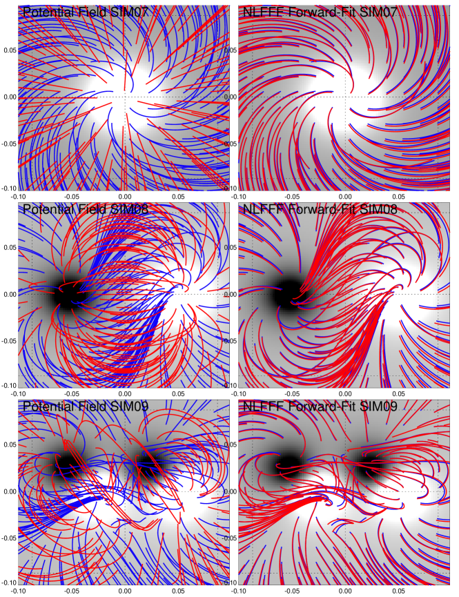
Figure 2.: Forward-fitting of simulated nonpotential field data (cases N7-N9). Each panel shows the line-of-sight magnetogram (grey), simulated coronal loops (the targets of the forward fit) (blue), and magnetic field lines of a theoretical model (red), either the potential field constrained by the line-of-sight magnetogram (left panels), or the forward fit of the NLFFF approximation (right panels).

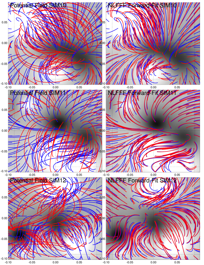
Figure 3.: Forward-fitting of cases N10–N12. Representation similar to Figure 2.

2.4 Free Energy Estimated from Misalignment Angle with Loops

An alternative method is to estimate the free energy in an active region from the misalignment angle $\mu$ between the potential field and the observed coronal loops, or the best-fit nonpotential field. Using the coronal loops as a proxy for the nonpotential field, this would provide a very fast method that requires only the computation of a potential field, supposed we have the 3D coordinates of coronal loops, e.g., from stereoscopic triangulation. Since the mean azimuthal field component is $B_{\perp}=B_{\rm N}\sin{(\Delta\mu)}$ and the mean radial (potential) field component is $B_{\parallel}=B_{\rm N}\cos{(\Delta\mu)}$, the nonpotential energy ratio $q_{\mu}=E_{\rm N}/E_{\rm P}$ follows then directly, using the definition of Equation (11), for the free energy,

$$q_{\mu}={E_{\rm N}\over E_{\rm P}}={B_{\perp}^{2}+B_{\parallel}^{2}\over B_{\parallel}^{2}}=1+\tan^{2}{(\Delta\mu)}\ ,$$ (13)

where the relative misalignment angle $\Delta\mu$ is defined as the difference between the (median) potential $\mu_{\rm P}$ and (median) nonpotential field directions $\mu_{\rm N}$,

$$\Delta\mu=\mu_{\rm P}-\mu_{\rm N}\ .$$ (14)

Ideally, if the NLFFF forward-fitting code matches the coronal loops perfectly (with $\mu_{\rm N}\approx 0$), and thus the relative misalignment angle of the potential field to the loops can be used, $\Delta\mu\approx\mu_{\rm P}$. However, in reality there is always a significant difference between the best-fit NLFFF solution and the observed loop data, either due to stereoscopic measurement errors or due to an additional field misalignment that cannot be described with the particular parameterization of our NLFFF approximation.

3 Numerical Tests and Results

We perform now tests of the calculation of the free magnetic energy using the definitions given in Equations (12) and (13) for four different datasets, using (1) simulated data produced by our analytical NLFFF approximation, (2) the NLFFF solution of Low and Lou (1990) with a known exact analytical solution, (3) active region NOAA 10930 during an X3.4 flare modeled by Schrijver et al., (2008) and Malanushenko et al., (2012), and (4) stereoscopic data from four observed active regions.

3.1 Tests with Simulated Data (P1-N12)

We simulated six cases of potential fields (shown in Figure 3 of Paper II), and six cases with nonpotential fields (Figures 2 and 3), which are similar to the cases N7 to N12 in Paper II, except that we reduced the amount of twist by a factor of five, in order to make them more comparable with observations of real active regions, which have free energies of order $\lower 1.72218pt\hbox{$\;\buildrel<\over{\scriptstyle\sim}\;$}10\%$. We are using the parameterization of our analytical NLFFF approximation, described in Paper I, containing 1, 2, 4, and 10 magnetic source components with variable vertical twist, labeled as cases P1–P6 and N7–N12. We integrate the nonpotential magnetic energy $E_{\rm N}$ in a box that covers the displayed field-of-view centered at the center of the solar disk and has a height range of $h=0.15$ solar radii above the photosphere. The values of the potential energies $E_{\rm P}$ and the ratio of the nonpotential to the potential energy of the model $(q_{\rm model})$, or of the fit ($q_{\rm fit}=E_{\rm N}/E_{\rm P}$), are listed in Table 1. The free energy is $E_{\rm free}=E_{\rm N}-E_{\rm P}=E_{\rm P}(q_{\rm N}-1)$.

Table 1.: Magnetic energy calculations are listed for 20 cases, including six potential-field cases (P1-P6), six nonpotential-field cases (N7-N12), the Low and Lou (1990) case (L1, L2), the Schrijver et al., (2008) case (S1, S2), and four stereoscopically observed active regions (A, B, C, D), specified by the number of magnetic charges $(N_{\rm m})$, the fraction of magnetic energy captured by the model $(q_{E})$, the number of simulated loops $N_{l}$, the potential energy $E_{\rm P}$ (corrected by the factor $q_{E}$), the median misalignment angle $\mu_{\rm P}$ of the potential field, the median misalignment angle $\mu_{\rm N}$ after forward-fitting of the NLFFF model, the predicted energy ratio $q_{\mu}=(1.+\tan^{2}{(\Delta\mu)})$ based on the misalignment angle change $\Delta\mu=\mu_{\rm P}-\mu_{N}$, the forward-fitted nonpotential energy ratio $q_{\rm fit}=E_{\rm N}/E_{\rm P}$, and the volume-integrated nonpotential magnetic energy ratio of the model $q_{\rm model}=E_{\rm model}/E_{\rm P}$, with values computed by Anna Malanushenko (private communication, 2012) using the Low and Lou (1990) data $(^{a})$, the value of 3D-fits labeled as II.b Tables 3 and 4 of Malanushenko et al., (2012) $(^{b})$, and the value of the $Wh^{+}$ code with the smallest misalignment angle $\mu=24^{\circ}$ in Table 1 of DeRosa et al., (2009) $(^{c})$.

Case	$N_{\rm m}(q_{\rm E})$	$N_{\rm loop}$	$\mu_{\rm P}$	$\mu_{\rm N}$	$E_{\rm P}$	$q_{\mu}$	$q_{\rm fit}$	$q_{\rm model}$
					$10^{32}$
					(erg)
P1	1(1.000)	49	0.5	0.0	4.65	1.000	1.000	1.000
P2	2(1.000)	121	1.8	1.2	5.84	1.000	1.000	1.000
P3	4(1.000)	121	2.1	1.4	4.27	1.000	1.000	1.000
P4	10(1.000)	121	2.5	1.3	14.6	1.000	1.000	1.000
P5	10(1.001)	121	3.7	1.4	12.9	1.002	1.000	1.000
P6	10(0.998)	121	3.3	1.9	6.80	1.001	1.000	1.000
N7	1(1.000)	49	18.8	0.2	4.65	1.114	1.010	1.010
N8	2(1.000)	121	10.4	1.2	5.84	1.026	1.009	1.009
N9	4(1.000)	121	13.0	1.8	4.27	1.039	1.016	1.016
N10	10(1.000)	121	17.4	3.1	14.6	1.065	1.082	1.082
N11	10(1.001)	121	17.2	1.1	12.9	1.084	1.113	1.113
N12	10(0.998)	121	25.3	1.9	6.80	1.188	1.163	1.163
L1	100(0.913)	133	14.7	4.8	0.246	1.030	1.023	1.129a
L2	100(0.910)	35	3.9	1.6	0.028	1.002	1.001	1.091a
S1: 2006/12/12	200(0.860)	331	37.3	14.4	18.3	1.179	1.112	$1.21\pm 0.05^{b}$
S2: 2006/12/13	200(0.878)	98	27.3	13.4	17.8	1.061	1.104	$1.08\pm 0.01^{b}$
A: 2007/04/30	100(0.854)	200	23.8	21.4	12.7	1.002	1.006	1.030c
B: 2007/05/09	100(0.807)	70	21.2	17.9	1.08	1.003	1.023
C: 2007/05/19	100(0.784)	100	41.3	22.1	3.47	1.121	1.085
D: 2007/12/11	100(0.810)	87	22.1	14.7	7.83	1.017	1.044

Table 1 demonstrates several results. First, the misalignment angle between the forward-fitted nonpotential field and the simulated loops is in all 12 cases (P1,…,N12) significantly smaller ($\mu_{\rm N}=1.4^{\circ}\pm 0.8^{\circ}$) than the initial potential field misalignment angle $\mu_{\rm P}=9.6^{\circ}\pm 8.5^{\circ}$, which confirms a satisfactory convergence of the forward-fit to the simulated target loops. Second, all ratios of nonpotential to potential energies $E_{\rm N}/E_{\rm P}$ are larger than one, which means that the free energy $E_{\rm free}=E_{\rm N}-E_{\rm P}$ is always positive with our definition given in Equation (12). Third, all 12 simulated cases agree in the nonpotential energy ratio with the simulated input model, i.e., $q_{\rm fit}=q_{\rm model}=E_{\rm N}/E_{\rm P}$ with an accuracy of less than $10^{-5}$, which also confirms the perfect convergence of the forward-fit algorithm. The nonpotential-field cases (N7–N12) have free energies in the range of $q_{\rm fit}=E_{\rm N}/E_{\rm P}=1.010-1.163$, or up to 16% of the potential-field energy, which are also retrieved with an accuracy of better than $10^{-5}$. We compare also the nonpotential energy ratios calculated from the forward-fit ($q_{\rm fit}$) and estimated from the median misalignment angles ($q_{\mu}$; Equation (13)) and find an agreement of $q_{\mu}/q_{\rm fit}=1.02\pm 0.05$ between the two methods.

Figure 4.: Height dependence of the nonpotential energy $E_{\rm N}(h)$ integrated over a volume from height $r=1.0$ to $r=r_{\rm max}$ with $r_{\rm max}=1.15$ solar radii for the six-nonpotential cases (N7–N12 in Table 1). An exponential function is fitted in the upper half height range $r>1.075$ (dotted line).

We test also the finiteness of the nonpotential energy. In Figure 4 we plot the height-integrated total nonpotential energies $E_{\rm N}(r)$ as a function of the height limit $r$ for the six cases N7–N12 (Table 1) and find that each one follows approximately an exponential height dependence (dashed curves in Figure 4),

$$E_{\rm P}(r)\approx E_{\rm max}[1-\exp{(-{r-1\over\lambda})}]\ ,$$ (15)

which has the finite limit $E(r\mapsto\infty)=E_{\rm max}$, and thus confirms the convergence of the code. In our calculations we generally use a height limit of $h_{\rm max}=0.15$ solar radii, which corresponds to about two density scale heights of $T_{\rm e}=1.0$ MK plasma, or four emission measure scale heights.

3.2 Tests of the Low and Lou (1990) NLFFF Solution

An analytically exact solution of a NLFFF model was derived by Low and Lou (1990), described also in Malanushenko, Longcope, and McKenzie (2009). The particular solutions we are using are defined by the parameters (a=0.6, n=2.0) in case L1, and (a=0.01, n=1.0) in the case L2, where $a$ is the Grad-Shafranov constant, $n$ is the harmonic number of the Legendre polynomial, and additional parameters are the depth $l$ of the source below the photosphere and the inclination angle $\phi$ of the axis of symmetry). Forward-fits of our analytical NLFFF approximation to the exact NLFFF solution of Low and Lou (1990) are shown in Figure 5 (top and middle), where we used a computation box of $(100\times 100\times 75)$, with a pixel size of $\Delta x=0.002$ solar radii and a height range of $h_{\rm max}=75\Delta x\approx 0.15$ solar radii. The forward-fit was accomplished by using the line-of-sight magnetogram at a planar surface ($B_{z}(x,y,z=1$) and a set of $N_{l}=133$ (case L1) and $N_{\rm loop}=35$ (case L2) target field lines that mimic coronal loops. The misalignment angle is reduced from $\mu_{\rm P}=14.7^{\circ}$ to $\mu_{\rm N}=4.8^{\circ}$ for case L1, and from $\mu_{\rm P}=3.9^{\circ}$ to $\mu_{\rm N}=1.6^{\circ}$ for case L2, so the forward-fitting reduces the misalignment by about a factor of 3. The resulting nonpotential energy ratios are listed in Table 1, yielding free energies of $2.3\%$ for case L1, and $0.1\%$ for case L2, respectively. These free energies are significantly below the theoretical values calculated in Malanushenko et al., (2009), where values of 13% and 9% are quoted (listed under $q_{\rm model}$ in Table 1), although the misalignment of the forward-fitted field is quite satisfactory. The reasons for the mismatch in the free energy for this particular case is not fully understood, since the convergence behavior of our code seems to be no problem in case of unique solutions (such as the simulated cases N7–N12). We suspect that the parameterization of our NLFFF approximation, which consists of a number of buried point-like magnetic sources, is not adequate or suitable to represent the analytical Low and Low (1990) solution, which consists of extended, smooth magnetic distributions with elliptical shapes, parameterized in terms of Legendre polynomials. It is conceivable that the representation of Legendre polynomials by (spherically symmetric) point sources leads to clustering of closely-spaced point sources with cancelling of the nonpotential (azimuthally twisted) field components.

3.3 Tests of the case of Schrijver et al., (2008)

The magnetic field of active region NOAA 10930, observed with TRACE, Hinode/XRT, and Hinode/SOT on 2006 December 12, 20:30 UT before a GOES-class X3.4 flare (case S1), and on 2006 December 13, 03:40 UT after the flare (case S2), has been extensively modeled with NLFFF codes (Schrijver et al., 2008; Malanushenko et al., 2012). We show a forward-fit of our NLFFF approximation in Figure 5 (bottom panels) to a set of loops (i.e., closed field lines that are randomly chosen from a NLFFF solution computed by Malanushenko et al., 2012). The accuracy of the forward-fitting depends mostly on the number of magnetic field components $N_{\rm m}$, but generally reaches asymptotically a flat plateau for $N_{\rm m}\lower 1.72218pt\hbox{$\;\buildrel>\over{\scriptstyle\sim}\;$}100$ (Aschwanden et al., 2012; Figure 10). For this magnetically very complex active region we needed $N_{\rm m}=200$ magnetic source components to reach the plateau, while $N_{\rm m}\lower 1.72218pt\hbox{$\;\buildrel<\over{\scriptstyle\sim}\;$}100$ was sufficient for all other cases. Here, the median misalignment angle of $\mu_{\rm P}=37.3^{\circ}$ for the potential field was reduced by about a factor of 2.6 to $\mu_{\rm N}=14.4^{\circ}$ for the best-fit nonpotential NLFFF solution (case S1 in Table 1). We measure a potential-field energy of $E_{\rm P}=1.83\times 10^{33}$ erg before the flare (S1), and $E_{\rm P}=1.78\times 10^{33}$ erg after the flare (S2), so a small difference of $\approx 2.6\%$. For the nonpotential magnetic energy ratio we measure $q_{\rm fit}=E_{\rm N}/E_{\rm P}=1.112$ before the flare and $q_{\rm fit}=1.104$ after the flare, and similar values with the misalignment method, i.e., $q_{\mu}=1.179$ and $q_{\mu}=1.061$. Thus the total nonpotential energy decreases by $\Delta E_{\rm N}=0.7\times 10^{32}$ erg ($\approx 5\%$ according to the forward-fit method), or by $\Delta E_{\rm N}=2.7\times 10^{32}$ erg ($\approx 13\%$ (according to the misalignment method).

From the same observing times the free energy ratio was measured with 14 different NLFFF codes in Schrijver et al., (2008; Table 1 therein), which yield energy ratios of $E_{\rm N}/E_{\rm P,free}=1.05\pm 0.05$ before the flare, and $E_{\rm N}/E_{\rm P,free}=1.16\pm 0.14$ after the flare, if we average all methods with equal weight. However, the most reliable NLFFF method among them, according to a quality assessment by visual inspection of five magnetic features seems to be the $Wh^{+}_{pp}$ NLFFF code, which yields an energy ratio of $E_{\rm N}/E_{\rm P,pre}=1.32$ before the flare and $E_{\rm N}/E_{\rm P,pre}=1.19$ after the flare, so a decrease of 13% in the free energy, corresponding to a drop of $\Delta E_{\rm free}\approx 3\times 10^{32}$ erg in free energy, similar to our measurement with the misalignment method ($E_{\rm free}=2.7\times 10^{32}$ erg or 13%). Similarly, Malanushenko et al., (2012; cases with 3D fits labeled as II.b in Table 1 therein) calculates energy ratios of $E_{\rm N}/E_{\rm P}=1.21\pm 0.05$ before the flare and $E_{\rm N}/E_{\rm P}=1.08\pm 0.01$ after the flare, corresponding to a drop of 13% in the free energy.

Thus all three studies agree with a drop in free energy, by an amount of $5\%-13\%$ according to our two methods, versus $\approx 13\%$ for the most reliable NLFFF codes, while lower free energy values and larger misalignment angles result for the other NLFFF codes (Table 1 in Schrijver et al., 2008). Thus our two methods appear to be commensurable with the most reliable NLFFF codes.

3.4 Tests with Stereoscopic Observations

We calculate now the free magnetic energy for four active regions (Table 1) that have all been observed with STEREO and were subjected to previous magnetic modeling, which we label as active regions A, B, C, and D. All four active regions have been subject of potential-field modeling using stereoscopic data, including potential-field stretching (Sandman et al., 2009), buried magnetic charges (Aschwanden and Sandman, 2010), or buried dipoles (Sandman and Aschwanden, 2011), and nonlinear force-free field modeling (Aschwanden et al., 2012).

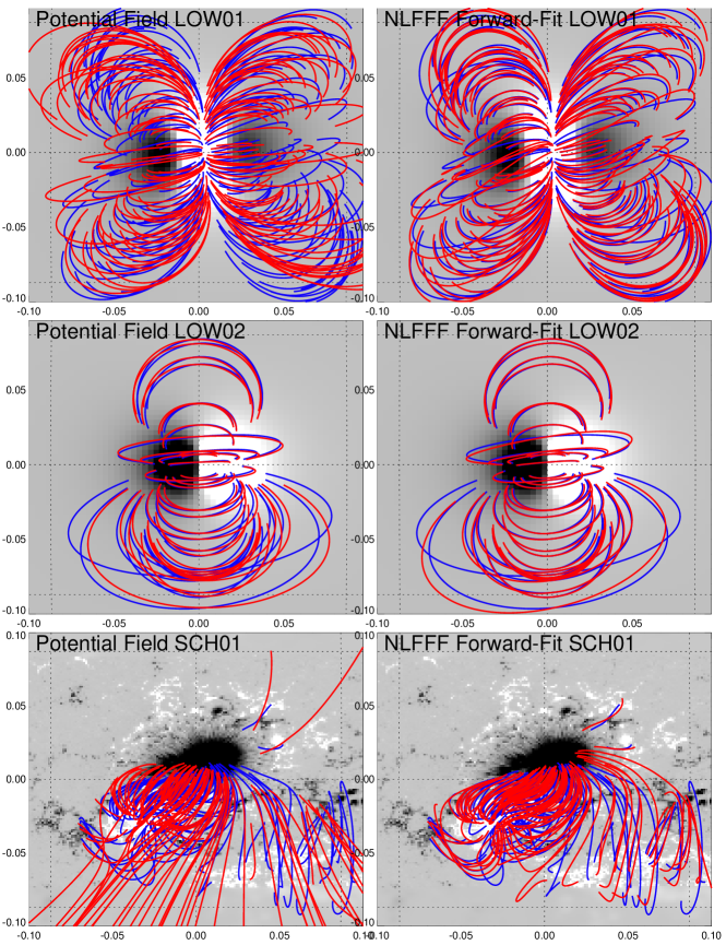
Figure 5.: Forward-fitting of cases L1, L2 (Low and Lou, 1990), and case S1 (Schrijver et al., 2008). Representation similar to Figure 2.

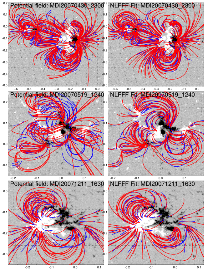
Figure 6.: Forward-fitting of active region cases A (2007 April 30), C (2007 May 19), and D (2007 December 11). Representation similar to Figure 2.

Active region NOAA 10953, 2007 April 30 (A) has been observed during a flare energy build-up phase and a flare trigger by magnetic reconnection at a 3-D null point of a separatrix surface was identified (Su et al., 2009). The magnetic modeling of this active region has been scrutinized with 11 different NLFFF codes, using SoHO/MDI, Hinode/SOT-SP, XRT, and STEREO/EUVI data (DeRosa et al., 2009; Su et al., 2009). For this active region (shown in Figure 6, top panels) we measure a potential field energy of $E_{\rm P}=1.27\times 10^{33}$ erg on 2007 April 30, while Su et al., (2009) measure $E_{\rm P}=0.96\times 10^{33}$ erg on 2007 May 2, which agrees within $\approx 30\%$, over a time difference of two days. For the nonpotential energy ratio we find $E_{\rm N}/E_{\rm P}=1.006$ on 2007 April 30, while Su et al., (2009) find $\approx 1.1$ on 2007 May 2, in the central core of the active region, a few hours before a GOES-class B3.8 and C8.5 flare. Their higher value could thus be attributed to flaring activity. Extensive NLFFF modeling was carried out for 2007 April 30 at 22:24 UT, using Hinode vector magnetograph data (DeRosa et al., 2009). The free energies obtained from 11 different NLFFF codes scatter in the range of $E_{\rm N}/E_{\rm P}=0.87-1.24$, with a value of 1.03 for the $Wh^{+}$ code with the smallest misalignment angle of ($\mu=24^{\circ}$) with respect to the stereoscopically triangulated loops. Including the uncertainties of the boundary conditions in the NLFFF code, a self-consistent NLFFF solution with a nonpotential energy ratio of $E_{\rm N}/E_{\rm P}\approx 1.08$ was obtained, with a potential-field energy of $E_{\rm P}=0.84\times 10^{33}$ erg (Wheatland and Leka, 2011).

Part of the discrepancy could possibly be explained by the different field-of-view, since the Hinode field-of-view used in DeRosa et al., (2009) covers only the central part of the active region, while our field-of-view encompasses the entire active region. Thus we calculated the magnetic energy in the same Hinode field-of-view as used in DeRosa et al., (2009) but find almost identical energy ratios. Our lower value than obtained with the other NLFFF codes could also be attributed to an underestimation of the twist (and thus nonpotential energy) in the core of the active region, where stereoscopic loop triangulation is very sparse due to confusion of loops with “moss” background. If this is true, we generally expect that the avoidance of twisted core structures leads to a stereoscopic undersampling bias, resulting into lower estimates of the free magnetic energy. We also have to keep in mind that the free energy ratio for this active region is the lowest among the four active regions, and thus has the largest relative uncertainty.

Active region NOAA 10953, 2007 May 9 (B) was subject to the first 3D reconstruction with STEREO (Aschwanden et al., 2008a), stereoscopic electron density and temperature measurements (Aschwanden et al., 2008b), and instant stereoscopic tomography and DEM modeling (Aschwanden et al., 2009). This active region exhibits the simplest bipolar magnetic configuration among all four analyzed active regions and we find a nonpotential energy ratio of $E_{\rm N}/E_{\rm P}=1.023$ (Table 3), i.e., a free energy ratio of $\approx 2.3\%$.

Active region NOAA 10953, 2007 May 19 (C) has exhibited multiple filament eruptions in the complex and highly nonpotential magnetic configuration during 2007 May 19 (Li et al., 2008; Liewer et al., 2009; Hara et al., 2011). Some 22 GOES B-class and 2 GOES C-class flares were detected during the observing period (Li et al., 2008). A filament eruption, accompanied by a B9.5 flare, coronal dimming, and and EUV wave was observed and traced with 3D reconstruction after 2007 May 19, 13:00 UT (Liewer et al., 2009). The associated EUV dimming and EUV wave caused by the filament eruption was also analyzed (Attrill et al., 2009). Plasma motion and heating up to $T_{\rm e}=9$ MK was observed for the same flare around 13:00 UT (Hara et al., 2011). For this active region, which we analyzed at 12:47 UT shortly before the flare (shown in Figure 6, middle panels), we found the largest amount of free energy (9%), i.e., a nonpotential energy ratio of $E_{\rm N}/E_{\rm P}=1.085$ (Table 1), which clearly is associated with the filament eruption and flaring activity after 13:00 UT.

Active region NOAA 10978, 2007 December 11 (D) appears also to have a dominant bipolar structure (shown in Figure 6, bottom panels), but some apparent currents along the central neutral line have been modeled with a flux-insertion method (Alex Engell and van Ballegooijen; private communication 2012). For this active region we found a moderate amount of free energy (4%), i.e., a nonpotential energy ratio of $E_{\rm N}/E_{\rm P}=1.044$ (Table 1), which is likely to be stored in the flux rope or filament above the central neutral line.

Figure 7.: GOES soft X-ray light curves of the 0.5-4 Å (upper curve) and 1-8 Å channel (lower curve) during the time of stereoscopic triangulation and magnetic modeling of the four analyzed active regions. The flare peak and preflare background levels are indicated with a step function (thick solid lines). The four active regions are in order of increasing GOES flux (adapted from Aschwanden and Sandman, 2010).

Figure 8.: Correlation between the free energy ratio $q_{\rm free}=E_{\rm free}/E_{\rm P}$ (top panel) or the free energy $E_{\rm free}$ versus the logarithmic (preflare background-subtracted) GOES 0.5-4 Å flux $f_{\rm GOES}$ for active regions A, B, C, and D, are shown, determined with the forward-fit method (diamonds) and with the misalignment method (crosses). Linear regression fits are indicated between linear or logarithmic values are indicated, yielding an exponential function (top panel) or a powerlaw function (bottom panel).

3.5 Correlation of Free Energies with Flare Fluxes

It was noted in earlier work that the level of flaring activity in these four active regions is positively correlated with the nonpotentiality of the magnetic field, evaluated by the average misalignment angle between a magnetic potential-field model and the observed 3D loop coordinates. This correlation was interpreted in terms of a relationship between electric currents and plasma heating (Aschwanden and Sandman, 2010). Since the misalignment angle is a measure of the magnetic nonpotentiality, we expect that there should also be a correlation between the flaring activity level and the free magnetic energy in a flaring active region. The GOES 0.5-4 and 1-8 Å light curves are shown in Figure 7. We plot the (preflare background-subtracted) GOES 0.5-4 Å fluxes $f_{\rm GOES}$ of the largest flare that occurred during the observing period of an active region versus the free energy ratio $q_{B,\rm free}=E_{B,\rm free}/E_{\rm P}$ in Figure 8 (top panel). The preflare background-subtracted GOES fluxes $F_{\rm GOES}$ show a correlation that can be fitted with an exponential function,

$$\left({f_{\rm GOES}\over f_{0}}\right)\approx\exp{\left({q_{\rm free}\over q_{0}}\right)}\ .$$ (16)

with the constants $q_{0}=0.015$ and $f_{0}=10^{-8.4}$ (W m${}^{-2})$. This result implies that the magnitude of the flare (measured here with the GOES soft X-ray flux) is directly related to the free magnetic energy stored in the active region before the flare. If we include the X3.4 GOES flare of AR 10930 (Figure 8, case S1), we see that the observed free energy ratio $q_{\rm fit}=E_{\rm N}/E_{\rm P}-1\approx 0.112$ lies along the same trend of the extrapolated exponential function.

Also the free energy $E_{\rm free}$, an absolute measure of the nonpotential energy, shows a correlation with the observed GOES flux, approximately following a powerlaw (Figure 8, bottom),

$$\left({f_{\rm GOES}\over f_{0}}\right)\approx\left({E_{\rm free}\over E_{0}}\right)^{3}\ .$$ (17)

with the constants $f_{0}=10^{-8.4}$ (W m${}^{-2})$ and $E_{0}=6\times 10^{30}$ erg. Only the active region (B) with the lowest free energy is an outlier to this powerlaw relationship.

4 Discussion

4.1 Accuracy of the Free Energy

Compared with the other (numerical) NLFFF codes, our analytical NLFFF code has the following advantages: (1) computational speed that allows fast forward-fitting to observed coronal data; (2) simplicity of explicit analytical formulation; (3) spherical geometry of solar surface is fully implemented; and (4) the free energy meets the five criteria of positivity, additivity of energy (or orthogonality of magnetic field components), positive scaling with force-free parameter $\alpha$, potential field limit for small $\alpha$’s, and finiteness of nonpotential energy. In this study we calculated the free magnetic energy for four different test datasets and aim to validate the accuracy.

The first test dataset consists of simulated loops, which are analytically defined by the same parameterization as the magnetic field lines that are forward-fitted to the simulated data. We find that the total nonpotential magnetic energies $E_{\rm N}$ are retrieved with an accuracy of $\approx 10^{-5}$ for these cases, and the free energy ratios $E_{\rm N}/E_{\rm P}$ are retrieved with an accuracy of $\approx 10^{-3}$. The high accuracy just confirms the convergence behavior of our code in the case of a unique solution, as it is the case when the forward-fitting model has the same parameterization as the fitted simulation dataset.

The second test dataset consists of an analytical NLFFF solution, which has a completely different parameterization in terms of the Green’s function applied to constant-$\alpha$ point sources (Chiu and Hilton, 1977; Low and Lou, 1990; Lothian and Browning, 1995; Malanushenko et al., 2009, 2011, 2012). The particular case described in Low and Lou (1990) consists of three smooth elliptical magnetic field concentrations and contains an amount of 13% free energy, while we recovered only 2% with the forward-fit. The poor performance is possibly due to the particular topology of the Low and Lou (1990) model, which has extended (elliptical) magnetic field regions parameterized with smooth Legendre polynomials, which cannot be fitted uniquely with spherical point sources. However, because this case is untypical for solar observations, which appear to consist of many small-scale flux concentrations that can be easier fitted with point sources, the accuracy of free energies may be much better for real solar data.

The third data set consists of an observed flaring active region with a large X3.4 flare, for which a NLFFF solution was calculated. For the free energy we obtain a value of order 11%-18% before the flare, which approximately agrees with the most reliable NLFFF solution (16%-32%) computed in Schrijver et al., (2008) and Malanushenko et al., (2012). Also for the sign of the change in nonpotential magnetic energy during this X3.4 flare we obtain the same sign and a similar value for the decrease of free energy ($5\%-13\%$) as the values computed in Schrijver et al., (2008) and Malanushenko et al., (2012), $\approx 13\%$.

The fourth test dataset consists of four solar active regions, for which the 3D coordinates of coronal loops could be stereoscopically triangulated. For these four cases we obtained free energies of 0.6%, 2.3%, 4.4%, and 8.5%. Only for the first case (active region A, 2007 April 30) we have comparisons with other NLFFF codes. The most reliable NLFFF code that exhibits the smallest misalignment angle with stereoscopic loops, yield 3% free energy, which is close to our result of $E_{\rm free}/E_{\rm P}=0.6\%$. The free energy obtained from all 11 NLFFF solutions yields a much larger scatter, i.e., $E_{\rm free}/E_{\rm P}=10\%\pm 12\%$ (Table 1 in DeRosa et al., 2009).

4.2 Scaling Law between Magnetic Energy and Flare Soft X-ray Flux

We found a correlation between the free magnetic energy and the GOES flux of the largest flare that occurred during the observing period (Equation 16). Since our nonpotential field solution is parameterized by a vertical twist of magnetic charges, the free energy is directly proportional to the magnetic energy associated with the azimuthal field component $B_{\varphi}$, and thus approximately proportional to the squared force-free $\alpha$ parameter or the number $N_{\rm twist}$ of twists per length unit, (Equations (10) and (6)),

$$q_{\rm free}({\bf x})={dE_{\rm N}({\bf x})\over dE_{\rm P}({\bf x})}-1={B_{\varphi}^{2}\over B_{r}^{2}}=(br\sin{\theta})^{2}\propto N_{\rm twist}^{2}\propto\alpha^{2}\ .$$ (18)

On the other side, the stress-induced heating rate $E_{\rm H}$ by Ohmic dissipation (or Joule dissipation) is proportional to the square of the currents, (e.g., van Ballegooijen, 1986), which is also proportional to the square of $\alpha$ (with ${\bf j}/4\pi=\nabla\times{\bf B}=\alpha{\bf B}$), and thus to the free energy,

$$E_{\rm H}={j^{2}\over\sigma}\propto{\alpha^{2}B^{2}\over 4\pi\sigma}\ ,$$ (19)

where $\sigma$ is the classical conductivity. Thus we can express Equation (16) in terms of twists, currents, or heating rates,

$$F_{\rm SXR}\propto\exp{(q_{\rm free})}\propto\exp{(N_{\rm twist}^{2})}\propto\exp{(\alpha^{2})}\propto\exp{(j^{2}/B^{2})}\propto\exp{(E_{\rm H}/B^{2})}\ .$$ (20)

Our empirical finding suggests that the energy radiated from the heated plamsa is not just proportional to the heating energy, but “exponentiated” by the current density $j$, the force-free parameter $\alpha$, the number of twists $N_{\rm twist}$, or the heating rate $E_{\rm H}$ of Joule dissipation. This implies a highly nonlinear mechanism that converts vertical twist into thermal radiation via dissipated currents, as envisioned in stress-induced reconnection (Sturrock and Uchida, 1981; Parker, 1983). Our linear regression fit of the free energy versus the GOES flux yields a lower limit of $F_{\rm GOES}=10^{-8.4}$, which corresponds to a GOES-class Z4-event, about the magnitude of the smallest detectable nanoflare. The largest flare among our analyzed cases is an X3.4 GOES-class flare. Apparently, the exponential relationship between soft X-ray flux and free energy discovered here holds even approximately for large GOES X-class flares (Figure 8). The nonlinearity is also reflected by the fact that the thermal energy of the soft X-ray flux is not just proportional to the free magnetic energy, but rather exhibits a highly nonlinear powerlaw function with a powerlaw index of $\approx 3$ (Equation (17)).

5 Conclusions

We calculated the total free magnetic energy contained in a coronal volume encompassing an active region for four different kinds of datasets: (1) simulated data, (2) data created from an analytical NLFFF solution by Low and Lou (1990), (3) a flaring active region, and (4) four active regions observed with STEREO and SOHO/MDI. The free magnetic energy $E_{\rm free}=E_{\rm N}-E_{\rm P}$ is defined by the difference of the nonpotential ($E_{\rm N}$) and the potential magnetic field energy ($E_{\rm P}$). The nonpotential magnetic field ${\bf B}_{\rm N}({\bf x})$ is defined by an analytical approximation of a NLFFF solution that is parameterized by buried magnetic charges with vertical twists (derived in Paper I). The numerical code that performs fast forward-fitting of magnetic field lines to coronal 3D constraints, such as stereoscopically triangulated loops, is described in Paper II, along with the simulated data. Our findings are as follows:

1. A first method to calculate the free energy results from forward-fitting of our analytical NLFFF approximation by associating the perpendicular magnetic field component $B_{\perp}$ with the free energy, $dE_{\rm free}=B_{\perp}^{2}/8\pi$, while the parallel component $B_{\parallel}$ is associated with the potential field energy $dE_{\rm P}=B_{\parallel}^{2}/8\pi$. This definition of the free energy fulfills the conditions of (i) positivity of free energy, (ii) additivity of energies, $E_{\rm N}=E_{\rm P}+E_{\rm free}$ and orthogonality $B_{\perp}({\bf x})\perp B_{\rm P}({\bf x})$, (iii) a positive scaling with the force-free parameter, $dE_{\rm free}\propto\alpha^{2}$, (iv) the potential-field limit, $E_{\rm N}(\alpha\mapsto 0)=E_{\rm P}$, and (v) the finiteness of the nonpotential energy with height $h$, $E_{\rm N}(h\mapsto\infty)=E_{\rm max}$.

2. A second method to estimate the free energy can be obtained from the mean misalignment angle $\Delta\mu=\mu_{\rm P}-\mu_{\rm N}$ between a potential and a nonpotential field (or stereoscopically triangulated coronal loops). The free energy ratio is then $E_{\rm free}/E_{\rm P}\approx\tan^{2}{(\Delta\mu)}$. We find that the uncertainty of this method amounts to $\approx\pm 2\%$ for the nonpotential magnetic energy.

3. Calculating the free energies for the simulated data we find a high fidelity of order $10^{-5}$ in retrieving the free energy, which is due to the fact that the simulated data have the same parameterization as the forward-fitting method, constraining a single best-fit solution.

4. Calculating the free energy for the Low and Lou (1990) analytical case, our NLFFF code finds a significantly lower value than theoretically calculated, probably because of the special morphopology (parameterized with smooth Legendre functions), which cannot adequately be fitted with our NLFFF code that is designed for spherical magnetic point sources, as found in solar magnetograms.

5. Calculating the free energy for observed active regions constrained by the 3D coordinates of stereoscopically triangulated coronal loops, we find free energy ratios of $q_{\rm free}=E_{\rm free}/E_{\rm P}\approx 1\%-10\%$. The uncertainty of the free energy determined with our forward-fitted NLFFF approximation appears to be at least as good as the uncertainty among other (standard NLFFF extrapolation) codes.

6. We find also a correlation between the free magnetic energy $E_{\rm free}$ and the GOES flux of the largest flare that occurred during the observing period, which can be quantified by an exponential relationship, $F_{\rm GOES}\propto\exp{(q_{\rm free})}$, implying an exponentiation of the dissipated currents.

In summary, this study demonstrates that the free energy in active regions can be calculated and predicted with our analytical NLFFF approximation with an accuracy that is commensurable with other standard NLFFF codes. Our code has the additional advantages of computational speed for forward-fitting of coronal data, correct treatment of the curved solar surface, positivity, and finiteness of free energy. In addition, forward-fitting of our NLFFF approximation achieves a significantly smaller misalignment angle with respect to the observed coronal loops ($\mu\approx 2^{\circ}-22^{\circ}$), compared with the results of other NLFFF codes ($\mu=20^{\circ}-44^{\circ}$; DeRosa et al., 2009). The most limiting drawback of our method is the availability of stereoscopic data with suitable spacecraft separation angle (which was most favorable in 2007, the first year of the STEREO mission). In future work we attempt to circumvent the 3D geometry of coronal loops by using only the 2D projections of coronal loops, which can (manually or automatically) be traced from loop-rich EUV or soft X-ray images and do not require stereoscopic data at all.

The author appreciates the provided data and helpful discussions with Anna Malanushenko and Marc L. DeRosa. Part of the work was supported by NASA contract NNG 04EA00C of the SDO/AIA instrument and the NASA STEREO mission under NRL contract N00173-02-C-2035.

References

Aschwanden, M.J.: 2004, Physics of the Solar Corona. An Introduction, Praxis Publishing Co., Chichester UK, and Springer, Berlin, Section 5.3.

Aschwanden, M.J., Wülser, J.P., Nitta, N.V., Lemen, J.R.: 2008a, Astrophys. J. 679, 827.

Aschwanden, M.J., Nitta, N.V., Wülser, J.P., Lemen, J.R.: 2008b, Astrophys. J. 680, 1477.

Aschwanden, M.J., Wülser, J.P., Nitta, N.V., Lemen, J.R., Sandman, A.W.: 2009, Astrophys. J. 695, 12.

Aschwanden, M.J., Sandman, A.W.: 2010, Astronom. J. 140, 723.

Aschwanden, M.J., Wülser, J.P., Nitta, N.V., Lemen, J.R., DeRosa, M.L., Malanushenko, A: 2012, Astrophys. J. 756, 124.

Aschwanden, M.J.: 2012, Solar Phys. (online-first), DOI: 10.1007/s11207-012-0069-7, (Paper I).

Aschwanden, M.J., Malanushenko, A.: 2012, Solar Phys. (online-first), DOI: 10.1007 /s11207-012-0070-1, (Paper II).

Attrill, G.D.R., Engell, A.J., Wills-Davey, M.J., Grigis, P., Testa, P.: 2009, Astrophys. J. 704, 1296.

Chiu, Y.T., Hilton, H.H.: 1977, Astrophys. J. 212, 873.

Choe, G.S., Cheng, C.Z.: 2002, Astrophys. J. Lett. 574, L179.

DeRosa, M.L., Schrijver, C.J., Barnes, G., Leka, K.D., Lites, B.W., Aschwanden, M.J., et al., : 2009, Astrophys. J. 696, 1780.

DeVore, C.R., Antiochos, S.K.: 2005, Astrophys. J. 628, 1031.

Falconer, D., Moore, R., Gary, G.A.: 2006, Astrophys. J. 644, 1258.

Falconer, D., Barghouty, A.F., Khazanov, I., Moore, R.: 2011, Space Weather 9(4), CiteID S04003.

Fang, F., Manchester, W.IV., Abbett, W.P., van der Holst, B: 2012, Astrophys. J. 754 15.

Hara, H., Watanabe, T., Harra, L.K., Culhane, J.L., Young, P.R.: 2011, Astrophys. J. 741, 107.

Jing, J., Chen, P.F., Wiegelmann, T., Xu,Y., Park, S.H., Wang H.: 2009, Astrophys. J. 696, 84.

Jing, J., Tan,C., Yuan, Y., Wang, B., Wiegelmann, T., Xu,Y., Wang H.: 2010, Astrophys. J. 713, 440.

Kusano, K., Maeshiro, T., Yokoyama, T., Sakurai,T.: 2002, Astrophys. J. 577, 501.

Li, Y., Lynch, B.J., Stenborg, G., Luhmann, J.G., Huttunen, K.E.J., Welsch, B.T., Liewer, P.C., Vourlidas, V.: 2008, Astrophys. J. Lett. 681, L37.

Liewer, P.C., De Jong, E.M., Hall, J.R., Howard, R.A., Thompson, W.T., Culhane, J.L., Bone, L., van Driel-Gesztelyi, L.: 2009, Solar Phys. 256, 57.

Lothian, R.M., Browning, P.K.: 1995, Solar Phys. 161, 289.

Low, B.C., Lou, Y.Q.: 1990, Astrophys. J. 408, 689.

Malanushenko, A., Longcope, D.W., McKenzie, D.E.: 2009, Astrophys. J. 707, 1044.

Malanushenko, A., Yusuf, M.H., Longcope, D.W.: 2011, Astrophys. J. 736, 97.

Malanushenko, A., Schrijver, C.J., DeRosa, M.L., Wheatland, M.S., Gilchrist, S.A.: 2012, Astrophys. J. 756, 153.

Metcalf, T.R., Jiao, L., Uitenbroek, H., McClymont, A.N., Canfield, R.C.: 1995, Astrophys. J. 439, 474.

Metcalf, T.R., Leka, K.D., Mickey, D.L.: 2005, Astrophys. J. Lett. 623, L53.

Parker, E.N.: 1983, Astrophys. J. 264, 642.

Régnier, S., Priest, E.R.: 2007, Astron. Astrophys. 669, L53.

Régnier, S.: 2009, Astron. Astrophys. 497, 17.

Régnier, S.: 2012, Solar Phys. 277, 131.

Sandman, A.W., Aschwanden, M.J., DeRosa, M.L., Wülser, J.P., Alexander D.: 2009, Solar Phys. 259, 1.

Sandman, A.W., Aschwanden, M.J.: 2011: Solar Phys. 270, 503.

Schrijver, C.J., DeRosa, M., Metcalf, T.R., Liu, Y., McTiernan, J., Regnier, S., Valori, G., Wheatland, M.S., Wiegelmann,T.: 2006, Solar Phys. 235, 161.

Schrijver, C.J., DeRosa, M., Metcalf, T.R., Barnes, G., Lites, B., Tarbell,T., et al., 2008, Astrophys. J. 675, 1637.

Sturrock, P.A., Uchida, Y.: 1981, Astrophys. J. 246, 331.

Su, Y., Van Ballegooijen, A., Lites, B.W., DeLuca, E.E., Golub, L., Grigis, P.C., Huang, G.,, Ji, H.S.: 2009, Astrophys. J. 691, 105.

Van Ballegooijen, A.A.: 1986, Astrophys. J. 311, 1001.

Wang, H., Ewell, M.W.Jr., Zirin, H.: 1994, Astrophys. J. 424, 436.

Wang, H.: 1997, Solar Phys. 174, 163.

Wang, H., Spirock, T.J., Qiu, J., Ji, H., Yurchyshyn, V., Moon, Y.J., Denker, C., Goode,P.R.: 2002, Astrophys. J. 576, 497.

Wang, H., Qiu, J., Jing, J., Spirock, T. J., Yurchyshyn, V., Abramenko, V., Ji, H., Goode, P.R.: 2004, Astrophys. J. 605, 931.

Wang, H. 2006, Astrophys. J. 649, 490.

Wang, H., Liu,C.: 2010, Astrophys. J. Lett. 716, L195.

Wang, S., Liu, C., Wang, H. 2013, Astrophys. J. Lett. 757, L5.

Wheatland, M.S., Leka, K.D.: 2011, Astrophys. J. 728, 112.

Wiegelmann, T.: 2004, Solar Phys. 219, 87.

Wiegelmann, T., Sakurai T.: 2012, Living Rev. Solar Phys. 9(5), http://solarphysics.livingreviews.org/Articles/lrsp-2012-5.

Woltjer, L.: 1958, Proc. Ntal. Acad. Sci., 44, 489.