Constrained NMSSM with a 126 Higgs boson:
A global
analysis
Abstract
We present the first global analysis of the Constrained NMSSM that investigates the impact of the recent discovery of a 126 Higgs-like boson, of the observation of a signal for branching ratio , and of constraints on supersymmetry from /fb of data accumulated at the LHC, as well as of other relevant constraints from colliders, flavor physics and dark matter. We consider three possible cases, assuming in turn that the discovered Higgs boson is (i) the lightest Higgs boson of the model; (ii) the next-to-lightest Higgs boson; and (iii) a combination of both roughly degenerate in mass. The likelihood function for the Higgs signal uses signal rates in the and channels, while that for the Higgs exclusion limits assumes decay through the , , and channels. In all cases considered we identify the % and % credible posterior probability regions in a Bayesian approach. We find that, when the constraints are applied with their respective uncertainties, the first case shows strong CMSSM-like behavior, with the stau coannihilation region featuring highest posterior probability, the best-fit point, a correct mass of the lightest Higgs boson and the lighter stop mass in the ballpark of 1. We also expose in this region a linear relationship between the trilinear couplings of the stau and the stop, with both of them being strongly negative as enforced by the Higgs mass and the relic density, which outside of the stau coannihilation region show some tension. The second and the third case, on the other hand, while allowed are disfavored by the constraints from direct detection of dark matter and from . Without the anomalous magnetic moment of the muon the fit improves considerably, especially for negative effective parameter. We discuss how the considered scenarios could be tested further at the LHC and in dark matter searches.
1 Introduction
In July 2012 the CMS and ATLAS collaborations at the LHC made the announcement of a discovery of a boson with mass [1] and [2], respectively, consistent with the Higgs boson predicted by the electroweak (EW) Standard Model (SM). The CMS Collaboration has recently updated its results [3] to . The updated result is based on the analysis of the data corresponding to integrated luminosities of 5.1/fb at and up to 12.2/fb at in the , , , and decay channels. The ATLAS analysis combined approximately 4.8/fb of 2011 data at in the same five channels with 5.8/fb of data at in the , and channels only. Evidently, the excess of events near the reported mass is driven by the and channels, owing to the highest mass resolution of these channels. Both collaborations also determined the ratio of the observed Higgs production cross section to the one predicted by the SM, in each of the mentioned Higgs decay channels . An enhancement in the channel was reported by ATLAS, with , as well as by CMS, with . On the other hand, the updated value of by CMS [4] and ATLAS [5] is, within error, SM-like.
While its exact characteristics are still being carefully examined, such a boson is not only consistent with the SM Higgs particle but can also be easily accommodated into models of new physics, particularly those based on softly broken low-energy supersymmetry (SUSY) which actually predict a relatively light Higgs boson. Most studies have been performed within the framework of the two Higgs doublet Minimal Supersymmetric Standard Model (MSSM), usually augmented by various unification boundary conditions. The framework, however, suffers from the so-called “-problem” [6]: the SUSY-preserving parameter in the superpotential is expected to be of the order of the SUSY breaking scale to ensure correct radiative EW symmetry breaking.
Perhaps the most compelling and simplest solution to the -problem is to invoke an additional gauge singlet field coupled to the Higgs doublets of the MSSM [6]. The -term is then generated dynamically through the vacuum expectation value (vev) of the singlet field which is of the order of . The model is commonly referred to as the Next-to-Minimal Supersymmetric Standard Model (NMSSM); for reviews see, e.g., [7, 8]. After the discovery of the Higgs-like boson, numerous studies have appeared in the context of the NMSSM [9, 10, 11, *Cao:2012fz, *Vasquez:2012hn, *Rathsman:2012dp, *Das:2012ys, 16, *Gunion:2012he, 18, *Bae:2012am, *Kang:2012bv, *Cheng:2012pe, *Perelstein:2012qg, *Belanger:2012sd, *Agashe:2012zq, 24, 25, *Belanger:2012tt, *Gogoladze:2012jp, *LopezFogliani:2012yq, 29], since the model presents several interesting features. In the NMSSM the particle content remains the same as in the MSSM, except that the number of Higgs bosons increases from three to five: three neutral scalars and two neutral pseudoscalars . The number of neutralinos also increases from four to five, , owing to the singlino partner of the singlet Higgs boson.
On the phenomenological front, a two-loop theoretical upper bound on the mass of the lightest -even Higgs boson, , can increase by a few GeV compared to the MSSM for some combinations of the model’s parameters. Moreover, in the context of the recent LHC results, the next-to-lightest -even Higgs boson of the model, , could also have mass around 126 with being even lighter than the LEP bound on the SM-like Higgs boson mass, without violating it [9, 10], owing to the singlet-doublet mixing effects. Both features potentially allow us to achieve the correct mass of the experimentally detected Higgs without excessive fine-tuning [30, 31, 32, 33], making the NMSSM potentially a more “natural” model than the MSSM. Finally, the NMSSM also offers the additional possibility that the observed excess in the and rates could be due to the combination of and decays (with and being almost degenerate) [16]. Besides masses, the decay rates of the Higgs boson(s) are also affected by the modifications in the superpotential. For example, for large doublet-singlet mixing, the coupling becomes suppressed, reducing the total decay width. As a result, the branching ratio (BR) of becomes marginally enhanced compared to the SM or the MSSM [34]. An important consequence of this feature is that lighter than 115 could have escaped detection at LEP, and also at the LHC, due to the possibility of its decay into a pair of the two lighter pseudoscalars, (see, e.g., [35]), causing thus a suppression in all of the other BR’s of .
The NMSSM in its most general form contains more than a hundred free parameters: those appearing in the MSSM and some additional ones relating to the extended Higgs sector. Similarly to the MSSM, where imposing universality conditions on the soft SUSY-breaking parameters of the model at the scale of grand unification (GUT scale) leads to the Constrained MSSM (CMSSM) [36], a GUT-constrained version of the NMSSM (CNMSSM) [37, 38, 39] can be defined; see Sec. 2 for more details and discussion.
It is well known that in the CMSSM the lightest Higgs boson’s mass, as calculated at two-loop level with FeynHiggs [40] or SOFTSUSY [41], is typically a few GeV below 126, which can be considered as somewhat unsatisfactory even if one takes into account a residual error of some 2–3 [42] from scheme dependence. (Values of around 126 can still be obtained in the CMSSM for at the expense of increased fine-tuning [43].) A priori one could expect that in the CNMSSM, with more freedom in the Higgs sector, the tension will be reduced. However, recent studies [29] using random scans with fixed-window application of the constraints have shown that in the CNMSSM it is extremely difficult to obtain a Higgs boson as heavy as 126, particularly one with an enhanced decay rate, while also satisfying other phenomenological constraints, thus nullifying the noted advantages of the singlet-extension of the MSSM.
On the other hand, it has been demonstrated by our recent global analysis of the CMSSM [43] and by some earlier Bayesian studies [44, 45] that a proper treatment of the experimental constraints through a likelihood function can lead to significantly different results from “top-hat” scans where such constraints are typically implemented in a more simplified boxlike fashion, with all points accepted when satisfying experimental values within some fixed range (typically within ), and otherwise rejected. One of the main advantages of the statistical approach is that scanned points are instead “weighted” by the total , thus indicating how well they fit all constraints. For example, in the top-hat approach a point giving a value of even one constraint slightly beyond the allowed range while reproducing central values of all the other constraints would be rejected, while a point with values for all the constraints barely within the allowed boxes would be completely allowed. In contrast, in a statistical approach both points would be accepted but weighted with their respective . Another advantage of the statistical approach based on the likelihood function is that theoretical and experimental uncertainties can be easily implemented in a consistent manner. Thanks to some recent developments in sampling algorithms (see, e.g., [46] and [47]), multidimensional Bayesian scans can now be carried out rather quickly and efficiently.
One should note two important changes in the data that have recently taken place on the experimental front. In November 2012 the LHCb Collaboration published the most recent update of their search for the rare decay [48], reporting an excess of candidates over the background. The measured value, , is now very close to the time-averaged SM value, [49, 50]. We include the constraint in our likelihood function taking into account both theoretical and experimental uncertainties, as will be described below.
The other important update was the top pole mass by the Particle Data Group, obtained from an average of data from Tevatron and the LHC at , [51]. As we shall see below this is a welcome increase relative to its previous value in the context of the Higgs sector of constrained SUSY models as it pushes the mass of up, closer to the experimentally observed Higgs-like resonance mass.
In this article, we present the first global Bayesian analysis of the CNMSSM after the observation of the SM Higgs-like boson. We separately consider the cases of this boson being , or , or a combination of both. We test the parameter space of the model against the currently published, already stringent constraints from SUSY searches at the LHC and other relevant constraints from colliders, -physics and dark matter (DM) relic density. Our goal is to map out the regions of the parameter space of the CNMSSM that are favored by these constraints. As in our CMSSM study [43], the CMS razor limit based on of data is implemented through an approximate but accurate likelihood function. We also study the effects of relaxing the constraint.
The article is organized as follows. In Sec. 2 we briefly revisit the model, highlighting some of its salient features. In Sec. 3 we detail our methodology, including our statistical approach and our construction of the likelihoods for the signal, the analysis, and the CMS Higgs searches. In Sec. 4 we present the results from our scans and discuss their novel features. We summarize our findings in Sec. 5.
2 The NMSSM with GUT-scale universality
The NMSSM is an economical extension of the MSSM, in which one adds a gauge-singlet superfield whose scalar component couples only to the two MSSM Higgs doublets and at the tree level.222For simplicity we will be using the same notation for superfields and their bosonic components. The scale-invariant superpotential of the model has the form
| (1) |
where and are dimensionless couplings. Upon spontaneous symmetry breaking, the scalar Higgs field develops a vev, , and the first term in Eq. (1) assumes the role of the effective -term of the MSSM, . The soft SUSY-breaking terms in the Higgs sector are then given by
| (2) |
where and are soft trilinear terms associated with the and terms in the superpotential. The vev , determined by the minimization conditions of the Higgs potential, is effectively induced by the SUSY-breaking terms in Eq. (2), and is naturally set by , thus solving the -problem of the MSSM.
We define the CNMSSM in terms of five continuous input parameters and one sign,
| (3) |
where unification conditions at a high scale require that all the scalar soft SUSY-breaking masses in the superpotential (except ) are unified to , the gaugino masses are unified to , and all trilinear couplings, including and , are unified to . This leaves us with two additional free parameters: and the singlet soft-breaking mass . The latter is not unified to for both theoretical and phenomenological reasons. From the theoretical point of view, it has been argued [52] that the mechanism for SUSY breaking might treat the singlet field differently from the other superfields. From the phenomenological point of view, the freedom in allows for easier convergence when the renormalization group equations (RGEs) are evolved from the GUT scale down to . It also yields, in the limit , and with fixed, effectively the CMSSM plus a singlet and singlino fields that both decouple from the rest of the spectrum. Through the minimization equations of the Higgs potential, can then be traded for (the ratio of the vev’s of the neutral components of the and fields) and either sgn() or . We choose sgn() for conventional analogy with the CMSSM. Both and are defined at . Our choice of the parameter space is the same as the one used by one of us in a previous Bayesian analysis [44], of which this paper is, in some sense, an update. Of course, there exist different possibilities that have been explored in the literature. Some authors have studied the more constrained version of the CNMSSM, characterized by [39]. But it is also true that the underlying assumption employed here, of a different treatment of the singlet field by the SUSY breaking mechanism, would allow for freedom in at the GUT scale [52]. We will give some comment in the Conclusions about the possible impact of relaxing the unification condition for .
3 Statistical treatment of experimental data
We explore the parameter space of the model with the help of Bayesian formalism. We follow the procedure outlined in detail in our previous papers [53, 54, 43], of which we give a short summary here. Our aim is to map out the 68% and 95% credible regions of , the posterior probability density function (pdf), given by Bayes’ theorem,
| (4) |
is the likelihood function, which describes the probability of obtaining the data given the computed value of some observable , which is a function of the model’s parameters . also incorporates the experimental and theoretical uncertainties. Prior probability encodes assumed range and distribution of . Finally, is the evidence, which is a normalization constant as long as only one model is considered, but serves as a comparative measure for different models or scenarios.
Bayes’ theorem provides an efficient and natural procedure for drawing inferences on a subset of specific model parameters (including nuisance parameters), or observables, or a combination of both, which we collectively denote by . They can be obtained through marginalization of the full posterior pdf, carried out as
| (5) |
where is the total number of input parameters. An analogous procedure can be performed with the observables and with a combination of the model’s parameters and observables.
| Measurement | Mean or range | Error (Exp., Th.) | Distribution | Ref. |
| See text. | See text. | Poisson | [55] | |
| Gaussian | [3] | |||
| , 15% | Gaussian | [1] | ||
| , 15% | Gaussian | [4] | ||
| () | , | , | Error Fn | See text. |
| See text. | , | Error Fn | [56] | |
| , | Gaussian | [57] | ||
| , | Gaussian | [58, 59] | ||
| , | Gaussian | [60] | ||
| , | Gaussian | [61] | ||
| Gaussian | [51] | |||
| , 10% | Gaussian | [48] |
In order to evaluate the posterior probability given by Eq. (4), one needs to first construct the likelihood function. The constraints that we include in the current analysis are listed in Table 1. We shall be discussing them in turn below. As a rule, following the procedure developed earlier [62], we implement positive measurements through the usual Gaussian likelihood, while upper or lower limits through an error function smeared with both theory and, when available, experimental error. The construction of the likelihoods for direct SUSY and Higgs searches is more involved, and will be explained in detail later in this section.
3.1 Likelihood for
In November 2012 the LHCb Collaboration published the most recent update of their search for the rare decay [48], based on a combination of the 2012 data samples of 1.1/fb of proton-proton collisions at and the 2011, 1.0/fb data at . The data superseded the combination of 2011 data from ATLAS, CMS and LHCb published in June 2012 [63].
LHCb observed an excess of candidates over the background, consistent with the SM expectation. The measured value is , with a statistical significance of . We used this information to construct an approximate likelihood function for which parametrizes the experimental and theoretical uncertainties. The most important sources of theoretical uncertainty are the decay constant (main contribution) and its lifetime, the top quark mass and the CKM matrix elements [50] and their total amounts to approximately 11% of the mean value [64]. Thus, we parametrized the likelihood function as a combination of two half-Gaussians, to take into account the asymmetry in the experimental uncertainty. A theoretical uncertainty equal to 10% of the calculated value was added in quadrature. Notice that we neglected the uncertainty due to the top pole mass () since it is taken care of by scanning over the SM nuisance parameters (see below).
3.2 Limits on SUSY from the LHC
In Ref. [43] we derived a methodology for constructing an approximate likelihood map that reproduced the lower limit in the (, ) plane set by the CMS Collaboration with the razor method [65, 55] based on 4.4 of data. We did so by applying the razor method to simulated SUSY searches in all-hadronic modes. We validated our map against the experimental results by evaluating the resulting 95% C.L. contour in the (, ) plane and comparing it with the corresponding 95% C.L. exclusion limit from the hadron box provided by the CMS Collaboration. We obtained a very good agreement confirming that our procedure for generating these likelihood maps was indeed correct. Our methodology can be applied to produce the SUSY exclusion limits in any -parity conserving supersymmetric model, as long as the supersymmetric spectra in that model present similar features to the ones of the CMSSM, namely a sufficient mass difference between the lightest SUSY particle (LSP) and gluinos or squarks of the first two generations. When extending the procedure to other models, one should also take into account possible changes in the production and decay modes of the particles. In this paper we follow the same methodology for generating a SUSY likelihood map based on the analysis for the NMSSM.
For each point in an grid, with 50 step size in both parameters, the supersymmetric mass spectrum and decay table are generated using NMSSMTools [66], and fed into Herwig++ [67] for parton shower generation and calculation of the cross sections. Herwig++ allows one to work in the framework of the NMSSM, and hence takes care of a possible contribution from the extended neutralino and Higgs sectors. The production modes are not influenced by these sectors, since the razor search is designed to detect squarks and gluinos, which are produced through color interactions. The output of Herwig++ is passed in HepMC [68] format to Delphes [69] for reconstruction of the physical objects by simulating the CMS detector’s response. The output from Delphes is distributed into 38 bins, defined in terms of the razor variables and , each containing the data (a number of background and signal events) from the CMS-provided hadron box, to produce an efficiency map for each bin, which is then translated into a likelihood map for the whole grid. We refer the reader to Ref. [43] for more details of the complete procedure adopted for the production of efficiency maps.
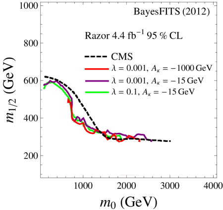
The 95% C.L. razor contour thus reproduced is shown in Fig. 1. The actual 95% C.L. line obtained by CMS is also shown as a dashed black line (we point out that the actual official line and the one obtained by CMS using the hadron box only are very close to each other). The relevant CNMSSM parameters were fixed as , , , and . The produced line is indicated in purple. One can see that the CMS limit is reproduced very well in the limits of and vice versa. A slight discrepancy in between those two extremes is basically irrelevant, as we shall see below. The dependence of the limit on and is negligible, since these parameters only affect the boundaries of the physically allowed region but do not cause a shift in the position of the contour. This is clear from Fig. 1, where we show a contour for (in green) and another for (in red), fixing the other parameters to the stated value in each case. The negligible dependence of the razor limit on , and sgn() has already been verified in many analyses; see e.g., [70, 71, 43]. Our choice of these parameters thus only ensures the maximum allowed physical region in the (, ) space, since the physicality aspect is later taken into account during the scan when the unphysical points are discarded.
3.3 Likelihood for the Higgs bosons
The measured mass of the Higgs-like boson has important consequences for global properties of the CNMSSM.
An absolute upper bound on the mass of a SM-like can be obtained in the limit (for which the singletlike scalar becomes very heavy) and is given by [72, 7]
| (6) |
where denotes loop corrections, and is the tree-level Higgs doublet vev. The second, NMSSM-induced term on the right-hand side of Eq. (6) can enhance the mass by a few beyond its MSSM value, if is large enough, , and . For larger values of , the second term on the right-hand side becomes suppressed, and the third, negative term becomes significant. Then, the value of the Higgs boson mass can only be enhanced by the loop corrections. As we shall see, when other constraints are taken into account, especially the ones coming from the LEP Higgs searches, -physics, the muon anomalous magnetic moment, , and DM relic density, the aforementioned conditions on and become hard to satisfy and drastically restrict the parameter space of the model.
As noted in the Introduction, in the NMSSM either of the two lightest
-even Higgses could serve the role of the SM-Higgs-like boson
observed at the LHC. There are thus three interesting possibilities
entailing such a discovery:333We assume that the third -even Higgs
is always heavier than the current experimental reach.
Case 1: ,
Case 2: ,
Case 3: .
3.3.1 Mass likelihood
In this paper we analyze all three cases mentioned above. We will henceforth refer to our selected 125.8 signal Higgs for either of the first two cases generically as . We impose a mass requirement on through a Gaussian likelihood which takes into account both the theoretical () and experimental () errors, following the procedure detailed in Ref. [43],
| (7) |
The theoretical error is due to residual differences between calculations using different approaches and schemes, and it is estimated in the literature to be of the order of 2–3 [73]. We assume . We use the CMS determination of the Higgs mass rather than the one by ATLAS, since it has been most recently updated, and also for consistency with our previous work [43].
3.3.2 Cross section likelihood
In order to be thoroughly consistent with the CMS measurement, we need to calculate for both Higgs bosons the reduced cross sections, defined in the literature as
| (8) |
for a given Higgs decay channel, .
Equation (8) can be approximated by
| (9) |
where the sum runs over the Higgs production channels ( for gluon-fusion, for vector boson-fusion and Higgs-strahlung off a boson, and for associated Higgs production with top and bottom quarks, respectively), and the ratios are obtained from the public tables provided by the LHC Higgs Cross Section Working Group [74, 75] for .
The reduced cross sections for the individual production channels are provided by the mass spectrum generator included in the NMSSMTools package, which we use for our analysis. Alternatively, they can be expressed in terms of the Higgs reduced couplings (the ratio of the couplings of the Higgs boson with a given mass to a pair of particles in the NMSSM, to the ones calculated in the SM) and the decay branching ratios , which are also provided by the mass spectrum generator,
| (10) | |||||
where the sum runs over the decay channels open to the SM Higgs boson.
We require and to comply with the measured rates, [1] and [4], respectively.444We only use the dominant decay channels where a excess has been observed. For the channel the “signal” likelihood is taken to be a Gaussian around the measured central value,
| (11) |
with being the experimental error. For the channel, since the experimental error is asymmetric, the signal likelihood is defined in terms of half-Gaussians for the positive error and negative error each, as done in the case of the likelihood above. is a very conservative estimate of the theoretical error based on [76], used for every channel .
In addition to constraining , there is another crucial aspect of cases 1 and 2, which is that the second of the two lightest -even Higgs bosons must have escaped detection at the LHC (or at LEP if very light), or be “hidden.” In the following we refer to it as . In other words, the production rate of should be less than what the experiments are currently sensitive to for all . As a result, should also be constrained by experimental data, so that all points where the rate of is large enough for it to have been observed are rejected in our analysis. For this purpose, we construct an “exclusion” likelihood. Following the procedure outlined in [62] for exclusion bounds we first define a step function,
| (12) |
where is the value of the signal strength modifier that is excluded at 95% C.L. by the LHC searches for a Higgs with a given mass , obtained from the latest exclusion plots published by the CMS Collaboration [77].555We used the latest exclusion limits provided based on 5.1/fb of data at and 12.2/fb of data at for the channel, on 4.9/fb at and 12.1/fb at for the channel and on 17/fb at for the channel. Limits for the channel have not been updated by CMS and are, therefore, still based on a combination of 5.1/fb at and 5.3/fb at of data. The LEP exclusion limits are taken into account by NMSSMTools beforehand.
Then, in order to include the theoretical error on the true values of the reduced cross section and the Higgs mass, is smeared out further by convolving it with Gaussian functions centered around their true theoretical values and , respectively, so that the exclusion likelihood now becomes
| (13) |
where the theoretical errors are taken to be and [76], respectively. The exclusion likelihood is calculated for , , and . Finally, in order for our exclusion criterion to be consistent with our criterion for signal observation at (with theory and experimental errors added in quadrature), we further impose the condition
| (14) |
For case 3, the likelihood in Eq. (7) is separately computed for both and . In this scenario, only the combined production rate for and needs to be equal to . Hence the observation likelihood is now defined as
| (15) |
The values and uncertainties of our Higgs constraints are given in Table 1.
4 Methodology and Results
The scanned ranges of the CNMSSM parameters along with the type of distribution of their prior are listed in Table 2. Also listed in the table are the input ranges of the nuisance parameters included in the scans. The sign of is fixed to or for a given scan.
The reason for choosing the given range of is twofold. First, we have checked that allowing lower values of hardly increases the number of points allowed by the physicality conditions. Second, allowing very small values of would have most likely driven the scan towards a purely CMSSM-like scenario, thus preventing us from scrutinizing any characteristic features of the CNMSSM, particularly for case 1.
| CNMSSM parameter | Description | Prior range | Prior distribution |
|---|---|---|---|
| Universal scalar mass | 100, 4000 | Log | |
| Universal gaugino mass | 100, 2000 | Log | |
| Universal trilinear coupling | , 7000 | Linear | |
| Ratio of Higgs vev’s | 1, 62 | Linear | |
| Higgs trilinear coupling | 0.001, 0.7 | Linear | |
| Nuisance | Description | Central value std. dev. | Prior distribution |
| Top quark pole mass | Gaussian | ||
| Bottom quark mass | Gaussian | ||
| Strong coupling | Gaussian |
The analysis was performed using the package BayesFITS which engages several external, publicly available tools: for sampling it uses MultiNest [78] with 4000 living points, evidence tolerance factor set to 0.5, and sampling efficiency equal to 0.8. Mass spectrum, along with , is computed with NMSSMTools v3.2.1 [66] and passed via SUSY Les Houches Accord format to SuperIso v3.3 [79] to calculate , , , and . DM observables, such as the relic density and direct detection cross sections, are calculated with MicrOMEGAs 2.4.5 [80].
Below we will present the results of our scans as one-dimensional (1D) or two-dimensional (2D) marginalized posterior pdf maps of parameters and observables. For example, in evaluating a posterior pdf for a given parameter, we marginalize over all of the model’s other parameters and the SM nuisance parameters, as described in detail in Refs. [43, 54].
Notice that when discussing the results of the global scan for case 1 it will become apparent that this case presents a remarkable CMSSM-like behavior. It would therefore be natural to try to compare those results with our recent CMSSM analysis [43]. In doing so, one needs to take into account the differences between the numerical codes and constraints adopted in both studies. We summarize them here.
1. In the present study we use NMSPEC (included in NMSSMTools) for calculating the supersymmetric spectrum, while in [43] we used SOFTSUSY. We have repeatedly cross-checked the spectra obtained in the MSSM limit of the NMSSM with the ones generated by SOFTSUSY, finding some differences, especially with respect to loop corrections giving the largest values of the lightest Higgs mass. In some regions of the parameter space the difference between the two generators can amount to a maximum of –1.666The best agreement between SOFTSUSY and NMSSMTools is obtained by setting the flag precision for the Higgs masses to zero which, therefore, was chosen as the default setting for our calculations. Given the experimental and theoretical uncertainties in the Higgs mass, such difference translates into units of , which is not significant for the purpose of the global scan.
2. In this paper we use the value of measured at LHCb [48], which has been incorporated in the likelihood as described in Sec. 3.1. The SM rate rescaled by the time-dependent asymmetries is now [64], which is a value more appropriate for comparison with the experimental rate than the unscaled, , one.
3. We have updated the nuisance parameters and following [51]; see Table 2. The upgrade in has significant implications for . The leading one-loop corrections to the Higgs mass squared are given by
| (16) |
where is the running top quark mass,777Note that the running top quark mass is related to the pole mass through the formula given in Eq. (10) of Ref. [81]. is the geometrical average of the physical stop masses, , and . Since it is now easier to generate Higgs masses in agreement with the experimental values. In particular, as we highlighted in [43], a Higgs mass compatible with the observed excess at 126 was rather difficult to achieve over the CMSSM parameter space. That tension has now become somewhat reduced, and we will show below that the correct Higgs mass can be obtained in the CMSSM limit of the CNMSSM.
4.1 Impact of the relic density
To set the ground for the presentation of our numerical results, we first comment on the role of the relic density of DM in selecting favored regions. The relic density is a strong constraint, since it is a positive measurement (in contrast to a limit) with a rather small experimental uncertainty (Table 1). On top of it, it is well known that in unified SUSY models with neutralino LSP the corresponding abundance is typically too large, or in other words, its annihilation in the early Universe is “generically” too inefficient, so that specific mechanisms for enhancing it are therefore needed. They, however, are only applicable in specific SUSY configurations. As a result, in most cases the regions of high probability in the global posterior will reflect one or more of the regions of parameter space where is close to the measured relic density of DM. The regions that are still allowed by direct SUSY searches are as follows:
1. The stau-coannihilation (SC) region [82]. As is known, in constrained SUSY models, like the C(N)MSSM, this is a narrow strip at a sharp angle to the axis. The values of and are also constrained, as only for not exceeding –3 and not too large does the mass of the stau become light enough to be comparable with the neutralino mass, but not so light as to make it the LSP. Values of that are excessively large, on the other hand, can suppress the annihilation cross section [83]. After other relevant constraints are included, the parameters of interest are, therefore, , , and, when the neutralino is close to 100% bino, . A similar effect can also be obtained for large with the stop replacing [84].
2. The -funnel (AF) region, where neutralinos annihilate through the resonance with the lightest pseudoscalar [85]. This mechanism can occur over broad ranges of the (, ) plane where the pseudoscalar mass is close to twice the neutralino LSP mass, and is enhanced by large () and positive .
3. The focus point/hyperbolic branch (FP/HB) region [86, 87], where the annihilation cross section can be enhanced by an increased higgsino component of the neutralino. For this to occur, (or in the NMSSM) must be of the order of a few hundred GeV, and cannot be too large, . In the (, ) plane the condition corresponds to the region where .
4.2 Impact of the Higgs mass
The measurement of the Higgs mass has added an important additional constraint on unified SUSY models. Below we will be discuss in turn the three cases listed earlier in Sec. 3.3.
Case 1.
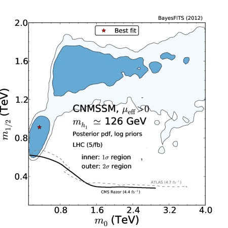
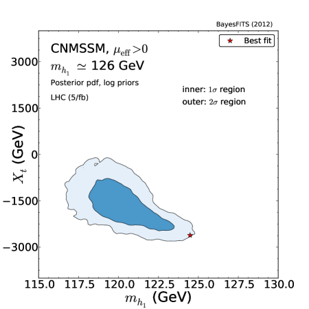
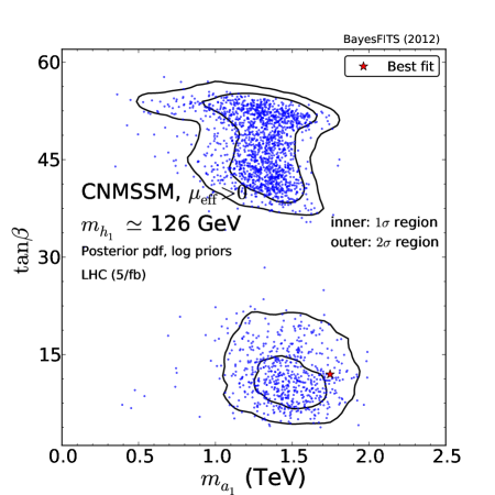
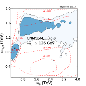
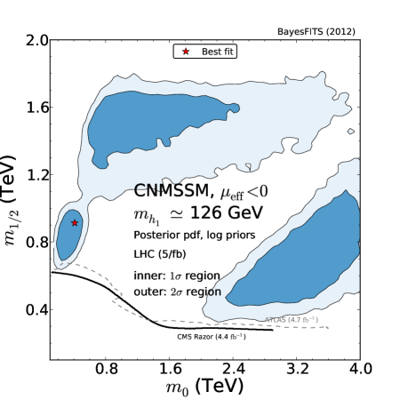
In Fig. 2LABEL:sub@fig:-a we show the marginalized posterior pdf in the (, ) plane of the CNMSSM for case 1, obtained by imposing simultaneously all the constraints shown in Table 1. In these and the following plots the Bayesian 68% () credible regions are indicated in dark blue and the 95% () credible regions in light blue. Notice that the regions of high probability are located above the CMS razor limit, which we implemented in the likelihoood as described in Sec. 3.2, and which is shown in the plots as a solid black line. In case 1 the role of the SM-like Higgs is played by the lightest -even scalar (almost purely -like), while (almost purely -like) and (almost purely singletlike) are usually much heavier and decoupled. This case is thus expected to present features very similar to the CMSSM.
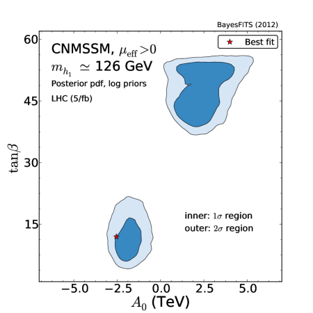
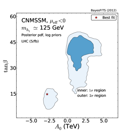
In Fig. 2LABEL:sub@fig:-a one can see two main 68% credibility regions: the SC region on the lower left side, and the AF region on the top part of the plot. As is also the case in the CMSSM, besides giving the correct relic abundance, the SC region shows also the better fit to the Higgs mass, . This is because, as we explained in Ref. [43], in the SC region can easily be negative without spoiling the relic abundance constraint. Large negative values of are necessary to drive the parameter to even larger negative values at the EW scale, thus making the stop mixing contribution to the loop corrections of the Higgs mass maximal. Note as well that the best-fit point is also located in the SC region.888We postpone further discussion of the best-fit points until Sec. 4.7. In Fig. 2LABEL:sub@fig:-b we show the marginalized posterior in the (, ) plane. The high probability “island” at negative and corresponds to the SC region.
In the CNMSSM the SC region appears to be more extended relative to the CMSSM [43], and somewhat larger Higgs masses also seem preferred, as we will show below. The increased relevance of the SC region is due to the fact that it is now much easier to obtain values of the Higgs mass closer to the correct one. This could be mistakenly thought to be a specific feature of the CNMSSM extended Higgs sector. We have checked that this is not the case: the Higgs mass is simply quite sensitive to the increased central value of the top mass, as we explained at the beginning of this section.
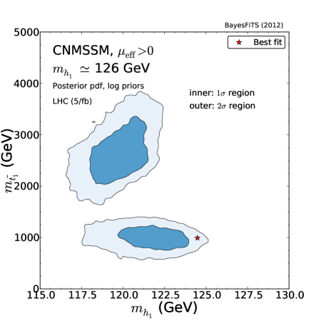
In Figs. 3LABEL:sub@fig:-a and 3LABEL:sub@fig:-b, we show how the constraints affect the main observables responsible for the loop corrections to the Higgs boson mass. In Fig. 3LABEL:sub@fig:-a, we show the posterior in the (, ) plane. Notice that the lightest stop does not have to be excessively heavy in the SC region, , since large stop mixing compensates for smaller . The correct Higgs mass is obtained since , as can be seen in Fig. 3LABEL:sub@fig:-b where we plot the posterior in the (, ) plane. On the other hand, one can see that in both figures the best-fit point lies outside of the 68% credibility regions of the marginalized 2D pdf, when the latter is projected to the plane of these observables. This is a feature not uncommon in Bayesian analyses where the credibility regions map the “volume” of scan points satisfying well enough a certain set of constraints, rather than representing isocontours of the likelihood function, as is the case in frequentist analyses. The fact that the best-fit point is situated outside of the region of highest posterior probability for the considered observables simply tells us that, while for this point all the constraints are very well satisfied, it is also not very likely to obtain a similarly good value of the observable for similar choices of the input parameters. Particularly, in the case of Figs. 3LABEL:sub@fig:-a and 3LABEL:sub@fig:-b, the majority of the points that satisfy all the constraints in the SC region present a Higgs mass in the range 120–123, while for the other regions it is even less.
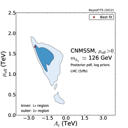
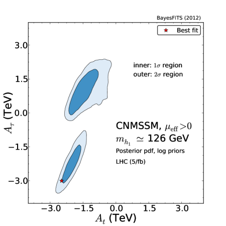
Figure 2LABEL:sub@fig:-a also shows that the Higgs mass constraint favors the part of the AF region situated at for a broad range of values. Besides, in Fig. 2LABEL:sub@fig:-b one can see that in the (, ) plane the AF region spans a large range of positive values and is constrained to . In this region one-loop corrections to the Higgs mass are driven up by a large stop mass (–4, as shown in Fig. 3LABEL:sub@fig:-a) rather than large stop mixing which, given the preferred values of , is minimal (see Fig. 3LABEL:sub@fig:-b). Large values of push the Higgs mass close to the experimentally observed value, but not enough to reach it (for even larger , becomes too heavy and resonant annihilation of neutralinos is not efficient). This can be interpreted as a sign of some tension between the relic abundance and Higgs mass constraints in the AF region, which was investigated for the CMSSM in our previous paper [43]. The tension persists in the CNMSSM.
Only a limited fraction of the FP/HB region (which appears as a narrow 95%-credibility “tail” at ) survives, as was the case for the CMSSM, despite the fact that the relic density is well satisfied over there. As we pointed out in [43], some tension with the 126 Higgs boson mass arises not only in the AF but also in the FP/HB region where is smaller than anywhere else. In fact, small values of can be obtained only for relatively small values of , as can be seen in Fig. 4LABEL:sub@fig:-a, where we show the posterior in the weak scale parameters and (notice that over all parameter space). For the chosen range of , in the FP/HB region cannot be very large either, so that the correct Higgs mass cannot be reached. The region of high posterior thus moves up towards larger , where the neutralino has still a non-negligible higgsino component, but is large enough to give the correct Higgs mass.
It is worth pointing out that is not realized in the CNMSSM. This is because the lightest pseudoscalar becomes nonphysical for such values. The mass of is, for moderate and large values of , well approximated by [88]. and are unified to at the GUT scale, and barely runs, since the one-loop contribution to its -function is negligible. As a consequence, in the CNMSSM and have always opposite signs and there are no points in the scan with or .
We present in Fig. 4LABEL:sub@fig:-b the marginalized posterior pdf in the (, ) plane. The parameters show a clear linear correlation, which in the SC region (bottom left corner) results in large negative values for both observables, due to the fact that the correct Higgs boson mass requires large stop mixing, as discussed above.

Figure 5 shows the 2D posterior in the (, ) plane. One can notice the known correlation between and [44], as in general cannot exceed a given value of by too much without causing a Landau pole in RGE running (see e.g. [88] for details) and, on the other hand, cannot exceed a given value of by too much because the increased mixing between the doublet and singlet states lowers much below the observed value, where the likelihood becomes negligible, and eventually below the LEP bounds [52]. In the SC region is positive since is negative, while in the AF and FP/HB regions these parameters switch signs. Hence, the upper branch shown in Fig. 5 corresponds to the SC region, and the lower one to both the AF and the FP/HB regions. Notice also that the upper branch is narrower than the lower one, due to the fact that SC occurs for limited ranges of the (), (large and negative) and (–2) parameters. As a consequence, the condition for electroweak symmetry breaking requires to be very close to in the SC region.
At 95% credibility, the branches stretching along show an absolute upper bound in , which changes slightly for regions of parameter space characterized by different mechanisms to reduce the relic abundance. Specifically one can see that, on the one hand, for the upper branch. Again, for the ranges of parameters required by SC, a larger lowers below the scale preferred by the likelihood function because of the increased singlet-doublet mixing [7]. On the other hand, in the AF region (right-hand part of the lower branch) cannot exceed 0.12 by too much as this would increase , pushing it off the resonance with the lightest neutralino. In the FP region (left-hand part of the lower branch) the bound is on negative , and is due to the chosen ranges for () and the fact that tends to be small there, as shown in Fig. 4LABEL:sub@fig:-a. Simply, when is significantly below , it becomes difficult to obtain electroweak symmetry breaking.
We want to reemphasize that, when the global constraints are considered, case 1 presents a very CMSSM-like character. The parameter is small, and its effect on is insignificant, given that over all of the regions of high posterior probability, as shown in Fig. 2LABEL:sub@fig:-b. In the SC region the lightest Higgs mass can assume values close to 126 more easily than what was observed in our work on the CMSSM, but the reason lies in the updated value of the top mass used for the present analysis.
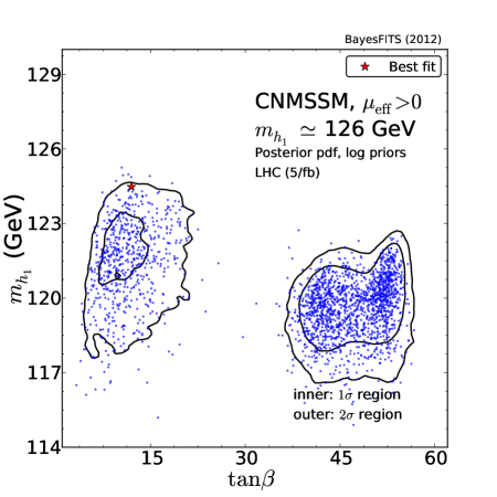
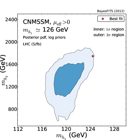
In Fig. 6LABEL:sub@fig:-a we show the marginalized posterior in the (, ) plane and in Fig. 6LABEL:sub@fig:-b the posterior in the (, ) plane. We also overlap a distribution of samples uniformly selected from our nested sampling chain. Notice that the density of samples reflects their relative posterior probability. One can see in Fig. 6LABEL:sub@fig:-a that, in the SC region (left island) the tension between the correct Higgs mass and the other constraints is much ameliorated. Figure 6LABEL:sub@fig:-b shows confirmation of the CMSSM-like nature of this case, as the pattern of high posterior mirrors the one found in Ref. [43].
Case 2.
The NMSSM allows more freedom in the Higgs sector than the MSSM, due to the extended number of parameters. Even in its partially constrained version, there is a possibility of obtaining a light , which we found to be a mixture of and fields. A non-negligible singlet component creates the difference in the Higgs sector between this scenario and case 1. In the rest of this section we analyze the consistency of an signal with the observed excess at the LHC.

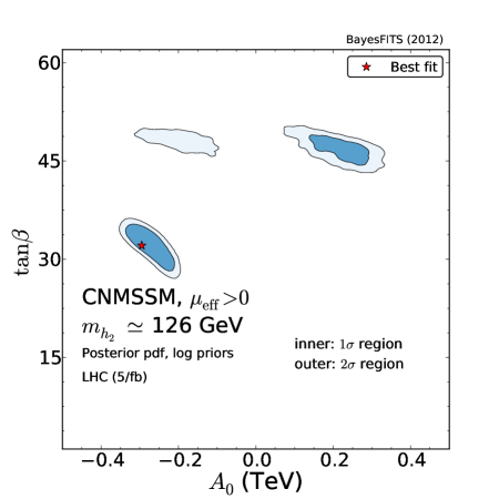
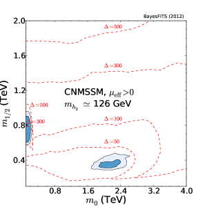
In Fig. 7LABEL:sub@fig:-a we show the posterior pdf in the (, ) plane for case 2. The favored parameter space is now drastically reduced with respect to case 1. Only the SC region, where the best-fit point is located, and the FP/HB region survive the requirement of having .
In Fig. 7LABEL:sub@fig:-b we show the posterior pdf in the (, ) plane. In both regions the range preferred for does not extend much from zero, .999Note that a gap around in Fig. 7LABEL:sub@fig:-b comes from the physicality condition for , as discussed above. The reason is that is now limited to values less than 400 by our requirement on the mass of . Specifically, under the assumption of a moderate-to-large and as long as the parameters , , and do not exceed the EW scale by too much, a good approximation to the masses of the two lightest -even Higgs bosons at the tree level was found in [88]:
| (17) |
In Eq. (17), the second term under the square root is suppressed with respect to the EW scale because is small, as we shall see below. One can see that in the regime where , the mass of is of order and scales as . Thus, the physicality condition translates into the approximate relation . On the other hand, in the regions where , and . Values of much greater than 126 are disfavored by the likelihood function, so that presents an upper bound, which translates into an upper bound on .
Since in most of the parameter space is very large, and and are correlated, the scan also shows upper bounds for and , in a fashion very similar to what is shown in Fig. 5 for case 1. For case 2, in the SC region is very small, , while in the FP/HB region it can assume slightly larger values, . Obviously, the upper bound on does not depend on any particular position in the parameter space, but the bound on (or ) does, and is affected particularly by . In the SC region while in the FP/HB region .
Given the strong constraint on placed by the mass of , the only way of obtaining the relic density though coannihilation with the lightest stau is if the lightest neutralino is a nearly pure singlino and very light. This is exactly what is observed in the SC region and, as a consequence, in that region and are bounded to be much smaller than in case 1 (the neutralino mass matrix with the convention used in this paper can be found, e.g., in [44]), can only be negative, and assumes larger values (, favored also by other constraints, e.g. ) than in the same region of case 1, or of the CMSSM. For smaller values of , or a positive , the neutralino would be mostly bino and the lightest stau would be the LSP.
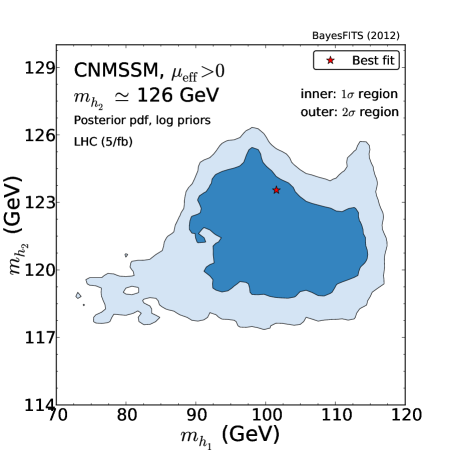
In Figs. 8LABEL:sub@fig:-a and 8LABEL:sub@fig:-b we show the 2D posterior in the (, ) plane for case 1 and case 2, respectively. One can see that in case 1 , while in case 2 the 68% credibility region shows a preference for .
Since in case 2 , assumes values quite small in the favored regions, . While it might appear that such a case is excluded by the recent searches at the LHC [89], we point out that the limit does not apply to this case, as the relevant couplings for and are suppressed by the pseudoscalar mixing angle , i.e., when [90]. We have checked that is very close to zero over the regions of interest.
Case 3.
Case 3 (two degenerate light Higgs bosons) is in fact a subset of case 2 when it comes to the preferred parameter space, which is uniquely determined by the requirement of as was explained above. The 2D posterior pdf’s for the input parameters are in this case almost indistinguishable from the ones showed in Figs. 7LABEL:sub@fig:-a and 7LABEL:sub@fig:-b, and the best-fit point is again situated in the SC region. We therefore refrain from showing them explicitly. However, this case presents also some characteristic features:
is a mixture of and , with a predominance of the latter, while is mainly singletlike, with a small fraction of .
Both and are now much more limited and very close to zero. The reason for this is simple: in order to have the two lightest -even Higgs bosons almost degenerated in mass, one needs to minimize the difference from Eq. (17). This yields negligible values for the parameter and, consequently, also for . Clearly, as a consequence, the singlino nature of the LSP in the SC region is a feature confirmed for case 3.
4.3 Impact of the cross section rates
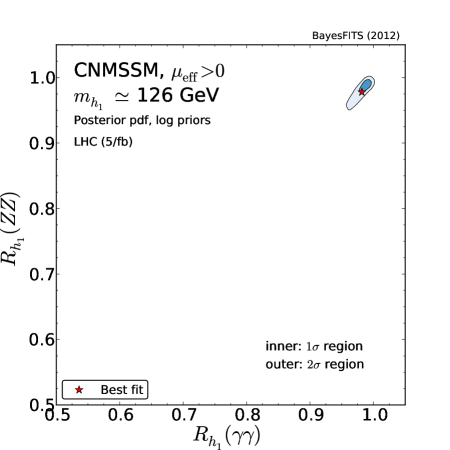

In Fig. 9LABEL:sub@fig:Rs_a we show the 2D posterior pdf in the (, ) plane for case 1. As one can see, the Higgs boson in this case is SM-like. Actually, it is known [29] that the enhancement of the signal strength in the decay channel observed by both CMS and ATLAS cannot be obtained for the values of that are favored by the global scan. As a consequence, cannot be fitted perfectly in the CNMSSM. This discrepancy effectively adds two units of homogeneously over the preferred parameter space, but it does not alter the posterior distribution. For the same reason cannot be perfectly fitted either, though its contribution to the total is smaller than 0.5 units of , making this observable equally ineffective in constraining the posterior.
In Fig. 9LABEL:sub@fig:Rs_b we present the posterior distribution for case 2. Once again, can hardly become larger than 1 over the preferred parameter space. The 95% credible region lies far from the central value of the observed enhancement and, in fact, even covers values lower than in case 1. presents similar behavior, although the suppression of the reduced cross section is highly welcome for this observable, as it places the calculated value closer to the rate observed at CMS. Smaller than 1 signal rates indicate less of a SM-like character for , which is caused by the suppression of the SM couplings induced by its increased singlet component.
The posterior distributions presented in Figs. 9LABEL:sub@fig:Rs_a and 9LABEL:sub@fig:Rs_b indicate that, in both case 1 and case 2 it is in general extremely difficult to obtain the signal enhancement in the channel. The scan naturally tends to stay in the regions of parameter space favored by all constraints. It is therefore no surprise that among the points scanned for case 1 only two presented a rate in the range 1.2–2, thanks to the reduced coupling of the signal Higgs boson to the bottom quarks. Such points present contributions to the relic density of order several 10s, and the contribution to is of order 100. In case 2 we found a dozen such points, for which the contribution to the relic density is even worse.
In case 3 one could expect to obtain an enhancement of by adding the individual rates for both almost degenerate light scalars. However, the posterior pdf in the (, ) plane is remarkably similar to the one shown in Fig. 9LABEL:sub@fig:Rs_a, due to the large singlet component of , and we refrain from showing it again over here. In fact, in case 3 we were not able to find a single point with the enhanced rate. Since case 3 is a subset of case 2 in terms of the favored parameter space, and the rates in the and channel do not show interesting features, we will not consider it separately from the other cases any further.
4.4 Prospects for DM direct detection and
In this subsection we will discuss the impact of limits from direct DM searches on the preferred parameter space of the CNMSSM. This kind of experiments are complementary to direct LHC SUSY searches, as they are capable of testing neutralino mass ranges beyond the current and future reach of the LHC, and therefore could add new pieces of information to the global picture.
At present the most stringent limit on the spin-independent cross section comes from XENON100 [91]. In supersymmetric models it can then be plotted as a function of the neutralino mass in the form of an exclusion limit in the (, ) plane.
We want to point out that the theory uncertainties are very large (up to a factor of 10) and strongly affect the impact of the experimental limit on the parameter space [54]. It was shown that, when smearing out the XENON100 limit with a theoretical uncertainty of order 10 times the given value of , the effect on the posterior is negligible for regions of the parameters that appear up to 1 order of magnitude above the experimental line. Moreover, the main source of error (the so-called term) arises from different, and in fact incompatible, results following from different calculations based on different assumptions and methodologies. Therefore, in this study we decided not to include the upper bound on from XENON100 in the likelihood function, but below we will discuss its possible effects on the properties of the model.
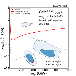
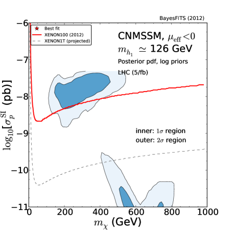
In Fig. 10LABEL:sub@fig:h1sigsip-a, we present the posterior pdf in the (, ) plane for the case 1. The solid red line shows the most recent 90% C.L. upper exclusion limit by the XENON100 Collaboration. One can see that the two high posterior probability regions (from SC on the left and AF on the right) are located well below it. A small 95% credible region (corresponding to the FP/HB region with the lightest neutralino being a mixture of bino and higgsino) would probably be excluded by adding the XENON100 limit to the likelihood, even taking into account significant theoretical uncertainties. One can also notice that XENON1T, a future ton-size DM detector (projected sensitivity represented as the dashed gray line), will be in a position to test the 68% credible regions.
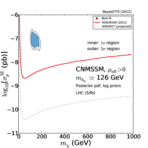
The conflict with the XENON100 limit in case 2 (and case 3, which presents similar features) is even stronger. In Fig. 10LABEL:sub@fig:h1sigsip-b we show the posterior in the (, ) plane. The high probability region above the experimental line presents the features of the FP/HB region: , and the lightest neutralino is a mixture of bino and higgsino. As a consequence, the spin-independent neutralino-proton cross section is larger and in this case already in strong tension with the XENON100 bound.
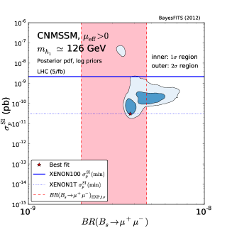

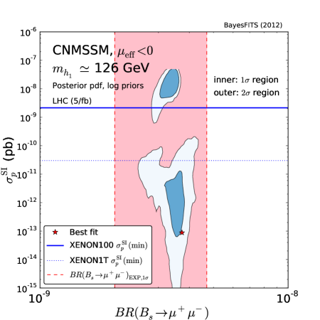
Notice that the SC region is not shown in Fig. 10LABEL:sub@fig:h1sigsip-b since the neutralino is a nearly pure singlino there, so that is several orders of magnitude below the XENON100 bound (and below the range shown in the figure). However, we would like to point out that in case 2 (and case 3) strong constraints on the full parameter space can be placed as a result of the interplay between the limits provided by two completely different experiments –that test different observables by means of different experimental techniques –namely LHCb and XENON100. This is illustrated in Figs. 11LABEL:sub@fig:-a and 11LABEL:sub@fig:-b, where we show the posterior pdf in the plane for case 1 and case 2, respectively. The solid blue horizontal line shows the minimum 90% C.L. upper bound on by XENON100 (obtained at ), and the dotted blue horizontal line the corresponding projected sensitivity for XENON1T. The pink vertical band encompasses the experimental uncertainty on the recent LHCb measurement of [48]. Figure 11LABEL:sub@fig:-b shows that, for cases 2 and 3, in the SC region is strongly enhanced, due to the large values assumed by there, and it could be excluded by the next updated results from LHCb.
4.5 Fine-tuning
In this subsection we will address the issue of fine-tuning. Note that we will not delve into it, nor will we discuss which values of fine-tuning are acceptable or not from the point of view of naturalness. Our aim here is to simply present an estimate of fine-tuning (provided as an output by NMSSMTools v3.2.1) for the preferred parameter space of the model, leaving aside the discussion of the viability of the model itself, which would be a matter of personal prejudices.
The mass of the boson (which determines the EW symmetry breaking scale) can be expressed in terms of the supersymmetric parameters through the minimization condition of the Higgs potential,
| (18) |
The fine-tuning problem of the MSSM [92] amounts to the fact that the parameters , and need to be simultaneously tuned to a high precision to reproduce the correct value of . In the NMSSM is replaced by .
In the framework of the unified theory, at the GUT scale . They are then evolved down to the EW scale by means of the RGEs. Therefore, the right-hand side of Eq. (18) depends on the parameters of the model at the GUT scale.
The measure of fine-tuning associated with the parameter of the model is defined as [93, 92]
| (19) |
In the CNMSSM, . We do not present the fine-tuning measure due to the top quark Yukawa coupling, following the approach adopted in [87], and quantifying the fine-tuning associated only with the supersymmetric parameters. We define the fine-tuning measure for a given model point as the maximal contribution to fine-tuning among all the model’s parameters for that point,
| (20) |
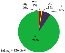
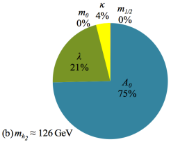
In Figs. 12LABEL:sub@fig:-a and 12LABEL:sub@fig:-b we present the isocontours of the fine-tuning measure in the (, ) plane for cases 1 and 2, respectively. The isocontours reflect the value of for the vast majority of the points included. They are superimposed on the 2D posterior distributions. Case 1 presents very CMSSM-like behaviour, where smaller fine-tuning can be achieved only in the FP/HB region due to the relatively low values of . Note that for the same reason is larger in the SC region which is characterized by larger . On the other hand, case 2 is less fine-tuned ( in a vast region of the parameter space preferred at ), which is a reflection of the fact that the parameter space is already highly constrained by the requirement of . In Figs. 13LABEL:sub@fig:-a and 13LABEL:sub@fig:-b we show for what percentage of the total number of allowed points each of the ’s yields maximal fine-tuning. For example, gives maximal fine-tuning for 94% of the points in case 1, while is the main contributor for the vast majority of the points in case 2.
4.6 Relaxing and the case of negative
In our recent study of the CMSSM [43] we considered the effect of relaxing the constraint. The reason was based on the observation that the poor fit of the CMSSM was the result of basically that single constraint, which simply could not be reproduced after including especially direct superpartner mass limits from the LHC. This appears to be a general feature of all SUSY models where slepton and squark masses are assumed to be comparable, including simple unified models like the CMSSM or CNMSSM. We simply state it as a conclusion reached by many studies. While we do not feel to be in a position to comment on the reliability of theoretical calculations of the SM which are strongly affected by nonperturbative effects related to low-energy strong interactions, especially the hadronic light-by-light contribution (for more details see, e.g., the Introduction of [43] and references therein), we believe that it thus makes sense to consider global scans where the constraint is removed. We showed in [43] that for the CMSSM the better fit was obtained with thanks to the constraints from -physics, which present a much better for this choice of parameters.
Relaxing the constraint in the CNMSSM while keeping positive has no apparent impact on the posterior distributions both for the parameters of the model as for the measured observables. Such behavior was to be expected for case 1, as it was already observed for the CMSSM in [43]. We checked that this is true also for case 2 and case 3, where relaxing the constraint while keeping positive has little effect. Specifically, it reduces the statistical relevance of the SC region and slightly increases the size of the posterior in the FP/HB region where, as we discussed in Sec. 4.4, it is disfavored by the XENON100 bound.
We also confirm that, for case 1, the better overall fit is obtained with for basically the same reasons as in the CMSSM. In Fig. 14LABEL:sub@fig:-a we show the 2D posterior pdf in the (, ) plane for case 1, where we ignored the constraint from and set . Differently from the CMSSM, where one could observe a clear predominance of the AF region, in the CNMSSM the SC, AF and FP/HB regions of parameter space now seem to be equally probable. This is not likely to be an intrinsic difference between the CMSSM and the CNMSSM; it is more probably due to the fact that the constraints are implemented with different numerical tools in the two models, as explained exhaustively at the beginning of Sec. 4. We note here that the global likelihood becomes flat over the regions of parameter space preferred by the relic density, and very little information can be extracted from the posterior.
In Fig. 14LABEL:sub@fig:-b we show the same posterior pdf in the (, ) plane for case 1. As was the case for the CMSSM, one can see that the distribution of tends to favor slightly smaller values than in the positive case, particularly in the AF region.
In Fig. 15LABEL:sub@fig:-a we show the 2D posterior pdf in the (, ) plane for case 1. Since the posterior in the FP/HB region is much more extended with respect to the positive case, a large region of parameter space lies above the XENON100 bound, and has the potential of being tested with modest improvements in sensitivity. On the other hand, as was the case for the CMSSM, the AF region ( and ) is not likely to be further constrained by the new spin-independent cross section measurements planned for the next years, including XENON1T.
We shall analyze the contributions from the individual constraints in the next subsection. Here we only repeat that, when the constraint is relaxed, the better can be obtained for thanks to the improved fit to and . To illustrate this feature we show in Fig. 15LABEL:sub@fig:-b the 2D posterior pdf in the (, ) plane for case 1. When , a cancellation between the pseudoscalar and axial vector form factors [94] takes place, with the result of improving the fit to over all of the parameter space, and particularly in the AF region, where the calculated values are pushed below the SM value.
For case 2 and case 3 it was not possible to perform the analysis of the effects of , as the simultaneous interplay of different constraints strongly disfavors the entire parameter space of the model and no region of good fit appears. This can be understood by remembering that decisively favors small values of ( in the CNMSSM). On the other hand, physicality requires , which for means [7], or . Both constraints cannot be simultaneously satisfied for (, and negative) so that the scan tends to prefer small positive values of . This generates a conflict with the relic density constraint: in the SC region is required for singlino LSP, whereas in the FP/HB region, when and the higgsino component of the neutralino is reduced and the relic density becomes too large.
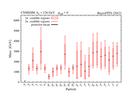
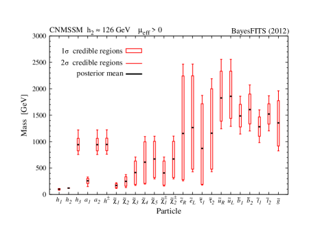
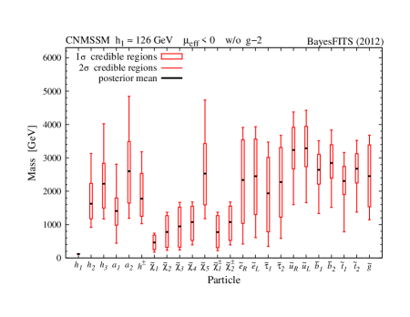
4.7 Mass spectrum and the best-fit points
 |
In Figs. 16LABEL:sub@fig:-a and 16LABEL:sub@fig:-b, we show the 1D marginalized posterior pdf’s for the SUSY mass spectrum in case 1 and case 2, respectively. The narrow lines indicate the 95% credibility regions, and the thick bars the 68% credibility regions.
Figure 16LABEL:sub@fig:-a shows the CMSSM-like character of case 1, since , and are all heavy and effectively decoupled from the low scale spectrum. For case 2, Fig. 16LABEL:sub@fig:-b shows that requiring forces the particles of the Higgs sector to be quite light, while the sfermions remain heavy, although they tend to be lighter than in case 1, since is lighter and it requires smaller loop corrections. The latter affect the scale of the stop and, through the assumption of unification, the other sfermions.
In Fig. 16LABEL:sub@fig:-c we show the mass spectrum for case 1 where we neglect and set . Again we confirm the CMSSM-like nature.
In Fig. 17 we show the individual contributions of the applied constraints to the best-fit point, for the cases considered in this study. As could be expected, in case 1 the main contribution comes from , once more confirming the CMSSM-like character of this scenario. In case 2 the contribution from is comparable to the one from , due to the singlino character of the neutralino which favors higher , as explained in Sec. 4.4. When , relaxing the constraint does not change significantly the contributions to due to the other constraints. This shows that the due to is fairly homogeneous throughout the parameter space not yet excluded by direct LHC SUSY searches. However, for negative the total improves by around 1–2 units, thanks to the improved fit to , for which the contribution from the chargino-stop loop changes sign and tends to enhance the branching ratio, towards the experimental value [95]. As a consequence, the overall fit to the experimental measurement improves.
One can finally notice that the contributions to due to are sizeable in all three cases, as was explained in Sec. 4.3.
In Table 3 we show the parameters of the best-fit points obtained in our scans.
| With | ||||||||
| Case 1, | 340.9 | 911.9 | 12.0 | 0.017 | 124.5 | 427 | 17.91 | |
| Case 2, | 102.8 | 803.6 | 32.1 | 0.006 | 123.5 | 396 | 18.45 | |
| Case 3, | 124.7 | 958.8 | 33.7 | 0.001 | 120.3, 126.2 | 480 | 20.08 | |
| No | ||||||||
| Case 1, | 410.2 | 913.3 | 14.8 | 0.017 | 123.9 | 455 | 6.40 | |
5 Summary and conclusions
In this paper we have presented the first global analysis of the CNMSSM which included the measurement of the mass and decay cross sections of the Higgs-like resonance observed at the LHC, the first evidence of nonzero at LHCb, SUSY mass limits from direct searches, as well as the updated value of the top mass. We discussed in detail the possibility of either one of the lightest -even Higgs bosons of the model playing the role of the SM-like Higgs (case 1 and case 2 in the text) and that of the observed excess being due to a combination of two of them, both lying within the range –129, after inclusion of a 3 theoretical error on the Higgs mass calculation (case 3 in the text).
In contrast to the case with , explored for example in [96], we found that with our choice of parameters the CNMSSM allows for a SM-like as heavy as 125, especially in the stau-coannihilation region where the scan obtains a good compromise between the relic density and the mass constraint, owing to large negative values. The calculated value of is larger than what was previously found for the CMSSM [43] thanks to the increased value of the top pole mass. The overall fit is somewhat spoiled by the requirement of having consistent with the value reported by the CMS Collaboration, since it is virtually impossible, given our parameter choice and ranges, to obtain an enhancement in the cross section rate in case 1. A similar conclusion can be drawn for case 2 where, in turn, is required to have a mass around 126, which can also be achieved but at the cost of a poor fit to other observables. Case 3, with almost degenerate and , was found not to be as interesting as anticipated, since the combined almost never exceeds 1, besides the fact that the high credibility posterior regions mimic those of case 2.
As mentioned in Sec. 2, we have adopted in this paper the choice at the GUT scale. We checked with a few preliminary scans that this choice does not affect the shape and position of the posterior pdf’s in case 1. This make sense since, as we explained in Sec. 4, to satisfy all the constraints the model tends to its CMSSM limit, and the singlet field effectively decouples from the theory. Similarly, relaxing the unification condition on would have little impact on the (, ) 2D posterior in case 2 and case 3. In both cases the requirement of a very light constrains and substantially through and the stop mixing parameter, independently of the value of at the GUT scale. As a consequence, the relic density can only be satisfied in the regions of the (, ) plane shown in Fig. 7LABEL:sub@fig:-a. Some differences, on the other hand, can be expected in the distribution of in case 2 and case 3. Particularly, in the stau-coannihilation region, where the LSP is singlinolike, the region of high probability is likely to extend to values of lower than the ones favored in this study. Consequently, the impact of the constraint is likely to be reduced.
On the other hand, even by disunifying , we would not expect changes relative to our analysis of the di-boson Higgs decay rates. In a recent paper [10] it was shown that a enhancement consistent with the observation is easily obtained in case 2. But we remind the reader that the study in question analyzed a model substantially less constrained than the one explored in here. In particular we have checked that, when allowing and to be free at the SUSY scale (as was done in [10]), the size of the favored parameter space in case 2 can increase significantly.
Finally, in this paper we also provided estimates of fine-tuning due to the various input parameters of the model in the form of isocontours in the (, ) plane for cases 1 and 2. We noted that the maximum fine-tuning for most of the parameter space comes from two different sources in the two cases.
We assessed the effects of abandoning the constraint since it cannot be reproduced in the CNMSSM, and more generally SUSY models with slepton-squark unification. In this case the overall fit actually improves considerably in case 1 for , due to a better agreement of the model’s predictions for -physics observables with experimental data, similarly to the CMSSM. Case 2 and case 3, on the other hand, are strongly disfavored for by the simultaneous impact of several constraints.
ACKNOWLEDGMENTS
S.M. would like to thank Cyril Hugonie for useful e-mail exchange regarding model implementation in NMSSMTools. L.R. thanks Gino Isidori and Matteo Palutan for helpful comments about .
This work has been funded in part by the Welcome Programme of the Foundation for Polish Science. K.K. is supported by the EU and MSHE Grant No. POIG.02.03.00-00-013/09. L.R. is also supported in part by the Polish National Science Centre Grant No. N202 167440, an STFC consortium grant of Lancaster, Manchester and Sheffield Universities and by the EC 6th Framework Programme MRTN-CT-2006-035505. The use of the CIS computer cluster at NCBJ is gratefully acknowledged.
References
- [1] CMS Collaboration, S. Chatrchyan et al., “Observation of a new boson at a mass of 125 GeV with the CMS experiment at the LHC,” Phys.Lett. B716 (2012) 30–61, arXiv:1207.7235 [hep-ex].
- [2] ATLAS Collaboration, G. Aad et al., “Observation of a new particle in the search for the Standard Model Higgs boson with the ATLAS detector at the LHC,” Phys.Lett. B716 (2012) 1–29, arXiv:1207.7214 [hep-ex].
- [3] “Combination of standard model higgs boson searches and measurements of the properties of the new boson with a mass near 125 gev,” Tech. Rep. CMS-PAS-HIG-12-045, CERN, Geneva, 2012
- [4] “Updated results on the new boson discovered in the search for the standard model higgs boson in the zz to 4 leptons channel in pp collisions at sqrt(s)=7 and 8 tev,” Tech. Rep. CMS-PAS-HIG-12-041, CERN, Geneva, 2012
- [5] “Updated atlas results on the signal strength of the higgs-like boson for decays into ww and heavy fermion final states,” Tech. Rep. ATLAS-CONF-2012-162, CERN, Geneva, Nov, 2012
- [6] J. E. Kim and H. P. Nilles, “The mu Problem and the Strong CP Problem,” Phys. Lett. B 138 (1984) 150.
- [7] U. Ellwanger, C. Hugonie, and A. M. Teixeira, “The Next-to-Minimal Supersymmetric Standard Model,” Phys.Rept. 496 (2010) 1–77, arXiv:0910.1785 [hep-ph].
- [8] M. Maniatis, “The Next-to-Minimal Supersymmetric extension of the Standard Model reviewed,” Int.J.Mod.Phys. A25 (2010) 3505–3602, arXiv:0906.0777 [hep-ph].
- [9] U. Ellwanger, “A Higgs boson near 125 GeV with enhanced di-photon signal in the NMSSM,” JHEP 1203 (2012) 044, arXiv:1112.3548 [hep-ph].
- [10] U. Ellwanger and C. Hugonie, “Higgs bosons near 125 GeV in the NMSSM with constraints at the GUT scale,” Adv.High Energy Phys. 2012 (2012) 625389, arXiv:1203.5048 [hep-ph].
- [11] S. King, M. Muhlleitner, and R. Nevzorov, “NMSSM Higgs Benchmarks Near 125 GeV,” Nucl.Phys. B860 (2012) 207–244, arXiv:1201.2671 [hep-ph].
- [12] J. Cao et al., “A SM-like Higgs near 125 GeV in low energy SUSY: a comparative study for MSSM and NMSSM,” JHEP 1203 (2012) 086, arXiv:1202.5821 [hep-ph].
- [13] D. A. Vasquez, G. Belanger, C. Boehm, J. Da Silva, P. Richardson, et al., “The 125 GeV Higgs in the NMSSM in light of LHC results and astrophysics constraints,” Phys.Rev. D86 (2012) 035023, arXiv:1203.3446 [hep-ph].
- [14] J. Rathsman and T. Rossler, “Closing the Window on Light Charged Higgs Bosons in the NMSSM,” Adv.High Energy Phys. 2012 (2012) 853706, arXiv:1206.1470 [hep-ph].
- [15] D. Das, U. Ellwanger, and P. Mitropoulos, “A 130 GeV photon line from dark matter annihilation in the NMSSM,” JCAP 1208 (2012) 003, arXiv:1206.2639 [hep-ph].
- [16] J. F. Gunion, Y. Jiang, and S. Kraml, “Could two NMSSM Higgs bosons be present near 125 GeV?,” Phys.Rev. D86 (2012) 071702, arXiv:1207.1545 [hep-ph].
- [17] J. F. Gunion, Y. Jiang, and S. Kraml, “Diagnosing Degenerate Higgs Bosons at 125 GeV,” Phys.Rev.Lett. 110 (2013) 051801, arXiv:1208.1817 [hep-ph].
- [18] R. Benbrik, M. Gomez Bock, S. Heinemeyer, O. Stal, G. Weiglein, et al., “Confronting the MSSM and the NMSSM with the Discovery of a Signal in the two Photon Channel at the LHC,” Eur.Phys.J. C72 (2012) 2171, arXiv:1207.1096 [hep-ph].
- [19] K. J. Bae, K. Choi, E. J. Chun, S. H. Im, C. B. Park, et al., “Peccei-Quinn NMSSM in the light of 125 GeV Higgs,” JHEP 1211 (2012) 118, arXiv:1208.2555 [hep-ph].
- [20] Z. Kang, T. Li, J. Li, and Y. Liu, “A Rediatively Light Stop Saves the Best Global Fit for Higgs Boson Mass and Decays,” arXiv:1208.2673 [hep-ph].
- [21] T. Cheng, J. Li, T. Li, X. Wan, Y. K. Wang, et al., “Toward the Natural and Realistic NMSSM with and without -Parity,” arXiv:1207.6392 [hep-ph].
- [22] M. Perelstein and B. Shakya, “XENON100 Implications for Naturalness in the MSSM, NMSSM and lambda-SUSY,” arXiv:1208.0833 [hep-ph].
- [23] G. Belanger, U. Ellwanger, J. Gunion, Y. Jiang, and S. Kraml, “Two Higgs Bosons at the Tevatron and the LHC?,” arXiv:1208.4952 [hep-ph].
- [24] J. Cao, Z. Heng, J. M. Yang, and J. Zhu, “Status of low energy SUSY models confronted with the LHC 125 GeV Higgs data,” JHEP 1210 (2012) 079, arXiv:1207.3698 [hep-ph].
- [25] G. Chalons and F. Domingo, “Analysis of the Higgs potentials for two doublets and a singlet,” Phys.Rev. D86 (2012) 115024, arXiv:1209.6235 [hep-ph].
- [26] G. Belanger, U. Ellwanger, J. F. Gunion, Y. Jiang, S. Kraml, et al., “Higgs Bosons at 98 and 125 GeV at LEP and the LHC,” JHEP 1301 (2013) 069, arXiv:1210.1976 [hep-ph].
- [27] I. Gogoladze, B. He, and Q. Shafi, “Inverse Seesaw in NMSSM and 126 GeV Higgs Boson,” Phys.Lett. B718 (2013) 1008–1013, arXiv:1209.5984 [hep-ph].
- [28] D. E. Lopez-Fogliani, “Light Higgs and neutralino dark matter in the NMSSM,” J.Phys.Conf.Ser. 384 (2012) 012014.
- [29] J. F. Gunion, Y. Jiang, and S. Kraml, “The Constrained NMSSM and Higgs near 125 GeV,” Phys.Lett. B710 (2012) 454–459, arXiv:1201.0982 [hep-ph].
- [30] M. Bastero-Gil, C. Hugonie, S. King, D. Roy, and S. Vempati, “Does LEP prefer the NMSSM?,” Phys.Lett. B489 (2000) 359–366, arXiv:hep-ph/0006198 [hep-ph].
- [31] A. Delgado, C. Kolda, J. P. Olson, and A. de la Puente, “Solving the Little Hierarchy Problem with a Singlet and Explicit Terms,” Phys.Rev.Lett. 105 (2010) 091802, arXiv:1005.1282 [hep-ph].
- [32] U. Ellwanger, G. Espitalier-Noel, and C. Hugonie, “Naturalness and Fine Tuning in the NMSSM: Implications of Early LHC Results,” JHEP 1109 (2011) 105, arXiv:1107.2472 [hep-ph].
- [33] G. G. Ross and K. Schmidt-Hoberg, “The Fine-Tuning of the Generalised NMSSM,” Nucl.Phys. B862 (2012) 710–719, arXiv:1108.1284 [hep-ph].
- [34] U. Ellwanger, “Enhanced di-photon Higgs signal in the Next-to-Minimal Supersymmetric Standard Model,” Phys.Lett. B698 (2011) 293–296, arXiv:1012.1201 [hep-ph].
- [35] J. F. Gunion, H. E. Haber, and T. Moroi, “Will at least one of the Higgs bosons of the next-to-minimal supersymmetric extension of the standard model be observable at LEP-2 or the LHC?,” eConf C960625 (1996) LTH095, arXiv:hep-ph/9610337 [hep-ph]
- [36] G. L. Kane, C. F. Kolda, L. Roszkowski, and J. D. Wells, “Study of constrained minimal supersymmetry,” Phys. Rev. D49 (1994) 6173–6210, arXiv:hep-ph/9312272 [hep-ph].
- [37] J. Ellis, J. F. Gunion, H. E. Haber, L. Roszkowski, and F. Zwirner, “Higgs bosons in a nonminimal supersymmetric model,” Phys. Rev. D 39 (Feb, 1989) 844–869. http://link.aps.org/doi/10.1103/PhysRevD.39.844
- [38] A. Djouadi, U. Ellwanger, and A. Teixeira, “The Constrained next-to-minimal supersymmetric standard model,” Phys.Rev.Lett. 101 (2008) 101802, arXiv:0803.0253 [hep-ph]
- [39] A. Djouadi, U. Ellwanger, and A. Teixeira, “Phenomenology of the constrained NMSSM,” JHEP 0904 (2009) 031, arXiv:0811.2699 [hep-ph].
- [40] S. Heinemeyer, W. Hollik, and G. Weiglein, “FeynHiggs: A Program for the calculation of the masses of the neutral CP even Higgs bosons in the MSSM,” Comput.Phys.Commun. 124 (2000) 76–89, arXiv:hep-ph/9812320 [hep-ph].
- [41] B. Allanach, “SOFTSUSY: a program for calculating supersymmetric spectra,” Comput.Phys.Commun. 143 (2002) 305–331, arXiv:hep-ph/0104145 [hep-ph].
- [42] S. Heinemeyer, O. Stal, and G. Weiglein, “Interpreting the LHC Higgs Search Results in the MSSM,” Phys.Lett. B710 (2012) 201–206, arXiv:1112.3026 [hep-ph].
- [43] A. Fowlie, M. Kazana, K. Kowalska, S. Munir, L. Roszkowski, et al., “The CMSSM Favoring New Territories: The Impact of New LHC Limits and a 125 GeV Higgs,” Phys.Rev. D86 (2012) 075010, arXiv:1206.0264 [hep-ph].
- [44] D. E. Lopez-Fogliani, L. Roszkowski, R. R. de Austri, and T. A. Varley, “A Bayesian Analysis of the Constrained NMSSM,” Phys.Rev. D80 (2009) 095013, arXiv:0906.4911 [hep-ph].
- [45] J. F. Gunion, D. E. Lopez-Fogliani, L. Roszkowski, R. Ruiz de Austri, and T. A. Varley, “Next-to-Minimal Supersymmetric Model Higgs Scenarios for Partially Universal GUT Scale Boundary Conditions,” Phys.Rev. D84 (2011) 055026, arXiv:1105.1195 [hep-ph].
- [46] D. J. MacKay, Information theory, infernce, and learning algorithms, Cambridge University Press, Cambridge U.K. (2003).
- [47] J. Skilling, “Nested Sampling,” BAYESIAN INFERENCE AND MAXIMUM ENTROPY METHODS IN SCIENCE AND ENGINEERING: 24th International Workshop on Bayesian Inference and Maximum Entropy Methods in Science and Engineering. AIP Conference Proceedings 735 (2004) 395
- [48] LHCb Collaboration, R. Aaij et al., “First Evidence for the Decay ,” Phys.Rev.Lett. 110 (2013) 021801, arXiv:1211.2674 [Unknown].
- [49] K. De Bruyn, R. Fleischer, R. Knegjens, P. Koppenburg, M. Merk, et al., “Probing New Physics via the Effective Lifetime,” Phys.Rev.Lett. 109 (2012) 041801, arXiv:1204.1737 [hep-ph].
- [50] A. J. Buras, J. Girrbach, D. Guadagnoli, and G. Isidori, “On the Standard Model prediction for BR(Bs,d to mu+ mu-),” Eur.Phys.J. C72 (2012) 2172, arXiv:1208.0934 [hep-ph].
- [51] Particle Data Group Collaboration, J. Beringer et al., “Review of Particle Physics (RPP),” Phys.Rev. D86 (2012) 010001.
- [52] C. Hugonie, G. Belanger, and A. Pukhov, “Dark matter in the constrained NMSSM,” JCAP 0711 (2007) 009, arXiv:0707.0628 [hep-ph].
- [53] A. Fowlie et al., “Bayesian Implications of Current LHC and XENON100 Search Limits for the Constrained MSSM,” Phys.Rev. D85 (2012) 075012, arXiv:1111.6098 [hep-ph].
- [54] L. Roszkowski, E. M. Sessolo, and Y.-L. S. Tsai, “Bayesian Implications of Current LHC Supersymmetry and Dark Matter Detection Searches for the Constrained MSSM,” Phys.Rev. D86 (2012) 095005, arXiv:1202.1503 [hep-ph].
- [55] “Search for supersymmetry with the razor variables at CMS,” Tech. Rep. CMS-PAS-SUS-12-005, CERN, Geneva, 2012
- [56] https://twiki.cern.ch/twiki/bin/view/CMSPublic/PhysicsResults
- [57] WMAP Collaboration, E. Komatsu et al., “Seven-Year Wilkinson Microwave Anisotropy Probe (WMAP) Observations: Cosmological Interpretation,” Astrophys. J. Suppl. 192 (2011) 18, arXiv:1001.4538 [astro-ph.CO]
- [58] Muon G-2 Collaboration, G. Bennett et al., “Final Report of the Muon E821 Anomalous Magnetic Moment Measurement at BNL,” Phys.Rev. D73 (2006) 072003, arXiv:hep-ex/0602035 [hep-ex].
- [59] J. P. Miller, E. de Rafael, and B. L. Roberts, “Muon (g-2): Experiment and theory,” Rept.Prog.Phys. 70 (2007) 795, arXiv:hep-ph/0703049 [hep-ph].
- [60] http://www.slac.stanford.edu/xorg/hfag/rare/2012/radll/index.html
- [61] Heavy Flavor Averaging Group Collaboration, Y. Amhis et al., “Averages of b-hadron, c-hadron, and tau-lepton properties as of early 2012,” arXiv:1207.1158 [hep-ex].
- [62] R. R. de Austri, R. Trotta, and L. Roszkowski, “A Markov chain Monte Carlo analysis of the CMSSM,” JHEP 0605 (2006) 002, arXiv:hep-ph/0602028 [hep-ph].
- [63] “Search for the rare decays at the LHC with the ATLAS, CMS and LHCb experiments,” Tech. Rep. LHCb-CONF-2012-017, CERN, Geneva, 2012
- [64] F. Mahmoudi, S. Neshatpour, and J. Orloff, “Supersymmetric constraints from and observables,” JHEP 1208 (2012) 092, arXiv:1205.1845 [hep-ph].
- [65] CMS Collaboration, S. Chatrchyan et al., “Inclusive search for squarks and gluinos in pp collisions at sqrt(s) = 7 TeV,” Phys.Rev. D85 (2012) 012004, arXiv:1107.1279 [hep-ex]
- [66] http:/http://www.th.u-psud.fr/NMHDECAY/nmssmtools.html
- [67] M. Bahr, S. Gieseke, M. Gigg, D. Grellscheid, K. Hamilton, et al., “Herwig++ Physics and Manual,” Eur.Phys.J. C58 (2008) 639–707, arXiv:0803.0883 [hep-ph].
- [68] M. Dobbs and J. B. Hansen, “The HepMC C++ Monte Carlo event record for High Energy Physics,” Comput.Phys.Commun. 134 (2001) 41–46.
- [69] https://cp3.irmp.ucl.ac.be/projects/delphes
- [70] B. Allanach, “Impact of CMS Multi-jets and Missing Energy Search on CMSSM Fits,” Phys. Rev. D83 (2011) 095019, arXiv:1102.3149 [hep-ph].
- [71] P. Bechtle et al., “What if the LHC does not find supersymmetry in the sqrt(s)=7 TeV run?,” Phys.Rev. D84 (2011) 011701, arXiv:1102.4693 [hep-ph].
- [72] M. Drees, “Supersymmetric Models with Extended Higgs Sector,” Int.J.Mod.Phys. A4 (1989) 3635.
- [73] A. Djouadi, “The Anatomy of electro-weak symmetry breaking. II. The Higgs bosons in the minimal supersymmetric model,” Phys.Rept. 459 (2008) 1–241, arXiv:hep-ph/0503173 [hep-ph].
- [74] LHC Higgs Cross Section Working Group, S. Dittmaier, C. Mariotti, G. Passarino, and R. Tanaka (Eds.), “Handbook of LHC Higgs Cross Sections: 1. Inclusive Observables,” CERN-2011-002 (CERN, Geneva, 2011) , arXiv:1101.0593 [hep-ph].
- [75] LHC Higgs Cross Section Working Group, S. Dittmaier, C. Mariotti, G. Passarino, and R. Tanaka (Eds.), “Handbook of LHC Higgs Cross Sections: 2. Differential Distributions,” CERN-2012-002 (CERN, Geneva, 2012) , arXiv:1201.3084 [hep-ph].
- [76] J. Baglio and A. Djouadi, “Higgs production at the lHC,” JHEP 1103 (2011) 055, arXiv:1012.0530 [hep-ph]
- [77] http://cms.web.cern.ch/org/cms-papers-and-results.
- [78] F. Feroz, M. Hobson, and M. Bridges, “MultiNest: an efficient and robust Bayesian inference tool for cosmology and particle physics,” Mon.Not.Roy.Astron.Soc. 398 (2009) 1601–1614, arXiv:0809.3437 [astro-ph].
- [79] A. Arbey and F. Mahmoudi, “SuperIso Relic: A program for calculating relic density and flavor physics observables in Supersymmetry,” Comput.Phys.Commun. 176 (2007) 367–382, arXiv:0906.0369 [hep-ph].
- [80] G. Belanger, F. Boudjema, A. Pukhov, and A. Semenov, “micrOMEGAs2.0: a program to calculate the relic density of dark matter in a generic model,” Comput.Phys.Commun. 181 (2010) 1277–1292, arXiv:hep-ph/0607059 [hep-ph].
- [81] M. Spira, “QCD effects in Higgs physics,” Fortsch.Phys. 46 (1998) 203–284, arXiv:hep-ph/9705337 [hep-ph].
- [82] J. R. Ellis, T. Falk, and K. A. Olive, “Neutralino - Stau coannihilation and the cosmological upper limit on the mass of the lightest supersymmetric particle,” Phys.Lett. B444 (1998) 367–372, arXiv:hep-ph/9810360 [hep-ph].
- [83] T. Nihei, L. Roszkowski, and R. Ruiz de Austri, “Exact cross-sections for the neutralino slepton coannihilation,” JHEP 0207 (2002) 024, arXiv:hep-ph/0206266 [hep-ph].
- [84] J. R. Ellis, K. A. Olive, and Y. Santoso, “Calculations of neutralino stop coannihilation in the CMSSM,” Astropart.Phys. 18 (2003) 395–432, arXiv:hep-ph/0112113 [hep-ph].
- [85] M. Drees and M. M. Nojiri, “The Neutralino relic density in minimal supergravity,” Phys.Rev. D47 (1993) 376–408, arXiv:hep-ph/9207234 [hep-ph].
- [86] K. L. Chan, U. Chattopadhyay, and P. Nath, “Naturalness, weak scale supersymmetry and the prospect for the observation of supersymmetry at the Tevatron and at the LHC,” Phys. Rev. D58 (1998) 096004, arXiv:hep-ph/9710473.
- [87] J. L. Feng, K. T. Matchev, and T. Moroi, “Focus points and naturalness in supersymmetry,” Phys. Rev. D61 (2000) 075005, arXiv:hep-ph/9909334.
- [88] D. Miller, R. Nevzorov, and P. Zerwas, “The Higgs sector of the next-to-minimal supersymmetric standard model,” Nucl.Phys. B681 (2004) 3–30, arXiv:hep-ph/0304049 [hep-ph].
- [89] “Search for neutral higgs bosons decaying into tau leptons in the dimuon channel with cms in pp collisions at 7 tev,” Tech. Rep. CMS-PAS-HIG-12-007, CERN, Geneva, 2012
- [90] F. Mahmoudi, J. Rathsman, O. Stal, and L. Zeune, “Light Higgs bosons in phenomenological NMSSM,” Eur.Phys.J. C71 (2011) 1608, arXiv:1012.4490 [hep-ph].
- [91] XENON100 Collaboration, E. Aprile et al., “Dark Matter Results from 225 Live Days of XENON100 Data,” Phys.Rev.Lett. 109 (2012) 181301, arXiv:1207.5988 [astro-ph.CO].
- [92] R. Barbieri and G. Giudice, “Upper Bounds on Supersymmetric Particle Masses,” Nucl.Phys. B306 (1988) 63.
- [93] J. R. Ellis, K. Enqvist, D. V. Nanopoulos, and F. Zwirner, “Observables in Low-Energy Superstring Models,” Mod.Phys.Lett. A1 (1986) 57.
- [94] C. Bobeth, T. Ewerth, F. Kruger, and J. Urban, “Analysis of neutral Higgs boson contributions to the decays ( and ,” Phys.Rev. D64 (2001) 074014, arXiv:hep-ph/0104284 [hep-ph].
- [95] L. Roszkowski, R. Ruiz de Austri, and R. Trotta, “Implications for the Constrained MSSM from a new prediction for ,” JHEP 0707 (2007) 075, arXiv:0705.2012 [hep-ph].
- [96] A. Arbey et al., “Implications of a 125 GeV Higgs for supersymmetric models,” Phys.Lett. B708 (2012) 162–169, arXiv:1112.3028 [hep-ph].