STAR FORMATION HISTORIES OF GLOBULAR CLUSTERS WITH MULTIPLE POPULATIONS. I. $\omega$ CEN, M22, AND NGC 1851

Abstract

There is increasing evidence that some massive globular clusters (GCs) host multiple stellar populations having different heavy element abundances enriched by supernovae. They usually accompany multiple red giant branches (RGBs) in the color-magnitude diagrams (CMDs), and are distinguished from most of the other GCs which display variations only in light element abundances. In order to investigate the star formation histories of these peculiar GCs, we have constructed synthetic CMDs for $\omega$ Cen, M22, and NGC 1851. Our models are based on the updated versions of Yonsei-Yale (Y²) isochrones and horizontal branch (HB) evolutionary tracks which include the cases of enhancements in both helium and the total CNO abundances. To estimate ages and helium abundances of subpopulations in each GC, we have compared our models with the observations on the Hess diagram by employing a $\chi^{2}$ minimization technique. We find that metal-rich subpopulations in each of these GCs are also enhanced in helium abundance, and the age differences between the metal-rich and metal-poor subpopulations are fairly small ($\sim$0.3$-$1.7 Gyr), even in the models with the observed variations in the total CNO content. These are required to simultaneously reproduce the observed extended HB and the splits on the main sequence, subgiant branch, and RGB. Our results are consistent with the hypothesis that these GCs are the relics of more massive primeval dwarf galaxies that merged and disrupted to form the proto-Galaxy.

1 INTRODUCTION

During the past decade, new observations have drastically changed our conventional view on the stellar population content of globular clusters (GCs) in the Milky Way. It is now generally believed that most GCs possess two or more stellar populations rather than a single population having the same age and homogeneous chemical composition. Photometric observations have revealed clear signatures of multiple populations in many of the massive GCs, in all branches on the color-magnitude diagram (CMD; e.g., Lee et al., 1999; Pancino et al., 2000; Bedin et al., 2004; Siegel et al., 2007; Piotto et al., 2007; Milone et al., 2008; Marino et al., 2008; Piotto, 2009; Moretti et al., 2009; J.-W. Lee et al., 2009a; Ferraro et al., 2009; Han et al., 2009; Roh et al., 2011). Spectroscopic studies have established star-to-star variations in light element abundances such as C, N, O, Na, Mg, and/or Al (e.g., Carretta et al., 2009a, b, and references therein; see also Gratton et al., 2012a, for a recent review). Large variations of helium abundance are also expected in many GCs (e.g., D’Antona & Caloi, 2004; Norris, 2004; Lee et al., 2005, 2007; Piotto et al., 2005, 2007; Renzini, 2008; Yoon et al., 2008; Dupree et al., 2011; Moni Bidin et al., 2011; Moehler et al., 2011; Gratton et al., 2012b). As proposed by Carretta et al. (2010b) and Marino et al. (2011b), now “$normal$” GCs can be defined, in terms of chemical composition, as those that have homogeneous abundance in heavy elements, such as calcium and iron, but show variations in light elements such as a Na-O anticorrelation. The presence of multiple populations and chemical inhomogeneity in these GCs is mainly considered to be due to the pollution from the fast-rotating massive stars (FRMSs; Decressin et al., 2007) and/or intermediate mass asymptotic giant branch (IMAGB) stars (D’Antona & Ventura, 2007; Ventura & D’Antona, 2008).

However, some massive GCs, such as $\omega$ Centauri (Lee et al., 1999; Bedin et al., 2004), M54 (Layden & Sarajedini, 1997; Siegel et al., 2007), M22 (Marino et al., 2009; Da Costa et al., 2009; J.-W. Lee et al., 2009a), NGC 1851 (Han et al., 2009; Carretta et al., 2010c), Terzan 5 (Ferraro et al., 2009), and NGC 2419 (Cohen et al., 2010; di Criscienzo et al., 2011), are distinguished from the normal GCs. They show evidence of supernovae (SNe) enrichment in addition to the spreads in light elements. The discrete distributions of red giant branches (RGBs) observed in the CMDs of these GCs, together with spectroscopic variations in heavy element abundances, indicate successive formation of stellar generations from the gas enriched by SNe. They are generally thought to be the relics of more massive primeval dwarf galaxies that disrupted by and merged with the Galaxy (Lee et al., 1999; Gnedin et al., 2002; Bekki & Freeman, 2003; Romano et al., 2007; Böker, 2008), and therefore, have important implications on the hierarchical merging paradigm of galaxy formation.

The purpose of this paper is to investigate the star formation histories of three GCs that belong to the latter category, i.e., $\omega$ Cen, M22, and NGC 1851. In order to estimate ages, metallicities, and helium abundances of subpopulations in these GCs, we have constructed synthetic CMDs which best reproduce the observations. The construction of synthetic CMDs were performed in a self-consistent manner from main sequence (MS) to horizontal branch (HB), whose morphologies vary with age, metallicity, and helium abundance. In the following section, we describe our construction of stellar population models. The synthetic CMDs, together with our best estimates of model parameters, for the three GCs are given in Section 3. Finally, based on our results, we briefly discuss possible formation scenarios of these GCs in Section 4.

2 MODEL CONSTRUCTION

2.1 Stellar Population Models

The synthetic CMDs were constructed following the techniques developed by Lee et al. (1990, 1994) for the HB and RR Lyrae variable stars, and by Park & Lee (1997) for the MS to RGB (see also Lee et al., 2005; Yoon et al., 2008). Our models are based on the latest version of Yonsei-Yale (Y²) isochrones and a new set of Y² HB evolutionary tracks for the normal and enhanced helium abundances, respectively (Yi et al., 2008; Y.-W. Lee et al. 2012, in preparation). The HB evolutionary tracks used in our modeling are the updated version of those presented by Lee & Demarque (1990) and Yi et al. (1997), and they have been calculated using the same code and input physics employed in the construction of Y² isochrones. Recent observations have shown that [CNO/Fe] is enhanced in metal-rich subpopulation in most of GCs being considered in this paper (e.g., Yong et al., 2009; Marino et al., 2011b, 2012a, 2012b; Gratton et al., 2012b; Alves-Brito et al., 2012). In order to reflect this in our modeling, we have expanded the parameter space of Y² isochrones and HB evolutionary tracks to include the cases of normal and enhanced nitrogen abundances ([N/Fe] = 0.0, 0.8, and 1.6; Y.-W. Lee et al. 2012, in preparation). The observed variations in the total CNO abundance were reproduced by interpolating these nitrogen enhanced isochrones and HB evolutionary tracks. Our test simulations with varying N and O abundances show that, once the total CNO sum ([CNO/Fe]) is held constant, both N and O have almost identical effects on the HR diagram (see also Ventura et al., 2009; Sbordone et al., 2011; VandenBerg et al., 2012). Model ingredients adopted in our construction of synthetic CMDs are summarized in Table 1.

In the evolution of low-mass stars, mass loss on the RGB plays an important role in determining the morphology of HB. In order to estimate the amount of this mass-loss, following Lee et al. (1994) and Rey et al. (2001), we have adopted the empirical formula of Reimers (1977) and calibrated its coefficient, $\eta$, to the HB morphologies of old GCs in the inner halo (R_GC $<$ 8 kpc). We have first integrated mass-loss rate with time steps along the evolutionary tracks from the low MS to the RGB tip, and tabulated the resulting values of mass-loss as functions of $\eta$, age, and chemical composition. Using these tables, together with the values of the RGB tip masses (calculated without the mass-loss) taken from the Y² isochrones, we constructed a series of synthetic HB models to form HB isochrones. Figure 1 compares these HB isochrones with the inner halo GCs on the HB morphology-metallicity diagram, under different assumptions as to the value of $\eta$. Assuming that these inner halo GCs are coeval and have a mean age of 13 Gyr (Marín-Franch et al., 2009; Dotter et al., 2010), we obtained $\eta\approx$ 0.53, which best reproduces the observed correlation. We have used this same value of $\eta$ in all of our model constructions. For the populations enhanced in helium and CNO abundances, the same value of $\eta$ was adopted under the assumption that the mass-loss efficiency parameter, $\eta$, would not be changed with helium or CNO abundances. Note, however, that the changes in gravity and luminosity caused by helium and CNO enhancements were still reflected in our calculation of the amount of mass-loss. Note also that the empirical fitting factor, $\eta$, depends on the stellar libraries chosen and the ages assumed. For example, $\eta$ would be increased to $\sim$0.59, if we adopted 12 Gyr, instead of 13 Gyr, as the mean age for the inner halo GCs.

Theoretical HR diagrams (log $L$ vs. log $T\rm_{eff}$) of our models were converted into observable quantities (magnitude vs. color) by employing the semiempirical color table of Green et al. (1987) and the synthetic model atmospheres of Castelli & Kurucz (2003). While the Green et al. (1987) table has been adopted to the $Y^{2}$ isochrones and proven to show reasonable agreements with observed CMDs of GCs (Yi et al., 2001; Kim et al., 2002), it is only available for the Johnson-Cousins $UBVRI$ system. Therefore, following the method described in Yi et al. (1995), we have generated synthetic color tables from the Castelli & Kurucz (2003) stellar spectral library for the Johnson-Cousins $UBVRI$ (Bessell, 1990a), $Hubble~{}Space~{}Telescope$ ($HST$) ACS/WFC, $HST$ WFC3/UVIS, and $Ca$-$uvby$ (Crawford & Barnes, 1970; Anthony-Twarog et al., 1991) filter systems. The bolometric corrections were computed using the definition of Bessell et al. (1998), and the magnitudes and color indices were calibrated with the model flux of Vega (Castelli & Kurucz, 2003) to the relevant zeropoints of each filter system (i.e., Bessell 1990b for the Johnson-Cousins $UBVRI$, Bedin et al. 2005 and Dotter et al. 2007 for the $HST$ ACS/WFC and $HST$ WFC3/UVIS, and Crawford & Barnes 1970 for the Strömgren $uvby$ filter systems). The $hk$ index was separately normalized with the model flux of the standard star HD 83373, which has the closest spectral type to that of Vega in the catalog of Anthony-Twarog et al. (1991), assuming $T\rm_{eff}$ = 10550 K, log $g$ = 4.0, [M/H] = 0.0, and $v_{\rm{turb}}$ = 2.0 km/s (Soon et al., 1993; Castelli & Kurucz, 2003).

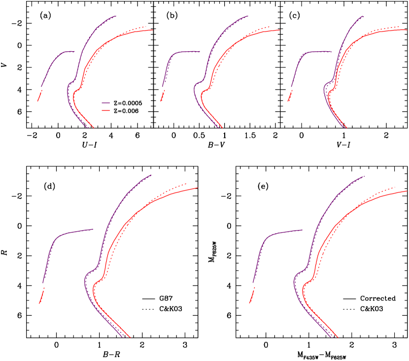
Figure 2: (a)–(d) Comparison of isochrones and ZAHB models constructed with the color–$T\rm_{eff}$ transformations by Green et al. (1987, solid lines) and by Castelli & Kurucz (2003, dotted lines). The model lines plotted are identical to the models for the most metal-poor (purple lines) and the most metal-rich (red lines) subpopulations in $\omega$ Cen (see §3.1 below). (e) Solid lines are models corrected by adding the difference between the two color transformations in (d) to the dotted lines obtained from Castelli & Kurucz (2003).

Figure 2 compares our isochrones and zero-age HB (ZAHB) models transformed by using the two different color tables. They are for the chemical compositions and ages appropriate for the most metal-poor and the most metal-rich (also helium-rich) subpopulations in $\omega$ Cen (see §3.1 below). While the models are in general agreement, there are minor but noticeable differences in the slope of the metal-rich RGB, especially in panel (d), i.e., $B-R$ color. Assuming that these differences in the Johnson-Cousins $UBVRI$ system would be similar in the adjacent passbands of the $HST$ filter system, we have applied small corrections to the synthetic magnitudes of the $HST$ ACS/WFC F435W and F625W passbands. For instance, for the F435W band, we added the differences in the $B$ band magnitudes between the two tables, to the synthetic F435W magnitudes. Similarly, we used the differences in the $R$ bands for the F625W bands. The corrected colors are compared with synthetic colors in panel (e). In case of the UV (F225W, F275W, and F336W) and the broad VI passbands (F606W and F814W) of the $HST$ WFC3/UVIS and ACS/WFC systems, the differences between the two color transformations are relatively small (see Fig. 2a and 2c), and therefore, we did not apply the corrections to these passbands. The Strömgren $b$ and $y$ bands are very similar to the Johnson $B$ and $V$ bands, and because the two color transformations agree well for the metal-poor population in $B-V$ color (see Fig. 2b), we also did not apply the corrections to these passbands. Interstellar extinctions for the filter systems used were estimated according to Cardelli et al. (1989) and Sirianni et al. (2005), based on the $E(B-V)$ values listed in the updated catalog of Harris (1996).

2.2 A Fitting Technique for Finding Best Parameters

In order to fit our synthetic models to the observed CMDs and find the values of ages, metallicities, and helium abundances of subpopulations in each GC, we have combined both eye fitting on the CMDs and $\chi^{2}$ minimization technique on the Hess diagrams. First, from the literature, we predetermined population ratio of subpopulations in a GC, metallicity ([Fe/H]) of each subpopulation, and a difference in the total CNO content ($\Delta$[CNO/Fe]) between subpopulations. Synthetic CMDs were then constructed for the relevant filter systems, and they were first compared with the observed CMDs by eye fitting. At this stage, initial guesses of age and helium abundance were assigned, and distance modulus, reddening, and [Fe/H] values of each subpopulation were fixed within the observational uncertainty.

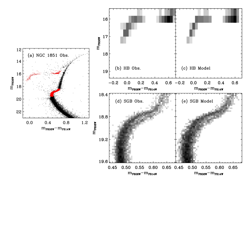
Figure 3: An example of the comparison between the observed and synthetic Hess diagrams used in our $\chi^{2}$ minimization technique for NGC 1851. (a) Red points represent CMD regions used in our $\chi^{2}$ minimization (data from Milone et al. 2008). (b)–(e) The observed and synthetic Hess diagrams for HB and SGB regions, respectively.

The best fitting values of age and helium abundance for all subpopulations were then simultaneously determined by performing a $\chi^{2}$ minimization between the observed and synthetic Hess diagrams. This was inspired by the techniques widely used in dwarf galaxy studies (e.g., Harris & Zaritsky, 2001, 2004; Tolstoy et al., 2009; Rubele et al., 2011). For example, Figures 3 and 4 illustrate our procedure for NGC 1851. Panel (a) in Figure 3 shows the CMD regions used in the $\chi^{2}$ minimization, and panels (b) and (d) display the Hess diagrams of the observed CMD. Using the predetermined parameters of each GC, we constructed a set of synthetic CMDs with an age resolution of 0.1 Gyr and helium abundance resolution of 0.01, including observational error simulations. Based on these models, synthetic Hess diagrams were produced by averaging 1000 simulations to minimize stochastic effects. The synthetic Hess diagrams were finally compared with the observed ones using the IDL function XSQ TEST, which performs the $\chi^{2}$ goodness-of-fit test between the observed and expected frequencies of a theoretical distribution. We have fixed helium abundance of the metal-poor first-generation (G1) subpopulation to be normal value (i.e., Y = Y_p + 2Z, Y_p = 0.23), so that G1 was examined only for age variation, while the metal-rich second-generation (G2) subpopulation was investigated for the variations of both age and helium abundance, simultaneously. Panels (c) and (e) in Figure 3 are the model Hess diagrams with the minimum $\chi^{2}$, and Figure 4 is the distribution of reduced $\chi^{2}$ ($\chi_{\nu}^{2}$) values for the variations in age and helium abundance of each subpopulation. The 68% (1 $\sigma$) confidence levels were calculated by bootstrapping with 1000 simulations for each subpopulation. The estimated 1 $\sigma$ errors are typically $\pm$ 0.3 Gyr for the relative age and $\pm$ 0.02 for helium abundance (Y). Note that these errors are only for the case when the metallicities and the total CNO contents are held fixed, and therefore, the actual errors would be larger if the measurement errors of metallicity and [CNO/Fe] are not negligible. The uncertainties in the distance modulus and reddening, which are fixed in the analysis, as well as those in stellar models, are also not included in the quoted errors. Note, however, that they would have only limited impact on the estimation of relative differences in age and helium abundance.

3 SYNTHETIC COLOR MAGNITUDE DIAGRAMS

3.1 $\omega$ Cen

As numerous photometric and spectroscopic studies have been devoted to it, the most massive GC, $\omega$ Cen, is indeed the most complex object among GCs in the Milky Way. It shows several prominent features in the CMDs such as a double MS, multiple subgiant branches (SGBs), multiple RGBs, and extreme blue HBs (EBHBs), as well as large variations in the spectroscopic abundance of heavy elements (Lee et al., 1999; Pancino et al., 2000; Rey et al., 2004; Ferraro et al., 2004; Bedin et al., 2004; Sollima et al., 2005a, 2006, 2007; Piotto et al., 2005; Villanova et al., 2007; Bellini et al., 2010; Freeman & Rodgers, 1975; Norris et al., 1996; Suntzeff & Kraft, 1996; Johnson & Pilachowski, 2010; Carretta et al., 2010a; Marino et al., 2011a). The multiple and discrete RGBs, together with their spectroscopic variations in the abundance of heavy elements, directly indicate that subpopulations in $\omega$ Cen were influenced by SNe. Meanwhile, the presence of a double MS and the fact that the bluer MS is more metal-rich than the redder MS strongly suggest that there is a large variation of helium abundance in this cluster (Bedin et al., 2004; Norris, 2004; Lee et al., 2005; Piotto et al., 2005). The presence of unusually extended HB is also naturally explained by the subpopulations enhanced in helium (Lee et al., 2005).

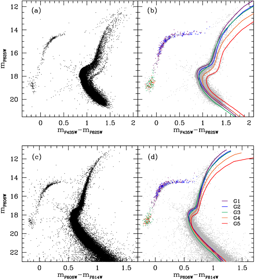
Figure 5: Comparison of our models with the observations for $\omega$ Cen. (a), (c) Observed CMDs by $HST$ ACS/WFC for the F435W, F625W and F606W, F814W passbands (data from Bellini et al. 2010). (b), (d) Our population models compared on the observed CMDs. Parameters suggested from our best simulation are listed in Table 4. Adopted distant modulus and reddening are ($m$$-$$M)_{F625W}$ = 14.03, $E(F435W$$-$$F625W$) = 0.225, and ($m$$-$$M)_{F606W}$ = 14.05, $E(F606W$$-$$F814W)$ = 0.11, respectively.

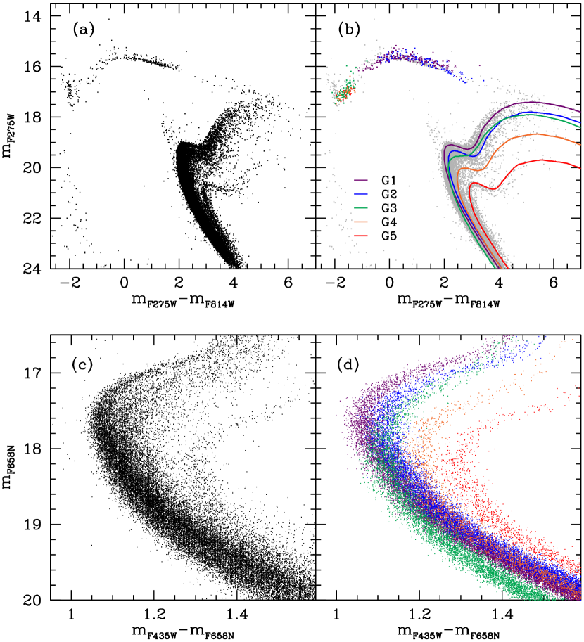
Figure 6: (a), (b) Same as Fig. 5 but for the F275W ($HST$ WFC3/UVIS) and F814W (ACS/WFC) passbands (data from Bellini et al. 2010). We can see that the model parameters obtained from the optical (F435W, F625W) bands can also reproduce the observed features from the UV (F275W) and broad $I$ (F814W) bands. (c) CMD for the MS and SGB region in the ACS/WFC F435W and F658N passbands. (d) Our synthetic models constructed with the photometric errors and total number of stars comparable to the observed CMD in panel (c). Adopted distant modulus and reddening are ($m$$-$$M)_{F275W}$ = 14.85, $E(F275W$$-$$F814W$) = 0.91, and ($m$$-$$M)_{F658N}$ = 13.97, $E(F435W$$-$$F658N)$ = 0.22, respectively.

Following the techniques and spirits employed in our previous investigation (Lee et al., 2005), we have constructed new synthetic CMDs for $\omega$ Cen. As described in §2.1, there have been two major improvements in our modeling. One is the adoption of the new Y² HB evolutionary tracks, together with the corresponding Y² isochrones, with which the enhancements in both helium abundance and [CNO/Fe] can be tested self-consistently. The other is the improvement of the color-temperature transformation including the “semi-empirical corrections” for the $HST$ ACS/WFC F435W and F625W passbands (see Fig. 2e). Furthermore, the best fitting parameters are now determined with the method described in §2.2. In the construction of synthetic CMDs, the metallicities ([Fe/H]) for the five subpopulations were first adopted from the most recent spectroscopic observations of RGB stars (Johnson & Pilachowski, 2010; Marino et al., 2011a), which are largely consistent with earlier estimates (Norris et al., 1996; Suntzeff & Kraft, 1996; Smith et al., 2000; Pancino et al., 2002; Rey et al., 2004; Sollima et al., 2005a, b; Piotto et al., 2005; Villanova et al., 2007; Johnson et al., 2008, 2009). The differences in [CNO/Fe] among the five subpopulations were taken from the recent observations by Marino et al. (2012a), and the adopted values are listed in table 2. We have then determined the best fitting ages and helium abundances by performing the $\chi^{2}$ minimization on the Hess diagrams employing the $HST$ ACS/WFC F435W and F658N passbands. In Figures 5 and 6, our synthetic models are compared with the observed CMDs by Bellini et al. (2010), and the best fitting parameters obtained by our model simulations are listed in Table 2. These model CMDs were specifically constructed to reproduce the observed CMDs, adopting the same $HST$ filter systems, population ratios, and photometric errors.

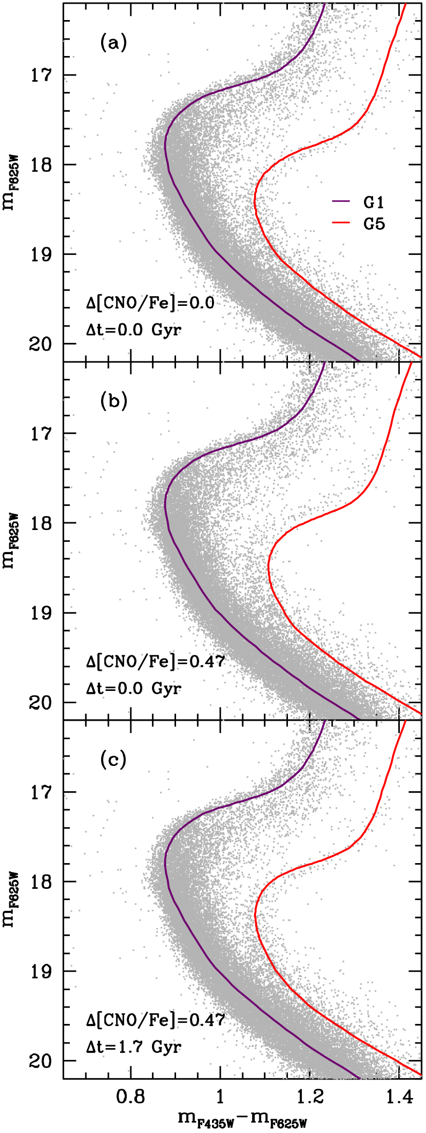
Figure 7: Similar to Fig. 5b, but here the models are constructed to illustrate the effects of $\Delta$[CNO/Fe] on the age dating. (a) If $\Delta$[CNO/Fe] = 0.0 between G1 and G5, no difference in age is obtained between them. (b), (c) When the observed $\Delta$[CNO/Fe] is included, $\Delta$t = 1.7 Gyr is required between G1 and G5, in the sense that G5 is younger, otherwise models would not match the observations.

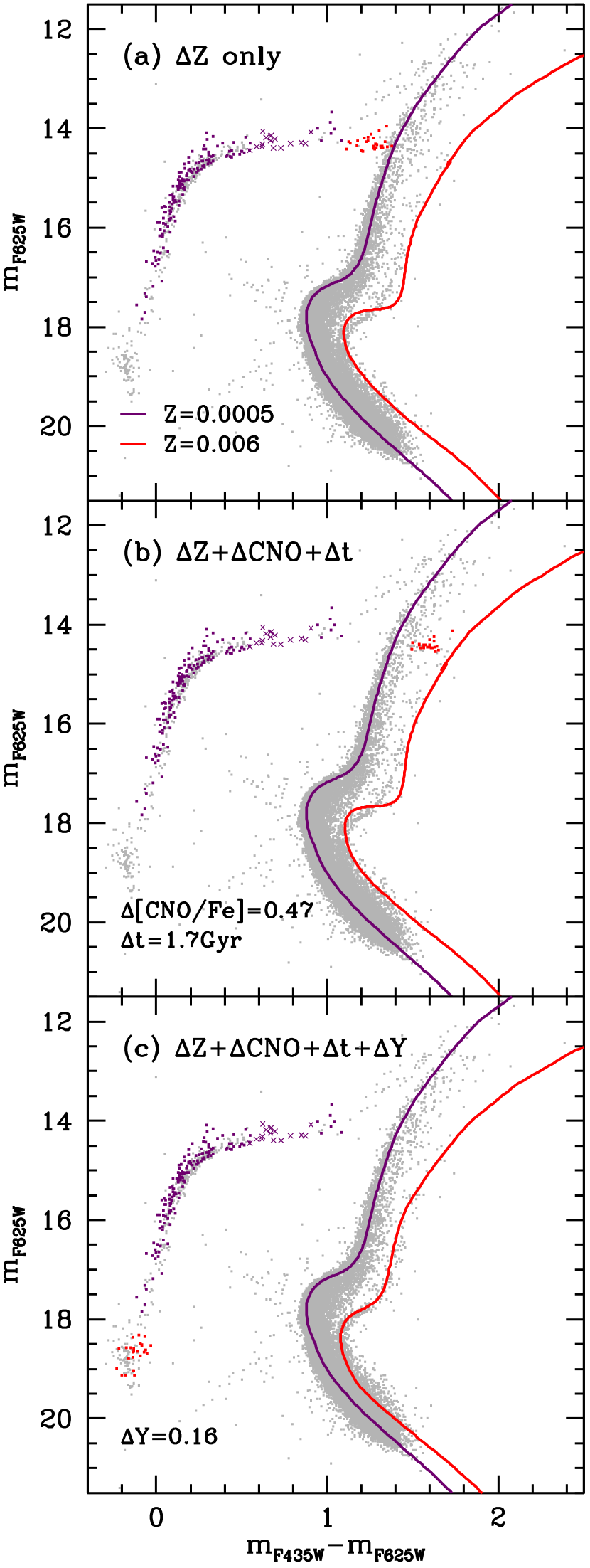
Figure 8: Similar to Fig. 5b, but here the models are constructed to illustrate, independently, the effects of metallicity, the total CNO content, age, and helium abundance on the overall morphology in the CMD (see text).

For the two most metal-poor subpopulations, which we refer to as G1 and G2, reasonable agreements with the observations, from MS to HB, are achieved with normal helium abundances (i.e., Y = Y_p + 2Z, Y_p = 0.23). The RR Lyrae stars belonging to these metal-poor subpopulations are also providing a very firm constraint ($\Delta$Y $\lesssim$ 0.01) on the helium abundance as the luminosities and periods of RR Lyraes depend very sensitively on helium abundance (see below). For the ages of these subpopulations, our fitting technique is suggesting 13.1 $\pm$ 0.2 and 13.0 $\pm$ 0.3 Gyrs, respectively, and therefore they could be coeval to within the uncertainty. For the intermediate metallicity subpopulation, G3, however, a large amount of helium enhancement ($\Delta$Y = 0.18 $\pm$ 0.02) is suggested from our fitting technique to reproduce not only the bluer and fainter MS but also the EBHB stars. This is readily understood by the effects of helium abundance in stellar astrophysics. Because of the higher core temperature and decreased envelope opacity, helium-rich stars, in general, are bluer and brighter for a given mass. Since they evolve faster than helium-poor stars, helium-rich stars would have smaller masses for a given age, and therefore the helium-rich MS appears both bluer and fainter than the helium-poor sequence on the isochrone (see, e.g., Cox & Giuli, 1968; Iben & Faulkner, 1968; Lee et al., 2005). For the same reason, helium-rich HB stars have smaller total masses than do less helium-rich stars and end up on the blue HB or EBHB (Lee et al., 1994). The best fitting age for this helium enhanced G3 is 12.0 $\pm$ 0.4 Gyr, which is about 1 Gyr younger than the reference subpopulations (G1 and G2). Similarly, for the two most metal-rich subpopulations, G4 and G5, our models require helium enhancements as much as that for G3, from the presence of EBHB stars and the round shape of the SGBs. If they were not enhanced in helium abundance, they should have red HB stars or red clumps and more flattened SGBs at their metallicities, [Fe/H] $\gtrsim$ $-$1.0 (see Fig. 8 below, Sollima et al., 2005b, see also). For these subpopulations, our fitting technique is suggesting a common age of 11.4 $\pm$ 0.4 Gyr, and therefore, the age difference between G1 and G5 is predicted to be about 1.7 $\pm$ 0.5 Gyr. This formation time scale of $\omega$ Cen has important implications for understanding the behaviors of the $\alpha$-elements and $s$-process elements (e.g., Norris & Da Costa, 1995; Busso et al., 1999; Smith et al., 2000; Johnson & Pilachowski, 2010; D’Antona et al., 2011; Marino et al., 2011a, 2012a; D’Orazi et al., 2011; Valcarce & Catelan, 2011). Note that the variation in total CNO content between the subpopulations has the most significant impact on this age difference. As shown in Figure 7, if there were no variation in [CNO/Fe], our models suggest that all of the subpopulations in $\omega$ Cen would be almost coeval (see also Marín-Franch et al., 2010; D’Antona et al., 2011; Marino et al., 2012a).

In order to illustrate, independently, the effects of metallicity, [CNO/Fe], age, and helium abundance on the overall morphology in CMD, Figure 8 compares the synthetic CMDs constructed under different combinations of these parameters. The presented models are for the metallicities comparable to the most metal-poor and the most metal-rich subpopulations in $\omega$ Cen, G1 and G5. First, the $\Delta$Z-only model in panel (a) is for the case in which G5 has enhanced metallicity but the same [CNO/Fe], age, and helium abundance with G1. The $\Delta$Z + $\Delta$CNO + $\Delta$t model in panel (b) is for the case in which [CNO/Fe] is also enhanced and age is decreased for G5. Both enhanced [CNO/Fe] and decreased age are pushing the HB of G5 to even redder color (see Lee et al., 1994), while they have opposite effects on the MS turn-off (MSTO) and SGB regions (see also Fig. 7) so that no appreciable change is seen there. Finally, $\Delta$Z + $\Delta$CNO + $\Delta$t + $\Delta$Y model in panel (c) is for the case where the helium abundance of G5 is also significantly enhanced, as in our best simulation. As is clear from Figure 8, G5 would have the red HB in the models without helium enhancement, while the enhanced helium abundance in panel (c) pushes the HB stars into the EBHB region. It is also shown that the luminosity and color of MSTO, together with the SGB slope, are fairly affected by this variation in helium abundance.

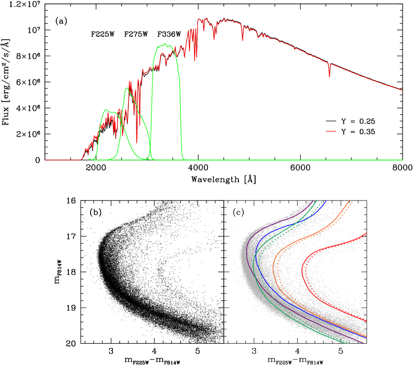
Figure 9: The effect of helium enhancement on the stellar spectra. (a) Synthetic spectra (Castelli & Kurucz, 2003) of two stars near the MSTO, with the same $T\rm_{eff}$ = 6000 K, log $g$ = 4.5, and [Fe/H] = $-$1.5, but different helium abundance (Y = 0.25 & 0.35). Green lines are filter throughputs for three UV-passbands (F225W, F275W, and F336W) of $HST$ WFC3/UVIS. (b) Observed CMD of $\omega$ Cen in F225W and ACS/WFC F814W passbands (data from Bellini et al. 2010). (c) The effect of helium-enhanced spectra on the CMD. Color codings are as in Fig. 5. The dotted lines are models from the normal helium (Y = 0.25) spectra, while solid lines are those from the helium-enhanced (Y = 0.38$-$0.41) spectra. Adopted distant modulus and reddening are ($m$$-$$M)_{F814W}$ = 13.9 and $E(F225W$$-$$F814W$) = 1.26, respectively.

In our modeling, the effects of enhancements in helium and the total CNO abundances were only considered in the stellar interior, and it was assumed that their effects on stellar atmosphere would be negligible. For the effect of helium abundance, we have confirmed this using the helium-enhanced model fluxes of Castelli & Kurucz (2003). Figure 9a shows the model spectra of two stars with different helium abundances ($\Delta Y$ = 0.10) but the same temperature, gravity, and metallicity (i.e., $T\rm_{eff}$ = 6000 K, log $g$ = 4.5, and [Fe/H] = $-$1.5), which correspond roughly to stars near the MSTOs of G2 and G3 in $\omega$ Cen. We can see that a large variation in helium abundance ($\Delta Y$ = 0.10) has only negligible effect on stellar atmosphere (see also Girardi et al., 2007; Sbordone et al., 2011). In the UV region, for the wavelengths shorter than $\sim$4000 Å, however, some differences between the two synthetic spectra are noticed. Figure 9c shows that, in the worst situation, combinations of $T\rm_{eff}$, log $g$, [Fe/H], and the helium variations of $\Delta Y$ = 0.10 can make differences in magnitude up to $\sim$0.15 in the UV bands. In the case of the total CNO abundance, our assumption appears to be valid also in the optical passbands. Using synthetic spectra, Sbordone et al. (2011) have shown that the variations in C, N, O, and Na abundances mainly affect wavelengths shorter than $\sim$4000 Å. They have also reported that the effect on the $hk$ index is negligible (at most $\sim$0.04 mag), while CMDs including $U$ band could be affected by $\sim$0.2–0.3 mag for the $\sim$0.3 dex variation in [CNO/Fe]. Considering these uncertainties in the UV regime, the best fitting parameters in our models are determined based only on the optical bands and the $hk$ index.

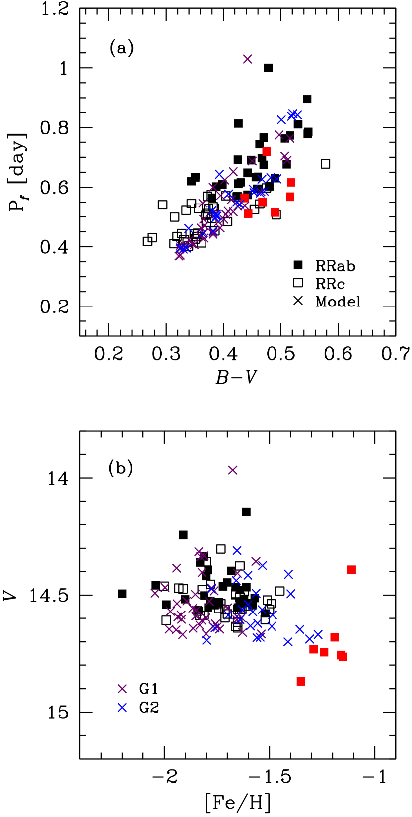
Figure 10: Comparison of the observed RR Lyrae variables (squares) in $\omega$ Cen with the synthetic HB models (crosses). Red squares are metal-rich RRab stars ([Fe/H] $>$ $-$1.4). RR Lyrae data from Sollima et al. (2006) and Kaluzny et al. (2004). Purple and blue crosses are model RR Lyrae stars from G1 and G2, respectively. This suggests that there is an additional minor subpopulation between G2 and G3, having normal helium-abundance and [Fe/H] $\approx$ $-$1.3. Adopted distant modulus and reddening are ($m$$-$$M)_{V}$ = 14.1 and $E(B$$-$$V$) = 0.14, respectively (see text).

Some HB stars in our models are in the RR Lyrae instability strip, and they can provide additional constraints in the modeling. Following Lee et al. (1990), we have computed the fundamental periods (P_f), using the equation of stellar pulsation (van Albada & Baker, 1971), for the RR Lyrae candidates in the synthetic HB. Figure 10 compares our synthetic stars to the observed RR Lyrae variables in $\omega$ Cen, where the metallicities of 74 RR Lyrae stars are from the spectroscopic measurements by Sollima et al. (2006). In panel (a), the periods of $c$-type RR Lyrae stars are fundamentalized assuming the period ratio, P_c/P_ab = 0.745, between the $c$-type and $ab$-type RR Lyare stars (Clement et al., 2001; Alcock et al., 2000). In our models, only the two most metal-poor subpopulations, G1 and G2, have RR Lyrae stars. The HB stars from the three metal-rich and super-helium-rich subpopulations, G3, G4, and G5, are too hot to produce RR Lyare stars as they are on the EBHB region far beyond the blue edge of the instability strip. In panel (b), metallicities of the synthetic RR Lyrae stars have been assigned randomly according to a Gaussian distribution centered on the metallicities of the G1 and G2 (see Table 2), respectively, with $\sigma_{[Fe/H]}$ = 0.13, which is roughly consistent with the observational error in [Fe/H] measurement. The predicted periods, $\it V$ magnitudes, and [Fe/H] from our model populations, G1 and G2, show good agreements with the observed RR Lyrae variables except for the several stars having intermediate metallicity ($-$1.4 $<$ [Fe/H] $<$ $-$1.0). As pointed out by Sollima et al. (2006), these stars are expected to have normal helium abundance because their luminosities and periods are not increased (see Lee et al., 1994). This implies that a minor subpopulation having a similar metallicity but different helium abundance with G3 may coexist in $\omega$ Cen. The presence of these normal-helium, intermediate metallicity RR Lyrae stars, together with the $HST$ WFC3 UV photometry by Bellini et al. (2010), suggests that $\omega$ Cen contains additional minor subpopulations between the five subpopulations adopted in this study.

3.2 M22

It has long been suspected that RGB stars in the massive GC M22 show a spread in heavy element abundance, but the presence of differential reddening, caused by its location near the Galactic plane, has prevented a firm confirmation of its reality (e.g., Hesser et al., 1977; Pilachowski et al., 1982; Norris & Freeman, 1983; Lehnert et al., 1991; Anthony-Twarog et al., 1995; Monaco et al., 2004; Ivans et al., 2004). Recent observations, however, have shown that M22 indeed hosts two stellar subpopulations differing in the abundance of heavy elements. Based on high resolution spectroscopy, Marino et al. (2009, 2011b) identified two stellar groups separated by $\sim$0.15 dex in [Fe/H], while Da Costa et al. (2009) reported a somewhat larger difference in metallicity ($\sim$0.26 dex). Meanwhile, J.-W. Lee et al. (2009a) has clearly shown that M22 has a discrete double RGB having different Ca abundance from the $hk$ index of the Ca-by photometry.

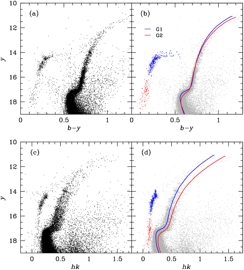
Figure 11: Comparison of our models with the observations for M22. (a), (c) Strömgren $b$, $y$, and calcium ($Ca$) narrow-band photometry from S.-I. Han et al. (2012, in preparation), where the $hk$ index is defined as $hk$ = $(Ca-b)-(b-y)$. (b), (d) Our population models compared on the observed CMDs. Adopted distant modulus and reddening are ($m$$-$$M)_{y}$ = 13.80, $E(b$$-$$y$) = 0.255, and $E(hk)$ = $-$0.012.

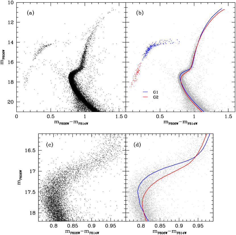
Figure 12: Comparison of our models with the observations for M22. (a) Observed CMD by $HST$ ACS/WFC for the F606W and F814W passbands. Photometric data from the ACS survey (Sarajedini et al., 2007; Anderson et al., 2008). (b) Our models compared on the observed CMD. (c), (d) Same as (a) & (b) but zoomed in for the SGB region. A clearer view of the SGB split can be seen in Milone et al. (2010, see their Fig. 2). Adopted distant modulus and reddening are ($m$$-$$M)_{F606W}$ = 13.69 and $E(F606W$$-$$F814W$) = 0.355, respectively.

In the left panels of Figure 11, we show CMDs of M22 from S.-I. Han et al. (2012, in preparation), which were observed with the Strömgren $b$, $y$ and a new narrow band calcium filter specially designed to avoid a possible contamination from the adjacent CN bands. We can see two well-separated RGBs in the $hk$ index, which are very similar to those in Figure 1 of J.-W. Lee et al. (2009a), and a bimodal distribution of HB stars composed of blue HB and EBHB. Based on these photometric data and the CMD from the ACS survey (Piotto, 2009), shown in Figure 12a, we constructed synthetic CMDs as described in §2. The difference in [CNO/Fe] between the two subpopulations was adopted to be 0.13 dex from the recent observations (Marino et al., 2011b, 2012b, see also Alves-Brito et al., 2012).

The right panels of Figures 11 and 12 are the final outcomes of our population models compared with the observed CMDs. The best fitting model parameters are listed in Table 3. The metal-poor subpopulation, which we refer to as the first-generation (G1) population, contains the bluer RGB, brighter SGB, and blue HB stars, while the metal-rich subpopulation, which we refer to as the second-generation (G2) population, has the redder RGB, fainter SGB, and EBHB stars. In order to simultaneously reproduce these observed splits on the RGB and SGB, and the bimodal HB distribution, we need a small but important difference in metallicity ($\Delta$[Fe/H] = 0.25 dex), and at the same time, a large difference in helium abundance ($\Delta$Y = 0.09 $\pm$ 0.04) between the two subpopulations. By applying a small difference in the total CNO content ($\Delta$[CNO/Fe] = 0.13 dex; Marino et al. 2012b), our models suggest that the best fitting age difference is very small ($\Delta$t = 0.3 $\pm$ 0.4 Gyr). The adopted difference in metallicity is similar to the observed difference obtained from Ca II triplet ($\sim$0.26 dex; Da Costa et al. 2009), while it is somewhat larger than the difference obtained from [Fe/H] ($\sim$0.15 dex; Marino et al. 2009, 2011b). This is probably due to a small increase in calcium abundance ($\Delta$[Ca/Fe] $\approx$ 0.1; Marino et al. 2009, 2011b) in the metal-rich subpopulation, G2. Our models are also consistent with the recent spectroscopic measurements by Marino et al. (2012b), which have shown that stars in the faint SGB are more metal-rich compared to the stars in the bright SGB.

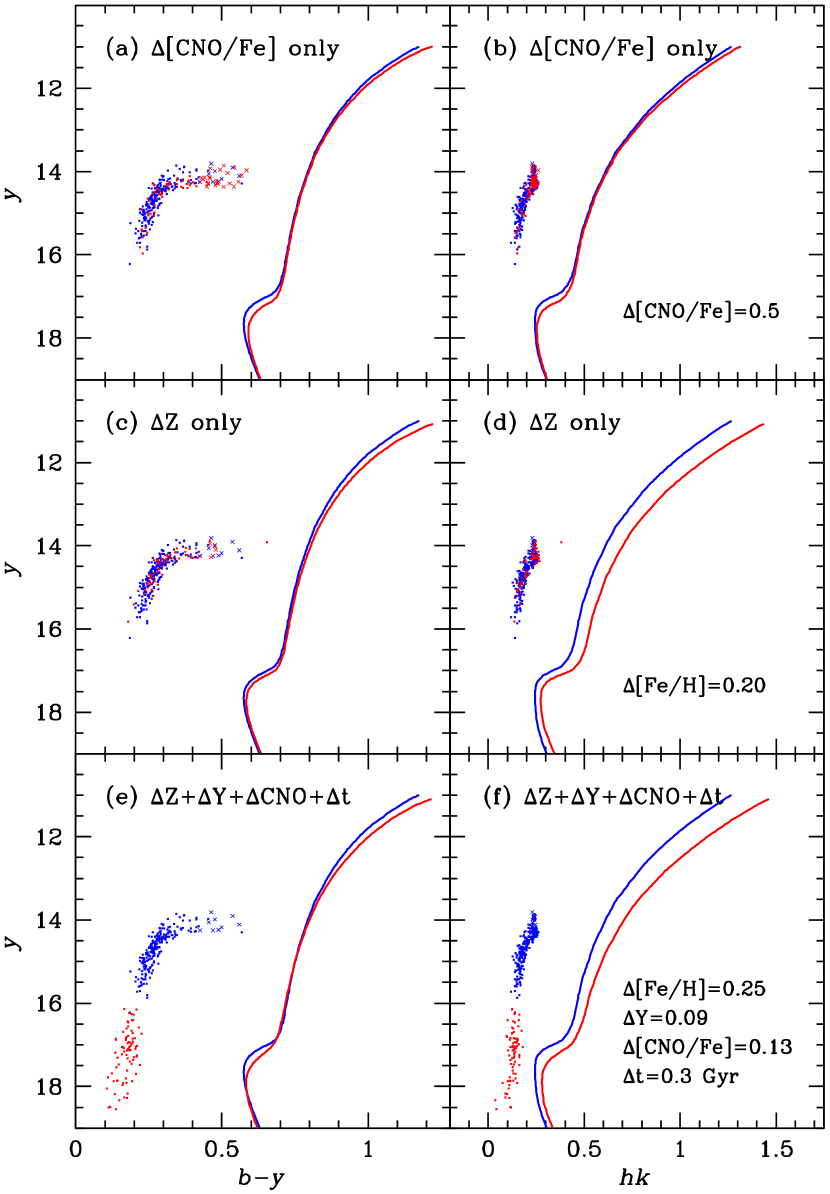
Figure 13: The effects of variations in the total CNO abundance, metallicity, and helium abundance in our models for M22 (see text).

Figure 13 explains the effects of variations in the total CNO abundance, overall metallicity, and helium abundance, independently. If we assume only the difference in [CNO/Fe] between the two subpopulations, to reproduce the split on the SGB, as suggested for NGC 1851 (Cassisi et al., 2008; Salaris et al., 2008), our models fail to explain the presence of the RGB split in the $hk$ index and the EBHB stars (the upper panels). Note that, for illustrative purpose, we have increased the difference to 0.5 dex from the observed value ($\sim$0.13 dex), because the observed difference is too small to reproduce the SGB split. Similarly, with the assumption of enhancement only in [Fe/H], our model for G2 also fails to reproduce the EBHB stars, while the split on the RGB can be explained (the middle panels). This is a natural consequence of the metallicity effect, as the HB morphology is getting redder with increasing metallicity (see, e.g., Lee et al., 1994). While this difference in [Fe/H] reproduces some split on the SGB, it is not sufficient to explain the observed difference. The bottom panels of Figure 13 show that additional enhancement in helium is needed to overcome the effect of metallicity on the HB and to reproduce the EBHB stars, as already explained in §3.1. Similarly to the case of $\omega$ Cen, this enhancement of helium also helps to reproduce the observed split on the SGB (see Fig. 12d).

The argument based on the population ratio further supports our hypothesis that the EBHB stars belong to the metal-rich subpopulation G2. The number ratio between the bluer and redder RGBs in Figure 11c and those in J.-W. Lee et al. (2009a) is about 0.7:0.3. Piotto (2009) and Marino et al. (2009) have also suggested a similar number ratio (0.62:0.38) between the bright and faint SGBs. Within the error, this is also consistent with the ratio of the EBHB stars which comprise roughly 25% of all HB stars in panel (a) of Figures 11 and 12. This would then suggest that the bright SGB, bluer RGB, and blue HB stars are all associated with the majority, metal-poor subpopulation (G1), while the faint SGB and redder RGB stars are progenitors of the EBHB stars, associated with the minority metal-rich subpopulation (G2).

3.3 NGC 1851

Recent observations of NGC 1851, which is well-known for its unusual bimodal HB distribution (e.g., Saviane et al., 1998; Walker, 1998), indicate that it also belongs to the peculiar group of massive GCs influenced by SNe enrichment like $\omega$ Cen and M22. Not only a double RGB has been revealed from several photometric observations (J.-W. Lee et al., 2009a, b; Han et al., 2009; Carretta et al., 2011a), but also some spreads in [Fe/H] have been reported from spectroscopic observations (Carretta et al., 2010c, 2011b). NGC 1851 also shows other signatures for the presence of two subpopulations, such as a double SGB (Milone et al., 2008), a CN bimodality (Hesser et al., 1982), and variations in light and $s$-process element abundances (Yong & Grundahl, 2008; Yong et al., 2009; Villanova et al., 2010; Carretta et al., 2011b). The origin of the observed SGB split, together with its possible links to the RGB split and the bimodal HB distribution, however, is still under debate. For instance, the SGB spilt can be explained by a difference in age of $\sim$1–1.5 Gyr (Milone et al., 2008; Carretta et al., 2010c, 2011b; Gratton et al., 2012b), by an increase of total CNO abundance by a factor of $\sim$2–4 (Cassisi et al., 2008; Salaris et al., 2008; Yong et al., 2009; Ventura et al., 2009; D’Antona et al., 2009), or by a combined effect of the differences in overall metallicity ($\Delta$[Fe/H] $\approx$ 0.15 dex) and helium abundance ($\Delta$Y $\approx$ 0.05; Han et al., 2009).

Based on the framework of our previous modeling (Han et al., 2009), we have constructed new synthetic CMDs for NGC 1851. The best fitting parameters were determined with the technique described in §2.2. In the case of NGC 1851, there is still no general consensus on the observed value of $\Delta$[CNO/Fe] between the two subpopulations (Yong et al., 2009; Villanova et al., 2010; Lardo et al., 2012), but Gratton et al. (2012b) recently concluded that the difference in [CNO/Fe] is less than 0.2 dex. Considering this and the similarity of NGC 1851 with M22, here, we have adopted 0.1 dex for $\Delta$[CNO/Fe]. Given the small value, this should have only a little effect in our modeling.

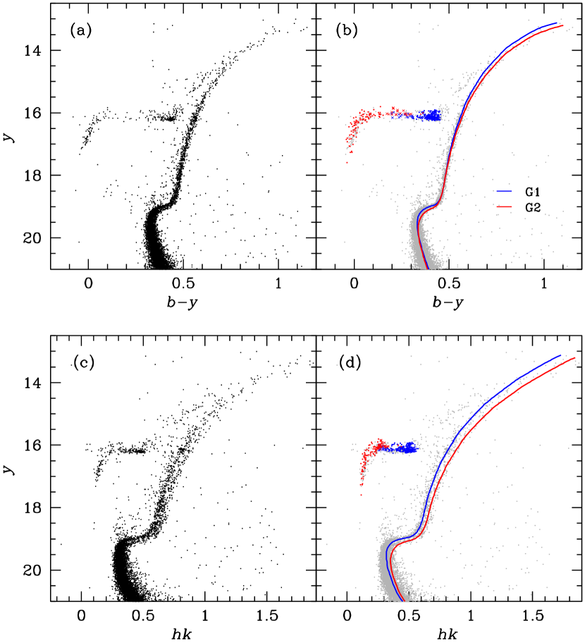
Figure 14: Same as Fig. 11, but for NGC 1851 (data from S.-I. Han et al. 2012, in preparation). Adopted distant modulus and reddening are ($m$$-$$M)_{y}$ = 15.62, $E(b$$-$$y$) = 0.015, and $E(hk)$ = $-$0.015.

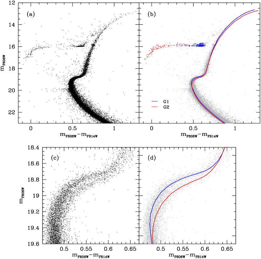
Figure 15: Same as Fig. 12, but for NGC 1851. Data from the ACS survey (Milone et al., 2008). A clearer view of the SGB split can be seen in Milone et al. (2010, see their Fig. 2). Adopted distant modulus and reddening are ($m$$-$$M)_{F606W}$ = 15.52 and $E(F606W$$-$$F814W$) = 0.025, respectively.

In Figure 14, our models are compared with new CMDs of NGC 1851, obtained from Ca-by photometry (S.-I. Han et al. 2012, in preparation). This observation confirms the previously reported split of the RGB in the $hk$ index (J.-W. Lee et al., 2009a, b). Similarly, Figure 15 compares our models with the CMDs from the ACS survey (Milone et al., 2008). The model parameters determined by our fitting technique are listed in Table 4. With the small variations in metallicity ($\Delta$[Fe/H] = 0.13 dex) and the total CNO content ($\Delta$[CNO/Fe] = 0.1 dex) between the two subpopulations, our fitting technique suggests that the difference in helium abundance is considerable ($\Delta$Y = 0.06 $\pm$ 0.01), while the difference in age is relatively small ($\Delta$t = 0.5 $\pm$ 0.2 Gyr). This result is qualitatively similar to the case of M22. The faint SGB can be explained mostly by the combined effects of the metallicity and helium enhancements, as both of them make MSTOs fainter (Fig. 15), while the small variations in the total CNO abundance and age have only little impact on the CMD. In particular, as discussed above (Fig. 7), the total CNO content and age basically affect MSTOs in opposite directions. If there were no difference in [CNO/Fe] between G1 and G2, then the age difference would be even smaller ($\Delta$t $\approx$ 0.0 Gyr). The Ca-strong redder RGB in the $hk$ index can be accounted for solely by the effect of metal enhancement, which makes RGBs redder (bottom panels of Fig. 14). The helium enhancement slightly moves the RGB to the opposite direction, but the effect of metal enrichment is far more important. In the HB region, the effect of helium enhancement, which makes HB morphology bluer, easily overcomes the effects of metallicity and CNO contents (see Fig. 13), and therefore the presence of blue HB, populated by G2, can be explained. Note that our model for G2 is also consistent with recent measurement of helium abundances for the blue HB stars (Y = 0.29 $\pm$ 0.05; Gratton et al., 2012b).

Our models indicate, therefore, that the majority subpopulation, G1, comprises the metal-poor bright SGB, Ca-weak bluer RGB, and red HB stars; while the minority subpopulation, G2, is associated with the metal-rich faint SGB, Ca-strong redder RGB, and blue HB stars. This is consistent with the population ratios estimated from Figures 14 and 15. The number fraction between the bright and faint SGBs is roughly 0.68:0.32 (Fig. 15c), and the ratio between the bluer and redder RGBs is about 0.71:0.29 (Fig. 14c). This also agrees with the number ratios reported in previous works (Milone et al., 2008, 2009; J.-W. Lee et al., 2009a; Han et al., 2009), to within the uncertainty. The ratio between the red and blue HBs is about 0.69:0.31 (Fig. 14a and Fig. 15a), if RR Lyrae stars belong to metal-poor subpopulation (G1). Note that the mean period of RR Lyrae stars ($<$P_f$>$ = 0.531 day), which is normal for the metallicity of NGC 1851 (Walker, 1998; Clement et al., 2001), also indicates that most of the RR Lyrae variables come from the majority subpopulation (G1) having normal helium abundance.

4 DISCUSSION

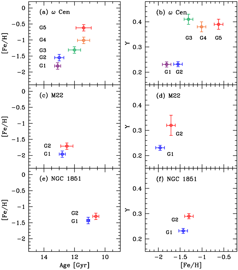
Figure 16: Schematic illustrations for the star formation histories and accompanying enrichments of metallicity and helium abundance in three GCs considered in this paper. The formation time scales of all subpopulations appear to be $\sim$1.7 Gyr for $\omega$ Cen and less than 1 Gyr for M22 and NGC 1851. Metal-rich subpopulations in these GCs are also enhanced in helium abundance. There is a dramatic increase of helium abundance between G2 and G3 in $\omega$ Cen. One sigma error bars for age and helium abundance are from our $\chi^{2}$ minimization, while the uncertainty in [Fe/H] is assumed to be 0.1 dex.

We have compared our models with the observations of three peculiar GCs, $\omega$ Cen, M22, and NGC 1851, to estimate ages, metallicities, and helium abundances of their subpopulations. Based on our results, in Figure 16, we schematically illustrate the star formation histories and accompanying enrichments of metallicity and helium abundance in these stellar systems. We find that the age differences between the metal-rich and metal-poor subpopulations in these GCs are relatively small, $\sim$0.3–1.7 Gyr, and metal-rich subpopulations with redder RGBs are also enhanced in helium abundance. The formation time scale of stellar populations in these GCs is therefore expected to be fairly short, i.e., $\sim$1.7 Gyr for $\omega$ Cen and less than 1 Gyr for M22 and NGC 1851.

How this could be understood in terms of their formation origin? The most natural assumption would be that they are self-enriched, in which later generations of stars formed from the gas enriched by the ejecta of massive stars in earlier generations. As for the sources of chemical enrichment and pollution in these GCs, at least three viable mechanisms have been proposed thus far. The explosion of type II SNe is required for the enrichments of heavy elements (Timmes et al., 1995) and perhaps helium (Norris, 2004; Piotto et al., 2005), while winds from the FRMSs and IMAGBs are suggested for the pollution of light elements and the enhancement of helium (Decressin et al., 2007; D’Antona & Ventura, 2007; Ventura & D’Antona, 2008). The enhancement of the total CNO abundance in the metal-rich later generation subpopulations would also indicate the contribution by type II SNe (see also Marino et al., 2012a). Considering the order of time required to emerge for these mechanisms, a possible scenario would be as follows: (1) Formation of the first-generation metal-poor (bluer RGB) stars from the gas having normal helium and light element abundances. (2) Pollution of the remaining gas by the winds from FRMSs, which enhance helium and alter the abundance profile of light elements. (3) The most massive ($\gtrsim$ 8 M_⊙) stars then would explode as type II SNe, enriching overall metallicity, including heavy elements and the total CNO content. (4) Further pollution of the gas by the ejecta from IMAGB stars ($\sim$3–7 M_⊙) would follow, which enhance helium and change light element abundances. (5) Finally, formation of the second-generation metal-rich (redder RGB) stars from the gas now enriched in overall metallicity and helium and polluted in light element abundances. While this scenario can naturally explain the presence of metal-rich and helium-enhanced subpopulations in these GCs, this requires that they were much more massive in the past, because their present masses are too small to retain the ejecta of SNe explosions (e.g., Dopita & Smith, 1986; Baumgardt et al., 2008). This suggests that these GCs were once nuclei of primeval dwarf galaxies and then merged and dissolved in the proto-Galaxy, as is widely accepted for $\omega$ Cen (e.g., Lee et al., 1999; Bekki & Freeman, 2003; Piotto et al., 2005; Meza et al., 2005; Lee et al., 2007; J.-W. Lee et al., 2009a; Baumgardt et al., 2008; Ferraro et al., 2009; Pflamm-Altenburg & Kroupa, 2009; Cohen et al., 2010; Bekki, 2012, and references therein). Note that a significant fraction ($\sim$30%) of the helium-enhanced subpopulation in these GCs is also best explained if the second generation stars were formed from enriched gas trapped in the deep gravitational potential well of the ancient dwarf galaxies (Bekki & Norris, 2006).

Recently, Carretta et al. (2010c, 2011b) and Bekki & Yong (2012) suggested that NGC 1851 might have formed by simple merging of two GCs having different heavy element abundances initially belonged to a proto-dwarf galaxy. While this scenario can explain the presence of RGB split and the spread in heavy element abundance without assuming self-enrichment, this is not easily reconciled with one of our main results, which suggests that the metal-rich subpopulation is also enhanced in helium abundance. In this scenario, it would be difficult to understand why all stars in initially more metal-rich GCs were selectively enhanced in helium abundance, while those in metal-poor GCs were not. Note, however, that this merging scenario might be able to explain the absence of helium enhancement between G1 and G2 in $\omega$ Cen (see §3.1), where G1 and G2 formed by simple merging of two GCs in the central part of a proto-dwarf galaxy, while more metal-rich and helium-enhanced subpopulations, G3, G4, and G5, formed later from the enriched gas trapped in the core of this merged stellar system in a proto-dwarf galaxy. Despite many uncertainties, all of the above scenarios are possible only in the primeval dwarf galaxy environment, and therefore, dwarf galaxy origin of these GCs appears to be inevitable.

Table 1: Model Ingredients

Ingredient	References
Isochrones from MS to RGB	Yonsei–Yale (Y2) isochrones (Yi et al. 2008; Y.-W. Lee et al. 2012, in preparation)
HB evolutionary tracks	Yonsei–Yale (Y2) HB tracks (Y.-W. Lee et al. 2012, in preparation)
Color–$T\rm_{eff}$ transformation	Green et al. (1987) color table
	Castelli & Kurucz (2003) model atmosphere

Table 2: Parameters suggested from our best simulation of $\omega$ Cen

Population	$Z$	[Fe/H]	$\Delta$[CNO/Fe]	$Y$	Age(Gyr)	Mass-loss($M_{\odot}$)	Fraction	other name
G1	0.0005	$-$1.81	0.0	0.231	13.1 $\pm$ 0.2	0.199	0.42	RGB-MP
G2	0.0009	$-$1.55	0.0	0.232	13.0 $\pm$ 0.3	0.217	0.28	RGB-MInt1
G3	0.0015	$-$1.31	0.14	0.41 $\pm$ 0.02	12.0 $\pm$ 0.4	0.171	0.17	RGB-MInt2
G4	0.0057	$-$1.01	0.47	0.38 $\pm$ 0.02	11.4 $\pm$ 0.4	0.220	0.08	RGB-MInt3
G5	0.0136	$-$0.62	0.47	0.39 $\pm$ 0.02	11.4 $\pm$ 0.5	0.251	0.05	RGB-a

Table 3: Parameters suggested from our best simulation of M22

Population	$Z$	[Fe/H]	$\Delta$[CNO/Fe]	$Y$	Age(Gyr)	Mass-loss($M_{\odot}$)	Fraction
G1	0.00035	$-$1.96	0.0	0.231	12.8 $\pm$ 0.2	0.189	0.7
G2	0.00067	$-$1.71	0.13	0.32 $\pm$ 0.04	12.5 $\pm$ 0.4	0.192	0.3

Table 4: Parameters suggested from our best simulation of NGC 1851

Population	$Z$	[Fe/H]	$\Delta$[CNO/Fe]	$Y$	Age(Gyr)	Mass-loss($M_{\odot}$)	Fraction
G1	0.0012	$-$1.43	0.0	0.232	11.1 $\pm$ 0.1	0.208	0.7
G2	0.0018	$-$1.30	0.10	0.29 $\pm$ 0.01	10.6 $\pm$ 0.2	0.212	0.3

Figure 1: Calibration of the Reimers (1977) mass-loss coefficient, $\eta$, on the HB morphology vs. [Fe/H] relation. Data for the inner halo (R_GC $<$ 8 kpc) GCs from Lee et al. (1994, 2007). Solid lines are theoretical isochrones produced by our synthetic HB models for 13 Gyr using $\eta$ = 0.46, 0.53, and 0.60, respectively. Two metal-rich GCs with extended HB are marked and are excluded in the comparison.

Figure 4: Distributions of reduced $\chi^{2}$ ($\chi_{\nu}^{2}$) values in the fitting of our models with the observed Hess diagram for NGC 1851. For the first-generation (G1) population, only age is examined, while for the second-generation (G2) population, both age and helium abundance (Y) are simultaneously investigated to find the values with minimum $\chi^{2}$. In panel (b), the values of $\chi_{\nu}^{2}$ are listed on the contour map (see text).

References

- Alcock et al. (2000) Alcock, C., Allsman, R., Alves, D. R., et al. 2000, ApJ, 542, 257
- Alves-Brito et al. (2012) Alves-Brito, A., Yong, D., Meléndez, J., Vásquez, S., & Karakas, A. I. 2012, A&A, 540, A3
- Anderson et al. (2008) Anderson, J., Sarajedini, A., Bedin, L. R., et al. 2008, AJ, 135, 2055
- Anthony-Twarog et al. (1995) Anthony-Twarog, B. J., Twarog, B. A., & Craig, J. 1995, PASP, 107, 32
- Anthony-Twarog et al. (1991) Anthony-Twarog, B. J., Twarog, B. A., Laird, J. B., & Payne, D. 1991, AJ, 101, 1902
- Baumgardt et al. (2008) Baumgardt, H., Kroupa, P., & Parmentier, G. 2008, MNRAS, 384, 1231
- Bedin et al. (2005) Bedin, L. R., Cassisi, S., Castelli, F., Piotto, G., Anderson, J., Salaris, M., Momany, Y., & Pietrinferni, A. 2005, MNRAS, 357, 1038
- Bedin et al. (2004) Bedin, L. R., Piotto, G., Anderson, J., Cassisi, S., King, I. R., Momany, Y., & Carraro, G. 2004, ApJ, 605, L125
- Bekki (2012) Bekki, K. 2012, MNRAS, 421, L44
- Bekki & Freeman (2003) Bekki, K., & Freeman, K. C. 2003, MNRAS, 346, L11
- Bekki & Norris (2006) Bekki, K., & Norris, J. E. 2006, ApJ, 637, L109
- Bekki & Yong (2012) Bekki, K., & Yong, D. 2012, MNRAS, 419, 2063
- Bellini et al. (2010) Bellini, A., Bedin, L. R., Piotto, G., Milone, A. P., Marino, A. F., & Villanova, S. 2010, AJ, 140, 631
- Bessell (1990a) Bessell, M. S. 1990a, PASP, 102, 1181
- Bessell (1990b) Bessell, M. S. 1990b, A&AS, 83, 357
- Bessell et al. (1998) Bessell, M. S., Castelli, F., & Plez, B. 1998, A&A, 333, 231
- Böker (2008) Böker, T. 2008, ApJ, 672, L111
- Busso et al. (1999) Busso, M., Gallino, R., & Wasserburg, G. J. 1999, ARA&A, 37, 239
- Cardelli et al. (1989) Cardelli, J. A., Clayton, G. C., & Mathis, J. S. 1989, ApJ, 345, 245
- Carretta et al. (2011a) Carretta, E., Bragaglia, A., Gratton, R., D’Orazi D’Orazi, V., & Lucatello, S. 2011a, A&A, 535, A121
- Carretta et al. (2009a) Carretta, E., Bragaglia, A., Gratton, R., & Lucatello, S. 2009a, A&A, 505, 139
- Carretta et al. (2010a) Carretta, E., Bragaglia, A., Gratton, R. G., et al. 2010a, ApJ, 714, L7
- Carretta et al. (2009b) Carretta, E., Bragaglia, A., Gratton, R. G., et al. 2009b, A&A, 505, 117
- Carretta et al. (2010b) Carretta, E., Bragaglia, A., Gratton, R. G., et al. 2010b, A&A, 516, A55
- Carretta et al. (2010c) Carretta, E., Gratton, R. G., Lucatello, S., et al. 2010c, ApJ, 722, L1
- Carretta et al. (2011b) Carretta, E., Lucatello, S., Gratton, R. G., Bragaglia, A., & D’Orazi, V. 2011b, A&A, 533, A69
- Cassisi et al. (2008) Cassisi, S., Salaris, M., Pietrinferni, A., et al. 2008, ApJ, 672, L115
- Castelli & Kurucz (2003) Castelli, F., & Kurucz, R. L. 2003, in IAU Symp. 210, Modelling of Stellar Atmospheres, ed. N. Piskunov, W. W. Weiss, & D. F. Gray (San Francisco: ASP), 20
- Clement et al. (2001) Clement, C. M., Muzzin, A., Dufton, Q., et al. 2001, AJ, 122, 2587
- Cohen et al. (2010) Cohen, J. G., Kirby, E. N., Simon, J. D., & Geha, M. 2010, ApJ, 725, 288
- Cox & Giuli (1968) Cox, J. P., & Giuli, R. T. 1968, Principles of Stellar Structure (New York: Gordon and Breach)
- Crawford & Barnes (1970) Crawford, D. L., & Barnes, J. V. 1970, AJ, 75, 978
- Da Costa et al. (2009) Da Costa, G. S., Held, E. V., Saviane, I., & Gullieuszik, M. 2009, ApJ, 705, 1481
- D’Antona & Caloi (2004) D’Antona, F., & Caloi, V. 2004, ApJ, 611, 871
- D’Antona et al. (2011) D’Antona, F., D’Ercole, A., Marino, A. F., et al. 2011, ApJ, 736, 5
- D’Antona et al. (2009) D’Antona, F., Stetson, P. B., Ventura, P., et al. 2009, MNRAS, 399, L151
- D’Antona & Ventura (2007) D’Antona, F., & Ventura, P. 2007, MNRAS, 379, 1431
- Decressin et al. (2007) Decressin, T., Meynet, G., Charbonnel, C., Prantzos, N., & Ekström, S. 2007, A&A, 464, 1029
- di Criscienzo et al. (2011) di Criscienzo, M., D’Antona, F., Milone, A. P., et al. 2011, MNRAS, 414, 3381
- Dopita & Smith (1986) Dopita, M. A., & Smith, G. H. 1986, ApJ, 304, 283
- D’Orazi et al. (2011) D’Orazi, V., Gratton, R. G., Pancino, E., et al. 2011, A&A, 534, A29
- Dotter et al. (2007) Dotter, A., Chaboyer, B., Jevremović, D., Baron, E., Ferguson, J. W., Sarajedini, A., & Anderson, J. 2007, AJ, 134, 376
- Dotter et al. (2010) Dotter, A., Sarajedini, A., Anderson, J., et al. 2010, ApJ, 708, 698
- Dupree et al. (2011) Dupree, A. K., Strader, J., & Smith, G. H. 2011, ApJ, 728, 155
- Ferraro et al. (2009) Ferraro, F. R., Dalessandro, E., Mucciarelli, A., et al. 2009, Nature, 462, 483
- Ferraro et al. (2004) Ferraro, F. R., Sollima, A., Pancino, E., Bellazzini, M., Straniero, O., Origlia, L., & Cool, A. M. 2004, ApJ, 603, L81
- Freeman & Rodgers (1975) Freeman, K. C., & Rodgers, A. W. 1975, ApJ, 201, L71
- Girardi et al. (2007) Girardi, L., Castelli, F., Bertelli, G., & Nasi, E. 2007, A&A, 468, 657
- Gnedin et al. (2002) Gnedin, O. Y., Zhao, H., Pringle, J. E., et al. 2002, ApJ, 568, L23
- Gratton et al. (2012a) Gratton, R. G., Carretta, E., & Bragaglia, A. 2012a, A&A Rev., 20, 50
- Gratton et al. (2012b) Gratton, R. G., Lucatello, S., Carretta, E., et al. 2012b, A&A, 539, A19
- Green et al. (1987) Green, E. M., Demarque, P., & King, C. R. 1987, The Revised Yale Isochrones & Luminosity Functions (New Haven, CT: Yale Univ. Obs.)
- Han et al. (2009) Han, S.-I., Lee, Y.-W., Joo, S.-J., Sohn, S. T., Yoon, S.-J., Kim, H.-S., & Lee, J.-W. 2009, ApJ, 707, L190
- Harris (1996) Harris, W. E. 1996, AJ, 112, 1487
- Harris & Zaritsky (2001) Harris, J., & Zaritsky, D. 2001, ApJS, 136, 25
- Harris & Zaritsky (2004) Harris, J., & Zaritsky, D. 2004, AJ, 127, 1531
- Hesser et al. (1982) Hesser, J. E., Bell, R. A., Harris, G. L. H., & Cannon, R. D. 1982, AJ, 87, 1470
- Hesser et al. (1977) Hesser, J. E., Hartwick, F. D. A., & McClure, R. D. 1977, ApJS, 33, 471
- Iben & Faulkner (1968) Iben, I., Jr., & Faulkner, J. 1968, ApJ, 153, 101
- Ivans et al. (2004) Ivans, I. I., Sneden, C., Wallerstein, G., et al. 2004, Mem. Soc. Astron. Italiana, 75, 286
- Johnson & Pilachowski (2010) Johnson, C. I., & Pilachowski, C. A. 2010, ApJ, 722, 1373
- Johnson et al. (2009) Johnson, C. I., Pilachowski, C. A., Michael Rich, R., & Fulbright, J. P. 2009, ApJ, 698, 2048
- Johnson et al. (2008) Johnson, C. I., Pilachowski, C. A., Simmerer, J., & Schwenk, D. 2008, ApJ, 681, 1505
- Kaluzny et al. (2004) Kaluzny, J., Olech, A., Thompson, I. B., Pych, W., Krzemiński, W., & Schwarzenberg-Czerny, A. 2004, A&A, 424, 1101
- Kim et al. (2002) Kim, Y.-C., Demarque, P., Yi, S. K., & Alexander, D. R. 2002, ApJS, 143, 499
- Lardo et al. (2012) Lardo, C., Milone, A. P., Marino, A. F., et al. 2012, A&A, 541, A141
- Layden & Sarajedini (1997) Layden, A. C., & Sarajedini, A. 1997, ApJ, 486, L107
- J.-W. Lee et al. (2009a) Lee, J.-W., Kang, Y.-W., Lee, J., & Lee, Y.-W. 2009a, Nature, 462, 480
- J.-W. Lee et al. (2009b) Lee, J.-W., Lee, J., Kang, Y.-W., et al. 2009b, ApJ, 695, L78
- Lee & Demarque (1990) Lee, Y.-W., & Demarque, P. 1990, ApJS, 73, 709
- Lee et al. (1990) Lee, Y.-W., Demarque, P., & Zinn, R. 1990, ApJ, 350, 155
- Lee et al. (1994) Lee, Y.-W., Demarque, P., & Zinn, R. 1994, ApJ, 423, 248
- Lee et al. (2007) Lee, Y.-W., Gim, H. B., & Casetti-Dinescu, D. I. 2007, ApJ, 661, L49
- Lee et al. (2005) Lee, Y.-W., Joo, S.-J., Han, S.-I., et al. 2005, ApJ, 621, L57
- Lee et al. (1999) Lee, Y.-W., Joo, J.-M., Sohn, Y.-J., Rey, S.-C., Lee, H.-C., & Walker, A. R. 1999, Nature, 402, 55
- Lehnert et al. (1991) Lehnert, M. D., Bell, R. A., & Cohen, J. G. 1991, ApJ, 367, 514
- Marín-Franch et al. (2009) Marín-Franch, A., Aparicio, A., Piotto, G., et al. 2009, ApJ, 694, 1498
- Marín-Franch et al. (2010) Marín-Franch, A., Cassisi, S., Aparicio, A., & Pietrinferni, A. 2010, ApJ, 714, 1072
- Marino et al. (2012a) Marino, A. F., Milone, A. P., Piotto, G., et al. 2012a, ApJ, 746, 14
- Marino et al. (2009) Marino, A. F., Milone, A. P., Piotto, G., et al. 2009, A&A, 505, 1099
- Marino et al. (2011a) Marino, A. F., Milone, A. P., Piotto, G., et al. 2011a, ApJ, 731, 64
- Marino et al. (2012b) Marino, A. F., Milone, A. P., Sneden, C., et al. 2012b, A&A, 541, A15
- Marino et al. (2011b) Marino, A. F., Sneden, C., Kraft, R. P., et al. 2011b, A&A, 532, A8
- Marino et al. (2008) Marino, A. F., Villanova, S., Piotto, G., et al. 2008, A&A, 490, 625
- Meza et al. (2005) Meza, A., Navarro, J. F., Abadi, M. G., & Steinmetz, M. 2005, MNRAS, 359, 93
- Milone et al. (2008) Milone, A. P., Bedin, L. R., Piotto, G., et al. 2008, ApJ, 673, 241
- Milone et al. (2010) Milone, A. P., Piotto, G., Bedin, L. R., et al. 2010, SF2A-2010: Proceedings of the Annual meeting of the French Society of Astronomy and Astrophysics, 319
- Milone et al. (2009) Milone, A. P., Stetson, P. B., Piotto, G., et al. 2009, A&A, 503, 755
- Moehler et al. (2011) Moehler, S., Dreizler, S., Lanz, T., et al. 2011, A&A, 526, A136
- Monaco et al. (2004) Monaco, L., Pancino, E., Ferraro, F. R., & Bellazzini, M. 2004, MNRAS, 349, 1278
- Moni Bidin et al. (2011) Moni Bidin, C., Villanova, S., Piotto, G., Moehler, S., & D’Antona, F. 2011, ApJ, 738, L10
- Moretti et al. (2009) Moretti, A., Piotto, G., Arcidiacono, C., et al. 2009, A&A, 493, 539
- Norris (2004) Norris, J. E. 2004, ApJ, 612, L25
- Norris & Da Costa (1995) Norris, J. E., & Da Costa, G. S. 1995, ApJ, 447, 680
- Norris & Freeman (1983) Norris, J., & Freeman, K. C. 1983, ApJ, 266, 130
- Norris et al. (1996) Norris, J. E., Freeman, K. C., & Mighell, K. J. 1996, ApJ, 462, 241
- Pancino et al. (2000) Pancino, E., Ferraro, F. R., Bellazzini, M., Piotto, G., & Zoccali, M. 2000, ApJ, 534, L83
- Pancino et al. (2002) Pancino, E., Pasquini, L., Hill, V., Ferraro, F. R., & Bellazzini, M. 2002, ApJ, 568, L101
- Park & Lee (1997) Park, J.-H., & Lee, Y.-W. 1997, ApJ, 476, 28
- Pflamm-Altenburg & Kroupa (2009) Pflamm-Altenburg, J., & Kroupa, P. 2009, MNRAS, 397, 488
- Pilachowski et al. (1982) Pilachowski, C., Leep, E. M., Wallerstein, G., & Peterson, R. C. 1982, ApJ, 263, 187
- Piotto (2009) Piotto, G. 2009, IAU Symposium, 258, 233
- Piotto et al. (2007) Piotto, G., Bedin, L. R., Anderson, J., et al. 2007, ApJ, 661, L53
- Piotto et al. (2005) Piotto, G., Villanova, S., Bedin, L. R., et al. 2005, ApJ, 621, 777
- Reimers (1977) Reimers, D. 1977, A&A, 57, 395
- Renzini (2008) Renzini, A. 2008, MNRAS, 391, 354
- Rey et al. (2001) Rey, S.-C., Yoon, S.-J., Lee, Y.-W., Chaboyer, B., & Sarajedini, A. 2001, AJ, 122, 3219
- Rey et al. (2004) Rey, S.-C., Lee, Y.-W., Ree, C. H., Joo, J.-M., Sohn, Y.-J., & Walker, A. R. 2004, AJ, 127, 958
- Roh et al. (2011) Roh, D.-G., Lee, Y.-W., Joo, S.-J., Han, S.-I., Sohn, Y.-J., & Lee, J.-W. 2011, ApJ, 733, L45
- Romano et al. (2007) Romano, D., Matteucci, F., Tosi, M., et al. 2007, MNRAS, 376, 405
- Rubele et al. (2011) Rubele, S., Girardi, L., Kozhurina-Platais, V., Goudfrooij, P., & Kerber, L. 2011, MNRAS, 414, 2204
- Salaris et al. (2008) Salaris, M., Cassisi, S., & Pietrinferni, A. 2008, ApJ, 678, L25
- Sarajedini et al. (2007) Sarajedini, A., Bedin, L. R., Chaboyer, B., et al. 2007, AJ, 133, 1658
- Saviane et al. (1998) Saviane, I., Piotto, G., Fagotto, F., et al. 1998, A&A, 333, 479
- Sbordone et al. (2011) Sbordone, L., Salaris, M., Weiss, A., & Cassisi, S. 2011, A&A, 534, A9
- Siegel et al. (2007) Siegel, M. H., Dotter, A., Majewski, S. R., et al. 2007, ApJ, 667, L57 (S07)
- Sirianni et al. (2005) Sirianni, M., Jee, M. J., Benítez, N., et al. 2005, PASP, 117, 1049
- Smith et al. (2000) Smith, V. V., Suntzeff, N. B., Cunha, K., et al. 2000, AJ, 119, 1239
- Sollima et al. (2006) Sollima, A., Borissova, J., Catelan, M., Smith, H. A., Minniti, D., Cacciari, C., & Ferraro, F. R. 2006, ApJ, 640, L43
- Sollima et al. (2005a) Sollima, A., Ferraro, F. R., Pancino, E., & Bellazzini, M. 2005a, MNRAS, 357, 265
- Sollima et al. (2007) Sollima, A., Ferraro, F. R., Bellazzini, M., et al. 2007, ApJ, 654, 915
- Sollima et al. (2005b) Sollima, A., Pancino, E., Ferraro, F. R., Bellazzini, M., Straniero, O., & Pasquini, L. 2005b, ApJ, 634, 332
- Soon et al. (1993) Soon, W. H., Zhang, Q., Baliunas, S. L., & Kurucz, R. L. 1993, ApJ, 416, 787
- Suntzeff & Kraft (1996) Suntzeff, N. B., & Kraft, R. P. 1996, AJ, 111, 1913
- Timmes et al. (1995) Timmes, F. X., Woosley, S. E., Hartmann, D. H., et al. 1995, ApJ, 449, 204
- Tolstoy et al. (2009) Tolstoy, E., Hill, V., & Tosi, M. 2009, ARA&A, 47, 371
- Valcarce & Catelan (2011) Valcarce, A. A. R., & Catelan, M. 2011, A&A, 533, A120
- van Albada & Baker (1971) van Albada, T. S., & Baker, N. 1971, ApJ, 169, 311
- VandenBerg et al. (2012) VandenBerg, D. A., Bergbusch, P. A., Dotter, A., et al. 2012, ApJ, 755, 15
- Ventura et al. (2009) Ventura, P., Caloi, V., D’Antona, F., et al. 2009, MNRAS, 399, 934
- Ventura & D’Antona (2008) Ventura, P., & D’Antona, F. 2008, MNRAS, 385, 2034
- Villanova et al. (2010) Villanova, S., Geisler, D., & Piotto, G. 2010, ApJ, 722, L18
- Villanova et al. (2007) Villanova, S., Piotto, G., King, I. R., et al. 2007, ApJ, 663, 296
- Walker (1998) Walker, A. R. 1998, AJ, 116, 220
- Yi et al. (1997) Yi, S., Demarque, P., & Kim, Y.-C. 1997, ApJ, 482, 677
- Yi et al. (2001) Yi, S., Demarque, P., Kim, Y.-C., Lee, Y.-W., Ree, C. H., Lejeune, T., & Barnes, S. 2001, ApJS, 136, 417
- Yi et al. (1995) Yi, S., Demarque, P., & Oemler, A., Jr. 1995, PASP, 107, 273
- Yi et al. (2008) Yi, S. K., Kim, Y.-C., Demarque, P., Lee, Y.-W., Han, S.-I., & Kim, D. G. 2008, IAU Symposium, 252, 413
- Yong & Grundahl (2008) Yong, D., & Grundahl, F. 2008, ApJ, 672, L29
- Yong et al. (2009) Yong, D., Grundahl, F., D’Antona, F., et al. 2009, ApJ, 695, L62
- Yoon et al. (2008) Yoon, S.-J., Joo, S.-J., Ree, C. H., Han, S.-I., Kim, D.-G., & Lee, Y.-W. 2008, ApJ, 677, 1080