Syzygies and singularities of tensor product surfaces of bidegree $(2,1)$

Abstract.

Let $U\subseteq H^{0}({\mathcal{O}_{\mathbb{P}^{1}\times\mathbb{P}^{1}}}(2,1))$ be a basepoint free four-dimensional vector space. The sections corresponding to $U$ determine a regular map $\phi_{U}:{\mathbb{P}^{1}\times\mathbb{P}^{1}}\longrightarrow{\mathbb{P}}^{3}$. We study the associated bigraded ideal $I_{U}\subseteq k[s,t;u,v]$ from the standpoint of commutative algebra, proving that there are exactly six numerical types of possible bigraded minimal free resolution. These resolutions play a key role in determining the implicit equation for $\phi_{U}({\mathbb{P}^{1}\times\mathbb{P}^{1}})$, via work of Busé-Jouanolou [5], Busé-Chardin [6], Botbol [2] and Botbol-Dickenstein-Dohm [3] on the approximation complex $\mathcal{Z}$. In four of the six cases $I_{U}$ has a linear first syzygy; remarkably from this we obtain all differentials in the minimal free resolution. In particular this allows us to explicitly describe the implicit equation and singular locus of the image.

1. Introduction

A central problem in geometric modeling is to find simple (determinantal or close to it) equations for the image of a curve or surface defined by a regular or rational map. For surfaces the two most common situations are when ${\mathbb{P}^{1}\times\mathbb{P}^{1}}\longrightarrow{\mathbb{P}}^{3}$ or ${\mathbb{P}}^{2}\longrightarrow{\mathbb{P}}^{3}$. Surfaces of the first type are called tensor product surfaces and surfaces of the latter type are called triangular surfaces. In this paper we study tensor product surfaces of bidegree $(2,1)$ in ${\mathbb{P}}^{3}$. The study of such surfaces goes back to the last century–see, for example, works of Edge [17] and Salmon [26].

Let $R=k[s,t,u,v]$ be a bigraded ring over an algebraically closed field $k$, with $s,t$ of degree $(1,0)$ and $u,v$ of degree $(0,1)$. Let $R_{m,n}$ denote the graded piece in bidegree $(m,n)$. A regular map ${\mathbb{P}^{1}\times\mathbb{P}^{1}}\longrightarrow{\mathbb{P}}^{3}$ is defined by four polynomials

$$U={\mathrm{Span}}\{p_{0},p_{1},p_{2},p_{3}\}\subseteq R_{m,n}$$

with no common zeros on ${\mathbb{P}^{1}\times\mathbb{P}^{1}}$. We will study the case $(m,n)=(2,1)$, so

$$U\subseteq H^{0}({\mathcal{O}_{\mathbb{P}^{1}\times\mathbb{P}^{1}}}(2,1))=V={\mathrm{Span}}\{s^{2}u,stu,t^{2}u,s^{2}v,stv,t^{2}v\}.$$

Let $I_{U}=\langle p_{0},p_{1},p_{2},p_{3}\rangle\subset R$, $\phi_{U}$ be the associated map ${\mathbb{P}^{1}\times\mathbb{P}^{1}}\longrightarrow{\mathbb{P}}^{3}$ and

$$X_{U}=\phi_{U}({\mathbb{P}^{1}\times\mathbb{P}^{1}})\subseteq{\mathbb{P}}^{3}.$$

We assume that $U$ is basepoint free, which means that

$$\sqrt{I_{U}}=\langle s,t\rangle\cap\langle u,v\rangle.$$

We determine all possible numerical types of bigraded minimal free resolution for $I_{U}$, as well as the embedded associated primes of $I_{U}$. Using approximation complexes, we relate the algebraic properties of $I_{U}$ to the geometry of $X_{U}$. The next example illustrates our results.

Example 1.1.

Suppose $U$ is basepoint free and $I_{U}$ has a unique first syzygy of bidegree $(0,1)$. Then the primary decomposition of $I_{U}$ is given by Corollary 3.5, and the differentials in the bigraded minimal free resolution are given by Proposition 3.2. For example, if $U={\mathrm{Span}}\{s^{2}u,s^{2}v,t^{2}u,t^{2}v+stv\}$, then by Corollary 3.5 and Theorem 3.3, the embedded primes of $I_{U}$ are $\langle s,t,u\rangle$ and $\langle s,t,v\rangle$, and by Proposition 3.2 the bigraded Betti numbers of $I_{U}$ are:

$$0\leftarrow I_{U}\leftarrow R(-2,-1)^{4}\leftarrow R(-2,-2)\oplus R(-3,-2)^{2}\oplus R(-4,-1)^{2}\leftarrow R(-4,-2)^{2}\leftarrow 0$$

Having the differentials in the free resolution allows us to use the method of approximation complexes to determine the implicit equation: it follows from Theorem 7.1 that the image of $\phi_{U}$ is the hypersurface

$$X_{U}={\bf V}(x_{0}x_{1}^{2}x_{2}-x_{1}^{2}x_{2}^{2}+2x_{0}x_{1}x_{2}x_{3}-x_{0}^{2}x_{3}^{2}).$$

Theorem 7.3 shows that the reduced codimension one singular locus of $X_{U}$ is ${\bf V}(x_{0},x_{2})\cup{\bf V}(x_{1},x_{3})\cup{\bf V}(x_{0},x_{1})$.

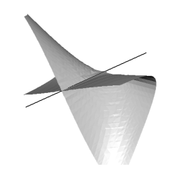
Figure 1. $X_{U}$ on the open set $U_{x_{0}}$

The key feature of this example is that there is a linear syzygy of bidegree $(0,1)$:

$$v\cdot(s^{2}u)-u\cdot(s^{2}v)=0.$$

In Lemmas 3.1 and 4.1 we show that with an appropriate choice of generators for $I_{U}$, any bigraded linear first syzygy has the form above. Existence of a bidegree $(0,1)$ syzygy implies that the pullbacks to ${\mathbb{P}^{1}\times\mathbb{P}^{1}}$ of the two linear forms defining ${\mathbb{P}}(U)$ share a factor. Theorem 8.5 connects this to work of [19].

1.1. Previous work on the $(2,1)$ case

For surfaces in ${\mathbb{P}}^{3}$ of bidegree $(2,1)$, in addition to the classical work of Edge, Salmon and others, more recently Degan [13] studied such surfaces with basepoints and Zube [30], [31] describes the possibilities for the singular locus. In [18], Elkadi-Galligo-Lê give a geometric description of the image and singular locus for a generic $U$ and in [19], Galligo-Lê follow up with an analysis for the nongeneric case. A central part of their analysis is the geometry of a certain dual scroll which we connect to syzygies in §8.

Cox, Dickenstein and Schenck study the bigraded commutative algebra of a three dimensional basepoint free subspace $W\subseteq R_{2,1}$ in [11], showing that there are two numerical types of possible bigraded minimal free resolution of $I_{W}$, determined by how ${\mathbb{P}}(W)\subseteq{\mathbb{P}}(R_{2,1})={\mathbb{P}}^{5}$ meets the image $\Sigma_{2,1}$ of the Segre map ${\mathbb{P}}^{2}\times{\mathbb{P}}^{1}\stackrel{{\scriptstyle\sigma_{2,1}}}{{\longrightarrow}}{\mathbb{P}}^{5}.$ If $W$ is basepoint free, then there are two possibilities: either ${\mathbb{P}}(W)\cap\Sigma_{2,1}$ is a finite set of points, or a smooth conic. The current paper extends the work of [11] to the more complicated setting of a four dimensional space of sections. A key difference is that for a basepoint free subspace $W$ of dimension three, there can never be a linear syzygy on $I_{W}$. As illustrated in the example above, this is not true for the four dimensional case. It turns out that the existence of a linear syzygy provides a very powerful tool for analyzing both the bigraded commutative algebra of $I_{U}$, as well as for determining the implicit equation and singular locus of $X_{U}$. In studying the bigraded commutative algebra of $I_{U}$, we employ a wide range of tools

• Approximation complexes [2], [3], [5], [6], [7].

• Bigraded generic initial ideals [1].

• Geometry of the Segre-Veronese variety [22].

• Fitting ideals and Mapping cones [15].

• Connection between associated primes and Ext modules [16].

• Buchsbaum-Eisenbud exactness criterion [4].

1.2. Approximation complexes

The key tool in connecting the syzygies of $I_{U}$ to the implicit equation for $X_{U}$ is an approximation complex, introduced by Herzog-Simis-Vasconcelos in [23],[24]. We give more details of the construction in §7. The basic idea is as follows: let $R_{I}=R\oplus I_{U}\oplus I_{U}^{2}\oplus\cdots$. Then the graph $\Gamma$ of the map $\phi_{U}$ is equal to $BiProj(R_{I})$ and the embedding of $\Gamma$ in $({\mathbb{P}^{1}\times\mathbb{P}^{1}})\times{\mathbb{P}}(U)$ corresponds to the ring map $S=R[x_{0},\ldots,x_{3}]\stackrel{{\scriptstyle s}}{{\rightarrow}}R_{I}$ given by $x_{i}\mapsto p_{i}$. Let $\beta$ denote the kernel of $s$, so $\beta_{1}$ consists of the syzygies of $I_{U}$ and $S_{I}=Sym_{R}(I)=S/\beta_{1}$. Then

$$\Gamma\subseteq BiProj(S_{I})\subseteq BiProj(S).$$

The works [3], [5], [6], [2] show that if $U$ is basepoint free, then the implicit equation for $X_{U}$ may be extracted from the differentials of a complex $\mathcal{Z}$ associated to the intermediate object $S_{I}$ and in particular the determinant of the complex is a power of the implicit equation. In bidegree $(2,1)$, a result of Botbol [2] shows that the implicit equation may be obtained from a $4\times 4$ minor of $d_{1}$; our work yields an explicit description of the relevant minor.

1.3. Main results

The following two tables describe our classification. Type refers to the graded Betti numbers of the bigraded minimal free resolution for $I_{U}$: we prove there are six numerical types possible. Proposition 6.3 shows that the only possible embedded primes of $I_{U}$ are ${\mathfrak{m}}=\langle s,t,u,v\rangle$ or $P_{i}=\langle l_{i},s,t\rangle$, where $l_{i}$ is a linear form of bidegree $(0,1)$. While Type 5a and 5b have the same bigraded Betti numbers, Proposition 3.2 and Corollary 3.5 show that both the embedded primes and the differentials in the minimal resolution differ. We also connect our classification to the reduced, codimension one singular locus of $X_{U}$. In the table below $T$ denotes a twisted cubic curve, $C$ a smooth plane conic and $L_{i}$ a line.

Type	Lin. Syz.	Emb. Pri.	Sing. Loc.	Example
1	none	${\mathfrak{m}}$	$T$	$\!s^{2}u\!+\!stv,t^{2}u,s^{2}v\!+\!stu,t^{2}v\!+\!stv\!$
2	none	${\mathfrak{m}},P_{1}$	$C\cup L_{1}$	$s^{2}u,t^{2}u,s^{2}v+stu,t^{2}v+stv$
3	1 type $(1,0)$	${\mathfrak{m}}$	$L_{1}$	$s^{2}u+stv,t^{2}u,s^{2}v,t^{2}v+stu$
4	1 type $(1,0)$	${\mathfrak{m}},P_{1}$	$L_{1}$	$stv,t^{2}v,s^{2}v-t^{2}u,s^{2}u$
5a	1 type $(0,1)$	$P_{1},P_{2}$	$L_{1}\cup L_{2}\cup L_{3}$	$s^{2}u,s^{2}v,t^{2}u,t^{2}v+stv$
5b	1 type $(0,1)$	$P_{1}$	$L_{1}\cup L_{2}$	$s^{2}u,s^{2}v,t^{2}u,t^{2}v+stu$
6	2 type $(0,1)$	none	$\emptyset$	$s^{2}u,s^{2}v,t^{2}u,t^{2}v$

Table 1.

The next table gives the possible numerical types for the bigraded minimal free resolutions, where we write $(i,j)$ for the rank one free module $R(i,j)$. We prove more: for Types 3, 4, 5 and 6, we determine all the differentials in the minimal free resolution. One striking feature of Table 1 is that if $I_{U}$ has a linear first syzygy (i.e. of bidegree $(0,1)$ or $(1,0)$), then the codimension one singular locus of $X_{U}$ is either empty or a union of lines. We prove this in Theorem 7.3.

Type	Bigraded Minimal Free Resolution of $I_{U}$ for $U$ basepoint free
1	$0\leftarrow I_{U}\leftarrow(-2,-1)^{4}\longleftarrow\begin{array}[]{c}(-2,-4)\\ \oplus\\ (-3,-2)^{4}\\ \oplus\\ (-4,-1)^{2}\\ \end{array}\longleftarrow\begin{array}[]{c}(-3,-4)^{2}\\ \oplus\\ (-4,-2)^{3}\\ \end{array}\longleftarrow(-4,-4)\leftarrow 0$
2	$0\leftarrow I_{U}\leftarrow(-2,-1)^{4}\longleftarrow\begin{array}[]{c}(-2,-3)\\ \oplus\\ (-3,-2)^{4}\\ \oplus\\ (-4,-1)^{2}\\ \end{array}\longleftarrow\begin{array}[]{c}(-3,-3)^{2}\\ \oplus\\ (-4,-2)^{3}\\ \end{array}\longleftarrow(-4,-3)\leftarrow 0$
3	$0\leftarrow I_{U}\leftarrow(-2,-1)^{4}\longleftarrow\begin{array}[]{c}(-2,-4)\\ \oplus\\ (-3,-1)\\ \oplus\\ (-3,-2)^{2}\\ \oplus\\ (-3,-3)\\ \oplus\\ (-4,-2)\\ \oplus\\ (-5,-1)\\ \end{array}\longleftarrow\begin{array}[]{c}(-3,-4)^{2}\\ \oplus\\ (-4,-3)^{2}\\ \oplus\\ (-5,-2)^{2}\\ \end{array}\longleftarrow\begin{array}[]{c}(-4,-4)\\ \oplus\\ (-5,-3)\\ \end{array}\leftarrow 0$
4	$0\leftarrow I_{U}\leftarrow(-2,-1)^{4}\longleftarrow\begin{array}[]{c}(-2,-3)\\ \oplus\\ (-3,-1)\\ \oplus\\ (-3,-2)^{2}\\ \oplus\\ (-4,-2)\\ \oplus\\ (-5,-1)\\ \end{array}\longleftarrow\begin{array}[]{c}(-3,-3)\\ \oplus\\ (-4,-3)\\ \oplus\\ (-5,-2)^{2}\\ \end{array}\longleftarrow(-5,-3)\leftarrow 0$
5	​​​​​​​​​​​​​​​​​​​​​​​​​​​​​​​​​​​​​​​​​$0\leftarrow I_{U}\leftarrow(-2,-1)^{4}\longleftarrow\begin{array}[]{c}(-2,-2)\\ \oplus\\ (-3,-2)^{2}\\ \oplus\\ (-4,-1)^{2}\\ \end{array}\longleftarrow(-4,-2)^{2}\leftarrow 0$
6	​​​​​​​​​​​​​​​​​​​​​​​​​​​​​​​​​​​​​​​​​​​​$0\leftarrow I_{U}\leftarrow(-2,-1)^{4}\longleftarrow\begin{array}[]{c}(-2,-2)^{2}\\ \oplus\\ (-4,-1)^{2}\\ \end{array}\longleftarrow(-4,-2)\leftarrow 0$

Table 2.

2. Geometry and the Segre-Veronese variety

Consider the composite maps

(2.1)

The first horizontal map is $\nu_{2}\times id$, where $\nu_{2}$ is the 2-uple Veronese embedding and the second horizontal map is the Segre map $\sigma_{2,1}:\mathbb{P}^{2}\times\mathbb{P}^{1}\rightarrow\mathbb{P}^{5}$. The image of $\sigma_{2,1}$ is a smooth irreducible nondegenerate cubic threefold $\Sigma_{2,1}$. Any ${\mathbb{P}}^{2}\subseteq\Sigma_{2,1}$ is a fiber over a point of the ${\mathbb{P}}^{1}$ factor and any ${\mathbb{P}}^{1}\subseteq\Sigma_{2,1}$ is contained in the image of a fiber over ${\mathbb{P}}^{2}$ or ${\mathbb{P}}^{1}$. For this see Chapter 2 of [21], which also points out that the Segre and Veronese maps have coordinate free descriptions

$$\begin{array}[]{ccc}\mathbb{P}(A)&\stackrel{{\scriptstyle\nu_{d}}}{{\longrightarrow}}&\mathbb{P}(Sym^{d}A)\\ \mathbb{P}(A)\times\mathbb{P}(B)&\stackrel{{\scriptstyle\sigma}}{{\longrightarrow}}&\mathbb{P}(A\otimes B)\end{array}$$

By dualizing we may interpret the image of $\nu_{d}$ as the variety of $d^{th}$ powers of linear forms on $A$ and the image of $\sigma$ as the variety of products of linear forms. The composition $\tau=\sigma_{2,1}\circ(\nu_{2}\times id)$ is a Segre-Veronese map, with image consisting of polynomials which factor as $l_{1}(s,t)^{2}\cdot l_{2}(u,v)$. Note that $\Sigma_{2,1}$ is also the locus of polynomials in $R_{2,1}$ which factor as $q(s,t)\cdot l(u,v)$, with $q\in R_{2,0}$ and $l\in R_{0,1}$. Since $q\in R_{2,0}$ factors as $l_{1}\cdot l_{2}$, this means $\Sigma_{2,1}$ is the locus of polynomials in $R_{2,1}$ which factor completely as products of linear forms. As in the introduction,

$$U\subseteq H^{0}({\mathcal{O}_{\mathbb{P}^{1}\times\mathbb{P}^{1}}}(2,1))=V={\mathrm{Span}}\{s^{2}u,stu,t^{2}u,s^{2}v,stv,t^{2}v\}.$$

The ideal of $\Sigma_{2,1}$ is defined by the two by two minors of

$$\left[\begin{matrix}x_{0}&x_{1}&x_{2}\\ x_{3}&x_{4}&x_{5}\end{matrix}\right].$$

It will also be useful to understand the intersection of ${\mathbb{P}}(U)$ with the locus of polynomials in $V$ which factor as the product of a form $q=a_{0}su+a_{1}sv+a_{2}tu+a_{3}tv$ of bidegree $(1,1)$ and $l=b_{0}s+b_{1}t$ of bidegree $(1,0)$. This is the image of the map

$${\mathbb{P}}(H^{0}({\mathcal{O}_{\mathbb{P}^{1}\times\mathbb{P}^{1}}}(1,1)))\times{\mathbb{P}}(H^{0}({\mathcal{O}_{\mathbb{P}^{1}\times\mathbb{P}^{1}}}(1,0)))={\mathbb{P}}^{3}\times{\mathbb{P}}^{1}\longrightarrow{\mathbb{P}}^{5},$$

$(a_{0}:a_{1}:a_{2}:a_{3})\times(b_{0}:b_{1})\mapsto(a_{0}b_{0}:a_{0}b_{1}+a_{2}b_{0}:a_{2}b_{1}:a_{1}b_{0}:a_{1}b_{1}+a_{3}b_{0}:a_{3}b_{1})$, which is a quartic hypersurface

$$Q={\bf V}({x}_{2}^{2}{x}_{3}^{2}-{x}_{1}{x}_{2}{x}_{3}{x}_{4}+{x}_{0}{x}_{2}{x}_{4}^{2}+{x}_{1}^{2}{x}_{3}{x}_{5}-2{x}_{0}{x}_{2}{x}_{3}{x}_{5}-{x}_{0}{x}_{1}{x}_{4}{x}_{5}+{x}_{0}^{2}{x}_{5}^{2}).$$

As Table 1 shows, the key to classifying the minimal free resolutions is understanding the linear syzygies. In §3, we show that if $I_{U}$ has a first syzygy of bidegree $(0,1)$, then after a change of coordinates, $I_{U}=\langle pu,pv,p_{2},p_{3}\rangle$ and if $I_{U}$ has a first syzygy of bidegree $(1,0)$, then $I_{U}=\langle ps,pt,p_{2},p_{3}\rangle$.

Proposition 2.1.

If $U$ is basepoint free, then the ideal $I_{U}$

1. has a unique linear syzygy of bidegree $(0,1)$ iff $F\subseteq{\mathbb{P}}(U)\cap\Sigma_{2,1}$, where $F$ is a ${\mathbb{P}}^{1}$ fiber of $\Sigma_{2,1}$.

2. has a pair of linear syzygies of bidegree $(0,1)$ iff ${\mathbb{P}}(U)\cap\Sigma_{2,1}=\Sigma_{1,1}$.

3. has a unique linear syzygy of bidegree $(1,0)$ iff $F\subseteq{\mathbb{P}}(U)\cap Q$, where $F$ is a ${\mathbb{P}}^{1}$ fiber of $Q$.

Proof.

The ideal $I_{U}$ has a unique linear syzygy of bidegree $(0,1)$ iff $qu,qv\in I_{U}$, with $q\in R_{2,0}$ iff $q\cdot l(u,v)\in I_{U}$ for all $l(u,v)\in R_{0,1}$ iff ${\mathbb{P}}(U)\cap\Sigma_{2,1}$ contains the ${\mathbb{P}}^{1}$ fiber over the point $q\in{\mathbb{P}}(R_{2,0})$.

For the second item, the reasoning above implies that ${\mathbb{P}}(U)\cap\Sigma_{2,1}$ contains two ${\mathbb{P}}^{1}$ fibers, over points $q_{1},q_{2}\in{\mathbb{P}}(R_{2,0})$. But then $I_{U}$ also contains the line in ${\mathbb{P}}(R_{2,0})$ connecting $q_{1}$ and $q_{2}$, as well as the ${\mathbb{P}}^{1}$ lying over any point on the line, yielding a ${\mathbb{P}}^{1}\times{\mathbb{P}}^{1}$.

For the third part, a linear syzygy of bidegree $(1,0)$ means that $qs,qt\in I_{U}$, with $q\in R_{1,1}$ iff $q\cdot l(s,t)\in I_{U}$ for all $l(s,t)\in R_{1,0}$ iff ${\mathbb{P}}(U)\cap Q$ contains the ${\mathbb{P}}^{1}$ fiber over the point $q\in{\mathbb{P}}(R_{1,1})$. ∎

In Theorem 4.6, we show that Proposition 2.1 describes all possible linear syzygies.

3. First syzygies of bidegree $(0,1)$

Our main result in this section is a complete description of the minimal free resolution when $I_{U}$ has a first syzygy of bidegree $(0,1)$. As a consequence, if $I_{U}$ has a unique first syzygy of bidegree $(0,1)$, then the minimal free resolution has numerical Type 5 and if there are two linear first syzygies of bidegree $(0,1)$, the minimal free resolution has numerical Type 6. We begin with a simple observation

Lemma 3.1.

If $I_{U}$ has a linear first syzygy of bidegree $(0,1)$, then

$$I_{U}=\langle pu,pv,p_{2},p_{3}\rangle,$$

where $p$ is homogeneous of bidegree $(2,0)$.

Proof.

Rewrite the syzygy

$$\sum\limits_{i=0}^{3}(a_{i}u+b_{i}v)p_{i}=0=u\cdot\sum\limits_{i=0}^{3}a_{i}p_{i}+v\cdot\sum\limits_{i=0}^{3}b_{i}p_{i},$$

and let $g_{0}=\sum\limits_{i=0}^{3}a_{i}p_{i}$, $g_{1}=\sum\limits_{i=0}^{3}b_{i}p_{i}$. The relation above implies that $(g_{0},g_{1})$ is a syzygy on $(u,v)$. Since the syzygy module of $(u,v)$ is generated by the Koszul syzygy, this means

$$\left[\!\begin{array}[]{c}g_{0}\\ g_{1}\end{array}\!\right]=p\cdot\left[\!\begin{array}[]{c}-v\\ u\end{array}\!\right]$$

∎

A similar argument applies if $I_{U}$ has a first syzygy of degree $(1,0)$. Lemma 3.1 has surprisingly strong consequences:

Proposition 3.2.

If $U$ is basepoint free and $I_{U}$ has a unique linear first syzygy of bidegree $(0,1)$, then there is a complex of free $R$ modules

$$\mathcal{F}_{1}\mbox{ : }0\longrightarrow F_{3}\stackrel{{\scriptstyle\phi_{3}}}{{\longrightarrow}}F_{2}\stackrel{{\scriptstyle\phi_{2}}}{{\longrightarrow}}F_{1}\stackrel{{\scriptstyle\phi_{1}}}{{\longrightarrow}}I_{U}\longrightarrow 0,$$

where $\phi_{1}=\left[\!\begin{array}[]{cccc}p_{0}&p_{1}&p_{2}&p_{3}\end{array}\!\right]$, with ranks and shifts matching Type 5 in Table 2. Explicit formulas appear in the proof below. The differentials $\phi_{i}$ depend on whether $p=L_{1}(s,t)L_{2}(s,t)$ of Lemma 3.1 has $L_{1}=L_{2}$.

Proof.

Since $I_{U}$ has a syzygy of bidegree $(0,1)$, by Lemma 3.1, $I_{U}=\langle pu,pv,p_{2},p_{3}\rangle$.
Case 1: Suppose $p=l(s,t)^{2}$, then after a change of coordinates, $p=s^{2}$, so $p_{0}=s^{2}u$ and $p_{1}=s^{2}v$. Eliminating terms from $p_{2}$ and $p_{3}$, we may assume

$$\begin{array}[]{ccc}p_{2}&=&stl_{1}(u,v)+t^{2}l_{2}(u,v)=t(sl_{1}(u,v)+tl_{2}(u,v))\\ p_{3}&=&stl_{3}(u,v)+t^{2}l_{4}(u,v)=t(sl_{3}(u,v)+tl_{4}(u,v)).\end{array}$$

Let $l_{i}(u,v)=a_{i}u+b_{i}v$ and define

$$A(u,v)=\left[\!\begin{array}[]{cc}l_{1}&l_{2}\\ l_{3}&l_{4}\end{array}\!\right].$$

Note that det $A(u,v)=q(u,v)\neq 0$. The rows cannot be dependent, since $U$ spans a four dimensional subspace. If the columns are dependent, then $\{p_{2},p_{3}\}=\{tl_{1}(s+kt),tl_{2}(s+kt)\}$, yielding another syzygy of bidegree $(0,1)$, contradicting our hypothesis. In the proof of Corollary 3.4, we show the hypothesis that $U$ is basepoint free implies that $A(u,v)$ is a $1$-generic matrix, which means that $A(u,v)$ cannot be made to have a zero entry using row and column operations. We obtain a first syzygy of bidegree $(2,0)$ as follows:

$$\begin{array}[]{ccl}s^{2}p_{2}&=&s^{3}tl_{1}+s^{2}t^{2}l_{2}\\ &=&(a_{1}st+a_{2}t^{2})s^{2}u+(b_{1}st+b_{2}t^{2})s^{2}v\\ &=&(a_{1}st+a_{2}t^{2})p_{0}+(b_{1}st+b_{2}t^{2})p_{1}\\ \end{array}$$

A similar relation holds for $stp_{3}$, yielding two first syzygies of bidegree $(2,0)$. We next consider first syzygies of bidegree $(1,1)$. There is an obvious syzygy on $p_{2},p_{3}$ given by

$$\begin{array}[]{ccccc}(sl_{1}(u,v)+tl_{2}(u,v))p_{3}&=&(sl_{3}(u,v)+tl_{4}(u,v))p_{2}\end{array}$$

Since ${\mathrm{det}}A(s,t)=q(u,v)\neq 0$, from

$$\begin{array}[]{ccc}t^{2}q&=&l_{3}p_{2}-l_{1}p_{3}\\ stq&=&l_{4}p_{2}-l_{2}p_{3}\end{array}$$

and the fact that $q(u,v)=L_{1}(u,v)L_{2}(u,v)$ with $L_{i}(u,v)=\alpha_{i}u+\beta_{i}v$, so we obtain a pair of relations of bidegree $(1,1)$:

$$\begin{array}[]{ccccc}sl_{4}p_{2}-sl_{2}p_{3}&=&s^{2}tL_{1}L_{2}&=&(\alpha_{1}tL_{2})s^{2}u+(\beta_{1}tL_{2})s^{2}v.\end{array}$$

Case 2: $p=l(s,t)\cdot l^{\prime}(s,t)$ with $l,l^{\prime}$ independent linear forms. Then after a change of coordinates, $p=st$, so $p_{0}=stu$ and $p_{1}=stv$. Eliminating terms from $p_{2}$ and $p_{3}$, we may assume

$$\begin{array}[]{ccc}p_{2}&=&s^{2}l_{1}(u,v)+t^{2}l_{2}(u,v)\\ p_{3}&=&s^{2}l_{3}(u,v)+t^{2}l_{4}(u,v).\end{array}$$

Let $l_{i}(u,v)=a_{i}u+b_{i}v$. We obtain a first syzygy of bidegree $(2,0)$ as follows:

$$\begin{array}[]{ccc}stp_{2}&=&\!\!\!\!\!\!\!\!\!\!\!\!\!\!\!\!\!\!\!\!\!\!\!\!\!\!\!\!\!\!\!\!\!\!\!\!\!\!\!\!\!\!\!\!\!\!\!\!\!\!\!\!\!\!\!\!s^{3}tl_{1}+st^{3}l_{2}\\ &=&\!\!\!\!\!\!\!\!\!\!\!\!\!\!\!\!\!\!\!\!\!\!\!\!\!\!\!\!\!\!\!\!\!\!\!\!\!\!\!\!\!\!s^{2}(stl_{1})+t^{2}(stl_{2})\\ &=&(a_{1}s^{2}+a_{2}t^{2})stu+(b_{1}s^{2}+b_{2}t^{2})stv\end{array}$$

A similar relation holds for $stp_{3}$, yielding two first syzygies of bidegree $(2,0)$. We next consider first syzygies of bidegree $(1,1)$. Since $q(u,v)\neq 0$, from

$$\begin{array}[]{ccc}t^{2}q&=&l_{3}p_{2}-l_{1}p_{3}\\ s^{2}q&=&l_{4}p_{2}-l_{2}p_{3}\end{array}$$

and the fact that $q(u,v)=L_{1}(u,v)L_{2}(u,v)$ with $L_{i}(u,v)=\alpha_{i}u+\beta_{i}v$, we have relations

$$\begin{array}[]{ccccc}sl_{3}p_{2}-sl_{1}p_{3}&=&st^{2}L_{1}L_{2}&=&(\alpha_{1}tL_{2})stu+(\beta_{1}tL_{2})stv\\ tl_{4}p_{2}-tl_{2}p_{3}&=&ts^{2}L_{1}L_{2}&=&(\alpha_{1}sL_{2})stu+(\beta_{1}sL_{2})stv,\end{array}$$

which yield a pair of first syzygies of bidegree $(1,1)$. Putting everything together, we now have candidates for the differential $\phi_{2}$ in both cases. Computations exactly like those above yield similar candidates for $\phi_{3}$ in the two cases. In Case 1, we have

$$\phi_{2}=\left[\!\begin{array}[]{ccccc}v&\alpha_{1}tL_{2}&0&a_{1}st+a_{2}t^{2}&a_{3}st+a_{4}t^{2}\\ -u&\beta_{1}tL_{2}&0&b_{1}st+b_{2}t^{2}&b_{3}st+b_{4}t^{2}\\ 0&-sl_{4}&sl_{3}+tl_{4}&-s^{2}&0\\ 0&sl_{2}&-sl_{1}-tl_{2}&0&-s^{2}\end{array}\!\right],\mbox{ }\phi_{3}=\left[\!\begin{array}[]{cc}\gamma&\delta\\ s&t\\ 0&s\\ -l_{4}&-l_{3}\\ l_{2}&l_{1}\end{array}\!\right],$$

where

$$\begin{array}[]{lll}\delta&=&-\alpha_{1}\beta_{2}t^{2}+(a_{1}st+a_{2}t^{2})b_{3}-(a_{3}st+a_{4}t^{2})b_{1}\\ \gamma&=&-\alpha_{1}\beta_{2}st+(a_{1}st+a_{2}t^{2})b_{4}-(a_{3}st+a_{4}t^{2})b_{2}\end{array}$$

For $I_{U}$ as in Case 2, let

$$\phi_{2}=\left[\!\begin{array}[]{ccccc}v&\alpha_{1}tL_{2}&\alpha_{1}sL_{2}&a_{1}s^{2}+a_{2}t^{2}&a_{3}s^{2}+a_{4}t^{2}\\ -u&\beta_{1}tL_{2}&\beta_{1}sL_{2}&b_{1}s^{2}+b_{2}t^{2}&b_{3}s^{2}+b_{4}t^{2}\\ 0&-sl_{3}&-tl_{4}&-st&0\\ 0&sl_{1}&tl_{2}&0&-st\end{array}\!\right],\mbox{ }\phi_{3}=\left[\!\begin{array}[]{cc}\gamma&\delta\\ 0&t\\ s&0\\ -l_{4}&-l_{3}\\ l_{2}&l_{1}\end{array}\!\right],$$

where

$$\begin{array}[]{ccc}\gamma&=&(-\alpha_{1}\beta_{2}+a_{1}b_{4}-a_{3}b_{2})s^{2}+(a_{2}b_{4}-a_{4}b_{2})t^{2}\\ \delta&=&(a_{1}b_{3}-a_{3}b_{1})s^{2}+(-\alpha_{1}\beta_{2}+a_{2}b_{3}-a_{4}b_{1})t^{2}\end{array}$$

We have already shown that ${\mathrm{im}}(\phi_{2})\subseteq\ker(\phi_{1})$, and an easy check shows that ${\mathrm{im}}(\phi_{3})\subseteq\ker(\phi_{2})$, yielding a complex of free modules of numerical Type 5. ∎

To prove that the complex above is actually exact, we use the following result of Buchsbaum and Eisenbud [4]: a complex of free modules

$$\mathcal{F}:\cdots\stackrel{{\scriptstyle\phi_{i+1}}}{{\longrightarrow}}F_{i}\stackrel{{\scriptstyle\phi_{i}}}{{\longrightarrow}}F_{i-1}\stackrel{{\scriptstyle\phi_{i-1}}}{{\longrightarrow}}\cdots F_{1}\stackrel{{\scriptstyle\phi_{1}}}{{\longrightarrow}}F_{0},$$

is exact iff

1. ${\mathrm{rank}}(\phi_{i+1})+{\mathrm{rank}}(\phi_{i})={\mathrm{rank}}(F_{i})$.

2. $0pt(I_{{\mathrm{rank}}(\phi_{i})}(\phi_{i}))\geq i$.

Theorem 3.3.

The complexes appearing in Proposition 3.2 are exact.

Proof.

Put $F_{0}=R$. An easy check shows that ${\mathrm{rank}}(\phi_{i+1})+{\mathrm{rank}}(\phi_{i})={\mathrm{rank}}(F_{i})$, so what remains is to show that $0pt(I_{2}(\phi_{3}))\geq 3$ and $0pt(I_{3}(\phi_{2}))\geq 2$. The fact that $s\nmid\gamma$ will be useful: to see this, note that both Case 1 and Case 2, $s\mid\gamma$ iff $a_{2}b_{4}-b_{2}a_{4}=0$, which implies $l_{2}$ and $l_{4}$ differ only by a scalar, contradicting the assumption that $U$ is basepoint free.
Case 1: We have $us^{4},vs^{4}\in I_{3}(\phi_{2})$. Consider the minor

$$\lambda=t^{2}L_{2}(sl_{1}+tl_{2})\left((\alpha_{1}b_{1}-\beta_{1}a_{1})s+(\alpha_{1}b_{2}-\beta_{1}a_{2})t\right)$$

obtained from the submatrix

$$\left[\begin{array}[]{ccc}\alpha_{1}tL_{2}&0&a_{1}st+a_{2}t^{2}\\ \beta_{1}tL_{2}&0&b_{1}st+b_{2}t^{2}\\ sl_{2}&-sl_{1}-tl_{2}&0\end{array}\!\right]$$

Note that $s$ does not divide $\lambda$, for if $s|\lambda$ then either $l_{2}=0$ or $\alpha_{1}b_{2}-\beta_{1}a_{2}=0$. But none of the $l_{i}$ can be zero because of the basepoint free assumption (see the proof of Corollary 3.4) and if $\alpha_{1}b_{2}-\beta_{1}a_{2}=0$, then $L_{1}$ and $l_{2}$ are the same up to a scalar multiple. Hence, since $l_{1}l_{4}-l_{2}l_{3}=L_{1}L_{2}$, we obtain $l_{1}$ is equal to a scalar multiple of $l_{2}$ or $l_{3}$, which again violates the basepoint free assumption. To conclude, note that $u$ and $v$ can not divide $\lambda$ at the same time, therefore, $\lambda$ and one of the $us^{4}$ and $vs^{4}$ form a regular sequence in $I_{3}(\phi_{2})$, showing that depth of $I_{3}(\phi_{2})$ is at least $2$.
To show that $0pt(I_{2}(\phi_{3}))\geq 3$, note that

$$I_{2}(\phi_{3})=\langle sl_{2},sl_{4},tl_{4}-sl_{3},tl_{2}-sl_{1},t\gamma-s\delta,s\gamma,s^{2},q(u,v)\rangle$$

Since $l_{2},l_{4}$ are independent, $\langle sl_{2},sl_{4}\rangle=\langle su,sv\rangle$ and using these we can reduce $tl_{4}-sl_{3},tl_{2}-sl_{1}$ to $tu,tv$. Since $s\nmid\gamma$, modulo $s^{2}$, $s\gamma$ reduces to $st^{2}$. Similarly, $t\gamma-s\delta$ reduces to $t^{3}$, so that in fact

$$I_{2}(\phi_{3})=\langle su,sv,tu,tv,s^{2},st^{2},t^{3},q(u,v)\rangle,$$

and $\{s^{2},t^{3},q(u,v)\}$ is a regular sequence of length three.
Case 2: We have $us^{2}t^{2},vs^{2}t^{2}\in I_{3}(\phi_{2})$. Consider the minor

$$\lambda=L_{2}(s^{2}l_{1}-t^{2}l_{2})\left((\alpha_{1}b_{1}-\beta_{1}a_{1})s^{2}+(\alpha_{1}b_{2}-\beta_{1}a_{2})t^{2}\right)$$

arising from the submatrix

$$\left[\begin{array}[]{ccc}\alpha_{1}tL_{2}&\alpha_{1}sL_{2}&a_{1}s^{2}+a_{2}t^{2}\\ \beta_{1}tL_{2}&\beta_{1}sL_{2}&b_{1}s^{2}+b_{2}t^{2}\\ sl_{1}&tl_{2}&0\end{array}\!\right]$$

Note that $s$ and $t$ do not divide $\lambda$, for if $s|\lambda$ then either $l_{2}=0$ or $\alpha_{1}b_{2}-\beta_{1}a_{2}=0$. But none of the $l_{i}$ can be zero because of the basepoint free assumption (see the proof of Corollary 3.4) and if $\alpha_{1}b_{2}-\beta_{1}a_{2}=0$, then $L_{1}$ and $l_{2}$ are the same up to a scalar multiple. Hence, since $l_{1}l_{4}-l_{2}l_{3}=L_{1}L_{2}$, we obtain $l_{1}$ is equal to a scalar multiple of $l_{2}$ or $l_{3}$, contradicting basepoint freeness. Furthermore, $u$ and $v$ cannot divide $\lambda$ at the same time, so $\lambda$ and one of the $us^{2}t^{2}$ and $vs^{2}t^{2}$ form a regular sequence in $I_{3}(\phi_{2})$. To show that $0pt(I_{2}(\phi_{3}))\geq 3$, note that

$$I_{2}(\phi_{3})=\langle su,sv,tu,tv,st,t\gamma,s\delta,q(u,v)\rangle,$$

where we have replaced $sl_{i},tl_{j}$ as in Case 1. If $t\mid\delta$, then $a_{1}b_{3}-b_{1}a_{3}=0$, which would mean $l_{1}=kl_{3}$ and contradict that $U$ is basepoint free. Since $s\nmid\gamma$ and $t\nmid\delta$, $\{t\gamma,s\delta,q(u,v)\}$ is regular unless $\delta$, $\gamma$ share a common factor $\eta=(as+bt)$. Multiplying out and comparing coefficients shows that this forces $\gamma$ and $\delta$ to agree up to scalar. Combining this with the fact that $t\nmid\delta$, $s\nmid\delta$, we find that $\delta=as^{2}+bst+ct^{2}$ with $a\neq 0\neq c$. Reducing $s\delta$ and $t\delta$ by $st$ then implies that $t^{3},s^{3}\in I_{2}(\phi_{3})$. ∎

Corollary 3.4.

If $U$ is basepoint free, then $I_{U}$ cannot have first syzygies of both bidegree $(0,1)$ and bidegree $(1,0)$.

Proof.

Suppose there is a first syzygy of bidegree $(0,1)$ and proceed as in the proof of Proposition 3.2. In the setting of Case 1,

$$I_{U}=\langle stu,stv,s^{2}l_{1}(u,v)+t^{2}l_{2}(u,v),s^{2}l_{3}(u,v)+t^{2}l_{4}(u,v)\rangle.$$

If there is also a linear syzygy of bidegree $(1,0)$, expanding out $\sum(a_{i}s+b_{i}t)p_{i}$ shows that the coefficient of $s^{3}$ is $a_{3}l_{1}+a_{4}l_{3}$, and the coefficient of $t^{3}$ is $b_{3}l_{2}+b_{4}l_{4}$. Since $\sum(a_{i}s+b_{i}t)p_{i}=0$, both coefficients must vanish. In the proof of Proposition 3.2 we showed ${\mathrm{det}}A(u,v)=q(u,v)\neq 0$. In fact, more is true: if any of the $l_{i}$ is zero, then $U$ is not basepoint free. For example, if $l_{1}=0$, then $\langle t,l_{3}\rangle$ is a minimal associated prime of $I_{U}$. Since $a_{3}l_{1}+a_{4}l_{3}=0$ iff $a_{3}=a_{4}=0$ or $l_{1}$ is a scalar multiple of $l_{3}$ and the latter situation implies that $U$ is not basepoint free, we must have $a_{3}=a_{4}=0$. Reasoning similarly for $b_{3}l_{2}+b_{4}l_{4}$ shows that $a_{3}=a_{4}=b_{3}=b_{4}=0$. This implies the linear syzygy of bidegree $(1,0)$ can only involve $stu,stv$, which is impossible. This proves the result in Case 1 and similar reasoning works for Case 2. ∎

Corollary 3.5.

If $I_{U}$ has a unique linear first syzygy of bidegree $(0,1)$, then $I_{U}$ has either one or two embedded prime ideals of the form $\langle s,t,L_{i}(u,v)\rangle$. If $q(u,v)={\mathrm{det}}~{}A(u,v)=L_{1}(u,v)L_{2}(u,v)$ for $A(u,v)$ as in Theorem 3.3, then:

1. If $L_{1}=L_{2}$, then the only embedded prime of $I_{U}$ is $\langle s,t,L_{1}\rangle$.

2. If $L_{1}\neq L_{2}$, then $I_{U}$ has two embedded primes $\langle s,t,L_{1}\rangle$ and $\langle s,t,L_{2}\rangle$.

Proof.

In [16], Eisenbud, Huneke and Vasconcelos show that a prime $P$ of codimension $c$ is associated to $R/I$ iff it is associated to $Ext^{c}(R/I,R)$. If $I_{U}$ has a unique linear syzygy, then the free resolution is given by Proposition 3.2, and $Ext^{3}(R/I_{U},R)={\mathrm{coker}}(\phi_{3}^{t})$. By Proposition 20.6 of [15], if $\phi$ is a presentation matrix for a module $M$, then the radicals of $ann(M)$ and $I_{{\mathrm{rank}}(\phi)}(\phi)$ are equal. Thus, if $I_{U}$ has a Type 5 resolution, the codimension three associated primes are the codimension three associated primes of $I_{2}(\phi_{3})$. The proof of Theorem 3.3 shows that in Case 1,

$$\begin{array}[]{cccc}I_{2}(\phi_{3})&=&\!\!\!\!\!\!\!\!\!\!\!\!\!\!\!\langle su,sv,tu,tv,s^{2},st^{2},t^{3},q(u,v)\rangle&\\ &=&\!\!\!\!\!\!\!\!\!\!\!\!\!\!\!\!\!\!\!\!\!\!\!\!\!\!\!\!\!\langle s^{2},st^{2},t^{3},u,v\rangle\cap\langle s,t,L_{1}^{2}\rangle&\mbox{ if }L_{1}=L_{2}\\ &=&\langle s^{2},st^{2},t^{3},u,v\rangle\cap\langle s,t,L_{1}\rangle\cap\langle s,t,L_{2}\rangle&\mbox{ if }L_{1}\neq L_{2}.\\ \end{array}$$

The embedded prime associated to $\langle s,t,u,v\rangle$ is not an issue, since we are only interested in the codimension three associated primes. The proof for Case 2 works in the same way. ∎

Next, we tackle the case where the syzygy of bidegree $(0,1)$ is not unique.

Proposition 3.6.

If $U$ is basepoint free, then the following are equivalent

1. The ideal $I_{U}$ has two linear first syzygies of bidegree $(0,1)$.

2. The primary decomposition of $I_{U}$ is

   $$I_{U}=\langle u,v\rangle\cap\langle q_{1},q_{2}\rangle,$$

   where $\sqrt{\langle q_{1},q_{2}\rangle}=\langle s,t\rangle$ and $q_{i}$ are of bidegree $(2,0)$.

3. The minimal free resolution of $I_{U}$ is of numerical Type 6.

4. $X_{U}\simeq\Sigma_{1,1}$.

Proof.

By Lemma 3.1, since $I_{U}$ has a linear syzygy of bidegree $(0,1)$,

$$I_{U}=\langle q_{1}u,q_{1}v,p_{2},p_{3}\rangle.$$

Proceed as in the proof of Proposition 3.2. In Case 1, the assumption that $q_{1}=st$ means that $p_{2},p_{3}$ can be reduced to have no terms involving $stu$ and $stv$, hence there cannot be a syzygy of bidegree $(0,1)$ involving $p_{i}$ and $q_{1}u,q_{1}v$. Therefore the second first syzygy of bidegree $(0,1)$ involves only $p_{2}$ and $p_{3}$ and the reasoning in the proof of Lemma 3.1 implies that $\langle p_{2},p_{3}\rangle=\langle q_{2}u,q_{2}v\rangle$. Thus, we have the primary decomposition

$$I_{U}=\langle q_{1},q_{2}\rangle\cap\langle u,v\rangle,$$

with $q_{1},q_{2}$ of bidegree $(2,0)$. Since $U$ is basepoint free, $\sqrt{q_{1},q_{2}}=\langle s,t\rangle$, so $q_{1}$ and $q_{2}$ are a regular sequence in $k[s,t]$. Similar reasoning applies in the situation of Case 2. That the minimal free resolution is of numerical Type 6 follows from the primary decomposition above, which determines the differentials in the minimal free resolution:

$$I_{U}\longleftarrow(-2,-1)^{4}\xleftarrow{\left[\!\begin{array}[]{cccc}v&0&q_{2}&0\\ -u&0&0&q_{2}\\ 0&v&-q_{1}&0\\ 0&-u&0&-q_{1}\end{array}\!\right]}\begin{array}[]{c}(-2,-2)^{2}\\ \oplus\\ (-4,-1)^{2}\end{array}\!\xleftarrow{\left[\!\begin{array}[]{c}q_{2}\\ -q_{1}\\ -v\\ u\end{array}\!\right]}(-4,-2).$$

The last assertion follows since

$${\mathrm{det}}\left[\!\begin{array}[]{cc}uq_{1}&uq_{2}\\ vq_{1}&vq_{2}\end{array}\!\right]=0.$$

Hence, the image of $\phi_{U}$ is contained in ${\bf V}(xy-zw)=\Sigma_{1,1}$. After a change of coordinates, $q_{1}=s^{2}+ast$ and $q_{2}=t^{2}+bst$, with $0\neq a\neq b\neq 0$. Therefore on the open set $U_{s,u}\subseteq{\mathbb{P}^{1}\times\mathbb{P}^{1}}$ the map is defined by

$$(at+1,(at+1)v,t^{2}+bt,(t^{2}+bt)u),$$

so the image is a surface. Finally, if $X_{U}=\Sigma_{1,1}$, then with a suitable choice of basis for $U$, $p_{0}p_{3}-p_{1}p_{2}=0$, hence $p_{0}|p_{1}p_{2}$ and $p_{3}|p_{1}p_{2}$. Since $U$ is four dimensional, this means we must have $p_{0}=\alpha\beta$, $p_{1}=\alpha\gamma$, $p_{2}=\beta\delta$. Without loss of generality, suppose $\beta$ is quadratic, so there is a linear first syzygy $\delta p_{0}-\alpha p_{2}=0$. Arguing similarly for $p_{3}$, we find that there are two independent linear first syzygies. Lemma 4.4 of the next section shows that if $U$ is basepoint free, then there can be at most one first syzygy of bidegree $(1,0)$, so by Corollary 3.4, $I_{U}$ must have two first syzygies of bidegree $(0,1)$. ∎

4. First syzygies of bidegree $(1,0)$

Recall that there is an analogue of Lemma 3.1 for syzygies of bidegree $(1,0)$:

Lemma 4.1.

If $I_{U}$ has a linear syzygy of bidegree $(1,0)$, then

$$I_{U}=\langle ps,pt,p_{2},p_{3}\rangle,$$

where $p$ is homogeneous of bidegree $(1,1)$.

Lemma 4.1 has strong consequences as well: we will prove that

Proposition 4.2.

If $U$ is basepoint free and $I_{U}=\langle ps,pt,p_{2},p_{3}\rangle$, then

1. $I_{U}$ has numerical Type 4 if and only if $p$ is decomposable.

2. $I_{U}$ has numerical Type 3 if and only if $p$ is indecomposable.

We begin with some preliminary lemmas:

Lemma 4.3.

If $I_{U}$ has a first syzygy of bidegree $(1,0)$, then $I_{U}$ has two minimal syzygies of bidegree $(1,1)$ and if $p$ in Lemma 4.1 factors, then $I_{U}$ also has a minimal first syzygy of bidegree $(0,2)$.

Proof.

First assume $p$ is an irreducible bidegree $(1,1)$ form, then $p=a_{0}su+a_{1}sv+a_{2}tu+a_{3}tv$, with $a_{0}a_{3}-a_{1}a_{2}\neq 0$. We may assume $a_{0}\neq 0$ and scale so it is one. Then

$$\begin{array}[]{ccc}sp&=&s^{2}u+a_{1}s^{2}v+a_{2}stu+a_{3}stv\\ tp&=&stu+a_{1}stv+a_{2}t^{2}u+a_{3}t^{2}v\\ p_{2}&=&b_{0}t^{2}u+b_{1}s^{2}v+b_{2}stv+b_{3}t^{2}v\\ p_{3}&=&c_{0}t^{2}u+c_{1}s^{2}v+c_{2}stv+c_{3}t^{2}v\\ \end{array}$$

Here we have used $tp$ and $sp$ to remove all the terms involving $s^{2}u$ and $stu$ from $p_{2}$ and $p_{3}$. A simple but tedious calculation then shows that

$$\begin{array}[]{ccc}p\cdot p_{2}&=&sp(b_{1}sv+b_{2}tv)+tp(b_{0}tu+b_{3}tv)\\ p\cdot p_{3}&=&sp(c_{1}sv+c_{2}tv)+tp(c_{0}tu+c_{3}tv)\end{array}$$

Now suppose that $p=L_{1}(s,t)\cdot L_{2}(u,v)$ with $L_{1},L_{2}$ linear forms, then after a change of coordinates, $p=su$ and a (possibly new) set of minimal generators for $I_{U}$ is $\langle s^{2}u,stu,p_{2},p_{3}\rangle$. Eliminating terms from $p_{2}$ and $p_{3}$, we may assume

$$\begin{array}[]{ccc}p_{2}&=&as^{2}v+bstv+t^{2}l_{1}\\ p_{3}&=&cs^{2}v+dstv+t^{2}l_{2},\end{array}$$

where $l_{i}=l_{i}(u,v)\in R_{(0,1)}$. There are two first syzygies of bidegree $(1,1)$:

$$\begin{array}[]{ccc}sup_{2}&=&su(as^{2}v+bstv+t^{2}l_{1})=as^{3}uv+bs^{2}tuv+st^{2}ul_{1}\\ &=&(as+bt)v\cdot s^{2}u+tl_{1}\cdot stu=(as+bt)v\cdot p_{0}+tl_{1}\cdot p_{1}\\ \end{array}$$

$$\begin{array}[]{ccc}sup_{3}&=&su(cs^{2}v+dstv+t^{2}l_{2})=cs^{3}uv+ds^{2}tuv+st^{2}ul_{2}\\ &=&(cs+dt)v\cdot s^{2}u+tl_{2}\cdot stu=(cs+dt)v\cdot p_{0}+tl_{2}\cdot p_{1}\\ \end{array}$$

A syzygy of bidegree $(0,2)$ is obtained via:

$$\begin{array}[]{ccc}u(l_{2}p_{3}-l_{1}p_{2})&=&u(as^{2}vl_{2}+bstvl_{2}-cs^{2}vl_{1}-dstvl_{1})\\ &=&(al_{2}-cl_{1})v\cdot s^{2}u+(bl_{2}-dl_{1})v\cdot stu\\ &=&(al_{2}-cl_{1})v\cdot p_{0}+(bl_{2}-dl_{1})v\cdot p_{1}\\ \end{array}$$

∎

Lemma 4.4.

If $U$ is basepoint free, then there can be at most one linear syzygy of bidegree $(1,0)$.

Proof.

Suppose $I_{U}$ has a linear syzygy of bidegree $(1,0)$, so that $sp,tp\in I_{U}$, with $p=su+a_{1}sv+a_{2}tu+a_{3}tv$. Note this takes care of both possible cases of Lemma 4.3: in Case 1, $a_{3}-a_{1}a_{2}=0$ (e.g. for $p=su$, $a_{1}=a_{2}=a_{3}=0$) and in Case 2, $a_{3}-a_{1}a_{2}\neq 0$. Now suppose another syzygy of bidegree $(1,0)$ exists: $S=\sum(d_{i}s+e_{i}t)p_{i}=0$. Expanding shows that

$$S=d_{0}s^{3}u+(e_{0}+d_{1})s^{2}tu+\cdots$$

So after reducing $S$ by the Koszul syzygy on $\langle sp,tp\rangle$, $d_{0}=d_{1}=e_{0}=0$. In $p_{2}$ and $p_{3}$, one of $b_{1}$ or $c_{1}$ must be non-zero. If not, then all of $tp,p_{2},p_{3}$ are divisible by $t$ and since

$$sp\mid_{t=0}=s^{2}(u+a_{1}v),$$

this would mean $\langle t,u+a_{1}v\rangle$ is an associated prime of $I_{U}$, contradicting basepoint freeness. WLOG $b_{1}\neq 0$, scale it to one and use it to remove the term $c_{1}s^{2}v$ from $p_{3}$. This means the coefficient of $s^{3}v$ in $S$ is $d_{2}b_{1}=d_{2}$, so $d_{2}$ vanishes. At this point we have established that $S$ does not involve $sp$, and involves only $t$ on $tp,p_{2}$. Now change generators so that $p_{2}^{\prime}=e_{1}pt+e_{2}p_{2}$. This modification does not affect $tp,sp$ and $I_{U}$, but now $S$ involves only $p^{\prime}_{2}$ and $p_{3}$:

$$(t)p^{\prime}_{2}+(d_{3}s+e_{3}t)p_{3}=0.$$

As in the proof of Lemma 3.1, letting $p_{2}^{\prime\prime}=p_{2}^{\prime}+e_{3}p_{3}$ and $p_{3}^{\prime\prime}=d_{3}p_{3}$, we see that $S=tp_{2}^{\prime\prime}+sp_{3}^{\prime\prime}=0$, so that $p^{\prime\prime}_{2}=sq$ and $p^{\prime\prime}_{3}=-tq$, hence

$$I_{U}=\langle s,t\rangle\cap\langle p,q\rangle$$

with $p,q$ both of bidegree $(1,1)$. But on ${\mathbb{P}^{1}\times\mathbb{P}^{1}}$, ${\bf V}(p,q)$ is always nonempty, which would mean $I_{U}$ has a basepoint, contradicting our hypothesis. ∎

Remark 4.5.

If the ${\mathbb{P}}^{1}$ fibers of $Q$ did not intersect, Lemma 4.4 would follow easily from Lemma 4.1. However, because $Q$ is a projection of $\Sigma_{3,1}\subseteq{\mathbb{P}}^{7}$ to ${\mathbb{P}}^{5}$, the ${\mathbb{P}}^{1}$ fibers of $Q$ do in fact intersect.

Theorem 4.6.

If $U$ is basepoint free, then the only possibilities for linear first syzygies of $I_{U}$ are

1. $I_{U}$ has a unique first syzygy of bidegree $(0,1)$ and no other linear syzygies.

2. $I_{U}$ has a pair of first syzygies of bidegree $(0,1)$ and no other linear syzygies.

3. $I_{U}$ has a unique first syzygy of bidegree $(1,0)$ and no other linear syzygies.

Proof.

It follows from Proposition 3.2 and Proposition 3.6 that both of the first two items can occur. That there cannot be three or more linear syzygies of bidegree $(0,1)$ follows easily from the fact that if there are two syzygies of bidegree $(0,1)$ then $I_{U}$ has the form of Proposition 3.6 and the resolution is unique. Corollary 3.4 shows there cannot be linear syzygies of both bidegree $(1,0)$ and bidegree $(0,1)$ and Lemma 4.4 shows there can be at most one linear syzygy of bidegree $(1,0)$. ∎

Our next theorem strengthens Lemma 4.3: there is a minimal first syzygy of bidegree $(0,2)$ iff the $p$ in Lemma 4.1 factors. We need a pair of lemmas:

Lemma 4.7.

If ${\mathbb{P}}(U)$ contains a ${\mathbb{P}}^{2}$ fiber of $\Sigma_{2,1}$, then $U$ is not basepoint free.

Proof.

If ${\mathbb{P}}(U)$ contains a ${\mathbb{P}}^{2}$ fiber of $\Sigma_{2,1}$ over a point of ${\mathbb{P}}^{1}$ corresponding to a linear form $l(u,v)$, after a change of basis $l(u,v)=u$ and so

$$I_{U}=\langle s^{2}u,stu,t^{2}u,l_{1}(s,t)l_{2}(s,t)v\rangle.$$

This implies that $\langle u,l_{1}(s,t)\rangle\in\mbox{Ass}(I_{U})$, so $U$ is not basepoint free. ∎

The next lemma is similar to a result of [11], but differs due to the fact that the subspaces ${\mathbb{P}}(W)\subseteq{\mathbb{P}}(V)$ studied in [11] are always basepoint free.

Lemma 4.8.

If $U$ is basepoint free, then there is a minimal first syzygy on $I_{U}$ of bidegree $(0,2)$ iff there exists ${\mathbb{P}}(W)\simeq{\mathbb{P}}^{2}\subseteq{\mathbb{P}}(U)$ such that ${\mathbb{P}}(W)\cap\Sigma_{2,1}$ is a smooth conic.

Proof.

Suppose $\sum q_{i}p_{i}=0$ is a minimal first syzygy of bidegree $(0,2)$, so that $q_{i}=a_{i}u^{2}+b_{i}uv+c_{i}v^{2}$. Rewrite this as $u^{2}\sum a_{i}p_{i}+uv\sum b_{i}p_{i}+v^{2}\sum c_{i}p_{i}=0$ and define $f_{0}=\sum a_{i}p_{i}$, $f_{1}=\sum b_{i}p_{i}$, $f_{2}=\sum c_{i}p_{i}$. By construction, $\langle f_{0},f_{1},f_{2}\rangle\subseteq I_{U}$ and $[f_{0},f_{1},f_{2}]$ is a syzygy on $[u^{2},uv,v^{2}]$, so

$$\left[\!\begin{array}[]{c}f_{0}\\ f_{1}\\ f_{2}\end{array}\!\right]=\alpha\cdot\left[\!\begin{array}[]{c}v\\ -u\\ 0\end{array}\!\right]+\beta\cdot\left[\!\begin{array}[]{c}0\\ v\\ -u\end{array}\!\right]=\left[\!\begin{array}[]{c}\alpha v\\ \beta v-\alpha u\\ -\beta u\end{array}\!\right],\mbox{ for some }\alpha,\beta\in R_{2,0}.$$

If $\{f_{0},f_{1},f_{2}\}$ are not linearly independent, there exist constants $c_{i}$ with

$$c_{0}\alpha v+c_{1}(\beta v-\alpha u)-c_{2}\beta u=0.$$

This implies that $(c_{0}\alpha+c_{1}\beta)v=(c_{1}\alpha-c_{2}\beta)u$, so $\alpha=k\beta$. But then $\{\alpha u,\alpha v\}\subseteq I_{U}$, which means there is a minimal first syzygy of bidegree $(0,1)$, contradicting the classification of §2. Letting $W={\mathrm{Span}}\{f_{0},f_{1},f_{2}\}$, we have that ${\mathbb{P}}^{2}\simeq{\mathbb{P}}(W)\subseteq{\mathbb{P}}(U)$. The actual bidegree $(0,2)$ syzygy is

$${\mathrm{det}}\left[\!\begin{array}[]{ccc}v&0&f_{0}\\ -u&v&f_{1}\\ 0&-u&f_{2}\end{array}\!\right]=0.$$

To see that the ${\mathbb{P}}(W)$ meets $\Sigma_{2,1}$ in a smooth conic, note that by Lemma 4.7, ${\mathbb{P}}(W)$ cannot be equal to a ${\mathbb{P}}^{2}$ fiber of $\Sigma_{2,1}$, or ${\mathbb{P}}(U)$ would have basepoints. The image of the map ${\mathbb{P}}^{1}\rightarrow{\mathbb{P}}(W)$ defined by

$$(x:y)\mapsto x^{2}(\alpha v)+xy(\beta v-\alpha u)+y^{2}(-\beta u)=(x\alpha+y\beta)(xv-yu)$$

is a smooth conic $C\subseteq{\mathbb{P}}(W)\cap\Sigma_{2,1}$. Since ${\mathbb{P}}(W)\cap\Sigma_{2,1}$ is a curve of degree at most three, if this is not the entire intersection, there would be a line $L$ residual to $C$. If $L\subseteq F_{x}$, where $F_{x}$ is a ${\mathbb{P}}^{2}$ fiber over $x\in{\mathbb{P}}^{1}$, then for small $\epsilon$, $F_{x+\epsilon}$ also meets ${\mathbb{P}}(W)$ in a line, which is impossible. If $L$ is a ${\mathbb{P}}^{1}$ fiber of $\Sigma_{2,1}$, this would result in a bidegree $(0,1)$ syzygy, which is impossible by the classification of §2. ∎

Definition 4.9.

A line $l\subseteq{\mathbb{P}}(s^{2},st,t^{2})$ with $l=af+bg$, $f,g\in{\mathrm{Span}}\{s^{2},st,t^{2}\}$ is split if $l$ has a fixed factor: for all $a,b\in{\mathbb{P}}^{1}$, $l=L(aL^{\prime}+bL^{\prime\prime})$ with $L\in R_{1,0}$.

Theorem 4.10.

If $U$ is basepoint free, then $I_{U}$ has minimal first syzygies of bidegree $(1,0)$ and $(0,2)$ iff

$${\mathbb{P}}(U)\cap\Sigma_{2,1}=C\cup L,$$

where $L\simeq{\mathbb{P}}(W^{\prime})$ is a split line in a ${\mathbb{P}}^{2}$ fiber of $\Sigma_{2,1}$ and $C$ is a smooth conic in ${\mathbb{P}}(W)$, such that ${\mathbb{P}}(W^{\prime})\cap{\mathbb{P}}(W)=C\cap L$ is a point and ${\mathbb{P}}(W^{\prime})+{\mathbb{P}}(W)={\mathbb{P}}(U)$.

Proof.

Suppose there are minimal first syzygies of bidegrees $(1,0)$ and $(0,2)$. By Lemma 4.8, the $(0,2)$ syzygy determines a conic $C$ in a distinguished ${\mathbb{P}}(W)\subseteq{\mathbb{P}}(U)$. Every point of $C$ lies on both a ${\mathbb{P}}^{2}$ and ${\mathbb{P}}^{1}$ fiber of $\Sigma_{2,1}$. No ${\mathbb{P}}^{1}$ fiber of $\Sigma_{2,1}$ is contained in ${\mathbb{P}}(U)$, or there would be a first syzygy of bidegree $(0,1)$, which is impossible by Corollary 3.4. By Lemma 4.1, there exists $W^{\prime}={\mathrm{Span}}\{ps,pt\}\subseteq U$, so we have a distinguished line ${\mathbb{P}}(W^{\prime})\subseteq{\mathbb{P}}(U)$. We now consider two possibilities:Case 1: If $p$ factors, then ${\mathbb{P}}(W^{\prime})$ is a split line contained in $\Sigma_{2,1}$, which must therefore be contained in a ${\mathbb{P}}^{2}$ fiber and $p=L(s,t)l(u,v)$, where $l(u,v)$ corresponds to a point of a ${\mathbb{P}}^{1}$ fiber of $\Sigma_{2,1}$ and ${\mathbb{P}}(W^{\prime})\cap{\mathbb{P}}(W)$ is a point. In particular ${\mathbb{P}}(U)\cap\Sigma_{2,1}$ is the union of a line and conic, which meet transversally at a point. Case 2: If $p$ does not factor, then $p=a_{0}su+a_{1}sv+a_{2}tu+a_{3}tv$, $a_{0}a_{3}-a_{1}a_{2}\neq 0$. The corresponding line $L={\mathbb{P}}(ps,pt)$ meets ${\mathbb{P}}(W)$ in a point and since $p$ is irreducible $L\cap C=\emptyset$. Since $W={\mathrm{Span}}\{\alpha v,\beta v-\alpha u,-\beta v\}$, we must have

$$p\cdot L_{0}(s,t)=a\alpha v-b\beta u+c(\beta v-\alpha u)$$

for some $\{a,b,c\}$, where $L_{0}(s,t)=b_{0}s+b_{1}t$ corresponds to $L\cap{\mathbb{P}}(W)$. Write $p\cdot L_{0}(s,t)$ as $l_{1}uL_{0}(s,t)+l_{2}vL_{0}(s,t)$, where

$$\begin{array}[]{ccc}l_{1}(s,t)&=&a_{0}s+a_{2}t\\ l_{2}(s,t)&=&a_{1}s+a_{3}t\end{array}$$

Then

$$\begin{array}[]{ccc}p\cdot L_{0}(s,t)&=&l_{1}(s,t)L_{0}(s,t)u+l_{2}(s,t)L_{0}(s,t)v\\ &=&a\alpha v-b\beta u+c(\beta v-\alpha u)\\ &=&(-b\beta-c\alpha)u+(a\alpha+c\beta)v\end{array}$$

In particular,

(4.1) $$\left[\!\begin{array}[]{cc}a&c\\ c&b\end{array}\!\right]\cdot\left[\!\begin{array}[]{c}\alpha\\ \beta\end{array}\!\right]=\left[\!\begin{array}[]{c}l_{2}L_{0}\\ -l_{1}L_{0}\end{array}\!\right]$$

If

$${\mathrm{det}}\left[\!\begin{array}[]{cc}a&c\\ c&b\end{array}\!\right]\neq 0,$$

then applying Cramer’s rule to Equation 4.1 shows that $\alpha$ and $\beta$ share a common factor $L_{0}(s,t)$. But then $W={\mathrm{Span}}\{L_{0}\gamma,L_{0}\delta,L_{0}\epsilon\}$, which contradicts the basepoint freeness of $U$: change coordinates so $L_{0}=s$, so $U=s\gamma,s\delta,s\epsilon,p_{3}$. Since $p_{3}|_{s=0}=t^{2}l(u,v)$, $\langle s,l(u,v)\rangle$ is an associated prime of $I_{U}$, a contradiction. To conclude, consider the case $ab-c^{2}=0$. Then there is a constant $k$ such that

$$\left[\!\begin{array}[]{cc}a&c\\ ka&kc\end{array}\!\right]\cdot\left[\!\begin{array}[]{c}\alpha\\ \beta\end{array}\!\right]=\left[\!\begin{array}[]{c}l_{2}L_{0}\\ -l_{1}L_{0}\end{array}\!\right],$$

which forces $kl_{1}(s,t)=-l_{2}(s,t)$. Recalling that $l_{1}(s,t)=a_{0}s+a_{2}t$ and $l_{2}(s,t)=a_{1}s+a_{3}t$, this implies that

$${\mathrm{det}}\left[\!\begin{array}[]{cc}a_{0}&a_{2}\\ a_{1}&a_{3}\end{array}\!\right]=0,$$

contradicting the irreducibility of $p$.

This shows that if $I_{U}$ has minimal first syzygies of bidegree $(1,0)$ and $(0,2)$, then ${\mathbb{P}}(U)\cap\Sigma_{2,1}=C\cup L$ meeting transversally at a point. The remaining implication follows from Lemma 4.3 and Lemma 4.8. ∎

For $W\subseteq H^{0}({\mathcal{O}_{\mathbb{P}^{1}\times\mathbb{P}^{1}}}(2,1))$ a basepoint free subspace of dimension three, the minimal free resolution of $I_{W}$ is determined in [11]: there are two possible minimal free resolutions, which depend only whether ${\mathbb{P}}(W)$ meets $\Sigma_{2,1}$ in a finite set of points, or a smooth conic $C$. By Theorem 4.10, if there are minimal first syzygies of bidegrees $(1,0)$ and $(0,2)$, then $U$ contains a $W$ with ${\mathbb{P}}(W)\cap\Sigma_{2,1}=C$, which suggests building the Type 4 resolution by choosing $W={\mathrm{Span}}\{p_{0},p_{1},p_{2}\}$ to satisfy ${\mathbb{P}}(W)\cap\Sigma_{2,1}=C$ and constructing a mapping cone. There are two problems with this approach. First, there does not seem to be an easy description for $\langle p_{0},p_{1},p_{2}\rangle:p_{3}$. Second, recall that the mapping cone resolution need not be minimal. A computation shows that the shifts in the resolutions of $\langle p_{0},p_{1},p_{2}\rangle:p_{3}$ and $\langle p_{0},p_{1},p_{2}\rangle$ overlap and there are many cancellations. However, choosing $W$ to consist of two points on $L$ and one on $C$ solves both of these problems at once.

Lemma 4.11.

In the setting of Theorem 4.10, let $p_{0}$ correspond to $L\cap C$ and let $p_{1},p_{2}$ correspond to points on $L$ and $C$ (respectively) distinct from $p_{0}$. If $W={\mathrm{Span}}\{p_{0},p_{1},p_{2}\}$, then $I_{W}$ has a Hilbert Burch resolution. Choosing coordinates so $W={\mathrm{Span}}\{sLv,tLv,\beta u\}$, the primary decomposition of $I_{W}$ is

$$\cap_{i=1}^{4}I_{i}=\langle s,t\rangle^{2}\cap\langle u,v\rangle\cap\langle\beta,v\rangle\cap\langle L,u\rangle.$$

Proof.

After a suitable change of coordinates, $W={\mathrm{Span}}\{sLv,tLv,\beta u\}$, and writing $\beta=(a_{0}s+a_{1}t)L^{\prime}(s,t)$, $I_{W}$ consists of the two by two minors of

$$\phi_{2}=\left[\!\begin{array}[]{cc}t&a_{0}uL^{\prime}\\ -s&a_{1}uL^{\prime}\\ 0&Lv\end{array}\!\right].$$

Hence, the minimal free resolution of $I_{W}$ is

$$0\longleftarrow I_{W}\longleftarrow(-2,-1)^{3}\stackrel{{\scriptstyle\phi_{2}}}{{\longleftarrow}}(-3,-1)\oplus(-3,-2)\longleftarrow 0$$

For the primary decomposition, since $L$ does not divide $\beta$,

$$\langle\beta,v\rangle\cap\langle L,u\rangle=\langle\beta L,vL,\beta u,vu\rangle,$$

and intersecting this with $\langle s,t\rangle^{2}\cap\langle u,v\rangle$ gives $I_{W}$. ∎

Lemma 4.12.

If $U$ is basepoint free, $W={\mathrm{Span}}\{sLv,tLv,\beta u\}$ and $p_{3}=\alpha u-\beta v=tLu-\beta v$, then

$$I_{W}:p_{3}=\langle\beta L,vL,\beta u,vu\rangle.$$

Proof.

First, our choice of $p_{0}$ to correspond to $C\cap L$ in Theorem 4.10 means we may write $\alpha=tL$. Since $\langle s,t\rangle^{2}:p_{3}=1=\langle u,v\rangle:p_{3}$,

$$I_{W}:p_{3}=(\cap_{i=1}^{4}I_{i}):p_{3}=(\langle\beta,v\rangle:p_{3})\cap(\langle L,u\rangle:p_{3}).$$

Since $p_{3}=tLu-\beta v$, $fp_{3}\in\langle\beta,v\rangle$ iff $ftLu\in\langle\beta,v\rangle$. Since $tL=\alpha$ and $\alpha,\beta$ and $u,v$ are relatively prime, this implies $f\in\langle\beta,v\rangle$. The same argument shows that $\langle L,u\rangle:p_{3}$ must equal $\langle L,u\rangle$. ∎

Theorem 4.13.

In the situation of Theorem 4.10, the minimal free resolution is of Type 4. If $p_{0}$ corresponds to $L\cap C$, $p_{1}\neq p_{0}$ to another point on $L$ and $p_{2}\neq p_{0}$ to a point on $C$ and $W={\mathrm{Span}}\{p_{0},p_{1},p_{2}\}$, then the minimal free resolution is given by the mapping cone of $I_{W}$ and $I_{W}:p_{3}$.

Proof.

We construct a mapping cone resolution from the short exact sequence

$$0\longleftarrow R/I_{U}\longleftarrow R/I_{W}\stackrel{{\scriptstyle\cdot p_{3}}}{{\longleftarrow}}R(-2,-1)/I_{W}:p_{3}\longleftarrow 0.$$

By Lemma 4.12,

$$I_{W}:p_{3}=\langle\beta L,Lv,\beta u,uv\rangle,$$

which by the reasoning in the proof of Proposition 3.6 has minimal free resolution:

$$I_{W}:p_{3}\longleftarrow\begin{array}[]{c}(-3,-0)\\ \oplus\\ (-1,-1)\\ \oplus\\ (-2,-1)\\ \oplus\\ (0,-2)\end{array}\!\xleftarrow{\left[\!\begin{array}[]{cccc}v&0&u&0\\ -\beta&0&0&u\\ 0&v&-L&0\\ 0&-\beta&0&-L\end{array}\!\right]}\begin{array}[]{c}(-3,-1)\\ \oplus\\ (-2,-2)\\ \oplus\\ (-3,-1)\\ \oplus\\ (-1,-2)\end{array}\!\xleftarrow{\left[\!\begin{array}[]{c}u\\ -L\\ -v\\ \beta\end{array}\!\right]}(-3,-2).$$

A check shows that there are no overlaps in the mapping cone shifts, hence the mapping cone resolution is actually minimal. ∎

4.1. Type 3 resolution

Finally, suppose $I_{U}=\langle p_{0},p_{1},p_{2},p_{3}\rangle$ with $p_{0}=ps$ and $p_{1}=pt$, such that $p=a_{0}su+a_{1}sv+a_{2}tu+a_{3}tv$ is irreducible, so $a_{0}a_{3}-a_{1}a_{2}\not=0$. As in the case of Type 4, the minimal free resolution will be given by a mapping cone. However, in Type 3 the construction is more complicated: we will need two mapping cones to compute the resolution. What is surprising is that by a judicious change of coordinates, the bigrading allows us to reduce $I_{U}$ so that the equations have a very simple form.

Theorem 4.14.

If $U$ is basepoint free and $I_{U}=\langle ps,pt,p_{2},p_{3}\rangle$ with $p$ irreducible, then the $I_{U}$ has a mapping cone resolution, and is of numerical Type 3.

Proof.

Without loss of generality, assume $a_{0}=1$. Reducing $p_{2}$ and $p_{3}$ mod $ps$ and $pt$, we have

$$\begin{array}[]{ccc}p_{2}&=&b_{0}t^{2}u+b_{1}s^{2}v+b_{2}stv+b_{3}t^{2}v\\ p_{3}&=&c_{0}t^{2}u+c_{1}s^{2}v+c_{2}stv+c_{3}t^{2}v\end{array}$$

Since $U$ is basepoint free, either $b_{0}$ or $c_{0}$ is nonzero, so after rescaling and reducing $p_{3}$ mod $p_{2}$

$$\begin{array}[]{ccr}p_{2}&=&t^{2}u+b_{1}s^{2}v+b_{2}stv+b_{3}t^{2}v\\ p_{3}&=&c_{1}s^{2}v+c_{2}stv+c_{3}t^{2}v\\ &=&(c_{1}s^{2}+c_{2}st+c_{3}t^{2})v\\ &=&L_{1}L_{2}v\\ \end{array}$$

for some $L_{i}\in R_{1,0}$. If the $L_{i}$’s are linearly independent, then a change of variable replaces $L_{1}$ and $L_{2}$ with $s$ and $t$. This transforms $p_{0},p_{1}$ to $p^{\prime}l_{1},p^{\prime}l_{2}$, but since the $l_{i}$’s are linearly independent linear forms in $s$ and $t$, $\langle p^{\prime}l_{1},p^{\prime}l_{2}\rangle=\langle p^{\prime}s,p^{\prime}t\rangle$, with $p^{\prime}$ irreducible. So we may assume

$$I_{U}=\langle ps,pt,p_{2},p_{3}\rangle,\mbox{ where }p_{3}=stv\mbox{ or }s^{2}v.$$

With this change of variables,

$$p_{2}=l^{2}u+(b^{\prime}_{1}s^{2}+b^{\prime}_{2}st+b^{\prime}_{3}t^{2})v$$

where $l=as+bt$ and $b\neq 0$. We now analyze the two possible situations. First, suppose $p_{3}=stv$. Reducing $p_{2}$ modulo $\langle ps,pt,stv\rangle$ yields

$$\begin{array}[]{ccr}p_{2}&=&\alpha t^{2}u+b^{\prime\prime}_{1}s^{2}v+b^{\prime\prime}_{3}t^{2}v\\ &=&(\alpha u+b^{\prime\prime}_{3}v)t^{2}+b^{\prime\prime}_{1}s^{2}v\end{array}$$

By basepoint freeness, $\alpha\not=0$, so changing variables via $\alpha u+b^{\prime\prime}_{3}v\mapsto u$ yields $p_{2}=t^{2}u+b^{\prime\prime}_{1}s^{2}v$. Notice this change of variables does not change the form of the other $p_{i}$. Now $b_{1}^{\prime\prime}\neq 0$ by basepoint freeness, so rescaling $t$ (which again preserves the form of the other $p_{i}$) shows that

$$I_{U}=\langle ps,pt,t^{2}u+s^{2}v,stv\rangle.$$

Since $p$ is irreducible, $p=sl_{1}+tl_{2}$ with $l_{i}$ are linearly independent elements of $R_{0,1}$. Changing variables once again via $l_{1}\mapsto u$ and $l_{2}\mapsto v$, we have

$$I_{U}=\langle s(su+tv),t(su+tv),stQ_{1},s^{2}Q_{1}+t^{2}Q_{2}\rangle,$$

where $Q_{1}=au+bv,Q_{2}=cu+dv$ are linearly independent with $b\neq 0$. Rescaling $v$ and $s$ we may assume $b=1$. Now let

$$I_{W}=\langle s(su+tv),t(su+tv),stQ_{1}\rangle.$$

The minimal free resolution of $I_{W}$ is

$$0\longleftarrow I_{W}\longleftarrow(-2,-1)^{3}\stackrel{{\scriptstyle\small\left[\!\begin{array}[]{cc}t&0\\ -s&sQ_{1}\\ 0&p\end{array}\!\right]}}{{\longleftarrow}}(-3,-1)\oplus(-3,-2)\longleftarrow 0,$$

To obtain a mapping cone resolution, we need to compute $I_{W}:p_{2}$. As in the Type 4 setting, we first find the primary decomposition for $I_{W}$.

1. If $a=0$, then

   $$\begin{array}[]{cll}I_{W}&=&\langle s(su+tv),t(su+tv),stv\rangle\\ &=&\langle u,v\rangle\cap\langle s,t\rangle^{2}\cap\langle u,t\rangle\cap\langle su+tv,(s,v)^{2}\rangle=\cap_{i=1}^{4}I_{i}\end{array}$$

2. If $a\neq 0$, rescale $u$ and $t$ by $a$ so $Q_{1}=u+v$. Then

   $$\begin{array}[]{cll}I_{W}&=&\langle s(su+tv),t(su+tv),st(u+v)\rangle\\ &=&\langle u,v\rangle\cap\langle s,t\rangle^{2}\cap\langle v,s\rangle\cap\langle u,t\rangle\cap\langle u+v,s-t\rangle=\cap_{i=1}^{5}I_{i}\end{array}$$

Since $s^{2}Q_{1}+t^{2}Q_{2}\in I_{1}\cap I_{2}$ in both cases, $I_{W}:s^{2}Q_{1}+t^{2}Q_{2}=\cap_{i=2}^{n}I_{i}$. So if $a=0$, $I_{W}:s^{2}Q_{1}+t^{2}Q_{2}$

$$\begin{array}[]{ccl}&=&\langle u,t\rangle:s^{2}Q_{1}+t^{2}Q_{2}\ \cap\langle su+tv,(s,v)^{2}\rangle:s^{2}Q_{1}+t^{2}Q_{2}\\ &=&\langle u,t\rangle\cap\langle su+tv,(s,v)^{2}\rangle\\ &=&\langle su+tv,uv^{2},tv^{2},stv,s^{2}t\rangle\\ &=&\langle su+tv,I_{3}(\phi)\rangle,\end{array}$$

while if $a\neq 0$, $I_{W}:s^{2}Q_{1}+t^{2}Q_{2}$

$$\begin{array}[]{ccl}&=&\langle v,s\rangle:s^{2}Q_{1}+t^{2}Q_{2}\ \cap\langle u,t\rangle:s^{2}Q_{1}+t^{2}Q_{2}\ \cap\langle u+v,s-t\rangle:s^{2}Q_{1}+t^{2}Q_{2}\\ &=&\langle v,s\rangle\cap\langle u,t\rangle\cap\langle u+v,s-t\rangle\\ &=&\langle su+tv,uv(u+v),tv(u+v),tv(s-t),st(s-t)\rangle\\ &=&\langle su+tv,I_{3}(\phi)\rangle\end{array}$$

where

$$\phi=\left[\begin{array}[]{lll}t&0&0\\ u&s&0\\ 0&v&s\\ 0&0&v\end{array}\right]\mbox{ if }a=0,\mbox{ and }\phi=\left[\begin{array}[]{lll}t&0&0\\ u&s-t&0\\ 0&u+v&s\\ 0&0&v\end{array}\right]\mbox{ if }a\neq 0.$$

Since $I_{3}(\phi)$ has a Hilbert-Burch resolution, a resolution of $I_{W}:p_{2}=\langle su+tv,I_{3}(\phi)\rangle$ can be obtained as the mapping cone of $I_{3}(\phi)$ with $I_{3}(\phi):p$. There are no overlaps, so the result is a minimal resolution. However, there is no need to do this, because the change of variables allows us to do the computation directly and we find

$$0\leftarrow I_{w}:p_{3}\longleftarrow\begin{array}[]{c}(-1,-1)\\ \oplus\\ (0,-3)\\ \oplus\\ (-1,-2)\\ \oplus\\ (-2,-1)\\ \oplus\\ (-3,-0)\\ \end{array}\longleftarrow\begin{array}[]{c}(-1,-3)^{2}\\ \oplus\\ (-2,-2)^{2}\\ \oplus\\ (-3,-1)^{2}\\ \end{array}\longleftarrow\begin{array}[]{c}(-2,-3)\\ \oplus\\ (-3,-2)\\ \end{array}\leftarrow 0$$

This concludes the proof if $p_{3}=stv$. When $p_{3}=s^{2}v$, the argument proceeds in similar, but simpler, fashion. ∎

5. No linear first syzygies

5.1. Hilbert function

Proposition 5.1.

If $U$ is basepoint free, then there are six types of bigraded Hilbert function in one-to-one correspondence with the resolutions of Table 2. The tables below contain the values of $h_{i,j}=HF((i,j),R/I_{U})$, for $i<5,j<6$ listed in the order corresponding to the six numerical types in Table 2.

$$\begin{matrix}\begin{array}[]{c|ccccc}&0&1&2&3&4\\ \hline\cr 0&1&2&3&4&5\\ 1&2&4&6&8&10\\ 2&3&2&1&0&0\\ 3&4&0&0&0&0\\ 4&5&0&0&0&0\\ 5&6&0&0&0&0\\ \end{array}&\begin{array}[]{c|ccccc}&0&1&2&3&4\\ \hline\cr 0&1&2&3&4&5\\ 1&2&4&6&8&10\\ 2&3&2&1&1&1\\ 3&4&0&0&0&0\\ 4&5&0&0&0&0\\ 5&6&0&0&0&0\\ \end{array}&\begin{array}[]{c|ccccc}&0&1&2&3&4\\ \hline\cr 0&1&2&3&4&5\\ 1&2&4&6&8&10\\ 2&3&2&1&0&0\\ 3&4&1&0&0&0\\ 4&5&0&0&0&0\\ 5&6&0&0&0&0\\ \end{array}\\ \\ \begin{array}[]{c|ccccc}&0&1&2&3&4\\ \hline\cr 0&1&2&3&4&5\\ 1&2&4&6&8&10\\ 2&3&2&1&1&1\\ 3&4&1&0&0&0\\ 4&5&0&0&0&0\\ 5&6&0&0&0&0\\ \end{array}&\begin{array}[]{c|ccccc}&0&1&2&3&4\\ \hline\cr 0&1&2&3&4&5\\ 1&2&4&6&8&10\\ 2&3&2&2&2&2\\ 3&4&0&0&0&0\\ 4&5&0&0&0&0\\ 5&6&0&0&0&0\\ \end{array}&\begin{array}[]{c|ccccc}&0&1&2&3&4\\ \hline\cr 0&1&2&3&4&5\\ 1&2&4&6&8&10\\ 2&3&2&3&4&5\\ 3&4&0&0&0&0\\ 4&5&0&0&0&0\\ 5&6&0&0&0&0\\ \end{array}\end{matrix}$$

The entries of the first two rows and the first column are clear:

$$h_{0,j}=HF((0,j),R)=j+1,h_{1,j}=HF((1,j),R)=2j+2$$

and $h_{i,0}=HF((i,0),R)=i+1$. Furthermore $h_{2,1}=2$ by the linear independence of the minimal generators of $I_{U}$. The proof of the proposition is based on the following lemmas concerning $h_{i,j},i\geq 2,j\geq 1$.

Lemma 5.2.

For $I_{U}$ an ideal generated by four independent forms of bidegree $(2,1)$

1. $h_{3,1}$ is the number of bidegree $(1,0)$ first syzygies

2. $h_{2,2}-1$ is the number of bidegree $(0,1)$ first syzygies

Proof.

From the free resolution

$$0\leftarrow R/I_{U}\leftarrow R\leftarrow R(-2,-1)^{4}\longleftarrow\begin{array}[]{c}R(-2,-3)^{B}\\ \oplus\\ R(-3,-1)^{A}\\ \oplus\\ F_{1}\end{array}\longleftarrow F_{2}\longleftarrow F_{3}\leftarrow 0,$$

we find

$$h_{3,1}=HF((3,1),R)-4HF((1,0),R)+AHF((0,0),R)=8-8+A=A$$

$$h_{2,2}=HF((2,2),R)-4HF((0,1),R)+BHF((0,0),R)=9-8+B=B+1,$$

since $F_{i}$ are free $R$-modules generated in degree $(i,j)$ with $i>3$ or $j>2$. ∎

Lemma 5.3.

If $U$ is basepoint free, then $h_{3,2}=0$ for every numerical type.

Proof.

If there are no bidegree $(1,0)$ syzygies then $HF((3,1),R/I_{U})=0$ and consequently $HF((3,2),R/I_{U})=0$. If there are bidegree $(1,0)$ syzygies then we are in Type 3 or 4 where by Proposition 4.2 we know the relevant part of the resolution is

$$0\leftarrow R/I_{U}\leftarrow R\leftarrow R(-2,-1)^{4}\longleftarrow\begin{array}[]{c}R(-3,-1)\\ \oplus\\ R(-3,-2)^{2}\\ \oplus\\ F_{1}\end{array}\longleftarrow F_{2}\longleftarrow F_{3}\leftarrow 0$$

Then

$$\begin{array}[]{ccl}h_{3,2}&=&HF((3,2),R)-4HF((1,1),R)+HF((0,1),R)+2HF((0,0),R)\\ &=&12-16+2+2=0.\end{array}$$

∎

So far we have determined the following shape of the Hilbert function of $R/I_{U}$:

$$\begin{array}[]{c|cccccc}&0&1&2&3&4\\ \hline\cr 0&1&2&3&4&5\\ 1&2&4&6&8&10\\ 2&3&2&h_{2,2}&h_{2,3}&h_{2,4}\\ 3&4&h_{3,1}&0&0&0\\ 4&5&h_{4,1}&0&0&0\\ 5&6&h_{5,1}&0&0&0\\ \end{array}$$

If linear syzygies are present we know from the previous section the exact description of the possible minimal resolutions of $I_{U}$ and it is an easy check that they agree with the last four Hilbert functions in Proposition 5.1. Next we focus on the case when no linear syzygies are present. By Lemma 5.2 this yields $h_{2,2}=1$ and $h_{3,1}=0$, hence $h_{i,1}=0$ for $i\geq 3$. We show that in the absence of linear syzygies only the first two Hilbert functions in Proposition 5.1 may occur:

5.2. Types 1 and 2

In the following we assume that the basepoint free ideal $I_{U}$ has no linear syzygies. We first determine the maximal numerical types which correspond to the Hilbert functions found in §4.1 and then we show that only the Betti numbers corresponding to linear syzygies cancel.

Proposition 5.4.

If $U$ is basepoint free and $I_{U}$ has no linear syzygies, then

1. $I_{U}$ cannot have two or more linearly independent bidegree $(0,2)$ first syzygies

2. $I_{U}$ cannot have two minimal first syzygies of bidegrees $(0,2)$, $(0,j)$, $j>2$

3. $I_{U}$ has a single bidegree $(0,2)$ minimal syzygy iff $h_{2,j}=1$ for $j\geq 3$

4. $I_{U}$ has no bidegree $(0,2)$ minimal syzygy iff $h_{2,j}=0$ for $j\geq 3$

Proof.

(1) Suppose $I_{U}$ has two linearly independent bidegree $(0,2)$ first syzygies which can be written down by a similar procedure to the one used in Lemma 3.1 as

$$\begin{matrix}u^{2}p+uvq+v^{2}r&=&0\\ u^{2}p^{\prime}+uvq^{\prime}+v^{2}r^{\prime}&=&0\end{matrix}$$

with $p,q,r,p^{\prime},q^{\prime},r^{\prime}\in U$. Write $p=p_{1}u+p_{2}v$ with $p_{1},p_{2}\in R_{2,0}$ and similarly for $p^{\prime},q,q^{\prime},r,r^{\prime}$. Substituting in the equations above one obtains

$$\begin{matrix}p_{1}&=&0&&p^{\prime}_{1}&=&0\\ p_{2}+q_{1}&=&0&&p^{\prime}_{2}+q_{1}^{\prime}&=&0\\ q_{2}+r_{1}&=&0&&q^{\prime}_{2}+r^{\prime}_{1}&=&0\\ r_{2}&=&0&&r^{\prime}_{2}&=&0\\ \end{matrix}$$

hence

$$\begin{array}[]{cccccc}p&=&p_{2}v,\mbox{ }&p^{\prime}&=&p^{\prime}_{2}v\\ q&=&-(p_{2}u+r_{1}v),\mbox{ }&q^{\prime}&=&-(p^{\prime}_{2}u+r^{\prime}_{1}v)\\ r&=&r_{1}v,\mbox{ }&r^{\prime}&=&r^{\prime}_{1}v\end{array}$$

are elements of $I_{U}$. If both of the pairs $p_{2}v,p^{\prime}_{2}v$ or $r_{1}u,r^{\prime}_{1}u$ consists of linearly independent elements of $R_{2,1}$, then $U\cap\Sigma_{2,1}$ contains a ${\mathbb{P}}^{1}$ inside each of the ${\mathbb{P}}^{2}$ fibers over the points corresponding to $u,v$ in the ${\mathbb{P}}^{1}$ factor of the map ${\mathbb{P}}^{2}\times{\mathbb{P}}^{1}\mapsto{\mathbb{P}}^{5}$. Pulling back the two lines from $\Sigma_{2,1}$ to the domain of its defining map, one obtains two lines in ${\mathbb{P}}^{2}$ which must meet (or be identical). Taking the image of the intersection point we get two elements of the form $\alpha u,\alpha v\in I_{U}$ which yield a $(0,1)$ syzygy, thus contradicting our assumption. Therefore it must be the case that $p_{2}^{\prime}=ap_{2}$ or $r_{1}^{\prime}=br_{1}$ with $a,b\in k$. The reasoning being identical, we shall only analyze the case $p_{2}^{\prime}=ap_{2}$. A linear combination of the elements $q=-(p_{2}u+r_{1}v),q^{\prime}=-(p^{\prime}_{2}u+r^{\prime}_{1}v)\in I_{U}$ produces $(r^{\prime}_{1}-ar_{1})v\in I_{U}$ and a linear combination of the elements $r_{1}u,r^{\prime}_{1}u\in I_{U}$ produces $(r^{\prime}_{1}-ar_{1})u\in I_{U}$, hence again we obtain a $(0,1)$ syzygy unless $r^{\prime}_{1}=ar_{1}$. But then $(p^{\prime},q^{\prime},r^{\prime})=a(p,q,r)$ and these triples yield linearly dependent bidegree $(0,2)$ syzygies.

(2) The assertion that $I_{U}$ cannot have a bidegree $(0,2)$ and a (distinct) bidegree $(0,j)$, $j\geq 2$ minimal first syzygies is proved by induction on $j$. The base case $j=2$ has already been solved. Assume $I_{U}$ has a degree $(0,2)$ syzygy $u^{2}p+uvq+v^{2}r=0$ with $p=p_{1}u+p_{2}v,q,r\in I_{U}$ and a bidegree $(0,j)$ syzygy $u^{j}w_{1}+u^{j-1}vw_{2}+\ldots+v^{j}w_{j+1}=0$ with $w_{i}=y_{i}u+z_{i}v\in I_{U}$. Then as before $p_{1}=0,z_{1}=0,r_{2}=0,z_{j+1}=0$ and the same reasoning shows one must have $z_{1}=ap_{2}$ or $y_{j+1}=br_{1}$. Again we handle the case $z_{1}=ap_{2}$ where a linear combination of the two syzygies produces the new syzygy

$$u^{j-1}v(w_{2}-aq)+u^{j-2}v^{2}(w_{3}-ar)+u^{j-3}v^{3}(w_{3})\ldots+v^{j}w_{j+1}=0.$$

Dividing by $v$: $u^{j-1}(w_{2}-aq)+u^{j-2}v(w_{3}-ar)+u^{j-3}v^{2}(w_{3})\ldots+v^{j-1}w_{j+1}=0$, which is a minimal bidegree $(0,j-1)$ syzygy iff the original $(0,j)$ syzygy was minimal. This contradicts the induction hypothesis.

(3) An argument similar to Lemma 5.2 shows that in the absence of $(0,1)$ syzygies $h_{2,3}$ is equal to the number of bidegree $(0,2)$ syzygies on $I_{U}$. Note that the absence of $(0,1)$ syzygies implies there can be no bidegree $(0,2)$ second syzygies of $I_{U}$ to cancel the effect of bidegree $(0,2)$ first syzygies on the Hilbert function. This covers the converse implications of both (3) and (4) as well as the case $j=3$ of the direct implications. The computation of $h_{2,j}$, $j\geq 3$ is completed as follows

$$\begin{matrix}h_{2,j}&=&HF((2,j),R)-HF((2,j),R(-2,-1)^{4})+HF((2,j),R(-2,-3))\\ &=&3(j+1)-4j+(j-2)\\ &=1\end{matrix}$$

(4) In this case we compute

$$h_{2,3}=HF((2,3),R)-HF((2,3),R(-2,-1)^{4})=12-12=0$$

$$HF((2,4),R)-HF((2,4),R(-2,-1)^{4})=15-16=-1$$

The fact that $h_{2,j}=0$ for higher values of $j$ follows from $h_{2,3}=0$. In fact even more is true: $I_{U}$ is forced to have a single bidegree $(0,3)$ first syzygy to ensure that $h_{2,j}=0$ for $j\geq 4$. ∎

Corollary 5.5.

There are only two possible Hilbert functions for basepoint free ideals $I_{U}$ without linear syzygies, depending on whether there is no $(0,2)$ syzygy or exactly one $(0,2)$ syzygy. The two possible Hilbert functions are

$$\begin{matrix}\begin{array}[]{c|ccccc}&0&1&2&3&4\\ \hline\cr 0&1&2&3&4&5\\ 1&2&4&6&8&10\\ 2&3&2&1&0&0\\ 3&4&0&0&0&0\\ 4&5&0&0&0&0\\ 5&6&0&0&0&0\\ \end{array}&&&\begin{array}[]{c|ccccc}&0&1&2&3&4\\ \hline\cr 0&1&2&3&4&5\\ 1&2&4&6&8&10\\ 2&3&2&1&1&1\\ 3&4&0&0&0&0\\ 4&5&0&0&0&0\\ 5&6&0&0&0&0\\ \end{array}\end{matrix}$$

Proposition 5.6.

If $U$ is basepoint free and $I_{U}$ has no linear syzygies, then $I_{U}$ has

1. exactly 4 bidegree $(1,1)$ first syzygies

2. exactly 2 bidegree $(2,0)$ first syzygies

Proof.

Note that there cannot be any second syzygies in bidegrees $(1,1)$ and $(2,0)$ because of the absence of linear first syzygies. Thus the numbers $\beta^{1}_{3,2},\beta^{1}_{4,1}$ of bidegree $(1,1)$ and $(2,0)$ first syzygies are determined by the Hilbert function:

$$\beta^{1}_{3,2}=h_{3,2}-HF((3,2),R)+HF((3,2),R(-2,-1)^{4})=0-12+16=4$$

$$\beta^{1}_{4,1}=h_{4,1}-HF((4,1),R)+HF((4,1),R(-2,-1)^{4})=0-10+12=2$$

∎

Next we obtain upper bounds on the bigraded Betti numbers of $I_{U}$ by using bigraded initial ideals. The concept of initial ideal with respect to any fixed term order is well known and so is the cancellation principle asserting that the resolution of an ideal can be obtained from that of its initial ideal by cancellation of some consecutive syzygies of the same bidegree. In general the problem of determining which cancellations occur is very difficult. In the following we exploit the cancellation principle by using the bigraded setting to our advantage. For the initial ideal computations we use the revlex order induced by $s>t>u>v$.

In [1], Aramova, Crona and de Negri introduce bigeneric initial ideals as follows (we adapt the definition to our setting): let $G={\bf{GL}}(2,2)\times{\bf{GL}}(2,2)$ with an element $g=(d_{ij},e_{kl})\in G$ acting on the variables in $R$ by

$$g:s\mapsto d_{11}s+d_{12}t,\ t\mapsto d_{21}s+d_{22}t,\ u\mapsto e_{11}u+e_{12}v,\ v\mapsto e_{21}u+e_{22}v\,\,\,$$

We shall make use of the following results of [1].

Theorem 5.7.

$[$[1] Theorem 1.4$]$ Let $I\subset R$ be a bigraded ideal. There is a Zariski open set $U$ in $G$ and an ideal $J$ such that for all $g\in U$ we have $in(g(I))=J$.

Definition 5.8.

The ideal $J$ in Theorem 5.7 is defined to be the bigeneric initial ideal of $I$, denoted by $bigin(I)$.

Definition 5.9.

A monomial ideal $I\subset R$ is bi-Borel fixed if $g(I)=I$ for any upper triangular matrix $g\in G$.

Definition 5.10.

A monomial ideal $I\subset R=k[s,t,u,v]$ is strongly bistable if for every monomial $m\in I$ the following conditions are satisfied:

1. if $m$ is divisible by $t$, then $sm/t\in I$.

2. if $m$ is divisible by $v$, then $um/v\in I$ .

As in the $\mathbb{Z}$-graded case, the ideal $bigin(I)$ has the same bigraded Hilbert function as $I$. Propositions 1.5 and 1.6 of [1] show that $bigin(I)$ is bi-Borel fixed, and in characteristic zero, $bigin(I)$ is strongly bistable.

Proposition 5.11.

For each of the Hilbert functions in Proposition 5.4 there are exactly two strongly bistable monomial ideals realizing it. These ideals and their respective bigraded resolutions are:

1. $G_{1}=\langle s^{2}u,s^{2}v,stu,stv,t^{2}u^{2},t^{2}uv,t^{3}u,t^{3}v,t^{2}v^{3}\rangle$ with minimal resolution

   (5.1) $$0\leftarrow G_{1}\leftarrow\begin{array}[]{c}(-2,-1)^{4}\\ \oplus\\ (-2,-2)^{2}\\ \oplus\\ (-2,-3)\\ \oplus\\ (-3,-1)^{2}\\ \end{array}\longleftarrow\begin{array}[]{c}(-2,-2)^{2}\\ \oplus\\ (-2,-3)\\ \oplus\\ (-2,-4)\\ \oplus\\ (-3,-1)^{2}\\ \oplus\\ (-3,-2)^{5}\\ \oplus\\ (-3,-3)^{2}\\ \oplus\\ (-4,-1)^{2}\\ \end{array}\longleftarrow\begin{array}[]{c}(-3,-2)\\ \oplus\\ (-3,-3)^{2}\\ \oplus\\ (-3,-4)^{2}\\ \oplus\\ (-4,-2)^{3}\\ \oplus\\ (-4,-3)\\ \end{array}\longleftarrow\begin{array}[]{c}(-4,-3)\\ \oplus\\ (-4,-4)\end{array}\leftarrow 0$$

   $G^{\prime}_{1}=\langle s^{2}u,s^{2}v,stu,t^{2}u,stv^{2},st^{2}v,t^{3}v,t^{2}v^{3}\rangle$ with minimal resolution

   (5.2) $$0\leftarrow G^{\prime}_{1}\leftarrow\begin{array}[]{c}(-2,-1)^{4}\\ \oplus\\ (-2,-2)\\ \oplus\\ (-2,-3)\\ \oplus\\ (-3,-1)^{2}\\ \end{array}\longleftarrow\begin{array}[]{c}(-2,-2)\\ \oplus\\ (-2,-3)\\ \oplus\\ (-2,-4)\\ \oplus\\ (-3,-1)^{2}\\ \oplus\\ (-3,-2)^{4}\\ \oplus\\ (-3,-3)^{2}\\ \oplus\\ (-4,-1)^{2}\\ \end{array}\longleftarrow\begin{array}[]{c}(-3,-3)^{2}\\ \oplus\\ (-3,-4)^{2}\\ \oplus\\ (-4,-2)^{3}\\ \oplus\\ (-4,-3)\\ \end{array}\longleftarrow\begin{array}[]{c}(-4,-3)\\ \oplus\\ (-4,-4)\end{array}\leftarrow 0$$

2. $G_{2}=\langle s^{2}u,s^{2}v,stu,stv,t^{2}u^{2},t^{2}uv,t^{3}u,t^{3}v\rangle$ with minimal resolution

   (5.3) $$0\leftarrow G_{2}\leftarrow\begin{array}[]{c}(-2,-1)^{4}\\ \oplus\\ (-2,-2)^{2}\\ \oplus\\ (-3,-1)^{2}\\ \end{array}\longleftarrow\begin{array}[]{c}(-2,-2)^{2}\\ \oplus\\ (-2,-3)\\ \oplus\\ (-3,-1)^{2}\\ \oplus\\ (-3,-2)^{5}\\ \oplus\\ (-4,-1)^{2}\\ \end{array}\longleftarrow\begin{array}[]{c}(-3,-2)\\ \oplus\\ (-3,-3)^{2}\\ \oplus\\ (-4,-2)^{3}\\ \end{array}\longleftarrow\begin{array}[]{c}(-4,-3)\\ \end{array}\leftarrow 0$$

   $G^{\prime}_{2}=\langle s^{2}u,s^{2}v,stu,t^{2}u,stv^{2},st^{2}v,t^{3}v\rangle$ with minimal resolution

   (5.4) $$0\leftarrow G^{\prime}_{2}\leftarrow\begin{array}[]{c}(-2,-1)^{4}\\ \oplus\\ (-2,-2)\\ \oplus\\ (-3,-1)^{2}\\ \end{array}\longleftarrow\begin{array}[]{c}(-2,-2)\\ \oplus\\ (-2,-3)\\ \oplus\\ (-3,-1)^{2}\\ \oplus\\ (-3,-2)^{4}\\ \oplus\\ (-4,-1)^{2}\\ \end{array}\longleftarrow\begin{array}[]{c}(-3,-3)^{2}\\ \oplus\\ (-4,-2)^{3}\\ \end{array}\longleftarrow(-4,-3)\leftarrow 0$$

Proof.

There are only two strongly bistable sets of four monomials in $R_{2,1}$: $\{s^{2}u,s^{2}v,$ $stu,stv\}$ and $\{s^{2},s^{2}v,stu,t^{2}u\}$. To complete $\{s^{2}u,s^{2}v,$ $stu,stv\}$ to an ideal realizing one of the Hilbert functions in Proposition 5.4 we need two additional monomials in $R_{2,2}$, which must be $t^{2}u^{2},t^{2}uv$ in order to preserve bistability. Then we must add the two remaining monomials $t^{3}u,t^{3}v$ in $R_{3,1}$, which yields the second Hilbert function. To realize the first Hilbert function we must also include the remaining monomial $t^{2}v^{3}\in R_{2,3}$. To complete $\{s^{2},s^{2}v,stu,t^{2}u\}$ to an ideal realizing one of the Hilbert functions in Proposition 5.4, we need one additional monomial in $R_{2,2}$ which must be $stv^{2}$ in order to preserve bistability. Then we must add the two remaining monomials $st^{2}v,t^{3}v\in R_{3,1}$. Then to realize the first Hilbert function, we must add the remaining monomial $t^{2}v^{3}\in R_{2,3}$. ∎

Theorem 5.12.

There are two numerical types for the minimal Betti numbers of basepoint free ideals $I_{U}$ without linear syzygies.

1. If there is a bidegree $(0,2)$ first syzygy then $I_{U}$ has numerical Type 2.

2. If there is no bidegree $(0,2)$ first syzygy then $I_{U}$ has numerical Type 1.

Proof.

Proposition 5.4 establishes that the two situations above are the only possibilities in the absence of linear syzygies and gives the Hilbert function corresponding to each of the two cases. Proposition 5.11 identifies the possible bigeneric initial ideals for each case. Since these bigeneric initial ideals are initial ideals obtained following a change of coordinates, the cancellation principle applies. We now show the resolutions (5.1), (5.2) must cancel to the Type 1 resolution and the resolutions (5.3), (5.4) must cancel to the Type 2 resolution.

Since $I_{U}$ is assumed to have no linear syzygies, all linear syzygies appearing in the resolution of its bigeneric initial ideal must cancel. Combined with Proposition 5.6, this establishes that in (5.3) or (5.4) the linear cancellations are the only ones that occur. In (5.1), the cancellations of generators and first syzygies in bidegrees $(2,2),(2,3),(3,1)$ are obvious. The second syzygy in bidegree $(3,2)$ depends on the cancelled first syzygies, therefore it must also be cancelled. This is natural, since by Proposition 5.6, there are exactly four bidegree $(3,2)$ first syzygies. An examination of the maps in the resolution (5.1) shows that the bidegree $(3,3)$ second syzygies depend on the cancelled first syzygies, so they too must cancel. Finally the bidegree $(4,3)$ last syzygy depends on the previous cancelled second syzygies and so must also cancel.

In (5.2), the cancellations of generators and first syzygies in bidegrees $(2,2)$, $(2,3)$, $(3,1)$ are obvious. The second syzygies of bidegree $(3,3)$ depend only on the cancelled first syzygies, so they too cancel. Finally the bidegree $(4,3)$ last syzygy depends on the previous cancelled second syzygies and so it must also cancel. ∎

6. Primary decomposition

Lemma 6.1.

If $U$ is basepoint free, all embedded primes of $I_{U}$ are of the form

1. $\langle s,t,l(u,v)\rangle$

2. $\langle u,v,l(s,t)\rangle$

3. $\mathfrak{m}=\langle s,t,u,v\rangle$

Proof.

Since $\sqrt{I_{U}}=\langle s,t\rangle\cap\langle u,v\rangle$, an embedded prime must contain either $\langle s,t\rangle$ or $\langle u,v\rangle$ and modulo these ideals any remaining minimal generators can be considered as irreducible polynomials in $k[u,v]$ or $k[s,t]$ (respectively). But the only prime ideals here are $\langle l_{i}\rangle$ with $l_{i}$ a linear form, or the irrelevant ideal. ∎

Lemma 6.2.

If $U$ is basepoint free, then the primary components corresponding to minimal associated primes of $I_{U}$ are

1. $Q_{1}=\langle u,v\rangle$

2. $Q_{2}=\langle s,t\rangle^{2}$ or $Q_{2}=\langle p,q\rangle$, with $p,q\in R_{2,0}$ and $\sqrt{p,q}=\langle s,t\rangle$.

Proof.

Let $Q_{1},Q_{2}$ be the primary components associated to $\langle u,v\rangle$ and $\langle s,t\rangle$ respectively. Since $I_{U}\subset Q_{1}\subset\langle u,v\rangle^{m}$ and $I_{U}$ is generated in bidegree $(2,1)$, $Q_{1}$ must contain at least one element of bidegree $(0,1)$. If $Q_{1}$ contains exactly one element $p(u,v)$ of bidegree $(0,1)$, then $V$ is contained in the fiber of $\Sigma_{2,1}$ over the point $V(p(u,v))$, which contradicts the basepoint free assumption. Therefore $Q_{1}$ must contain two independent linear forms in $u,v$ and hence $Q_{1}=\langle u,v\rangle$.

Since $I_{U}\subset Q_{2}$ and $I_{U}$ contains elements of bidegree $(2,1)$, $Q_{2}$ must contain at least one element of bidegree $(2,0)$. If $Q_{2}$ contains exactly one element $q(s,t)$ of bidegree $(2,0)$, then $V$ is contained in the fiber of $\Sigma_{2,1}$ over the point $V(q(s,t))$, which contradicts the basepoint free assumption. If $Q_{2}$ contains exactly two elements of bidegree $(2,0)$ which share a common linear factor $l(s,t)$, then $I_{U}$ is contained in the ideal $\left<l(s,t)\right>$, which contradicts the basepoint free assumption as well. Since the bidegree $(2,0)$ part of $Q_{2}$ is contained in the linear span of $s^{2},t^{2},st$, it follows that the only possibilities consistent with the conditions above are $Q_{2}=\langle p,q\rangle$ with $\sqrt{p,q}=\langle s,t\rangle$ or $Q_{2}=\langle s^{2},t^{2},st\rangle$. ∎

Proposition 6.3.

For each type of minimal free resolution of $I_{U}$ with $U$ basepoint free, the embedded primes of $I_{U}$ are as in Table 1.

Proof.

First observe that $\mathfrak{m}=\langle s,t,u,v\rangle$ is an embedded prime for each of Type 1 to Type 4. This follows since the respective free resolutions have length four, so

$$Ext^{4}_{R}(R/I_{U},R)\neq 0.$$

By local duality, this is true iff $H^{0}_{\mathfrak{m}}(R/I_{U})\neq 0$ iff $\mathfrak{m}\in{\mathrm{Ass}}(I_{U})$. Since the resolutions for Type 5 and Type 6 have projective dimension less than four, this also shows that in Type 5 and Type 6, $\mathfrak{m}\not\in{\mathrm{Ass}}(I_{U})$. Corollary 3.5 and Proposition 3.6 show the embedded primes for Type 5 and Type 6 are as in Table 1.

Thus, by Lemma 6.1, all that remains is to study primes of the form $\langle s,t,L(u,v)\rangle$ and $\langle u,v,L(s,t)\rangle$ for Type 1 through 4. For this, suppose

$$I_{U}=I_{1}\cap I_{2}\cap I_{3},\mbox{ where}$$

1. $I_{1}$ is the intersection of primary components corresponding to the two minimal associated primes identified in Lemma 6.2.

2. $I_{2}$ is the intersection of embedded primary components not primary to $\mathfrak{m}$.

3. $I_{3}$ is primary to $\mathfrak{m}$.

By Lemma 6.2, if $I_{1}=\langle u,v\rangle\cap\langle p,q\rangle$ with $\sqrt{p,q}=\langle s,t\rangle$, then $I_{1}$ is basepoint free and consists of four elements of bidegree $(2,1)$, thus $I_{U}=I_{1}$ and has Type 6 primary decomposition. So we may assume $I_{1}=\langle u,v\rangle\cap\langle s,t\rangle^{2}$. Now we switch gears and consider all ideals in the $\mathbb{Z}$–grading where the variables have degree one. In the $\mathbb{Z}$–grading

$$HP(R/I_{1},t)=4t+2.$$

Since the Hilbert polynomials of $R/(I_{1}\cap I_{2})$ and $R/I_{U}$ are identical, we can compute the Hilbert polynomials of $R/(I_{1}\cap I_{2})$ for Type 1 through 4 using Theorems 5.12, 4.13 and 4.14. For example, in Type 1, the bigraded minimal free resolution is

$$0\leftarrow I_{U}\leftarrow(-2,-1)^{4}\longleftarrow\begin{array}[]{c}(-2,-4)\\ \oplus\\ (-3,-2)^{4}\\ \oplus\\ (-4,-1)^{2}\\ \end{array}\longleftarrow\begin{array}[]{c}(-3,-4)^{2}\\ \oplus\\ (-4,-2)^{3}\\ \end{array}\longleftarrow(-4,-4)\leftarrow 0.$$

Therefore, the $\mathbb{Z}$–graded minimal free resolution is

$$0\leftarrow I_{U}\leftarrow(-3)^{4}\longleftarrow\begin{array}[]{c}(-6)\\ \oplus\\ (-5)^{6}\\ \end{array}\longleftarrow\begin{array}[]{c}(-7)^{2}\\ \oplus\\ (-6)^{3}\\ \end{array}\longleftarrow(-8)\leftarrow 0.$$

Carrying this out for the other types shows that the $\mathbb{Z}$–graded Hilbert polynomial of $R/(I_{1}\cap I_{2})$ is

1. In Type 1 and Type 3:

   $$HP(R/(I_{1}\cap I_{2}),t)=4t+2.$$

2. In Type 2 and Type 4:

   $$HP(R/(I_{1}\cap I_{2}),t)=4t+3.$$

In particular, for Type 1 and Type 3,

$$HP(R/I_{1},t)=HP(R/(I_{1}\cap I_{2}),t),$$

and in Type 2 and Type 4, the Hilbert polynomials differ by one:

$$HP(I_{1}/(I_{1}\cap I_{2}),t)=1.$$

Now consider the short exact sequence

$$0\longrightarrow I_{1}\cap I_{2}\longrightarrow I_{1}\longrightarrow I_{1}/(I_{1}\cap I_{2})\longrightarrow 0.$$

Since $I_{1}\cap I_{2}\subseteq I_{1}$, in Type 1 and Type 3 where the Hilbert Polynomials are equal, there can be no embedded primes save $\mathfrak{m}$. In Type 2 and Type 4, since $HP(I_{1}/(I_{1}\cap I_{2}),t)=1$, $I_{1}/(I_{1}\cap I_{2})$ is supported at a point of ${\mathbb{P}}^{3}$ which corresponds to a codimension three prime ideal of the form $\langle l_{1},l_{2},l_{3}\rangle$. Switching back to the fine grading, by Lemma 6.1, this prime must be either $\langle s,t,l(u,v)\rangle$ or $\langle u,v,l(s,t)\rangle$. Considering the multidegrees in which the Hilbert function of $I_{1}/(I_{1}\cap I_{2})$ is nonzero shows that the embedded prime is of type $\langle s,t,l(u,v)\rangle$. ∎

7. The Approximation complex and Implicit equation of $X_{U}$

The method of using moving lines and moving quadrics to obtain the implicit equation of a curve or surface was developed by Sederberg and collaborators in [27], [28], [29]. In [10], Cox gives a nice overview of this method and makes explicit the connection to syzygies. In the case of tensor product surfaces these methods were first applied by Cox-Goldman-Zhang in [12]. The approximation complex was introduced by Herzog-Simis-Vasconcelos in [23],[24]. From a mathematical perspective, the relation between the implicit equation and syzygies comes from work of Busé-Jouanolou [5] and Busé-Chardin [6] on approximation complexes and the Rees algebra; their work was extended to the multigraded setting in [2], [3]. The next theorem follows from work of Botbol-Dickenstein-Dohm [3] on toric surface parameterizations, and also from a more general result of Botbol [2]. The novelty of our approach is that by obtaining an explicit description of the syzygies, we obtain both the implicit equation for the surface and a description of the singular locus. Theorem 7.3 gives a particularly interesting connection between syzygies of $I_{u}$ and singularities of $X_{U}$.

Theorem 7.1.

If $U$ is basepoint free, then the implicit equation for $X_{U}$ is determinantal, obtained from the $4\times 4$ minor of the first map of the approximation complex $\mathcal{Z}$ in bidegree $(1,1)$, except for Type 6, where $\phi_{U}$ is not birational.

7.1. Background on approximation complexes

We give a brief overview of approximation complexes, for an extended survey see [7]. For

$$I=\langle f_{1},\ldots,f_{n}\rangle\subseteq R=k[x_{1},\ldots x_{m}],$$

let $K_{i}\subseteq\Lambda^{i}(R^{n})$ be the kernel of the $i^{th}$ Koszul differential on $\{f_{1},\ldots,f_{n}\}$, and $S=R[y_{1},\ldots,y_{n}]$. Then the approximation complex $\mathcal{Z}$ has $i^{th}$ term

$$\mathcal{Z}_{i}=S\otimes_{R}K_{i}.$$

The differential is the Koszul differential on $\{y_{1},\ldots,y_{n}\}$. It turns out that $H_{0}(\mathcal{Z})$ is $S_{I}$ and the higher homology depends (up to isomorphism) only on $I$. For $\mu$ a bidegree in $R$, define

$$\mathcal{Z}^{\mu}\mbox{ : }\cdots\longrightarrow k[y_{1},\ldots,y_{n}]\otimes_{k}(K_{i})_{\mu}\stackrel{{\scriptstyle d_{i}}}{{\longrightarrow}}k[y_{1},\ldots,y_{n}]\otimes_{k}(K_{i-1})_{\mu}\stackrel{{\scriptstyle d_{i-1}}}{{\longrightarrow}}\cdots$$

If the bidegree $\mu$ and base locus of $I$ satisfy certain conditions, then the determinant of $\mathcal{Z}^{\mu}$ is a power of the implicit equation of the image. This was first proved in [5]. In Corollary 14 of [3], Botbol-Dickenstein-Dohm give a specific bound for $\mu$ in the case of a toric surface and map with zero-dimensional base locus and show that in this case the gcd of the maximal minors of $d_{1}^{\mu}$ is the determinant of the complex. For four sections of bidegree $(2,1)$, the bound in [2] shows that $\mu=(1,1)$. To make things concrete, we work this out for Example 1.1.

Example 7.2.

Our running example is $U={\mathrm{Span}}\{s^{2}u,s^{2}v,t^{2}u,t^{2}v+stv\}$. Since $K_{1}$ is the module of syzygies on $I_{U}$, which is generated by the columns of

$$\left[\begin{matrix}-v&-t^{2}&0&0&-tv\\ u&0&-st-t^{2}&0&0\\ 0&s^{2}&0&-sv-tv&-sv\\ 0&0&s^{2}&tu&su\end{matrix}\right]$$

The first column encodes the relation $ux_{1}-vx_{0}=0$, then next four columns the relations

$$\begin{array}[]{ccc}s^{2}x_{2}-t^{2}x_{0}&=&0\\ s^{2}x_{3}-(st+t^{2})x_{1}&=&0\\ tux_{3}-(sv+tv)x_{2}&=&0\\ sux_{3}-svx_{2}-tvx_{0}&=&0\end{array}$$

If we were in the singly graded case, we would need to use $\mu=2$, and a basis for $\mathcal{Z}_{1}^{2}$ consists of $\{s,t,u,v\}\cdot ux_{1}-vx_{0}$, and the remaining four relations. With respect to the ordered basis $\{s^{2},st,t^{2},su,sv,tu,tv,u^{2},uv,v^{2}\}$ for $R_{2}$ and writing $\cdot$ for $0$, the matrix for $d_{1}^{2}:\mathcal{Z}_{1}^{2}\longrightarrow\mathcal{Z}_{0}^{2}$ is

$$\left[\begin{matrix}\cdot&\cdot&\cdot&\cdot&x_{2}&x_{3}&\cdot&\cdot\\ \cdot&\cdot&\cdot&\cdot&\cdot&-x_{1}&\cdot&\cdot\\ \cdot&\cdot&\cdot&\cdot&-x_{0}&-x_{1}&\cdot&\cdot\\ x_{1}&\cdot&\cdot&\cdot&\cdot&\cdot&\cdot&x_{3}\\ -x_{0}&\cdot&\cdot&\cdot&\cdot&\cdot&-x_{2}&-x_{2}\\ \cdot&x_{1}&\cdot&\cdot&\cdot&\cdot&x_{3}&\cdot\\ \cdot&-x_{0}&\cdot&\cdot&\cdot&\cdot&-x_{2}&-x_{0}\\ \cdot&\cdot&x_{1}&\cdot&\cdot&\cdot&\cdot&\cdot\\ \cdot&\cdot&-x_{0}&x_{1}&\cdot&\cdot&\cdot&\cdot\\ \cdot&\cdot&\cdot&-x_{0}&\cdot&\cdot&\cdot&\cdot\\ \end{matrix}\right]$$

However, this matrix represents all the first syzygies of total degree two. Restricting to the submatrix of bidegree $(1,1)$ syzygies corresponds to choosing rows indexed by $\{su,sv,tu,tv\}$, yielding

$$\left[\begin{matrix}x_{1}&\cdot&\cdot&x_{3}\\ -x_{0}&\cdot&-x_{2}&-x_{2}\\ \cdot&x_{1}&x_{3}&\cdot\\ \cdot&-x_{0}&-x_{2}&-x_{0}\\ \end{matrix}\right]$$

We now study the observation made in the introduction, that linear syzygies manifest in a linear singular locus. Example 7.2 again provides the key intuition: a linear first syzygy gives rise to two columns of $d^{(1,1)}_{1}$.

Theorem 7.3.

If $U$ is basepoint free and $I_{U}$ has a unique linear syzygy, then the codimension one singular locus of $X_{U}$ is a union of lines.

Proof.

Without loss of generality we assume the linear syzygy involves the first two generators $p_{0},p_{1}$ of $I_{U}$, so that in the two remaining columns corresponding to the linear syzygy the only nonzero entries are $x_{0}$ and $x_{1}$, which appear exactly as in Example 7.2. Thus, in bidegree $(1,1)$, the matrix for $d^{(1,1)}_{1}$ has the form

$$\left[\begin{matrix}x_{1}&\cdot&\ast&\ast\\ -x_{0}&\cdot&\ast&\ast\\ \cdot&x_{1}&\ast&\ast\\ \cdot&-x_{0}&\ast&\ast\\ \end{matrix}\right]$$

Computing the determinant using two by two minors in the two left most columns shows the implicit equation of $F$ is of the form

$$x_{1}^{2}\cdot f+x_{0}x_{1}g+x_{0}^{2}h,$$

which is singular along the line ${\bf V}(x_{0},x_{1})$. To show that the entire singular locus is a union of lines when $I_{U}$ has resolution Type $\in\{3,4,5\}$, we must analyze the structure of $d_{1}^{(1,1)}$. For Type 3 and 4, Theorems 4.14 and 4.13 give the first syzygies, and show that the implicit equation for $X_{U}$ is given by the determinant of

$$\left[\begin{matrix}-x_{1}&\cdot&x_{2}&x_{3}\\ \cdot&-x_{1}&a_{1}x_{2}-b_{1}x_{0}&a_{1}x_{3}-c_{1}x_{0}\\ x_{0}&\cdot&a_{2}x_{2}-b_{0}x_{1}&a_{2}x_{3}-c_{0}x_{1}\\ \cdot&x_{0}&a_{3}x_{2}-b_{2}x_{0}-b_{3}x_{1}&a_{3}x_{3}-c_{2}x_{0}-c_{3}x_{1}\\ \end{matrix}\right].$$

We showed above that ${\bf V}(x_{0},x_{1})\subseteq{\mathrm{Sing}}(X_{U})$. Since $X_{U}\setminus{\bf V}(x_{0},x_{1})\subseteq U_{x_{0}}\cup U_{x_{1}}$, it suffices to check that $X_{U}\cap U_{x_{0}}$ and $X_{U}\cap U_{x_{1}}$ are smooth in codimension one. $X_{U}\cap U_{x_{0}}$ is defined by

$$\begin{array}[]{ccc}-{c}_{1}{y}_{2}+{b}_{1}{y}_{3}&=&(-{b}_{3}{c}_{0}+{b}_{0}{c}_{3}){y}_{1}^{4}+({a}_{3}{c}_{0}-{a}_{2}{c}_{3}){y}_{1}^{3}{y}_{2}\\ &+&(-{a}_{3}{b}_{0}+{a}_{2}{b}_{3}){y}_{1}^{3}{y}_{3}++(-{b}_{2}{c}_{0}+{b}_{0}{c}_{2}){y}_{1}^{3}\\ &+&({a}_{1}{c}_{0}-{a}_{2}{c}_{2}-{c}_{3}){y}_{1}^{2}{y}_{2}+(-{a}_{1}{b}_{0}+{a}_{2}{b}_{2}+{b}_{3}){y}_{1}^{2}{y}_{3}\\ &+&(-{b}_{1}{c}_{0}+{b}_{0}{c}_{1}){y}_{1}^{2}+(-{a}_{2}{c}_{1}-{c}_{2}){y}_{1}{y}_{2}+({a}_{2}{b}_{1}+{b}_{2}){y}_{1}{y}_{3}.\end{array}$$

By basepoint freeness, $b_{1}$ or $c_{1}$ is nonzero, as is $(-{b}_{3}{c}_{0}+{b}_{0}{c}_{3})$, so in fact $X_{U}\cap U_{x_{0}}$ is smooth. A similar calculation shows that $X_{U}\cap U_{x_{1}}$ is also smooth, so for Type 3 and Type 4, ${\mathrm{Sing}}(X_{U})$ is a line. In Type 5 the computation is more cumbersome: with notation as in Proposition 3.2, the relevant $4\times 4$ submatrix is

$$\left[\begin{matrix}x_{1}&\cdot&a_{1}x_{3}-a_{3}x_{2}&\beta_{1}\alpha_{2}x_{1}+\alpha_{1}\alpha_{2}x_{0}\\ -x_{0}&\cdot&b_{1}x_{3}-b_{3}x_{2}&\beta_{1}\beta_{2}x_{1}+\alpha_{1}\beta_{2}x_{0}\\ \cdot&x_{1}&\beta_{1}\alpha_{2}x_{1}+\alpha_{1}\alpha_{2}x_{0}&a_{2}x_{3}-a_{4}x_{2}\\ \cdot&-x_{0}&\beta_{1}\beta_{2}x_{1}+\alpha_{1}\beta_{2}x_{0}&b_{2}x_{3}-b_{4}x_{2}\\ \end{matrix}\right].$$

A tedious but straightforward calculation shows that ${\mathrm{Sing}}(X_{U})$ consists of three lines in Type 5a and a pair of lines in Type 5b. ∎

Theorem 7.4.

If $U$ is basepoint free, then the codimension one singular locus of $X_{U}$ is as described in Table 1.

Proof.

For a resolution of Type 3,4,5, the result follows from Theorem 7.3, and for Type 6 from Proposition 3.6. For the generic case (Type 1), the result is obtained by Elkadi-Galligo-Le [18], so it remains to analyze Type 2. By Lemma 4.8, the $(0,2)$ first syzygy implies that we can write $p_{0},p_{1},p_{2}$ as $\alpha u,\beta v,\alpha v+\beta u$ for some $\alpha,\beta\in R_{2,0}$. Factor $\alpha$ as product of two linear forms in $s$ and $t$, so after a linear change of variables we may assume $\alpha=s^{2}$ or $st$.

If $\alpha=s^{2}$, write $\beta=(ms+nt)(m^{\prime}s+n^{\prime}t)$, and note that $n$ and $n^{\prime}$ cannot both vanish, because then $\beta$ is a scalar multiple of $\alpha$, violating linear independence of the $p_{i}$. Thus, after a linear change of variables, we may assume $\beta$ is of the form $t(ks+lt)$, so the $p_{i}$’s are of the form

$$\{s^{2}u,(ks+lt)tv,s^{2}v+(ks+lt)tu,p_{3}\}$$

If $l=0$, then $I_{U}=\langle s^{2}u,kstv,s^{2}v+kstu,p_{3}\rangle$, which is not basepoint free: if $s=0$, thus the first 3 polynomials vanish and $p_{3}$ becomes $t^{2}(au+bv)$ which vanishes for some $(u:v)\in\mathbb{P}^{1}$. So $l\neq 0$, and after a linear change of variables $t\mapsto\frac{t}{l}$ and $u\mapsto lu$, we may assume $l=1$ and hence

$$I_{U}=\langle s^{2}u,t^{2}v+kstv,s^{2}v+t^{2}u+kstu,p_{3}\rangle.$$

Now consider two cases, $k=0$ and $k\not=0$. In the latter, we may assume $k=1$: first replace $ks$ by $s$ and then replace $k^{2}u$ by $u$. In either case, reducing $p_{3}$ by the other generators of $I_{U}$ shows we can assume

$$p_{3}=astu+bs^{2}v+cstv=s(atu+bsv+ctv).$$

By Theorem 5.12 there is one first syzygy of bidegree $(0,2)$, two first syzygies of bidegree $(2,0)$, and four first syzygies of bidegree $(1,1)$. A direct calculation shows that two of the bidegree $(1,1)$ syzygies are

$$\left[\begin{array}[]{cc}atu+bsv+ctv&0\\ 0&asu-btu+csv\\ 0&btv\\ -su&-tv\end{array}\right].$$

The remaining syzygies depend on $k$ and $a$. For example, if $k=a=0$, then the remaining bidegree $(1,1)$ syzygies are

$$\left[\begin{array}[]{cc}0&-b^{3}tv\\ b^{2}su+c^{2}sv&c^{3}sv\\ -b^{2}sv&-b^{2}csv\\ bsv-ctv&b^{2}tu+bcsv-c^{2}tv\end{array}\right],$$

and the bidegree $(2,0)$ syzygies are

$$\left[\begin{array}[]{cc}0&b^{3}t^{2}\\ bs^{2}+cst&-c^{3}st\\ 0&-b^{3}s^{2}\\ -t^{2}&b^{2}s^{2}-bcst+c^{2}t^{2}\end{array}\right]$$

Thus, if $k=a=0$, using the basis $\{su,tu,sv,tv\}$ for $R_{1,1}$, the matrix whose determinant gives the implicit equation for $X_{U}$ is

$$\left[\begin{matrix}-x_{3}&0&b^{2}x_{1}&0\\ 0&-bx_{1}&0&b^{2}x_{3}\\ bx_{0}&cx_{1}&c^{2}x_{1}-b^{2}x_{2}+bx_{3}&c^{3}x_{1}-b^{2}cx_{2}+bcx_{3}\\ cx_{0}&bx_{2}-x_{3}&-cx_{3}&-b^{3}x_{0}-c^{2}x_{3}\\ \end{matrix}\right]$$

Since $k=a=0$, if both $b$ and $c$ vanish there will be a linear syzygy on $I_{U}$, contradicting our assumption. So suppose $b\neq 0$ and scale the generator $p_{3}$ so $b=1$:

$$\left[\begin{matrix}-x_{3}&0&x_{1}&0\\ 0&-x_{1}&0&x_{3}\\ x_{0}&cx_{1}&c^{2}x_{1}-x_{2}+x_{3}&c^{3}x_{1}-cx_{2}+cx_{3}\\ cx_{0}&x_{2}-x_{3}&-cx_{3}&-x_{0}-c^{2}x_{3}\\ \end{matrix}\right]$$

Expanding along the top two rows by $2\times 2$ minors as in the proof of Theorem 7.3 shows that $X_{U}$ is singular along ${\bf V}(x_{1},x_{3})$, and evaluating the Jacobian matrix with $x_{1}=0$ shows this is the only component of the codimension one singular locus with $x_{1}=0$. Next we consider the affine patch $U_{x_{1}}$. On this patch, the Jacobian ideal is

$$\langle(4{x}_{3}+c^{2})({x}_{2}-2{x}_{3}-c^{2}),({x}_{2}-2{x}_{3}-c^{2})({x}_{2}+2{x}_{3}),2{x}_{0}-2{x}_{2}{x}_{3}-{x}_{2}c^{2}+2{x}_{3}^{2}+4{x}_{3}c^{2}+c^{4}\rangle$$

which has codimension one component given by

$${\bf V}({x}_{2}-2{x}_{3}-c^{2},x_{0}-x_{3}^{2}),$$

a plane conic. Similar calculations work for the other cases. ∎

8. Connection to the dual scroll

We close by connecting our work to the results of Galligo-Lê in [19]. First, recall that the ideal of $\Sigma_{2,1}$ is defined by the two by two minors of

$$\left[\begin{matrix}x_{0}&x_{1}&x_{2}\\ x_{3}&x_{4}&x_{5}\end{matrix}\right].$$

Combining this with the relations $x_{1}^{2}-x_{0}x_{2}$ and $x_{4}^{2}-x_{3}x_{5}$ arising from $\nu_{2}$ shows that the image of the map $\tau$ defined in Equation 2.1 is the vanishing locus of the two by two minors of

(8.1) $$\left[\begin{matrix}x_{0}&x_{1}&x_{3}&x_{4}\\ x_{1}&x_{2}&x_{4}&x_{5}\end{matrix}\right].$$

Let $A$ denote the $4\times 6$ matrix of coefficients of the polynomials defining $U$ in the monomial basis above. We regard ${\mathbb{P}}(U)\hookrightarrow{\mathbb{P}}(V)$ via ${\bf a}\mapsto{\bf a}\cdot A$. Note that $I_{U}$ and the implicit equation of $X_{U}$ are independent of the choice of generators $p_{i}$ ([7]).

The dual projective space of ${\mathbb{P}}(V)$ is ${\mathbb{P}}(V^{*})$ where $V^{*}=Hom_{k}(V,k)$ and the projective subspace of ${\mathbb{P}}(V^{*})$ orthogonal to $U$ is defined to be ${\mathbb{P}}((V/U)^{*})={\mathbb{P}}(U^{\perp})$, where $U^{\perp}=\{f\in V^{*}|f(u)=0,\forall u\in U\}$ is algebraically described as the kernel of $A$. The elements of $U^{\perp}$ define the space of linear forms in $x_{i}$ which vanish on ${\mathbb{P}}(U)$. In Example 1.1 $U={\mathrm{Span}}\{s^{2}u,s^{2}v,t^{2}u,t^{2}v+stv\}$, so $A$ is the matrix

$$\left[\begin{matrix}1&0&0&0&0&0\\ 0&0&0&1&0&0\\ 0&0&1&0&0&0\\ 0&0&0&0&1&1\\ \end{matrix}\right],$$

and ${\mathbb{P}}(U)={\bf V}(x_{1},x_{4}-x_{5})\subseteq{\mathbb{P}}^{5}$.

The conormal variety $N(X)$ is the incidence variety defined as the closure of the set of pairs $\{(x,\pi)\in{\mathbb{P}}(V)\times{\mathbb{P}}(V^{*})\}$ such that $x$ is a smooth point of $X$ and $\pi$ is an element of the linear subspace orthogonal to the tangent space $T_{X,x}$ in the sense described above. $N(X)$ is irreducible and for a varieties $X$ embedded in ${\mathbb{P}}(V)\simeq{\mathbb{P}}^{5}$ the dimension of $N(X)$ is 4. The image of the projection of $N(X)$ onto the factor ${\mathbb{P}}(V^{*})$ is by definition the dual variety of $X$ denoted $X^{*}$.

Denote by $\widetilde{X_{U}}$ the variety $X_{U}$ re-embedded as a hypersurface of ${\mathbb{P}}(U)$. Proposition 1.4 (ii) of [8] applied to our situation reveals

Proposition 8.1.

If $\widetilde{X_{U}}^{*}\subset{{\mathbb{P}}^{3}}^{*}$ is a hypersurface which is swept by a one dimensional family of lines, then $\widetilde{X_{U}}^{*}$ is either a 2-dimensional scroll or else a curve.

The cited reference includes precise conditions that allow the two possibilities to be distinguished. Proposition 1.2 of [8] reveals the relation between $X_{U}^{*}\subset{\mathbb{P}}(V^{*})$ and $\widetilde{X_{U}}^{*}\subset{\mathbb{P}}(U^{*})$, namely

Proposition 8.2.

In the above setup, $X_{U}^{*}\subset{\mathbb{P}}(V^{*})$ is a cone over $\widetilde{X_{U}}^{*}\subset{\mathbb{P}}(U^{*})$ with vertex $U^{\perp}={\mathbb{P}}((V/U)^{*})$.

It will be useful for this reason to consider the map $\pi:{\mathbb{P}}(V)\rightarrow{\mathbb{P}}(U^{*})$ defined by $\pi(p)=(\ell_{1}(p):\ldots:\ell_{4}(p))$, where $\ell_{1},\ldots,\ell_{4}$ are the defining equations of $U^{\perp}$. The map $\pi$ is projection from ${\mathbb{P}}(U^{\perp})$ and $\pi(X_{U}^{*})=\widetilde{X_{U}}^{*}$. Using a direct approach Galligo-Lê obtain in[19] that $\pi^{-1}(\widetilde{X_{U}}^{*})$ is a (2,2)-scroll in ${\mathbb{P}}(V^{*})$ which they denote by ${\mathbb{F}}_{2,2}^{*}$. For brevity we write ${\mathbb{F}}$ for $\pi^{-1}(\widetilde{X_{U}}^{*})$.

Galligo-Lê classify possibilities for the implicit equation of $X_{U}$ by considering the pullback $\phi_{U}^{*}$ of ${\mathbb{P}}(U^{*})\cap{\mathbb{F}}$ to $({\mathbb{P}^{1}\times\mathbb{P}^{1}})^{*}$. The two linear forms $L_{i}$ defining ${\mathbb{P}}(U^{*})$ pull back to give a pair of bidegree $(2,1)$ forms on $({\mathbb{P}^{1}\times\mathbb{P}^{1}})^{*}$.

Proposition 8.3 ([19] §6.5).

If $\phi_{U}^{*}(L_{1})\cap\phi_{U}^{*}(L_{2})$ is infinite, then $\phi_{U}^{*}(L_{1})$ and $\phi_{U}^{*}(L_{2})$ share a common factor $g$, for which the possibilities are:

1. $deg(g)=(0,1)$.

2. $deg(g)=(1,1)$ ($g$ possibly not reduced).

3. $deg(g)=(1,0)$ (residual system may have double or distinct roots).

4. $deg(g)=(2,0)$ ($g$ can have a double root).

Example 8.4.

In the following we use capital letters to denote elements of the various dual spaces. Note that the elements of the basis of $({\mathbb{P}^{1}\times\mathbb{P}^{1}})^{*}$ that pair dually to $\{s^{2}u,stu,t^{2}u,s^{2}v,stv,t^{2}v\}$ are respectively $\{\frac{1}{2}S^{2}U,STU,\frac{1}{2}T^{2}U,\frac{1}{2}S^{2}V,STV,\frac{1}{2}T^{2}V\}$.

Recall we have the following dual maps of linear spaces:

$$\begin{matrix}{\mathbb{P}^{1}\times\mathbb{P}^{1}}\stackrel{{\scriptstyle\phi_{U}}}{{\longrightarrow}}&{\mathbb{P}}(U)\stackrel{{\scriptstyle A}}{{\longrightarrow}}{\mathbb{P}}(V)&({\mathbb{P}^{1}\times\mathbb{P}^{1}})^{*}\stackrel{{\scriptstyle\phi_{U}^{*}}}{{\longleftarrow}}{\mathbb{P}}(U^{*})\stackrel{{\scriptstyle\pi}}{{\longleftarrow}}{\mathbb{P}}(V^{*})\end{matrix}$$

In Example 1.1, ${\mathbb{P}}(U^{*})={\bf V}(X_{1},X_{4}-X_{5})\subseteq{{\mathbb{P}}^{5}}^{*}$, $\phi^{*}_{U}(X_{1})=STU$ and $\phi^{*}_{U}(X_{4}-X_{5})=STV-\frac{1}{2}T^{2}V$, so there is a shared common factor $T$ of degree $(1,0)$ and the residual system $\{SU,\frac{1}{2}TV-SV\}$ has distinct roots $(0:1)\times(1:0),(1:2)\times(0:1)$. Taking points $(1:0)\times(1:0)$ and $(1:0)\times(0:1)$ on the line $T=0$ and the points above shows that the forms below are in $(\phi_{U}^{*}P(U^{*}))^{\perp}={\phi_{U}}^{-1}({\mathbb{P}}(U))$

$$\begin{array}[]{ccc}{\phi_{U}}((0:1)\times(1:0))&=&t^{2}u\\ {\phi_{U}}((1:2)\times(0:1))&=&(s+2t)^{2}v\\ {\phi_{U}}((1:0)\times(1:0))&=&s^{2}u\\ {\phi_{U}}((1:0)\times(0:1))&=&s^{2}v\end{array}$$

and in terms of our chosen basis the corresponding matrix $A$ is

$$\left[\begin{matrix}0&0&1&0&0&0\\ 0&0&0&1&4&4\\ 1&0&0&0&0&0\\ 0&0&0&1&0&0\\ \end{matrix}\right],$$

whose rows span the expected linear space $U$ with basis $\langle x_{0},x_{2},x_{3},x_{4}+x_{5}\rangle$.

8.1. Connecting $\phi_{U}^{*}(L_{1})\cap\phi_{U}^{*}(L_{2})$ to syzygies

There is a pleasant relation between Proposition 8.3 and bigraded commutative algebra. This is hinted at by the result of [11] relating the minimal free resolution of $I_{W}$ to ${\mathbb{P}}(W)\cap\Sigma_{2,1}$.

Theorem 8.5.

If $\phi_{U}^{*}(L_{1})\cap\phi_{U}^{*}(L_{2})$ is infinite, then:

1. If $deg(g)=(0,1)$ then $U$ is not basepoint free.

2. If $deg(g)=(1,1)$ then

   1. if $g$ is reducible then $U$ is not basepoint free.

   2. if $g$ is irreducible then $I_{U}$ is of Type 3.

3. If $deg(g)=(1,0)$ then $I_{U}$ is of Type 5. Furthermore

   1. The residual scheme is reduced iff $I_{U}$ is of Type 5a.

   2. The residual scheme has a double root iff $I_{U}$ is of Type 5b.

4. If $deg(g)=(2,0)$ then $I_{U}$ is of Type 6.

Proof.

We use the notational conventions of 8.4. If $deg(g)=(0,1)$ then we may assume after a change of coordinates that $\phi_{U}^{*}(L_{1})=PU$ and $\phi_{U}^{*}(L_{2})=QU$, with $P,Q$ of bidegree $(2,0)$ and independent. In particular, denoting by $p,q\in R$ the dual elements of $P,Q$ a basis for $R_{2,1}$ is $\{pu,qu,ru,pv,qv,rv\}$. Hence $U={\mathrm{Span}}\{ru,pv,qv,rv\}$, so if $r=l_{1}(s,t)l_{2}(s,t)$ then $\langle v,l_{1}(s,t)\rangle$ is an associated prime of $I_{U}$ and $U$ is not basepoint free.

Next, suppose $deg(g)=(1,1)$. If $g$ factors, then after a change of variable we may assume $g=SU$ and $U^{\perp}={\mathrm{Span}}\{S^{2}U,STU\}$. This implies that $\langle v,t\rangle$ is an associated prime of $I_{U}$, so $U$ is not basepoint free. If $g$ is irreducible, then

$$g=a_{0}SU+a_{1}SV+a_{2}TU+a_{3}TV,\mbox{ with }a_{0}a_{3}-a_{1}a_{2}\neq 0.$$

Since $U^{\perp}={\mathrm{Span}}\{gS,gT\}$, $U$ is the kernel of

$$\left[\begin{matrix}a_{0}&a_{2}&0&a_{1}&a_{3}&0\\ 0&a_{0}&a_{2}&0&a_{1}&a_{3}\\ \end{matrix}\right],$$

so $U$ contains the columns of

$$\left[\begin{matrix}a_{3}&0\\ a_{1}&a_{3}\\ 0&a_{1}\\ -a_{2}&0\\ -a_{0}&-a_{2}\\ 0&-a_{0}\\ \end{matrix}\right].$$

In particular,

$$\begin{array}[]{ccc}a_{3}s^{2}u+a_{1}stu-a_{2}s^{2}v-a_{0}stv&=&s(a_{3}su+a_{1}tu-a_{2}sv-a_{0}tv)=sp\\ a_{3}stu+a_{1}t^{2}u-a_{2}stv-a_{0}t^{2}v&=&t(a_{3}su+a_{1}tu-a_{2}sv-a_{0}tv)=tp\\ \end{array}$$

are both in $I_{U}$, yielding a linear syzygy of bidegree $(1,0)$. Since $p$ is irreducible, the result follows from Proposition 4.2. The proofs for the remaining two cases are similar and omitted. ∎

There is an analog of Proposition 8.3 when the intersection of the pullbacks is finite and a corresponding connection to the minimal free resolutions, which we leave for the interested reader.
Concluding remarks Our work raises a number of questions:

1. How much generalizes to other line bundles ${\mathcal{O}_{\mathbb{P}^{1}\times\mathbb{P}^{1}}}(a,b)$ on ${\mathbb{P}^{1}\times\mathbb{P}^{1}}$? We are at work extending the results of §7 to a more general setting.

2. What can be said about the minimal free resolution if $I_{U}$ has basepoints?

3. Is there a direct connection between embedded primes and the implicit equation?

4. If $U\subseteq H^{0}(\mathcal{O}_{X}(D))$ is four dimensional and has base locus of dimension at most zero and $X$ is a toric surface, then the results of [3] give a bound on the degree $\mu$ needed to determine the implicit equation. What can be said about the syzygies in this case?

5. More generally, what can be said about the multigraded free resolution of $I_{U}$, when $I_{U}$ is graded by ${\mathrm{Pic}}(X)$?

Acknowledgments Evidence for this work was provided by many computations done using Macaulay2, by Dan Grayson and Mike Stillman. Macaulay2 is freely available at

http://www.math.uiuc.edu/Macaulay2/

and scripts to perform the computations are available at

http://www.math.uiuc.edu/~schenck/O21script

We thank Nicolás Botbol, Marc Chardin and Claudia Polini for useful conversations, and an anonymous referee for a careful reading of the paper.

References

- [1] A. Aramova, K. Crona, E. De Negri, Bigeneric initial ideals, diagonal subalgebras and bigraded Hilbert functions, J. Pure Appl. Algebra 150 (2000), 312–335.
- [2] N. Botbol, The implicit equation of a multigraded hypersurface, Journal of Algebra, J. Algebra 348 (2011), 381-401.
- [3] N. Botbol, A. Dickenstein, M. Dohm, Matrix representations for toric parametrizations, Comput. Aided Geom. Design 26 (2009), 757–771.
- [4] D. Buchsbaum, D. Eisenbud, What makes a complex exact?, J. Algebra 25 (1973), 259–268.
- [5] L. Busé, J.-P. Jouanolou, On the closed image of a rational map and the implicitization problem, J. Algebra 265 (2003), 312–357.
- [6] L. Busé, M. Chardin, Implicitizing rational hypersurfaces using approximation complexes, J. Symbolic Computation 40 (2005), 1150–1168.
- [7] M. Chardin, Implicitization using approximation complexes, in “Algebraic geometry and geometric modeling”, Math. Vis., Springer, Berlin (2006), 23–35.
- [8] C. Ciliberto, F. Russo, A. Simis, Homaloidal hypersurfaces and hypersurfaces with vanishing Hessian, Adv. Mat 218 (2008), 1759–1805.
- [9] D. Cox, The moving curve ideal and the Rees algebra, Theoret. Comput. Sci. 392 (2008), 23–36.
- [10] D. Cox, Curves, surfaces and syzygies, in “Topics in algebraic geometry and geometric modeling”, Contemp. Math. 334 (2003) 131–150.
- [11] D. Cox, A. Dickenstein, H. Schenck, A case study in bigraded commutative algebra, in “Syzygies and Hilbert Functions”, edited by Irena Peeva, Lecture notes in Pure and Applied Mathematics 254, (2007), 67–112.
- [12] D. Cox, R. Goldman, M. Zhang, On the validity of implicitization by moving quadrics for rational surfaces with no basepoints, J. Symbolic Computation 29 (2000), 419–440.
- [13] W.L.F. Degen, The types of rational -Bézier surfaces. Comput. Aided Geom. Design 16 (1999), 639–648.
- [14] A. Dickenstein, I. Emiris, Multihomogeneous resultant formulae by means of complexes, J. Symbolic Computation 34 (2003), 317–342.
- [15] D. Eisenbud, Commutative Algebra with a view towards Algebraic Geometry, Springer-Verlag, Berlin-Heidelberg-New York, 1995.
- [16] D. Eisenbud, C. Huneke, W. Vasconcelos, Direct methods for primary decomposition, Invent. Math. 110 (1992), 207–235.
- [17] W. Edge, The theory of ruled surfaces, Cambridge University Press, 1931.
- [18] M. Elkadi, A. Galligo and T. H. Lê, Parametrized surfaces in of bidegree , Proceedings of the 2004 International Symposium on Symbolic and Algebraic Computation, ACM, New York, 2004, 141–148.
- [19] A. Galligo, T. H. Lê, General classification of parametric surfaces in , in “Geometric modeling and algebraic geometry”, Springer, Berlin, (2008) 93–113.
- [20] I. Gelfand, M. Kapranov, A. Zelevinsky, Discriminants, Resultants and Multidimensional Determinants, Birkhauser, Boston, 1984.
- [21] J. Harris, Algebraic Geometry, A First Course, Springer-Verlag, Berlin-Heidelberg-New York, 1992.
- [22] R. Hartshorne, Algebraic Geometry, Springer-Verlag, Berlin-Heidelberg-New York, 1977.
- [23] J. Herzog, A. Simis, W. Vasconcelos Approximation complexes of blowing-up rings, J. Algebra 74 (1982), 466–493.
- [24] J. Herzog, A. Simis, W. Vasconcelos Approximation complexes of blowing-up rings II, J. Algebra 82 (1983), 53–83.
- [25] J. Migliore, Introduction to Liason Theory and Deficiency Modules, Progress in Math. vol. 165, Birkhäuser, Boston Basel, Berlin, 1998.
- [26] G. Salmon, Traité de Géométrie analytique a trois dimensiones, Paris, Gauthier-Villars, 1882.
- [27] T. W. Sederberg, F. Chen, Implicitization using moving curves and surfaces, in Proceedings of SIGGRAPH, 1995, 301–308.
- [28] T. W. Sederberg, R. N. Goldman and H. Du, Implicitizing rational curves by the method of moving algebraic curves, J. Symb. Comput. 23 (1997), 153–175.
- [29] T. W. Sederberg, T. Saito, D. Qi and K. S. Klimaszewksi, Curve implicitization using moving lines, Comput. Aided Geom. Des. 11 (1994), 687–706.
- [30] S. Zube, Correspondence and -Bézier surfaces, Lithuanian Math. J. 43 (2003), 83–102.
- [31] S. Zube, Bidegree parametrizable surfaces in , Lithuanian Math. J. 38 (1998), 291–308.