Randomized Dimension Reduction on Massive Data

Abstract

Scalability of statistical estimators is of increasing importance in modern applications and dimension reduction is often used to extract relevant information from data. A variety of popular dimension reduction approaches can be framed as symmetric generalized eigendecomposition problems. In this paper we outline how taking into account the low rank structure assumption implicit in these dimension reduction approaches provides both computational and statistical advantages. We adapt recent randomized low-rank approximation algorithms to provide efficient solutions to three dimension reduction methods: Principal Component Analysis (PCA), Sliced Inverse Regression (SIR), and Localized Sliced Inverse Regression (LSIR). A key observation in this paper is that randomization serves a dual role, improving both computational and statistical performance. This point is highlighted in our experiments on real and simulated data.

Key Words: dimension reduction, generalized eigendecompositon, low-rank, supervised, inverse regression, random projections, randomized algorithms, Krylov subspace methods

1 Introduction

In the current era of information, large amounts of complex high dimensional data are routinely generated across science and engineering. Estimating and understanding the underlying structure in the data and using it to model scientific problems is of fundamental importance in a variety of applications. As the size of the data sets increases, the problem of statistical inference and computational feasibility become inextricably linked. Dimension reduction is a natural approach to summarizing massive data and has historically played a central role in data analysis, visualization, and predictive modeling. It has had significant impact on both the statistical inference (Adcock, 1878; Edegworth, 1884; Fisher, 1922; Hotelling, 1933; Young, 1941), as well as on the numerical analysis research and applications (Golub, 1969; Golub and Van Loan, 1996; Gu and Eisenstat, 1996; Golub et al., 2000), for a recent review see (Mahoney, 2011). Historically, statisticians have focused on studying the theoretical properties of estimators. Numerical analysts and computational mathematicians, on the other hand, have been instrumental in the development of powerful algorithms, with provable stability and convergence guarantees. Naturally, many of these have been successfully applied to compute estimators grounded on solid statistical foundations. A classic example of this interplay is Principal Components Analysis (PCA) (Hotelling, 1933). In PCA a target estimator is defined based on statistical considerations about the sample variance in the data, which can then be efficiently computed using a variety of Singular Value Decomposition (SVD) algorithms developed by the numerical analysis community.

In this paper we focus on the problem of dimension reduction and integrate the statistical considerations of estimation accuracy and out-of-sample errors with the numerical considerations of runtime and numerical accuracy. Our proposed methodology builds on a classical approach to modeling large data which first compresses the data, with minimal loss of relevant information, and then applies statistical estimators appropriate for small-scale problems. In particular, we focus on dimension reduction via (generalized) eigendecompositon as the means for data compression and out-of-sample residual errors as the measure of information. The scope of the current work encompasses many dimension reduction methods which are implemented as solutions to truncated generalized eigendecomposition problems (Hotelling, 1933; Fisher, 1936; Li, 1991; Wu et al., 2010).We use randomized algorithms, developed in the numerical analysis community (Drineas et al., 2006; Sarlos, 2006; Liberty et al., 2007; Boutsidis et al., 2009; Rokhlin et al., 2009; Halko et al., 2009), to simultaneously reduce the dimension and the impact of independent random noise. There are three key ideas we develop in this paper:

1. We propose an adaptive algorithm for approximate singular value decomposition (SVD) in which both the number of singular vectors as well as the number of numerical iterations are inferred from the data, based on statistical criteria.

2. We use the adaptive SVD algorithm to construct truncated generalized eigendecomposition estimators for two supervised dimension reduction approaches (Li, 1991; Wu et al., 2010).

3. We demonstrate on simulated and real data examples that the randomized estimators provide not only a computationally attractive solution, but also in some cases improved statistical accuracy. We argue this is due to implicit regularization imposed by the randomized approximation.

In Section 2 we describe the adaptive randomized SVD procedure we use for the various dimension reduction methods. In Section 2.5 we provide randomized estimators for sliced inverse regression (SIR) Li (1991) and localized sliced inverse regression (LSIR) Wu et al. (2010). Finally, in Section 3 we illustrate the utility of the proposed methodology on simulated and real data.

2 Randomized algorithms for dimension reduction

In this section we develop algorithmic extensions to three dimension reduction methods: PCA, SIR, and LSIR. The first algorithm provides a numerically efficient and statistically robust estimate of the highest variance directions in the data using a randomized algorithm for singular value decomposition (Randomized SVD) (Rokhlin et al., 2009; Halko et al., 2009). In this problem the objective is linear unsupervised dimension reduction with the low-dimensional subspace estimated via an eigendecomposition. Randomized SVD will serve as the core computational engine for the other two dimension reduction estimators in which estimation reduces to a truncated generalized eigendecomposition problem. The second algorithm computes a low dimensional linear subspace that captures the predictive information in the data. This is a supervised setting, in which the input data consist of a set of features and a univariate response for each observation. We focus on SIR (Li, 1991) as it applies to both categorical and continuous responses and subsumes the widely used Linear Discriminants Analysis (LDA) (Fisher, 1936) as a special case. The third method to which we apply randomization ideas is LSIR (Wu et al., 2010), which provides linear reduction that capture non-linear structure in the data using localization. In the Appendix, we outline extensions of the developed ideas to unsupervised manifold learning (Tenenbaum et al., 2000; Roweis and Saul, 2000; Donoho and Grimes, 2003; Belkin and Niyogi, 2003), with specific focus on locality preserving projections (LPP) (He and Niyogi, 2003).

2.1 Notation

Given positive integers $p$ and $d$ with $p\gg d$, $\mathbb{R}^{p\times d}$ stands for the class of all matrices with real entries of dimension $p\times d$, and $\SS^{p}_{++}$ ($\SS^{p}_{+}$) denotes the sub-class of symmetric positive definite (semi-definite) $p\times p$ matrices. For $B\in\mathbb{R}^{p\times d}$, span($B$) denotes the subspace of $\mathbb{R}^{p}$ spanned by the columns of $B$. A basis matrix for a subspace ${\mathcal{S}}$ is any full column rank matrix $B\in\mathbb{R}^{p\times d}$ such that ${\mathcal{S}}=\text{span}(B)$, where $d=\text{dim}({\mathcal{S}})$. In the case of sample data $X$, eigen-basis($X$) denotes the orthonormal left eigenvector basis. Denote the data matrix by $X=(x_{1},\ldots,x_{n})^{T}\in\mathbb{R}^{n\times p}$, where each sample $x_{i}$ is a assumed to be generated by a $p$-dimensional probability distribution ${\mathcal{P}}_{{}_{X}}$. In the case of supervised dimensions reduction, denote the response vector to be $Y\in\mathbb{R}^{n}$ (quantitative response) or $Y\in\{1,\ldots,C\}$ (categorical response with $C$ categories), and $Y\sim{\mathcal{P}}_{{}_{Y}}$. The data and the response are assumed to have a joint distribution $(X,Y)\sim{\mathcal{P}}_{{}_{X\times Y}}$. Unless explicitly specified otherwise, assume that both the sample data and the response (for the regression case) are centered independently for the training and the test data. Hence, $\sum_{i=1}^{n}y_{i}=\sum_{i=1}^{n}x_{ij}=0\ \text{for all}\ j=1,\ldots,p$.

2.2 Computational considerations

The main computational tool used in our development is a randomized algorithm for approximate eigendecompositon, which factorizes a $n\times p$ matrix of rank $r$ in time ${\cal O}(npr)$ rather than the ${\cal O}(np\times\mbox{min}(n,p))$ required by approaches that do not take advantage of the special structure in the input. This is particularly relevant to statistical applications in which the data is high dimensional but reflects a highly constrained process e.g. from biology or finance applications, which suggests it has low intrinsic dimensionality i.e. $r\ll n<p$. An appealing characteristic of the employed randomized algorithm is the explicit control of the tradeoff between estimation accuracy relative to the exact sample estimates and computational efficiency. Rapid convergence to the exact sample estimates can be achieved and was investigated in (Rokhlin et al., 2009).

2.3 Statistical considerations

A central concept in this paper is that the randomized approximation algorithms we use for statistical inference impose regularization constraints. Thinking of the estimate computed by the randomized algorithm as a statistical model helps highlight this idea. The numerical analysis perspective typically assumes a deterministic view of the data input, focusing on the discrepancy between the randomized and the exact solution which is estimated and evaluated on the same data. However, in many practical applications the data is a noisy random sample from a population. Hence, when the interest is in dimension reduction, the relevant error comparison is between the true subspace that captures information about the population and the corresponding algorithmic estimates. The true subspace is typically unknown which makes it necessary to use proxies such as estimates of the out-of-sample generalization performance. A key parameter of the randomized estimators, described in detail in Section 2.4, is the number of power iterations used to estimate the span of the data. Increasing values for that parameter provide intermediate solutions to the factorization problem which converge to the exact answer (Rokhlin et al., 2009). Fewer iterations correspond to reduced runtime but also to larger deviation from the sample estimates and hence stronger regularization. We show in Section 3 the regularization effect of randomization on both simulated as well as real data sets and argue that in some cases fewer iterations may be justified not only by computational, but also by statistical considerations.

2.4 Adaptive randomized low-rank approximation

In this section we provide a brief description of a randomized estimator for the best low-rank matrix approximation, introduced by (Rokhlin et al., 2009; Halko et al., 2009), which combines random projections with numerically stable matrix factorization. We consider this numerical framework as implementing a computationally efficient shrinkage estimator for the subspace capturing the largest variance directions in the data, particularly appropriate when applied to input matrix of (approximately) low rank. Detailed discussion of the estimation accuracy of Randomized SVD in the absence of noise is provided in (Rokhlin et al., 2009). The idea of random projection was first developed as a proof technique to study the distortion induced by low dimensional embedding of high-dimensional vectors in the work of (Johnson and Lindenstrauss, 1984) with much literature simplifying and sharpening the results (Frankl and Maehara, 1987; Indyk and Motwani, 1998; Dasgupta and Gupta, 2003; Achlioptas, 2001). More recently, the theoretical computer science and the numerical analysis communities discovered that random projections can be used for efficient approximation algorithms for a variety of applications (Drineas et al., 2006; Sarlos, 2006; Liberty et al., 2007; Boutsidis et al., 2009; Rokhlin et al., 2009; Halko et al., 2009). We focus on one such approach proposed by (Rokhlin et al., 2009; Halko et al., 2009) which targets the accurate low-rank approximation of a given large data matrix $X\in\mathbb{R}^{n\times p}$. In particular, we extend the randomization methodology to the noise setting, in which the estimation error is due to both the approximation of the low-rank structure in $X$, as well as the added noise. A simple working model capturing this scenario is as follows: $X=X_{d^{*}}+E$, where $X_{d^{*}}\in\mathbb{R}^{n\times p}$, rank$(X_{d^{*}})=d^{*}$ captures the “signal”, while $E$ is independent additive noise.

Algorithm.

Given an upper bound on the target rank $d_{\max}$ and on the number of necessary power iterations $t_{\max}$ ($t_{\max}\in\{5,\ldots 10\}$ would be sufficient in most cases), the algorithm proceeds in two stages: (1) estimate a basis for the range of $X_{d^{*}}$, (2) project the data onto this basis and apply SVD:

Algorithm: Adaptive Randomized SVD(X, $t_{\max}$, $d_{\max}$, $\Delta$)

1. Find orthonormal basis for the range of $X$;

   1. Set the number working directions: $\ell=d_{\max}+\Delta$;

   2. Generate random matrix: $\Omega\in\mathbb{R}^{n\times\ell}$ with $\Omega_{ij}\stackrel{{\scriptstyle iid}}{{\sim}}\mbox{N}(0,1)$;

   3. Construct blocks: $F^{(t)}=XX^{T}F^{(t-1)}$ with $F^{(0)}=\Omega$ for $t\in\{1,\ldots,t_{\max}\}$;

   4. Select optimal block $t^{*}\in\{1,\ldots,t_{\max}\}$ and rank estimate $d^{*}\in\{1,\ldots,d_{\max}\}$, using a stability criterion and Bi-Cross-Validation (see Section 2.4.1);

   5. Factorize selected block: $\ F^{(t^{*})}=QS\in\mathbb{R}^{n\times l},\ \ \ \ \ Q^{T}Q=I$;

2. Project data onto the range basis and compute SVD;

   1. Project onto the basis: $B=X^{T}Q\in\mathbb{R}^{p\times\ell}$;

   2. Factorize: $B\stackrel{{\scriptstyle\mathrm{svd}}}{{=}}U\Sigma W^{T}$, where $\Sigma=\text{diag(}\sigma_{1},\ldots,\sigma_{\ell}\text{)}$;

   3. Rank $d^{*}$ approximation: $\widehat{X}_{d^{*}}=U_{d^{*}}\Sigma_{d^{*}}V_{d^{*}}^{T}$
      $U_{d^{*}}=(U_{1}|\ldots|U_{d^{*}})\in\mathbb{R}^{n\times d^{*}}$
      $\Sigma_{d^{*}}=\text{diag(}\sigma_{1},\ldots,\sigma_{d^{*}}\text{)}\in\mathbb{R}^{d^{*}\times d^{*}}$
      $V_{d^{*}}=Q\times(W_{1}|\ldots|W_{d^{*}})\in\mathbb{R}^{p\times d^{*}}$;

In stage (1) we set the number of working directions $\ell=d_{\max}+\Delta$ to be the sum of the upper bound on the rank of the data, $d_{\max}$, and a small oversampling parameter $\Delta$, which ensures more stable approximation of the top $d_{\max}$ sample variance direction (the estimator tends to be robust to changes in $\Delta$, so we use $\Delta=10$ as a suggested default). In step (iii) the random projection matrix $\Omega$ is applied to powers of $XX^{T}$ to randomly sample linear combinations of eigenvectors of the data weighted by powers of the eigenvalues

$$\underbrace{F^{(t)}}_{n\times\ell}=(XX^{T})^{t}\Omega=US^{2t}U^{T}\Omega=US^{2t}\Omega^{*},\quad\mbox{ where }X\stackrel{{\scriptstyle\mathrm{svd}}}{{=}}USV^{T}.$$

The main goal of the power iterations is to increase the decay of the noise portion of the eigen-spectrum while leaving the eigenvectors unchanged. This is a regularization or shrinkage constraint. Note that each column $j$ of $F^{(t)}$ corresponds to a draw from a $n$-dimensional Gaussian distribution: $F^{(t)}_{j}\sim N(0,US^{4t}U^{T})$, with the covariance structure more strongly biased towards higher directions of variation as $t$ increases. This type of regularization is analogous to the local shrinkage term developed in (Polson and Scott, 2010). In step (iv) we select an optimal block $F^{(t^{*})}$ for $t^{*}\in\{1,\ldots,t_{\max}\}$ and estimate an orthonormal basis for the column space. In (Rokhlin et al., 2009) the authors assume fixed target rank $d^{*}$ and aim to approximate $X$, rather than $X_{d^{*}}$. They show that the optimal strategy in that case is to set $t^{*}=t_{\max}$, which typically achieves excellent $d^{*}$-rank approximation accuracy for $X$, even for relatively small values of $t_{\max}$. In this work we focus on the “noisy” case, where $E\neq 0$ and propose to adaptively set both $d^{*}$ and $t^{*}$ aiming to optimize the generalization performance of the Randomized estimator. The estimation strategy for $d^{*}$ and $t^{*}$ is described in detail in Section 2.4.1.

In stage (2) we rotate the orthogonal basis $Q$ computed in stage (1) to the canonical eigenvector basis and scale according to the corresponding eigenvalues. In step (i) the data is projected onto the low dimensional orthogonal basis $Q$. Step (ii) computes exact SVD in the projected space.

Computational complexity.

The computational complexity of the randomization step is ${\cal O}(np\times d_{\max}\times t_{\max})$ and the factorizations in the lower dimensional space have complexity ${\cal O}(np\times d_{\max}+n\times d^{2}_{\max})$. With $d_{\max}$ small relative to $n$ and $p$, the runtime in both steps is dominated by the multiplication by the data matrix and in the case of sparse data fast multiplication can further reduce the runtime. We use a normalized version of the above algorithm that has the same runtime complexity but is numerically more stable (Martinsson et al., 2010).

2.4.1 Adaptive method to estimate $d^{*}$ and $t^{*}$

We propose to use ideas of stability under random projections in combination with cross-validation to estimate the intrinsic dimensionality of the dimension reduction subspace $d^{*}$ as well as the optimal value of the eigenvalue shrinkage parameter $t^{*}$.

Stability-based estimation of $d^{*}$

First, we assume the regularization parameter $t$ is fixed and describe the estimation of the rank parameter $d^{*}(t)$, using a stability criterion based on random projections of the data. We start with an upper-bound guess – $d_{\max}$ for $d^{*}$ and apply a small number – $B$ (e.g $B$ = 5) independent Gaussian random projections $\Omega^{(b)}\in\mathbb{R}^{n\times d_{\max}}$, $\Omega^{(b)}_{ij}\stackrel{{\scriptstyle iid}}{{\sim}}\mbox{N}(0,1)$, for $b\in\{1,\ldots,B\}$. Then we find an estimate of the eigenvector basis of the column space of the projected data. Assuming approximately low-rank structure for the data, we reduce the influence of the noise relative to the signal we enhance the higher relative to the lower variance directions by raising all eigenvalues to the power $t$:

$$U_{b}^{(t)}\equiv(U_{b1}^{(t)}|\ldots|U_{bd}^{(t)})=\mbox{eigenbasis}[(XX^{T})^{t}\Omega^{(b)}]\ \ \mbox{for}\ \ b\in\{1,\ldots,B\}.$$

The $k$-th principal basis eigenvector estimate ($k\in\{1,\ldots,d\}$) is assigned a stability score:

$$\mbox{stab}(t,k,B)=\frac{1}{N}\sum_{j_{1}=1}^{B-1}\sum_{j_{2}=j_{1}+1}^{B}\left|\mbox{cor}(U_{j_{1}k}^{(t)},U_{j_{2}k}^{(t)})\right|,\ \ \ \mbox{where}\ N=\frac{B(B-1)}{2}.$$

Here $U_{rk}^{(t)}$ is the estimate of the $k$-th principal eigenvector of $X^{T}X$ based on the $r$-th random projection and $\mbox{cor}(U_{j_{1}k}^{(t)},U_{j_{2}k}^{(t)})$ denotes the Spearman rank-sum correlation between $U_{j_{1}k}^{(t)}$ and $U_{j_{2}k}^{(t)}$. Eigenvector directions that are not dominated by independent noise are expected to have higher stability scores. When the data has approximately low-rank we expect a sharp transition in the eigenvector stability between the “signal” and “noise” directions. In order to estimate this change point we apply a non-parametric location shift test (Wilcoxon rank-sum) to each of the $d_{\max}-2$ stability score partitions of eigenvectors with larger vs. smaller eigenvalues. The subset of principal eigenvectors that can be stably estimated from the data for the given value of $t$ is determined by the change point with smallest p-value among all $d_{\max}-2$ non-parametric tests.

$$\hat{d}_{t}=\operatorname*{arg\,min}_{k\in\{2,\ldots,d_{\max}-1\}}\mbox{p-value}(k,t)$$

where p-value(k,t) is the p-value from the Wilcoxon rank-sum test applied to the $\{\mbox{stab}(t,i,B)\}_{i=1}^{k-1}$ and $\{\mbox{stab}(t,i,B)\}_{i=k}^{d_{\max}}$.

Estimation of $t^{*}$

In this section we describe a procedure for selecting optimal value for $t\in\{1,\ldots,t_{\max}\}$ based on the reconstruction accuracy under Bi-Cross-Validation for SVD (Owen and Perry, 2009), using generalized Gabriel holdout pattern (Gabriel, 2002). The rows and columns of the input matrix are randomly partitioned into $r$ and $c$ groups respectively, resulting in a total of $r\times c$ sub-matrices with non-overlapping entries. We apply Adaptive Randomized SVD to factorize the training data from each combination of $(r-1)$ row and $(c-1)$ column blocks. In each case the submatrix block with the omitted rows and columns is approximated using its modified Schur complement in the training data. The cross-validation error for each data split corresponds to the Frobenius norm of the difference between the held-out submatrix and its training-data-based estimate. For each sub-matrix approximation we estimate the rank $d^{*}=d(t)$ using the stability-based approach from the previous section. As suggested in (Owen and Perry, 2009), we fix $c=r=2$, in which case Bi-Cross-Validation error corresponding to holding out the top left block $A$ of a given block-partitioned matrix $\begin{pmatrix}A&B\\ C&D\end{pmatrix}$, becomes $||A-BD^{+}C||^{2}_{F}$. Here $D^{+}=VS^{-1}U^{T}$ is the Moore-Penrose pseudoinverse of $D\stackrel{{\scriptstyle\mathrm{svd}}}{{=}}USV^{T}$. For fixed value of $t$ we estimate $d(t)$ and factorize $D^{+}$ using Adaptive Randomized SVD(t, d(t), $\Delta=10$) and denote the Bi-Cross-Validation error by $\text{BiCV}(t,A)$. The same process is repeated for the other three blocks B, C, and D. The final error and rank estimates are defined to be the medians across all blocks and are denoted as $\text{BiCV}(t)$ and $\hat{d}_{t}$, respectively. We optimize over the full range of allowable values for $t$ to arrive at the final estimates

$$\hat{t}_{\text{BiCV}}^{*} = \operatorname*{arg\,min}_{t\in\{1,\ldots,t_{\max}\}}\text{BiCV}(t)$$

$$\hat{d}_{\text{BiCV}}^{*} = \hat{d}_{\hat{t}_{\text{BiCV}}^{*}}.$$

2.5 Generalized eigendecomposition and dimension reduction

In this section we discuss a formulation of the truncated generalized eigendecomposition problem, particularly relevant to dimension reduction. Our proposed solution is based on the Adaptive Randomized SVD from Section 2.4 and is motivated by the estimation of the dimension reduction subspace for SIR and LSIR. In the Appendix we have outlined an application to nonlinear dimension reduction (Belkin and Niyogi, 2003; He and Niyogi, 2003).

2.5.1 Problem Formulation.

Assume we are given $\Sigma\in\SS^{p}_{++},\Gamma\in\SS^{p}_{+}$ that characterize pairwise relationships in the data and let $r\ll\min(n,p)$ be the ”intrinsic dimensionality” of the information contained in the data. In the case of supervised dimension reduction methods this corresponds to the dimensionality of the linear subspace to which the joint distribution of $(X,Y)$ assigns non-zero probability mass. Our objective is to find a basis for that subspace. For SIR and LSIR this corresponds to the span of the generalized eigenvectors $\{g_{1},\ldots,g_{r}\}$ with largest eigenvalues $\{\lambda_{\max}=\lambda_{1}\leq\ldots\leq\lambda_{r}\}$:

$$\Gamma g=\lambda\Sigma g.$$ (1)

An important structural constraint we impose on $\Gamma$, which is applicable to a variety of high-dimensional data settings, is that it has low-rank: $r\leq d^{*}\equiv\mbox{rank}(\Gamma)\ll p$. It is this constraint that we will take advantage of in the randomized methods. In the case of $\Sigma=\mbox{I}$ (unsupervised case) $r=d^{*}$.

2.5.2 Sufficient dimension reduction

Dimension reduction is often a first step in the statistical analysis of high-dimensional data and could be followed by data visualization or predictive modeling. If the ultimate goal is the latter, then the statistical quantity of interest is a low dimensional summary $Z\equiv R(X)$ which captures all the predictive information in $X$ relevant to $Y$:

$$Y=f(X)+\varepsilon=h(Z)+\varepsilon,\quad X\in\mathbb{R}^{p},Z\in\mathbb{R}^{r},\ r\ll p.$$

Sufficient dimension reduction (SDR) is one popular approach for estimating $Z$, which (Li, 1991; Cook and Weisberg, 1991; Li, 1992; Li et al., 2005; Nilsson et al., 2007; Sugiyama, 2007; Cook, 2007; Wu et al., 2010). In this paper we focus on linear SDRs: $G=(g_{1},\ldots,g_{r})\in\mathbb{R}^{p\times r}\Rightarrow R(X)=G^{T}X$, which provide a prediction-optimal reduction of $X$

$$(Y\mid X)\stackrel{{\scriptstyle d}}{{=}}(Y\mid G^{T}X),\quad\stackrel{{\scriptstyle d}}{{=}}\mbox{ is equivalence in distribution}.$$

We will consider two specific supervised dimension reduction methods: Sliced Inverse Regression (SIR) (Li, 1991) and Localized Sliced Inverse Regression (LSIR) (Wu et al., 2010). SIR is effective when the predictive structure in the data is global, i.e. there is single predictive subspace over the support of the marginal distribution of $X$. In the case of local or manifold predictive structure in the data, LSIR can be used to compute a projection matrix $G$ that contains this non-linear (manifold) structure.

Inverse Regression (SIR)

Sliced Inverse Regression (SIR) is a dimension reduction approach introduced by (Li, 1991). The relevant statistical quantities for SIR are the covariance matrix, $\Sigma={\rm Cov}(X)$, and the covariance of the inverse regression, $\Gamma={\rm Cov}[\mathbb{E}_{X}(X|Y)]$. We use the formulation from (1) to find the dimension reduction subspace $\hat{G}=\{\hat{g}_{1},\ldots,\hat{g}_{r}\}$, based on observations $\left\{(x_{i},y_{i})\right\}_{i=1}^{n}$ and the empirical estimates $\hat{\Sigma}$ and $\hat{\Gamma}$ (e.g. see (Li, 1991)). If there exists a linear projection matrix $G$ with the property that

$$\mbox{span}(\mathbb{E}_{X}[X\mid Y]-\mathbb{E}_{X}[X])\in\mbox{span}(\Sigma G)$$ (2)

then SIR is effective. This assumption can problematic due to non-linear predictive structure in the data e.g. manifold or clustering structure associated with differences in the response. SIR has been adapted to address this issue by the Localized Sliced Inverse Regression (LSIR) (Wu et al., 2010), which takes into account the local structure of the explanatory variables conditioned on the response. A key observation underlying the development of LSIR is that, especially in high dimensions, the Euclidean structure around a data point in $\mathbb{R}^{p}$ is only useful locally. This suggests computing a local version of the covariance of the inverse regression $\hat{\Gamma}_{\tiny\mbox{loc}}$, which is constructed by replacing each data observation with it’s smoothed version within a local sample neighborhood with similar response values:

$$\hat{\mu}_{i,\tiny\mbox{loc}}=\frac{1}{k}\sum_{j\in C_{i}}x_{j},$$

where $C_{i}$ denotes the set of indexes of the $k$-nearest neighbors, considering only the data points with response values within the response slice to which $x_{i}$ belongs.

2.5.3 Efficient solutions and approximate SVD

SIR and LSIR reduce to solving a truncated generalized eigendecomposition problem in (1). Since we consider estimating the dimension reduction based on sample data we focus on the sample estimators $\widehat{\Sigma}=\frac{1}{n}X^{T}X$ and $\widehat{\Gamma}_{XY}=X^{T}K_{XY}X$, where $K_{XY}$ is symmetric and encodes the method-specific grouping of the samples based on the response $Y$. In the classic statistical setting, when $n>p$, both $\widehat{\Sigma}$ and $\widehat{\Gamma}_{XY}$ are positive definite almost surely. Then, a typical solution proceeds by first sphering the data: $Z=\widehat{\Sigma}^{-\frac{1}{2}}X$, e.g. using a Cholesky or SVD representation $\widehat{\Sigma}=\widehat{\Sigma}^{\frac{1}{2}}(\widehat{\Sigma}^{\frac{1}{2}})^{T}$. This is followed by eigendecomposition of $\widehat{\Gamma}_{ZY}$ Li (1991); Wu et al. (2010) and back-transformation of the top eigenvectors directions to the canonical basis. The computational time is $O(np^{2})$. When $n<p$, $\hat{\Sigma}$ and $\hat{\Gamma}$ are rank-deficient and a unique solution to the problem (1) does not exist. One widely-used approach, which allows us to make progress in this problematic setting, is to restrict our attention to the directions in the data with positive variance. Then we can proceed as before, using an orthogonal projections onto the span of the data. The total computation time in this case is $O(n^{2}p)$. In many modern data analysis applications both $n$ and $p$ are very large, and hence algorithmic complexity of $O[\mbox{max}(n,p)\times\mbox{min}(n,p)^{2}]$ could be prohibitive, rendering the above approaches unusable. We propose an approximate solution that explicitly recovers the low-rank structure in $\Gamma$ using Adaptive Randomized SVD from Section 2.4. In particular, assume rank$(\Gamma)=d^{*}\geq r$ (where $r$ is the dimensionality of the optimal dimension reduction subspace). Then $\Gamma\stackrel{{\scriptstyle\mathrm{svd}}}{{=}}US^{2}U^{T}$, where $U\in\mathbb{R}^{p\times d^{*}}$. The generalized eigendecomposition problem (1) solution becomes restricted to the subspace spanned by the columns of $\Gamma$:

$$S^{-1}U^{T}\Sigma US^{-1}e = \frac{1}{\lambda}e,\quad\ \ \ e\equiv SU^{T}g.$$ (3)

The dimension reduction subspace is contained in the $\mbox{span}(G)$, where $G=(US^{-1}e_{1},\ldots,US^{-1}e_{r})$.

SIR Estimation.

We first consider the case of SIR. Sort the samples in decreasing order of the response and slice the samples into $H$ slices. For each slice $h$ we define the row vector $J_{h}=(1\ \cdots\ 1)_{1\times n_{h}}$ and the matrix

$$J_{\text{sir}}=\small\left(\begin{array}[]{ccc}J_{1}&&\mbox{\Large$0$}\\ &\ddots&\\ \mbox{\Large$0$}&&J_{H}\end{array}\right)_{n\times n}.$$

Given $J_{\text{sir}}$ and the data matrix we observe that

$$\hat{\Gamma}=X^{T}J_{\text{sir}}^{T}J_{\text{sir}}X=X^{T}K_{XY}^{\text{sir}}X.$$

By construction $\mbox{rank}(\hat{\Gamma})\leq H-1\ll\min(n,p)$ and $X^{T}J_{\text{sir}}\in\mathbb{R}^{p\times H}$ can be constructed in $O(np)$ time. Hence, the full eigendecomposition of $\hat{\Gamma}\stackrel{{\scriptstyle\mathrm{svd}}}{{=}}\hat{U}\hat{S}^{2}\hat{U}^{T}$ is computable in $O(H^{2}p)$. Recall that $\hat{\Sigma}=X^{T}X$, so the explicit construction and full eigendecomposition in (3) reduces to the exact SVD of $X\hat{U}\hat{S}^{-1}$, resulting in $O(H^{2}p+Hnp)$ computation for the exact SIR solution. When the number of slices is small, $H\ll\mbox{min}(n,p)$, the time savings could be substantial as compared to a typical solutions based on the factorization of $X$ or $X^{T}X$ which scale as $O(n^{2}p)$ and O($p^{3}+n^{2}p$), respectively.

LSIR Estimation.

We now consider the LSIR case. For each slice $h\in\{1,\ldots,H\}$ we construct a block matrix $J^{h}$ that is $n_{h}\times n_{h}$ with each entry $J^{h}_{ij}=\frac{1}{k_{h}}$ if $i,j$ are $k$-nearest neighbors (k fixed parameter) and $0$ otherwise, $J^{h}_{ii}=\frac{1}{k_{h}}$, $k_{h}\geq k$. We use a symmetrized version of the $k$-nearest neighbors (kNN), which postulates that two entries are neighbors of each other if either one is within the $k$-nearest neighborhood of the other. Hence, $k_{h}=\mbox{number of neighbors after symmetrization}$. This results in symmetric $\hat{\Gamma}_{\tiny\mbox{loc}}$. We then construct the block diagonal $n\times n$ matrix $J_{\text{lsir}}=\mbox{diag}(J_{1},...,J_{H})$. Then

$$\hat{\Gamma}_{\tiny\mbox{loc}}=X^{T}J_{\text{lsir}}^{T}J_{\text{lsir}}X=X^{T}K_{XY}^{\text{lsir}}X.$$

To compute the kNN we need the pairwise distances between points. When $n\ll p$ we could use an approximate kNN, which applies exact kNN on the project the data using Gaussian Random projection. Based on the Johnson-Lindenstrauss Lemma (Johnson and Lindenstrauss, 1984) and more recent related work (Frankl and Maehara, 1987; Achlioptas, 2001), we expect to incur a minimal loss in accuracy at the random projection step as long as the dimensionality of the projection space is $O(log(n))$. Hence we fix that dimension to be $k=20\times log_{2}(n)$ and use $X_{\Omega}=X\Omega^{*}\in\mathbb{R}^{n\times k}$ (instead of $X$) in the kNN search. Here $\Omega^{*}\in\mathbb{R}^{p\times k}$ is the random projection matrix, which is generated in two steps:

1. generate random matrix: $\Omega_{ij}\stackrel{{\scriptstyle\mathrm{iid}}}{{\sim}}N(0,1)$, $\Omega\in\mathbb{R}^{p\times k}$

2. calculate orthonormal basis: $U_{\Omega}D_{\Omega}V^{T}_{\Omega}\stackrel{{\scriptstyle\mathrm{svd}}}{{=}}\Omega$, set $\Omega^{*}\equiv U_{\Omega}$.

Constructing $X^{T}J_{lsir}\in\mathbb{R}^{p\times n}$ requires $O(d^{*}np)$ operations. The full eigendecomposition of $\hat{\Gamma}_{\tiny\mbox{loc}}$, requires $O(n^{2}p)$ operations, which is followed by the final step of finding the top eigenvalues and eigenvectors of (3) using exact SVD and back-transforming into the ambient basis. That step takes $O(d^{*}np)$. Hence the runtime complexity of LSIR becomes $O(n^{2}p+d^{*}np)$. For the randomized estimator of LSIR we use Adaptive RSVD to approximate $\hat{\Gamma}_{\tiny\mbox{loc}}$, which results in reduced overall runtime complexity of $O(td^{*}np)$. A detailed description of the algorithms is contained in the Appendix section, Algorithm 1.

3 Results on real and simulated data

We use real and simulated data to demonstrate three major points:

1. In the presence of interesting low-rank structure in the data, the randomized algorithms tend to be much faster than the exact methods with minimal loss in approximation accuracy.

2. The rank and the subspace containing the information in the data can be reliably estimated and used to provide efficient solutions to dimension reduction methods based on the truncated (generalized) eigendecompositon formulation.

3. The randomized algorithms allow for added regularization which can be adaptively controlled in computationally efficient manner to produce improved out-of-sample performance.

3.1 Simulations

3.1.1 Unsupervised dimension reduction

We begin with unsupervised dimension reduction of data with low-rank structure contaminated with Gaussian noise and focus on evaluating the application of Adaptive Randomized SVD (see Section 2.4) for PCA. In particular, we demonstrate that the proposed method estimates the sample singular values with exponentially decreasing relative error in $t$. Then we show that achieving similar low-rank approximation accuracy to a state-of-the-art Lanczos method requires the same runtime complexity, which scales linearly in both dimensions of the input matrix. This makes our proposed method applicable to large data. Lastly, we demonstrate the ability to adaptively estimate the underlying rank of the data, given a coarse upper bound. For the evaluation of the randomized methods, based on all our simulated and real data, we assume a default value for the oversampling parameter $\Delta=10$.

Simulation setup

The data matrix $X\in\mathbb{R}^{n\times p}$, is generated as follows: $X=USV^{T}+E$, where $U^{T}U=V^{T}V=I_{d^{*}}$. The $d^{*}$ columns of $U$ and $V$ are drawn uniformly at random from the corresponding unit sphere and the singular values S = $\mbox{diag}(s_{1},\ldots,s_{d^{*}})$ are randomly generated starting from a baseline value, which is a fraction of the maximum noise singular value, with Exponential increments separating consecutive entries:

$$s_{j} = \nu_{j-1}+\nu_{j},\ \mbox{for}\ j\in\{1,\ldots,d^{*}\}$$

$$\nu_{j} \stackrel{{\scriptstyle\mathrm{iid}}}{{\sim}} \mbox{Exp}(1),\ \ \ \nu_{0}=\kappa\times s^{(E)}_{1}.$$

The noise is iid Gaussian: $E_{ij}\stackrel{{\scriptstyle\mathrm{iid}}}{{\sim}}N(0,\frac{1}{n})$. The sample variance has the SVD decomposition $E\stackrel{{\scriptstyle\mathrm{svd}}}{{=}}U_{E}S_{E}V^{T}_{E}$, where $S_{E}=\mbox{diag}(s^{(E)}_{1},\ldots,s^{(E)}_{min(n,p)})$ are the singular values in decreasing order. The signal-to-noise relationship is controlled by $\kappa$, large values of which correspond to increased separation between the signal and the noise.

Results.

In our first simulation we set $\kappa=1$ and assume the rank $d^{*}$ to be given and fixed to $50$. The main focus is on the effect of the regularization parameter $t$ controlling the singular value shrinkage, with larger values corresponding to stronger preference for the higher vs. the lower variance directions. The simulation uses an input matrix of dimension $2,000\times 5,000$. In Table 1 we report the estimates o the % relative error of the singular values averaged over 10 independent random data sets. We clearly observe exponential convergence to the sample estimates with increasing $t$. This suggests that the variability in the sample data directions can be approximated well for very large data sets at the cost of few data matrix multiplications.

t	1	2	3	4	5
% relative error	$26.1\pm 0.2$	$8.8\pm 0.2$	$3.0\pm 0.1$	$1.0\pm 0.1$	$0.3\pm 0.0$
$\mbox{log}_{10}$[mean]	$4.7$	$3.1$	$1.6$	$-0.1$	$-1.9$

Table 1: Singular value estimation using Randomized SVD. We report the mean relative error ($\pm 1$ standard error) averaged across 10 random replicates of dimension $2,000\times 5,000$, rank 50. Linear increase in the regularization parameter $t$ results in exponential decrease in the % relative error.

Similar ideas have been proposed before in the absence of randomization. Perhaps, the most well-established and computationally efficient such methods are based on Lanczos Krylov Subspace estimation, which also operate on the data matrix only through matrix multiplies (Saad, 1992; Lehoucq et al., 1998; Stewart, 2001; Baglama and Reichel, 2006). All these methods are also iterative in nature and tend to converge quickly with runtime complexity, typically, scaling as the product of the data dimensions $O(qnp)$, with $q$ – small.

In order to further investigate the practical runtime behavior of Adaptive Randomized SVD we used one such state-of-the art low-rank approximation algorithm, Blocked Lanczos (Baglama and Reichel, 2006). Here we use the same simulation setting as before with fixed $d^{*}=50$, but vary the regularization parameter $t$ to achieve comparable % relative low-rank Frobenius norm reconstruction error (to 1 d.p). In Table 2 we report the ratio of the runtimes of the two approaches based on 10 random data sets. Notice that the relative runtime remains approximately constant with simultaneous increase in both data dimensions, which suggests similar order of complexity for both methods. This results suggest that, in the presence of low-rank structure, Adaptive Randomized SVD would be feasible for larger data problems than full-factorization methods e.g. (Anderson et al., 1990), achieving good approximation accuracy for the top sample singular values and singular vectors.

n + p	6,000	7,500	9,000	10,500	12,000
relative time	$2.5\pm 0.05$	$1.84\pm 0.03$	$1.82\pm 0.03$	$1.83\pm 0.02$	$1.84\pm 0.04$

Table 2: Runtime ratio between Adaptive Randomized SVD and Lanczos for different data dimensions $n$ and $p$ and rank $d^{*}=50$. The Lanczos implementation is from the ’irlba’ CRAN package (Baglama and Reichel, 2006). The Adaptive Randomized SVD was run until the % relative low-rank reconstruction error was equal to the Lanczos error to 1 d.p. For each consecutive simulation scenario $n$ is incremented by 500 and $p$ is incremented by 1,000. We report the sample mean and standard error based on 10 random replicate data sets.

In many modern applications the data have latent underlying low-rank structure of unknown dimension. In Section 2.4.1 we address the issue of estimating the rank using a stability-based approach. Next we study the ability of our randomized method for rank estimation to identify the dimensionality in simulated data of the low-rank. For that purpose we generate 50 random data sets, $n=2,000,p=5,000$, $d^{*}\stackrel{{\scriptstyle\mathrm{iid}}}{{\sim}}\mbox{Uniform}[10,50]$, and $\kappa=1,2$. We set an initial rank upper bound estimate to be $d^{*}+\mbox{delta}$ (where $\mbox{delta}=30$) and use the adaptive method from Section 2.4.1 to estimate both optimal $t^{*}$ and the corresponding $d^{*}$. Figure 1 and 2 plots the estimated vs. the true rank and the corresponding estimates of the regularization parameter $t^{*}$ for two “signal-to-noise” scenarios. In both cases the rank estimates show good agreement with the true rank values. When $\kappa=1$ the smallest ”signal” direction has the same variance as the largest variance ”noise” direction, which causes our approach to slightly underestimate the largest ranks. This is due to the fact that the few smallest variance signal directions tend to be difficult to distinguish from the random noise and hence less stable under random projections. We observe that our approach tends to select small values for $t^{*}$, especially when there is a clear separation between the signal and the noise (right panel of Figure 1). This results in reduced number of matrix multiplies and hence fast computation.

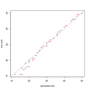
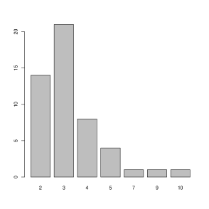
Figure 1: Simulation results from 50 random data sets of dimension n=2000, p=5000 , $d^{*}\stackrel{{\scriptstyle\mathrm{iid}}}{{\sim}}\mbox{Uniform}[10,50]$, $\kappa=2$. Left panel reports the estimates of $\hat{d}^{*}$ vs the true rank $d^{*}$. The right panel reports the selected vaues for $t^{*}$.

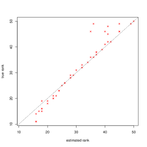
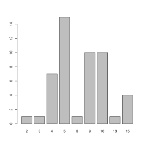
Figure 2: Simulation results from 50 random data sets of dimension n=2000, p=5000 , $d^{*}\stackrel{{\scriptstyle\mathrm{iid}}}{{\sim}}\mbox{Uniform}[10,50]$, $\kappa=1$. Left panel reports the estimates of $\hat{d}^{*}$ vs the true rank $d^{*}$. The right panel reports the selected vaues for $t^{*}$.

3.1.2 Supervised dimension reduction

Classification example.

This section demonstrates the performance of the dimension reduction approaches on the XOR classification example. Our particular simulation setup is a generalization from (Wu et al., 2010), Section 4. The first $d^{*}$ dimensions of the simulated data contain axis-aligned signal which is centered around $(\pm 2,\pm 2)$ and symmetric about 0 with added isotropic Gaussian noise. All remaining dimensions contain only Gaussian noise (see Figure 6 in the Appendix for an example of $d^{*}=4$). In order to study the classification performance of the dimension reduction methods we generate data with $d^{*}=10$ and for $i\in\{1,\ldots,n\}$:

$$X_{ij} = \nu_{i}+\pi\delta_{-2}(X_{ij})+(1-\pi)\delta_{2}(X_{ij}),\ \ \ \mbox{for}\ j\in\{1,\ldots,d^{*}\}$$ (4)

$$X_{ij} = \nu_{i},\ \ \ \mbox{for}\ j>d^{*}$$ (5)

$$\nu_{i} \stackrel{{\scriptstyle\mathrm{iid}}}{{\sim}} N(0,\sigma),$$ (6)

where $\pi=0.5$ and $\sigma$ controls the signal-to-noise relationships. We investigate the classification performance of $k$-nearest neighbor classifier applied to the projected data onto the estimates of the dimension reduction directions based on different reduction methods. To evaluate the classification accuracy we average across values for $k$ ranging from 10% to 30% of the number of samples within each of the 10 distinct clusters (step 2 between consecutive values). In the case of LSIR we set the number of nearest neighbors for the smoothing step to be 20% of the samples within each cluster. The methods we focus on are: SIR and LSIR as implement by the (randomized) Algorithm 1, denoted as sir and lsir, respectively. Whenever randomization is used we refer to the LSIR methods as rand.lsir. The Gaussian Random projections, rand.proj, and oracle (dimension reduction directions known) are included to serve as a reference.

Results.

Figure 3 illustrates the results when $p\ll n$ and $n\ll p$, respectively, focusing on the estimation accuracy for different values of the variance of the Gaussian noise $\sigma^{2}$ (on logarithmic scale). LSIR without randomization performs better than the SIR methods, as expected, which is particularly evident in the data-rich scenario. LSIR with randomization performs better than all other methods in both sample size regimes, with a particularly large improvement in the data-poor scenario. In (Wu et al., 2010), Section 4, LSIR with ridge regularization performed well in a similar setting, however here we observe that rand.lsir performs well even without adding such term.

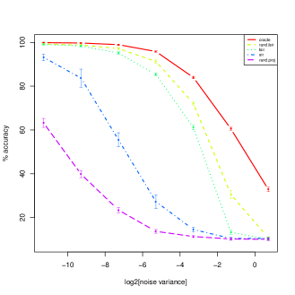
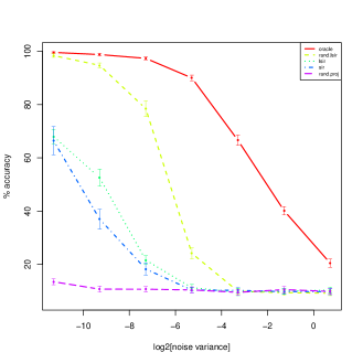
Figure 3: Simulation results from 20 random data sets with signal dimension of XOR $d^{*}=10$. The left panel reports the estimates for ambient dimension is $n=1000,p=200$. The right panel reports the estimates for $n=200,p=1000$. Error bars are based on 2 standard errors of the sample mean.

Latent factor regression model

In this section we explore the accuracy of randomized dimension reduction methods in the setting of factor regression. The modeling assumption is that the response variable $Y$ is strongly correlated with a few directions in covariate space $X$. We compare the proposed estimators with and without randomization. In the latter case we apply full SVD factorization to the input matrices. The methods we focus on are: SIR and LSIR as implement by the (randomized) Algorithm 1, denoted as sir and lsir, respectively. Whenever randomization is used we refer to the methods as rand.sir and rand.lsir. PCA is denoted as pca, and (randomized) PCA as implemented by the Algorithm 2.4 by rand.pca. We will use a latent factor regression model (West, 2003) to simulate the data used to evaluate the performance of the different methods. The rationale behind using a latent factor regression model is that we have explicit control of the direction of variation in covariates space $X$ which is strongly correlated with the response $Y$. The latent factor model corresponds to the following decomposition

$$Y_{i} = \lambda_{i}^{T}\theta+\epsilon_{i},$$

$$X_{i} = BS\lambda_{i}+\nu_{i},$$

where $B\in\mathbb{R}^{p\times d^{*}}$, $B^{T}B=I_{d^{*}}$, and $S=\mbox{diag}(s_{1},\ldots,s_{d^{*}})$ and $d^{*}\ll p$. The random variables $\lambda_{i},\nu_{i},\epsilon_{i}$ are independent and normally distributed

$$\begin{pmatrix}\lambda_{i}\\ \epsilon_{i}\\ \nu_{i}\end{pmatrix}\sim\mbox{N}(0,V),\ \ V=\begin{pmatrix}I_{d^{*}}&0&0\\ 0&\tau^{2}&0\\ 0&0&\psi^{2}I_{p}\end{pmatrix}.$$

Under the above model as the noise in the covariates decreases ($\psi^{2}\rightarrow 0$), we obtain

$$Y_{i}\mid x_{i} \sim \mbox{N}(x_{i}^{T}BS^{-1}\theta,\tau^{2}),$$

which corresponds to the principal components regression model

$$Y_{i}\mid x_{i}\sim\mbox{N}(\tilde{x}_{i}\tilde{\theta},\tau^{2}),\quad\mbox{with }\tilde{x}_{i}=B^{T}x_{i}\mbox{ and }\tilde{\theta}=S^{-1}\theta.$$

The dependence between $X_{i}$ and $Y_{i}$ is induced by marginalizing the latent factors $\lambda_{i}$. The joint distribution for $(Y_{i},X_{i})$ is normal

$$\begin{pmatrix}X_{i}\\ Y_{i}\end{pmatrix}\sim\mbox{N}(0,\Sigma),\ \ \Sigma=\begin{pmatrix}BS^{2}B^{T}+\psi^{2}I&BS\theta\\ \theta^{T}SB^{T}&\tau^{2}+\theta^{T}\theta\end{pmatrix},$$

as is the conditional

$$Y_{i}\mid x_{i},\theta,S,\sim\mbox{N}\left(\theta^{T}SB^{T}Cx_{i},\tau^{2}+\theta^{T}(I-SB^{T}CBS)\theta\right),\quad C=(BS^{2}B^{T}+\psi^{2}I)^{-1}\in\mathbb{R}^{p}.$$

For the above model the parameters $\psi^{2}$ and $\tau^{2}$ control the percentage of variance explained or signal-to-noise

$$\mbox{s}2\mbox{n}_{x}=\frac{\min(s_{i}^{2})}{\psi^{2}+\min(s_{i}^{2})},\quad\mbox{s}2\mbox{n}_{y}=\frac{\theta^{T}\theta}{\tau^{2}+\theta^{T}\theta}=\frac{\mbox{Var}(\lambda^{T}_{i}\theta)}{\mbox{Var}(Y_{i})}.$$

We focus on two signal-to-noise regimes, setting both parameters to vary uniformly at random between (A) 0.6 and 0.9 – strong signal, and (B) 0.3 and 0.6 – weak signal. In both simulation scenarios we set the dominant directions of variation in the covariates to correlate with the regression coefficient. In particular, the parameters $\{\theta_{i}\}$ and $\{s_{i}\}$ are drawn from a t-distribution with 5 degrees of freedom, with the eigenvalue directions assigned such that $|\theta_{1}|>|\theta_{2}|>\ldots>|\theta_{d^{*}}|$ and $|s_{1}|>|s_{2}|>\ldots>|s_{d^{*}}|$. The the number of factors is random, $d^{*}\stackrel{{\scriptstyle\mathrm{iid}}}{{\sim}}\mbox{Uniform}[5,20]$, and the covariance structure is set to be spherical $\psi^{2}I$.

Evaluation criteria.

We used three criteria to evaluate the estimates of the projection direction we obtained from the different methods. The first was the absolute value of the correlation of the dimension reduction space which in our simulations was the vector

$$b=S_{Y|X}=\mbox{span}[{\rm Cov}(X)^{-1}{\rm Cov}(X,Y)]=\mbox{span}[(BS^{2}B^{T}+\psi^{2}I)^{-1}BS\theta].$$

We report the absolute correlation (AEDR) of $b$ with the effective dimension reduction estimate $\hat{b}$, $|\mbox{corr}(b,\hat{b})|$. The second and third metric are based on predictive criteria. In the first case the criterion used is an estimate of the mean square prediction error (MSPE)

$$E\|Y-Z\hat{b}\|^{2}_{2},$$

where $Z$ is the projection of the data $X$ onto the edr subspace and $\hat{b}$ are the regression coefficients estimates. The third metric is the proportion of the variance explained by the linear regression ($R^{2}$), $\mbox{Cor}(Y,\hat{Y})^{2}$, where $\hat{Y}=Z\hat{b}.$ We generated $20$ data sets. The performance on the different evaluation criteria was estimated using test data generated from the same simulation setup as the training data:

$$\lambda^{*}_{i}\stackrel{{\scriptstyle\mathrm{iid}}}{{\sim}}N(0,I_{d^{*}}),\ \epsilon^{*}_{i}\stackrel{{\scriptstyle\mathrm{iid}}}{{\sim}}N(0,\tau^{2}),\ \nu^{*}_{i}\stackrel{{\scriptstyle\mathrm{iid}}}{{\sim}}N(0,\psi^{2}I_{p})$$

$$Y_{test,i}=\lambda_{i}^{*T}\theta+\epsilon^{*}_{i},\ \ \ X_{test,i}=BS\lambda^{*}_{i}+\nu^{*}_{i}.$$

For each of the two parameter settings we examined two data size regimes, $n>p$ and $p>n$. For the LSIR and SIR algorithms the number of slices is set to ten, $H=10$, and for LSIR the nearest neighbor parameter is set to ten, $k=10$. The rank of edr subspace is set for all algorithms to the true value $r=d^{*}=1$. For all randomized methods we use the adaptive strategy described in Section 2.4.1 to estimate the value for $t^{*}$.

Results.

Table 3 and 4 report the results for the various dimension reduction approaches methods in the case of high signal-to-noise ($\mbox{s}2\mbox{n}_{x},\mbox{s}2\mbox{n}_{y}\stackrel{{\scriptstyle\mathrm{iid}}}{{\sim}}\mbox{Uniform}[0.6,0.9]$) and low signal-to-noise ($\mbox{s}2\mbox{n}_{x},\mbox{s}2\mbox{n}_{y}\stackrel{{\scriptstyle\mathrm{iid}}}{{\sim}}\mbox{Uniform}[0.3,0.6]$) for both $n>p$ and $n<p$. In all cases the supervised methods outperform PCA-based methods. Interestingly, randomization tends to be beneficial in the data-poor regime, irrespective of the signal-to-noise ratio. In the setting where the regression signal is low compared to the noise and the sample size is small (Table 4), randomization seems to have the strongest positive effect. It improves both the predictive performance as well as the estimate of the true edr for SIR and LSIR. It is known that LSIR tends to perform much better with added regularization term (Wu et al., 2010). But we observe that factorizing $\hat{\Gamma}$ instead of $\hat{\Sigma}$, which is the typical approach adopted in other LSIR solutions, seems to alleviate this problem. This seems to be the case in the data-rich regime, where lsir performs well without extra regularization.

	Low signal-to-noise			High signal-to-noise
Method	$R^{2}$	MSPE	AEDR	$R^{2}$	MSPE	AEDR
sir	$\bf{0.45\pm 0.02}$	$\bf{1.04\pm 0.01}$	$0.54\pm 0.05$	$\bf{0.75\pm 0.02}$	$\bf{1.16\pm 0.03}$	$\bf{0.56\pm 0.05}$
rand.sir	$0.37\pm 0.02$	$1.20\pm 0.03$	$\bf{0.57\pm 0.04}$	$0.57\pm 0.03$	$2.12\pm 0.16$	$0.53\pm 0.05$
lsir	$0.33\pm 0.02$	$1.27\pm 0.03$	$0.10\pm 0.02$	$0.64\pm 0.03$	$1.67\pm 0.12$	$0.18\pm 0.03$
rand.lsir	$0.22\pm 0.02$	$1.49\pm 0.05$	$0.35\pm 0.04$	$0.40\pm 0.03$	$2.97\pm 0.22$	$0.35\pm 0.04$
pca	$0.19\pm 0.02$	$1.56\pm 0.06$	$0.29\pm 0.04$	$0.32\pm 0.03$	$3.48\pm 0.29$	$0.27\pm 0.03$
rand.pca	$0.19\pm 0.01$	$1.56\pm 0.05$	$0.30\pm 0.04$	$0.28\pm 0.03$	$3.69\pm 0.31$	$0.24\pm 0.03$

Table 3: Estimates of the mean performance and its standard error based on the Latent Factor Regression model. The results are based on 20 replicate data sets of dimension $n=3000$, $p=500$.

	Low signal-to-noise			High signal-to-noise
Method	$R^{2}$	MSPE	AEDR	$R^{2}$	MSPE	AEDR
sir	$0.15\pm 0.05$	$1.58\pm 0.10$	$0.16\pm 0.05$	$0.32\pm 0.08$	$3.23\pm 0.49$	$0.26\pm 0.07$
rand.sir	$\bf{0.34\pm 0.02}$	$\bf{1.22\pm 0.04}$	$\bf{0.56\pm 0.04}$	$\bf{0.58\pm 0.03}$	$\bf{1.84\pm 0.12}$	$\bf{0.57\pm 0.06}$
lsir	$0.09\pm 0.02$	$1.74\pm 0.07$	$0.03\pm 0.01$	$0.16\pm 0.04$	$4.28\pm 0.40$	$0.03\pm 0.01$
rand.lsir	$0.28\pm 0.03$	$1.34\pm 0.06$	$0.46\pm 0.05$	$0.50\pm 0.04$	$2.23\pm 0.18$	$0.48\pm 0.06$
pca	$0.20\pm 0.03$	$1.50\pm 0.06$	$0.31\pm 0.04$	$0.35\pm 0.03$	$3.03\pm 0.26$	$0.31\pm 0.04$
rand.pca	$0.20\pm 0.03$	$1.50\pm 0.06$	$0.32\pm 0.04$	$0.36\pm 0.03$	$3.00\pm 0.26$	$0.31\pm 0.04$

Table 4: Estimates of the mean performance and its standard error based on the Latent Factor Regression model. The results are based on 20 replicate data sets of dimension $n=500$, $p=3000$.

3.2 Real data

In this section we evaluate the predictive performance of kNN classifiers after dimension reduction by the proposed supervised and unsupervised approaches. Our evaluation metric is the % classification accuracy. In all data analyses we set the number of slices for SIR and LSIR to be $H=10$ and assume that the dimension of the reduction subspace equals the rank of $\Gamma$.

3.2.1 Digit Recognition

The first data set we consider contains 60,000 digital images of handwritten grey-scale digits from MNIST. This data set has been extensively studied in the past and has been found to contain non-linear structure. Each image has dimensions $28\times 28$, which we represent in a vectorized form, ignoring the spatial dependencies among neighboring pixels. Hence $p=28\times 28=784$. After removing the pixels that have constant values across all sample images, the dimension becomes $p=717$. For more details regarding the data refer to the Appendix. The dimension reduction methods we compare are pca, sir, lsir, and rand.lsir, and use as a baseline reference Gaussian random projections (rand.proj). The value for $t^{*}$ is estimated from the data, assuming fixed value for the rank of $\Gamma$, $d^{*}$ (see Section 2.4.1). We fix the neighborhood size to be 10 for both the accuracy evaluation and the slice estimation for LSIR. Each training set consists equal number of randomly selected images of each digit and each test set is constructed in identical fashion.

Results.

The performance results for different ranks of $\Gamma$ are summarized in Figure 4. We use n=50 and n=100 training examples for each of the digits between 0 and 9. Note that SIR can estimate up to 9 edrs (# classes - 1), while LSIR-based approches do not have that limitation, so we report results allowing for the number of edrs to vary from 1 to 15 (fixing it at at a maximum of 9 for SIR). Randomized LSIR tends to perform the best for smaller number of edrs, with SIR and pca catching up as the number increases. Also, LSIR seems to be prone to overfitting and its performance improves with increased sample size.

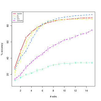
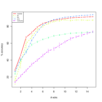
Figure 4: Simulation results from 10 random data sets of size 50 (left panel) and 100 (right panel) randomly selected samples for each digit. Hence the total sample size is $n=500$ and $n=1000$, respectively. Each sample image is of dimension $p=717$. The error bars are based on 2 standard errors of the sample mean.

3.2.2 HapMap gene expression data

In this section we evaluate the classification accuracy of different approaches on a microarray gene expression data set from (Stranger et al., 2012) for the purposes of e-QTL analysis, associating genetic variants to variation in the gene expression. Our focus is only on the gene expression data, using the pre-processed values as features to classify the individual samples to their respective population of origin. The data set consists of gene expression data from lymphoblastoid blood cells assayed in 728 individuals from 8 world populations (HapMap3): western Europe 112, Nigeria 108, China 80, Japan 82, India 81, Mexico 45, Maasai Kenya 137, Lihua Kenya 83. After pre-processing of the data for potential technical artifacts we use as input for the analysis 12,164 gene features. For more details regarding the pre-processing of the data refer to the Appendix HapMap microarray gene expression data. We set the neighborhood size to be 10 for both the accuracy evaluation and the slice estimation for LSIR. The value of $t^{*}$ is estimated from the data (see Section 2.4.1) and the classification accuracy is reported over a range of values for the number edrs.

Results.

Figure 5 contains estimates of the estimation accuracy for different number of dimension reduction directions. The estimates are based on 10 random splits of the data into equally sized train and test set. All approaches show large improvement upon the baseline random projection reference. Clearly, rand.lsir and lsir outperform sir and pca, suggesting that there may be strong non-linear structure in the gene expression data, which is predictive of the population of origin. In additon, similarly to the digits data example from Section 3.2.1, for smaller number of edrs the randomizated version of LSIR seems to produce the best classification performance, which becomes comparable to LSIR as the number of edrs increases. This suggests a potential advantage of randomized methods if a more parsimonious dimension reduction model, with few edrs, is to be estimated.

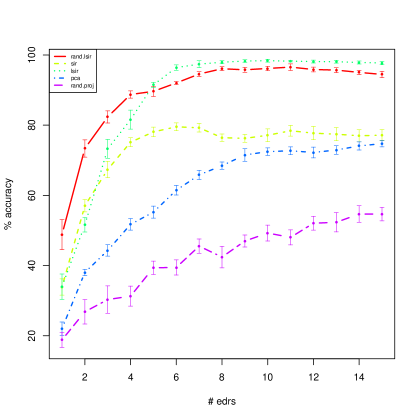
Figure 5: Classifiction accuracy of the k-nearest neighbor classifier applied to microarray gene expression data from 8 HapMap populations stratified by population. $n=728$, $p=12,164$. The results are based on 10 random splits of the data into train and test set of equal sizes. The x-axis contains the number of dimension reduction directions used to project the data.

4 Discussion

Massive high dimensional data sets are ubiquitous in modern applications. In this paper we address the problem of reducing the dimensionality, in order to extract the relevant information, when analyzing such data. The main computational tool we use is based on recent randomized algorithms developed by the numerical analysis community. Taking into account the presence of noise in the data we provide an adaptive method for estimation of both the rank $d^{*}$ and number of Krylov iterations $t^{*}$ for the randomized approximate version of SVD. Using this adaptive estimator of low-rank structure, we implement efficient algorithms for PCA and two popular semi-parametric supervised dimension reduction methods – SIR and LSIR. Perhaps, the most interesting statistical observation is related to the implicit regularization which randomization seems to impose on the resulting estimates. Some important open questions still remain:

1. There is need for a theoretical framework to quantify what generalization guarantees the randomization algorithm can provide on out-of-sample data and the dependence of this bound on the noise and the structure in the data on one hand and on the parameters of the algorithms on the other;

2. A probabilistic interpretation of the algorithm could contribute additional insights into the practical utility of the proposed approach under different assumptions. In particular it would be interesting to relate our work to a Bayesian model with posterior modes that correspond to the subspaces estimated by the randomized approach.

Appendix

Randomized algorithms for dimension reduction

Algorithm 1 : Randomized (L)SIR

input: $X\in\mathbb{R}^{n\times p}$: data matrix
$H$: number of slices
$k$: number of nearest neighbors [LSIR only]
$d_{\max}$: upper bound for the dimension of the projection subspace (can provide a fixed value instead: $\hat{d}^{*}\equiv d^{*}$)
$\Delta$: oversampling parameter for the Adaptive Randomized SVD step   [default: $\Delta=10$]
$t_{\max}$: upper bound for the number of power iterations for the Adaptive Randomized SVD step (can provide a fixed value instead)
output: $\hat{G}_{(L)SIR}\in\mathbb{R}^{p\times\hat{d}^{*}}$: a basis matrix for the effective dimension reduction subspace

Stage 1: Estimate low-rank approximation to $\hat{\Gamma}_{(L)SIR}$

1. Construct   $J_{(L)SIR}$, as described in Section 2.5.3

2. Set   $L=X^{T}J_{(L)SIR}^{T}\ \ (\Rightarrow\hat{\Gamma}_{(L)SIR}=LL^{T})$

3. Factorize & estimate rank   {$[U,S,V]$, $\hat{d}^{*}$} = $\textit{Adaptive Randomized SVD}(L,t_{\max},d_{\max},\Delta)$

Stage 2: Solve the generalized eigendecomposition

1. Construct   $A=SU^{T}X^{T}\in\mathbb{R}^{\hat{d}^{*}\times p}$

2. Factorize   $[\tilde{U},\tilde{S},\tilde{V}]=\text{full SVD(A)}$

3. Back-transform   $\hat{G}_{(L)SIR}=\tilde{U}SU^{T}\in\mathbb{R}^{p\times\hat{d}^{*}}$

XOR model

Figure 6 includes an example of n=100 simulated data points from the XOR example described in Section 3.1.2. The number of signal directions $d^{*}=4$. We show the projected data onto the first two coordinate axes.

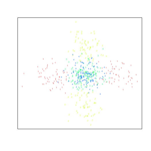
Figure 6: XOR classification example. $n=100,d^{*}=4$. The data is projected onto the first two coordinate directions of $X$.

Digit Recognition

The MNIST data set (Y. LeCun, htpp://yann.lecun.com/exdb/mnist/) (LeCun et al., 1998) contains 60,000 images of handwritten grey-scale digits of dimension $p=28\times 28=784$. It is a subset of a larger set available from NIST. The digits have been size-normalized and centered in a fixed-size image. In our evaluations we use the subset of ’training images’ which is contained in files ’train-images-idx3-ubyte.gz’ ’train-labels-idx1-ubyte.gz’.

HapMap microarray gene expression data

The HapMap microarray gene expression data from from (Stranger et al., 2012) contains 2 replicates per individual, measured using the Illumina’s Sentrix Human-6 Expression BeadChip version 2 whole genome expression array ($\sim$ 48,000 probesets). We use as input to the pre-processing pipeline the background-corrected and summarized (by the Illumina software) probeset intensities, which map to unique genes and is annotated as ’good’ by the thorough re-annotation effort reported in (Barbosa-Morais et al., 2010) (using ENSEMBL gene annotation, release GRCh37/hg19). This corresponds to 12,164 Illumina probeset expression values.

Pre-processing pipeline

This section describes the pre-processing steps for the gene expression data.

1. Impute non-positive probeset entries using the median intensity across all probeset within the same population, independently for the individuals from Rep1 nd Rep2.

2. $log_{2}$-transform all probest measurements.

3. Select probesets marked as ’good’ by the re-annotation of the Illumina microarray data in (Barbosa-Morais et al., 2010).

4. Remove the top variance direction of the difference between technical replicates: Rep1-Rep2 from Rep1 and from Rep2 – results in large improvement in the correlation between Rep1 and Rep2 across all samples

5. Average probeset values between Rep1 and Rep2.

Unsupervised dimension reduction

In this section we outline a potential extension of the ideas for randomized dimension reduction developed in the main text to the unsupervised problem of manifold learning. In particular, we focus on Localized Locality Projections (He and Niyogi, 2003), which is a linear relaxation of the Laplacian Eigenmaps method originally introduced in (Belkin and Niyogi, 2003) and allows for easy out-of sample application of the estimated reductions.

Dimension reduction based on graph embeddings (LPP)

Dimension reduction based on graph embeddings seek to map the original data points to a lower dimensional set of points while preserving neighborhood relationships. The theoretical assumptions underlying these methods are that the data lies on a smooth manifold embedded in the high-dimensional ambient space. This manifold is unknown and needs to be inferred from the data. Given sufficient number of observations the manifold can be reasonably represented as a $G=(E,V)$ (Chung, 1997) where the vertexes $\{v_{1},..,v_{n}\}$ correspond to the $n$ observations $\{x_{1},..,x_{n}\}$ and the edges corresponds to points which are close to each other. For example, this neighborhood relationship can be encoded in a sparse symmetric adjacency matrix $W$. Given $W$, the Laplacian Eigenmaps (LE) algorithm (Belkin and Niyogi, 2003) embeds the data into a low dimensional space preserving local relationships between points. Given the adjacency or association matrix the Graph Laplacian is constructed $L=D-W$, where $D$ is a diagonal matrix with $D_{ii}=\sum_{j}W_{ij}$. A spectral decomposition of $L$

$$Lv_{i}=\lambda_{i}v_{i}$$ (7)

results in eigenvalues $\lambda_{1}=0\leq\lambda_{2}\leq...\leq\lambda_{n}$ with $v_{1}=\mathbf{1}$. Projecting the matrix $L$ onto the $d^{*}$ eigenvectors corresponding to the smallest $d^{*}$ eigenvalues greater than zero embeds the $n$ points into a $d^{*}$ dimensional space. Notice that (7) is a special case of (1), with $\Gamma=L$ and $\Sigma=I$. Under certain conditions (Belkin and Niyogi, 2005), the Graph Laplacian converges to the Laplace-Beltrami operator on the underlying manifold. This provides a theoretical motivation for the embedding. This embedding needs to be recomputed when a new data point is introduced and typically will not be a linear projection of the data. Hence, for computational reasons it would be advantageous to have a linear projection that can be applied to new data points without having to recompute the spectral decomposition of the graph Laplacian. The goal of Locality Preserving Projections (He and Niyogi, 2003) is to provide such a linear approximation to the non-linear embedding of Laplacian Eigenmaps (Belkin and Niyogi, 2003). The dimension reduction procedure starts by specifying the dimension of the transformed space to be $d^{*}<n$. Let the parameter defining the neighborhood size be $k$. Locality Preserving Projections (LPP) (He and Niyogi, 2003) is stated as the following generalized eigendecomposition problem.

$$\begin{split}X^{T}LXe&=\lambda X^{T}DXe,\\ X^{T}(D-W)Xe&=\lambda X^{T}DXe,\\ X^{T}WXe&=(1-\lambda)X^{T}DXe,\\ \tilde{X}^{T}\tilde{W}\tilde{X}e&=\mu\tilde{X}^{T}\tilde{X}e,\end{split}$$ (8)

where, $\tilde{X}=D^{\frac{1}{2}}X$, $\tilde{W}=D^{-\frac{1}{2}}WD^{-\frac{1}{2}}$, $\mu=1-\lambda$ and for a fixed bandwidth parameter $b>0$,

$$W_{ij}=\left\{\begin{array}[]{l l}\text{exp}\left\{-\frac{||X_{i}-X_{j}||}{\text{b}}\right\}&\quad\text{if $X_{i}$ is among the $k$-NN of $X_{j}$ or vice versa}\\ 0&\quad\text{otherwise}.\\ \end{array}\right.$$

The column vectors that are the solutions to equation (8) (excluding the trivial solution $e_{0}$) are the required embedding directions $\{e_{j}\}$, ordered according to their generalized eigenvalues $1=\mu_{0}>\mu_{1}>\ldots>\mu_{d^{*}-1}$. Hence the neighborhood-preserving optimal embedding according to the LPP criterion is:

$$x_{i}\rightarrow A^{T}y_{i},\ \ \ \text{where}\ \ A=(e_{1},\ldots,e_{d^{*}}).$$

The formulation (8) is a special case of (1), with $\Gamma=\tilde{X}^{T}\tilde{W}\tilde{X}$ and $\Sigma=\tilde{X}^{T}\tilde{X}$.

LPP Estimation.

The approximation algorithm to solve LPP requires solving the generalized eigendecomposition stated by the last equation in derivation (8). There will be on the order of $kn$ non-zero entries. Hence, the matrix $\tilde{W}$ will be sparse, assuming the size of the local neighborhoods $k\ll n$. This implies that the matrix product $X^{T}WX\Omega$, where $\Omega\in\mathbb{R}^{p\times l}$ can be efficiently computed in $O((k+l)np)$ time, without explicitly constructing $W$ by using the $k$-nearest neighbor matrix. Hence $\tilde{\Gamma}:=\tilde{X}^{T}\tilde{W}\tilde{X}$ can be efficiently approximated using Adaptive Randomized SVD algorithm from Section 2.4 which would provide and estimate for $SU^{T}$. Then, setting $\tilde{\Sigma}:=\tilde{X}^{T}\tilde{X}$, we reduce the problem to (3). Next we describe the randomized LPP algorithm in more detail:

Algorithm 2 : Randomized LPP

input: $X\in\mathbb{R}^{n\times p}$: data matrix
$k$: number of nearest neighbors capturing local manifold structure
$d_{\max}$: upper bound for the dimension of the projection subspace (can provide a fixed value instead)
$\Delta$: oversampling parameter for the Adaptive Randomized SVD step   [default: $\Delta=10$]
$t_{\max}$: upper bound for the number of power iterations for the Adaptive Randomized SVD step (can provide a fixed value instead)
output: $\hat{G}_{LPP}\in\mathbb{R}^{p\times d^{*}}$: a basis matrix for the embedding subspace

Stage 1: Estimate low-rank approximation to $\tilde{X}^{T}\tilde{W}\tilde{X}$

1. Construct $\tilde{X}$ and $\tilde{W}$,

2. Factorize {$[U,S,U]$, $\hat{d}^{*}$} = $\textit{Adaptive Randomized SVD}(\tilde{X}^{T}\tilde{W}\tilde{X},t_{\max},d_{\max},\Delta)$

Stage 2: Solve the generalized eigendecomposition

1. Construct $A=SU^{T}\tilde{X}^{T}\in\mathbb{R}^{\hat{d}^{*}\times p}$

2. Factorize $[\tilde{U},\tilde{S},\tilde{V}]=\text{full SVD(A)}$

3. Back-transform   $\hat{G}_{LPP}=\tilde{U}SU^{T}\in\mathbb{R}^{p\times\hat{d}^{*}}$

References

- Achlioptas (2001) Achlioptas, D. (2001). Database-friendly random projections. In Proceedings of the twentieth ACM SIGMOD-SIGACT-SIGART symposium on Principles of database systems, PODS ’01, New York, NY, USA, pp. 274–281. ACM.
- Adcock (1878) Adcock, R. (1878). A problem in least squares. The Analyst 5, 53–54.
- Anderson et al. (1990) Anderson, E., Z. Bai, J. Dongarra, A. Greenbaum, A. McKenney, J. Du Croz, S. Hammerling, J. Demmel, C. Bischof, and D. Sorensen (1990). Lapack: a portable linear algebra library for high-performance computers. In Proceedings of the 1990 ACM/IEEE conference on Supercomputing, Supercomputing ’90, Los Alamitos, CA, USA, pp. 2–11. IEEE Computer Society Press.
- Baglama and Reichel (2006) Baglama, J. and L. Reichel (2006). Restarted block lanczos bidiagonalization methods. Numerical Algorithms 43(3), 251–272.
- Barbosa-Morais et al. (2010) Barbosa-Morais, N., M. Dunning, S. Samarajiwa, J. Darot, M. Ritchie, A. Lynch, and S. Tavare (2010). A re-annotation pipeline for Illumina BeadArrays: improving the interpretation of gene expression data. Nucleic Acids Research 38.
- Belkin and Niyogi (2003) Belkin, M. and P. Niyogi (2003). Laplacian eigenmaps for dimensionality reduction and data representation. Neural Computation 15(6), 1373–1396.
- Belkin and Niyogi (2005) Belkin, M. and P. Niyogi (2005). Towards a theoretical foundation for laplacian-based manifold methods.
- Boutsidis et al. (2009) Boutsidis, C., M. W. Mahoney, and P. Drineas (2009). An improved approximation algorithm for the column subset selection problem. In Proceedings of the twentieth Annual ACM-SIAM Symposium on Discrete Algorithms, SODA ’09, pp. 968–977. Society for Industrial and Applied Mathematics.
- Chung (1997) Chung, F. R. K. (1997). Spectral Graph Theory, Volume 92. American Mathematical Society.
- Cook (2007) Cook, R. (2007). Fisher lecture: Dimension reduction in regression. Statistical Science 22(1), 1–26.
- Cook and Weisberg (1991) Cook, R. and S. Weisberg (1991). Disussion of li (1991). J. Amer. Statist. Assoc. 86, 328–332.
- Dasgupta and Gupta (2003) Dasgupta, S. and A. Gupta (2003). An elementary proof of a theorem of johnson and lindenstrauss. Random Structures & Algorithms 22(1), 60–65.
- Donoho and Grimes (2003) Donoho, D. and C. Grimes (2003). Hessian eigenmaps: new locally linear embedding techniques for highdimensional data. PNAS 100, 5591–5596.
- Drineas et al. (2006) Drineas, P., R. Kannan, and M. W. Mahoney (2006, July). Fast monte carlo algorithms for matrices ii: Computing a low-rank approximation to a matrix. SIAM J. Comput. 36, 158–183.
- Edegworth (1884) Edegworth, F. (1884). On the reduction of observations. Philosophical Magazine, 135–141.
- Fisher (1922) Fisher, R. (1922). On the mathematical foundations of theoretical statistics. Philosophical Transactions of the Royal Statistical Society A 222, 309–368.
- Fisher (1936) Fisher, R. (1936). The Use of Multiple Measurements in Taxonomic Problems. Annals of Eugenics 7(2), 179–188.
- Frankl and Maehara (1987) Frankl, P. and H. Maehara (1987, June). The johnson-lindenstrauss lemma and the sphericity of some graphs. J. Comb. Theory Ser. A 44, 355–362.
- Gabriel (2002) Gabriel, K. R. (2002). Le biplot - outil d’exploration de donn es multidimensionnelles. Journal de la soci t fran aise de statistique 143(3-4), 5–55.
- Golub et al. (2000) Golub, G., K. S lna, and P. V. Dooren (2000). Computing the svd of a general matrix product/quotient. SIAM J. Matrix Anal. Appl 22, 1–19.
- Golub (1969) Golub, G. H. (1969). Matrix decompositions and statistical calculations. Technical report, Stanford, CA, USA.
- Golub and Van Loan (1996) Golub, G. H. and C. F. Van Loan (1996). Matrix computations (3rd ed.). Baltimore, MD: John Hopkins University Press.
- Gu and Eisenstat (1996) Gu, M. and S. C. Eisenstat (1996, July). Efficient algorithms for computing a strong rank-revealing qr factorization. SIAM J. Sci. Comput. 17(4), 848–869.
- Halko et al. (2009) Halko, N., P. Martinsson, and J. A. Tropp (2009, September). Finding structure with randomness: Probabilistic algorithms for constructing approximate matrix decompositions. ArXiv e-prints.
- He and Niyogi (2003) He, X. and P. Niyogi (2003). Locality preserving projections. In NIPS.
- Hotelling (1933) Hotelling, H. (1933). Analysis of a complex of statistical variables in principal components. Journal of Educational Psychology 24, 417–441.
- Indyk and Motwani (1998) Indyk, P. and R. Motwani (1998). Approximate nearest neighbors: towards removing the curse of dimensionality. In Proceedings of the thirtieth annual ACM symposium on Theory of computing, STOC ’98, New York, NY, USA, pp. 604–613. ACM.
- Johnson and Lindenstrauss (1984) Johnson, W. and J. Lindenstrauss (1984). Extensions of Lipschitz mappings into a Hilbert space. In Conference in modern analysis and probability (New Haven, Conn., 1982), Volume 26 of Contemporary Mathematics, pp. 189–206. American Mathematical Society.
- LeCun et al. (1998) LeCun, Y., L. Bottou, Y. Bengio, and P. Haffner (1998, November). Gradient-based learning applied to document recognition. Proceedings of the IEEE 86(11), 2278–2324.
- Lehoucq et al. (1998) Lehoucq, R. R. B., D. D. C. Sorensen, and C.-C. Yang (1998). Arpack User’s Guide: Solution of Large-Scale Eigenvalue Problems With Implicityly Restorted Arnoldi Methods, Volume 6. Siam.
- Li et al. (2005) Li, B., H. Zha, and F. Chiaromonte (2005). Contour regression: A general approach to dimension reduction. The Annals of Statistics 33(4), 1580–1616.
- Li (1991) Li, K. (1991). Sliced inverse regression for dimension reduction (with discussion). J. Amer. Statist. Assoc. 86, 316–342.
- Li (1992) Li, K. C. (1992). On principal hessian directions for data visulization and dimension reduction: another application of stein’s lemma. J. Amer. Statist. Assoc. 87, 1025–1039.
- Liberty et al. (2007) Liberty, E., F. Woolfe, P.-G. Martinsson, V. Rokhlin, and M. Tygert (2007). Randomized algorithms for the low-rank approximation of matrices. Proceedings of the National Academy of Sciences 104(51), 20167–20172.
- Mahoney (2011) Mahoney, M. W. (2011). Randomized algorithms for matrices and data. CoRR abs/1104.5557.
- Martinsson et al. (2010) Martinsson, P., A. Szlam, and M. Tygert (Vancouver, Canada, 2010). Normalized power iterations for the computation of SVD. NIPS workshop on low-rank methods for large-scale machine learning.
- Nilsson et al. (2007) Nilsson, J., F. Sha, and M. Jordan (2007). Regression on manifolds using kernel dimension reduction. In Proceedings of the 24th International Conference on Machine Learning.
- Owen and Perry (2009) Owen, A. B. and P. O. Perry (2009). Bi-cross-validation of the SVD and the nonnegative matrix factorization. The Annals of Applied Statistics 3, 564–594.
- Polson and Scott (2010) Polson, N. G. and J. G. Scott (2010). Shrink globally, act locally: Sparse bayesian regularization and prediction. In Bayesian Statistics 9. Oxford University Press.
- Rokhlin et al. (2009) Rokhlin, V., A. Szlam, and M. Tygert (2009, August). A randomized algorithm for principal component analysis. SIAM J. Matrix Anal. Appl. 31(3), 1100–1124.
- Roweis and Saul (2000) Roweis, S. and L. Saul (2000). Nonlinear dimensionality reduction by locally linear embedding. Science 290, 2323–2326.
- Saad (1992) Saad, Y. (1992). Numerical methods for large eigenvalue problems, Volume 158. SIAM.
- Sarlos (2006) Sarlos, T. (2006, oct.). Improved approximation algorithms for large matrices via random projections. In Foundations of Computer Science, 2006. FOCS ’06. 47th Annual IEEE Symposium on, pp. 143 –152.
- Stewart (2001) Stewart, G. W. (2001). Matrix Algorithms: Volume 2, Eigensystems, Volume 2. Siam.
- Stranger et al. (2012) Stranger, B., S. Montgomery, A. Dimas, L. Parts, O. Stegle, C. E. Ingle, M. Sekowska, G. D. Smith, D. Evans, M. Gutierrez-Arcelus, A. Price, T. Raj, J. Nisbett, A. Nica, C. Beazley, R. Durbin, P. Deloukas, and E. Dermitzakis (2012). Patterns of cis regulatory variation in diverse human populations. PLoS Genetics 8(4), e1002639.
- Sugiyama (2007) Sugiyama, M. (2007). Dimension reduction of multimodal labeled data by local fisher discriminatn analysis. Journal of Machine Learning Research 8, 1027–1061.
- Tenenbaum et al. (2000) Tenenbaum, J., V. de Silva, and J. Langford (2000). A global geometric framework for nonlinear dimensionality reduction. Science 290, 2319–2323.
- West (2003) West, M. (2003). Bayesian Factor Regression Models in the ”Large p, Small n” Paradigm. Bayesian Statistics 7, 723–732.
- Wu et al. (2010) Wu, Q., F. Liang, and S. Mukherjee (2010). Localized sliced inverse regression. Journal of Computational and Graphical Statistics 19(4), 843–860.
- Young (1941) Young, G. (1941). Maximum likelihood estimation and factor analysis. Psychometrika 6, 49–53.