Extracting interstellar diffuse absorption bands from cool star spectra

Abstract

Aims. Interstellar (IS) absorption lines or diffuse bands are usually extracted from early-type star spectra because they are characterized by smooth continua. However this introduces a strong limitation on the number of available targets, and reduces potential studies of the IS matter and the use of absorptions for cloud mapping.

Methods. We have developed a new and automated fitting method appropriate to interstellar absorptions in spectra of cool stars that possess stellar atmospheric parameters. We applied this method to the extraction of three diffuse interstellar bands (DIBs) in high resolution VLT FLAMES/GIRAFFE spectra of red-clump stars from the bulge. By combining all stellar synthetic spectra, HITRAN-LBLRTM atmospheric transmission spectra and diffuse band empirical absorption profiles, we determine the 6196.0, 6204.5, and 6283.8 Å  DIB strength toward the 219 target stars and discuss the sources of uncertainties. In order to test the sensitivity of the DIB extraction, we inter-compare the three results and compare the DIB equivalent widths with the reddening derived from an independent extinction map based on OGLE photometric data. We also derive the three independent color excess E(B-V) estimates based on the DIB strengths and average linear correlation coefficients previously established in the solar neighborhood and compare with the OGLE photometric results.

Results. Most stellar spectra could be well reproduced by the composite stellar, atmospheric and interstellar models. Measurement uncertainties on the EWs are smaller for the broad and strong 6283.8 Å DIB, and are of the order of 10-15 %. Uncertainties on the two narrow and weaker DIBs are larger, as expected, and found to be highly variable from one target to the other. They strongly depend on the star’s radial velocity. DIB-DIB correlations among the three bands demonstrate that a meaningful signal is extracted. For the 6284 and 6204 Å DIBs, the star-to-star variability of the equivalent width (EW) also reflects features of the OGLE extinction map. The three independent extinction estimates deduced from the EWs and solar neighborhood correlation coefficients agree with each other within 20 % only, which probably reflects the fact that they belong to different families. The estimated average color excess is also compatible with the photometric determination.

Conclusions. This work demonstrates the feasibility of the method of ISM DIB extraction in cool star spectra, based on synthetic spectra. It confirms that DIB measurements and local DIB-extinction calibrations can provide rough, first order estimates of the towards distant targets.

1 Introduction

DIBs and interstellar absorption lines have been almost exclusively extracted from early-type star spectra, using the fact that stellar lines are broad, shallow and in limited number, and do not contaminate the IS lines. Their continua can be easily fitted without any need for stellar models. However, this is a strong limiting factor since it reduces considerably the number of potential targets and the information that can be obtained on the source regions of the absorptions and especially the spatial resolution that can be achieved. In the case of the DIBs, it is limiting studies of the DIB response to the radiation field and to the local physical properties within the IS clouds, while such studies are promising tools in the search for the DIB carriers (e.g. Vos et al. , 2011). Moreover, with the advent of stellar spectroscopic surveys at increasing resolution, the use of multi-object spectrographs and the perspective of forthcoming Gaia parallaxes, a large amount of line-of-sight integrated absorption data will become available. Extracting absorption characteristics towards all targets, including cool stars, would allow a better mapping of the galactic ISM, because it would considerably increase the achievable spatial resolution. For such mapping, interstellar lines of atoms, simple molecules, and DIBs are available, since both contain information on the amount of IS matter. While the former are well identified, carriers of the latter remain unknown, despite their early discovery (Herbig, 1995; Jenniskens and Desert, 1994; Salama et al., 1996; Fulara and Krelowski, 2000; Snow and Destree, 2011; Friedman et al., 2011; Hobbs et al., 2008, 2009, e.g.). Still, this lack of carrier identification and the fact that most of them are only weakly correlated with extinction or gas column are not incompatible with their use as tracers of IS clouds in the same way IS lines are used, i.e. the radial gradients of their strengths allow to locate IS clouds in distance and build 3D maps. In some respects, DIBs may be advantageous ISM tracers: they are numerous, thus observable at various instrumental settings, they are often broad, and in general they are unsaturated. Recent data analyses suggest that the average ratios between the DIBS and the extinction do not seem to vary significantly within the first kiloparsec (Friedman et al., 2011; Vos et al., 2011). Finally, making use of cooler stars to extract their strengths reduces the dispersion around the average relationship, because extreme ionizing field effects linked to bright and hot targets are avoided (Raimond et al., 2012). For this reason, extracting DIB information from cool stars would be another improvement as far as mapping is concerned.

Here we present a new method of DIB measurement based on cool star synthetic spectra, and as a test case we apply this technique to three different diffuse bands and 220 targets located in the galactic bulge that have the advantage of possessing a precise determinations of their atmospheric parameters. We selected the 6196.0, 6204.5, and 6283.8 ${\AA}$ DIBs that are the three strongest absorptions contained in the observed spectral interval. Those DIBs have been already widely studied (see e.g. the works of Galazutdinov et al 2002, Cami et al, 1997, Friedman et al, 2011, Vos et al, 2011). We estimate the statistical and systematic uncertainties on the DIB equivalent widths (EWs) and discuss potential improvements. We compare the measured EW angular pattern over the field with an independent mapping of the reddening based on photometric data of stars close to the galactic center (GC). We finally use average DIB-reddening empirical relationships previously established in the Sun vicinity to derive three independent estimates of the reddening towards all targets, inter-compare the three estimates and finally compare with the photometric determination.

This article is organized as follows. Data are presented in section 2. In section 3 we describe the new method of interstellar absorption band extraction and its ingredients. In Section 4, we show the model adjustments for selected target stars and discuss the results. In Section 5, we discuss the relations between the DIBs and between the DIBs and the extinction obtained by photometry. Section 6 presents color excess estimates based on the DIBs and nearby star studies. Finally, we summarize the results and discuss the perspectives in the last section.

2 Data

We used the sample of 219 bulge red clump giants of Hill et al. (2011). Those stars have been observed with FLAMES/GIRAFFE at the VLT and are located within a 12 arcmin radius field in Baade’s Window (l=0.8, b=-4). We used here the spectra obtained with the GIRAFFE HR13 setup, leading to a resolution of R=22500 and a spectral coverage spanning from 6120 to 6405 $\AA$, that contains three well known diffuse bands of this study. The target selection, observations, data reduction and stellar parameters determination are described by Hill et al. (2011). Those stellar parameters were determined by these authors from photometric and spectroscopic data. Here we use the effective temperature, gravity, micro-turbulence and metallicity resulting from their analysis, whose full ranges for the present sample are listed in Table 1. The different exposures were observed within a week interval so that we can neglect at this resolution variations of the radial velocity difference between the telluric and stellar lines and work with the final co-added spectra. Signal-to-noise ratios vary between $\simeq$ 30 and 77 per pixel (the Giraffe pixel-size is 0.07 Å ).

This region benefits from a high resolution differential extinction map that has been derived from the OGLE-II red clump giants photometry by Sumi (2004). Assuming a mean reddening corrected colour for the red clump, Sumi (2004) divided each field in small sub fields, computed the mean observed colour of the red clump in each sub field and derived the reddening E(V-I). The resulting extinction map has a spatial resolution of 33 arcsec in our field. For comparison purposes we have interpolated within the Sumi (2004) reddening grid to infer its value at each target location. Note that Sumi (2004) indicates a potential zero-point offset for Av that may amount to 0.05. The distribution of the target stars is shown superimposed on the Sumi (2004) extinction map in Fig. 1.

Table 1: Stellar parameters. T_eff is the effective temperature. log $g$ is the gravity. $v_{t}$ is the micro-turbulent velocity. $[Fe/H]$ is the metallicity.

parameters	min	max	unit
Teff	4270	5448	K
log $g$	1.97	2.46
vt	0.8	1.8	km/s
$[Fe/H]$	-1.13	0.71

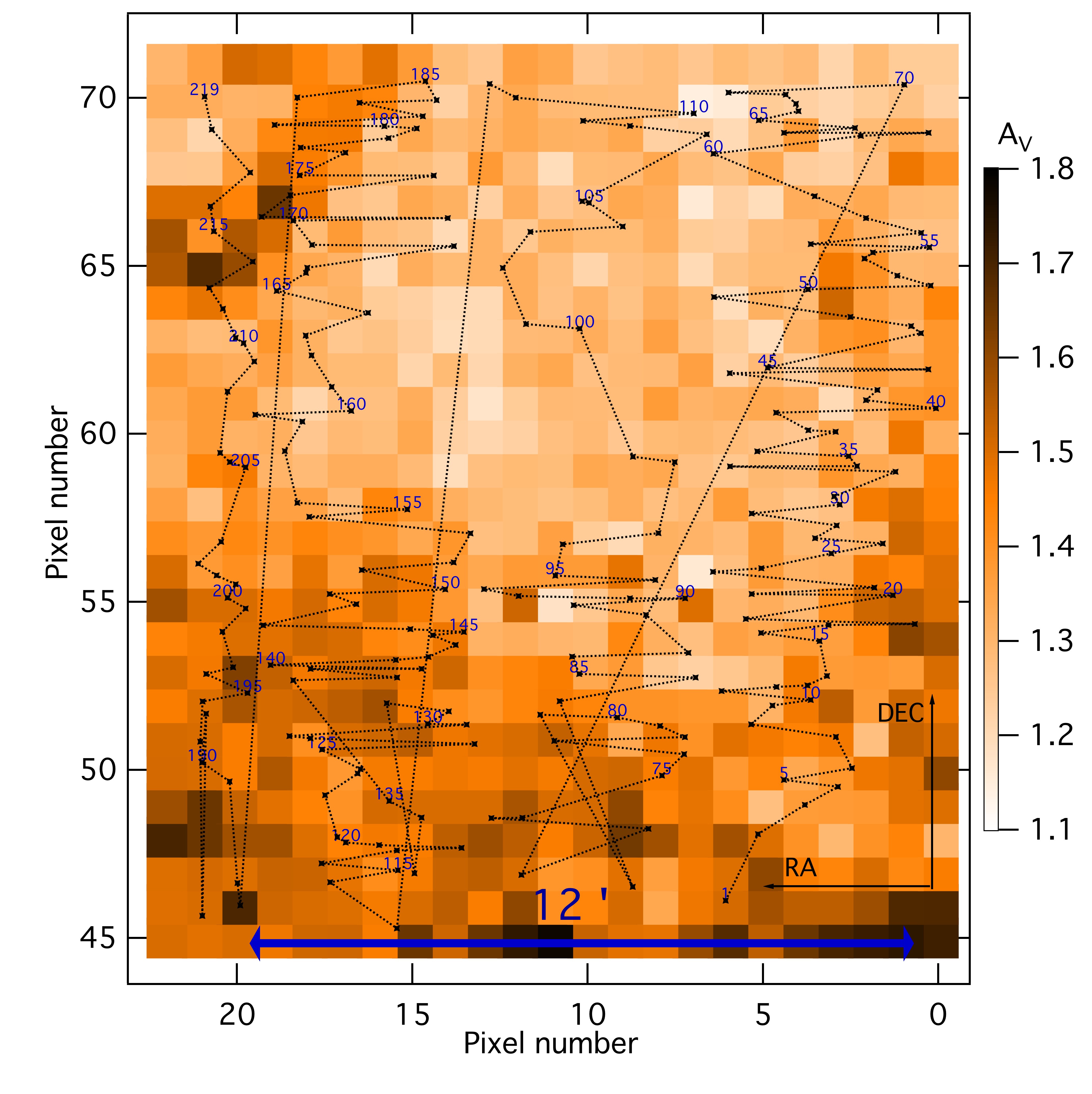
Figure 1: Target stars used in this study (black crosses) superimposed on the extinction map from Sumi (2004). The map is centered on (l,b)=(0.8,-4). Each pixel is 0.6’x0.6’. The extinction scale is displayed in fig 14. Stars are numbered according to Table LABEL:DIB_index. Dotted lines link stars in increasing order of their ID number. Only one out of five numbers is indicated for clarity.

3 Fitting procedure

Our approach is to model and adjust simultaneously the spectrum of the background star, the DIB and the atmospheric transmission in one unique step. In the opposite case of hot stars, extracting the IS absorption was done in two or three steps. The correction for the telluric absorption, if necessary, was done first and independently of the IS absorption fitting. Synthetic transmission spectra were adjusted through computation of the mean ratio between observed and modeled equivalent widths of specific lines (Lallement et al. 1993), or by minimizing the length (defined as the sum of flux differences between consecutive points) of the residual spectrum obtained after dividing by the model atmospheric transmission (Raimond et al. 2012). None of those methods is necessary here, since the atmospheric transmission model is adjusted in velocity and airmass during the global adjustment. In a second step the smooth continuum of the hot star was fitted to a function, and in a last step the DIB strength was measured using the normalized spectrum. Characterizing the DIB strength has been done in several ways, the two main ones being measures of the central depth and of the equivalent width. We refer to the detailed discussion of this point by Friedman et al (2011). We have chosen here the equivalent width, and, as we will see, this is the quantity that directly comes out from our cool star analysis.

In the case of cool stars, the presence of numerous, deep and narrow stellar lines precludes the application of the simple continuum fitting procedure that is used for stars of earlier spectral types. Identifying and correcting the stellar lines one by one in the IS absorption region is not practical. Furthermore, if the stellar lines and the IS absorption do overlap, it is very difficult or even impossible to separate them, hence our approach using a global adjustment. Our composite model here is the product of a synthetic stellar spectrum, a synthetic telluric transmission, and an empirical model for the DIB absorption. The model allows for wavelength shifts between those three spectra to take into account the stellar radial velocity, the Earth motion, and the IS radial velocity. The giant stars used as background sources in the present investigation do not have measurable projected rotational velocities at this resolution. Sizeable projected rotational velocity in the background star could be modelled as well, if necessary. The combination of the three models is convolved by a Gaussian profile to take into account the instrumental spectral resolution and is adjusted to the data in the DIB region, with the DIB strength, the DIB center location, and an atmospheric transmission scaling (see below) being the free parameters.

The synthetic stellar spectra, S($\lambda$), were computed from an ATLAS 9 model atmosphere using the SYNTHE suite (Kurucz 2005). We used the Linux port of all the codes (Sbordone et al. 2004; Sbordone 2005). Atomic and molecular data have been taken from the data base on Kurucz’s website. For each star we computed a synthetic spectrum with the stellar parameters obtained by Hill et al. (2011), i.e. the effective temperatures, gravity, metallicity, and microturbulence, summarized in Table 1. The stellar radial velocity is taken into account by doppler shifting the computed spectrum to the appropriate radial velocity.

The synthetic telluric transmissions are computed by means of the LBLRTM code (Line-By-Line Radiative Transfer Model, Clough et al 2005), using the molecular database HITRAN (HIgh-Resolution TRANsmission molecular absorption, Rothman et al. 2009). Here we have used the transmission T₀($\lambda$) computed for a standard atmosphere and for the altitude of the observatory, and we have assumed that airmass variations from star to star simply result in a variable coefficient $\alpha$ for the transmission, with T($\lambda$) = T₀($\lambda$)^α. The projected Earth motion is taken into account by doppler shifting the transmission.

Finally, the profiles of the 6196.0, 6204.5, and 6283.8 ${\AA}$ DIBs are derived from a high resolution (R=48,000), high signal to noise survey of early-type stars recorded with the FEROS spectrograph at the 2.2m ESO/Max Planck Institute Telescope in La Silla. Those profiles do not reveal the fine structure that is known to be present Galazutdinov et al. (2008) but this is not necessary here since we deal with spectra at a resolution that is lower than the one of FEROS. The shape of the 6283.8 ${\AA}$ DIB, which is contaminated by strong telluric molecular oxygen lines, has been derived by Raimond et al. (2102) by averaging a large number of individual shapes obtained after division by an adjusted telluric template. Such a use of a synthetic atmospheric model is allowed by the fact that this DIB is relatively strong and much broader than the telluric lines. In the same way, this DIB is here broader than the stellar lines and thus relatively easy to detect and measure (see figures 3, 4,5). The two, much weaker DIBs 6196.0 and 6204.5 ${\AA}$ are in regions that are free of contaminating telluric lines. Their shapes have been derived by means of an automated fitting method appropriate for early-type stars (Puspitarini and Lallement, 2012). About ten individual profiles extracted from the best FEROS spectra have been averaged to produce those templates. Since those two DIBs are narrower than the 6283.8 ${\AA}$ DIB, here in the case of cool stars they are much more difficult to measure due to the overlap with the similarly narrow stellar lines.

Neglecting emissions from the cloud in comparison with the stellar flux, DIB transmission profiles D($\lambda$) can be expressed as exp(-$\tau(\lambda))$, where $\tau(\lambda)$ is the optical thickness as a function of wavelength. $\tau(\lambda)$ is proportional to the column N of absorbers and can be expressed as $\tau(\lambda)=N/N_{0}\tau_{0}(\lambda)$, $\tau_{0}(\lambda)$ and $N_{0}$ being some related optical thickness and column of reference. Calling $\beta$ the $N/N_{0}$ ratio, a quantity proportional to the column density of the DIB carrier, one has:

D($\lambda$)=D${}_{0}(\lambda_{D})^{\beta}$, where D₀($\lambda$) = exp(-$\tau_{0}(\lambda))$ is the reference profile derived from the FEROS analyses, and $\lambda_{D}$ is the wavelength shifted by the radial velocity of the main absorbing medium. The DIB equivalent width is by definition:

$$W=\int\frac{I_{0}(\lambda)-I(\lambda)}{I_{0}(\lambda)}d\lambda=\int(1-exp(-\tau(\lambda)))d\lambda$$ (1)

where $I_{0}(\lambda)$ and $I(\lambda)$ are the unabsorbed and absorbed intensities. Within the weak absorption regime appropriate here, $\tau$ is small, $exp(-\tau)\simeq 1-\tau$ and the equivalent width W is approximated by

$$W=\int\tau(\lambda)d\lambda=\int\beta\tau_{0}(\lambda)d\lambda=\beta W_{0}$$ (2)

where $W_{0}$ is the equivalent width of the line of reference.

We have chosen to list the results under the form of the product $\beta W_{0}$, which has the advantage of being both truly proportional to the absorbing column and to be an equivalent width, i.e. widely used, meaningful quantity. For the broader DIB, 6284 Å  the relative difference between $\beta W_{0}$ and the actual EW is here smaller than 4.5 % , a value reached for equivalent widths of the order of 1.2 Å . For the narrower DIB, 6196 Å  the departure from the linear regime for the EW occurs at a smaller optical thickness, however the DIB is weak, and finally the relative difference between $\beta W_{0}$ and the actual EW is smaller than 4. % , a value reached for equivalent widths of the order of 70 mÅ .

After adjustment of the coefficient $\beta$ through spectral fitting, the DIB equivalent width is thus simply computed as the product of the equivalent width of the reference profile $W_{0}$ by the coefficient $\beta$. We also assume here that most of the absorbing medium originates from clouds with a similar radial motion, or equivalently that the DIB is negligibly broadened by the line-of-sight velocity structure. This assumption is legitimated here by the fact that most of the absorption arises within 1,500 pc from the Sun, as derived from the extinction model of Marshall et al. (2006) and that for those low l,b coordinates the projection of the gas motions onto the line-of-sight remains small with respect to the DIB spectral width.

Figure 2 illustrates the procedure for this study. The stellar parameters are used as input for the stellar synthetic models and the stellar radial velocity is taken into account by an appropriate shift. The atmospheric synthetic model of reference is calculated based on the position and altitude of the observatory. While doing the fitting, the program computes the product $\kappa$ S($\lambda_{S}$) T${}_{0}(\lambda_{E})^{\alpha}$ D${}_{0}(\lambda_{D})^{\beta}$, with $\kappa$ being a scaling factor, $\lambda_{S}$ is the wavelength shifted by the stellar radial velocity, $\lambda_{E}$ by the Earth’s radial velocity and $\lambda_{D}$ by the radial velocity of the DIB absorbing medium, and convolves the product of the three models by a Gaussian instrumental function appropriate for the resolution of GIRAFFE .

Telluric absorptions should be identical for all fibers for the same exposure, and we also expect the DIB radial velocity to vary very little over the narrow field. Still, in order to test the adjustment and allow for small uncertainties in the three wavelength shifts, we started by allowing all parameters $\kappa$, $\alpha$, $\beta$, $\lambda_{S}$, $\lambda_{E}$ and $\lambda_{D}$ to freely vary, and performed a least mean squares adjustment to the data for each star. All the fittings were done in an automated way. The results revealed a large majority of identical or very close values for the $\lambda_{E}$ shift (actually a null value for a fit in the earth frame) and for $\alpha$. As mentioned previously this was expected for both $\alpha$, that responds to the airmass, and $\lambda_{E}$ that is a function of the date. We extracted those two parameters and kept them fixed for the second adjustment phase. We could also check from this first attempt that the values found by fitting for $\lambda_{S}$ differ from the radial velocities from Hill et al. (2011) by very small velocity intervals (of the order of 1 km s^-1). We kept those very small differences from values in Table LABEL:DIB_index and fixed $\lambda_{S}$ for the next step. Finally, the coefficient $\lambda_{D}$ that represents the DIB shift was also found to be the same or nearly the same for a large majority of the stars. This confirms that over such a small field of view the DIB radial velocity variation is very small, both because most of the absorption originates from the first two kpc, and also because the radial motion of the absorbing gas in this direction is small. We then fixed this shift $\lambda_{D}$ at the most frequently found value. For all those four parameters we checked that the outliers were corresponding to low signal-to-noise spectra or to the presence of a spurious feature. We then proceeded to a second fit of all spectra, this time for free $\kappa$ and $\beta$ coefficients only.

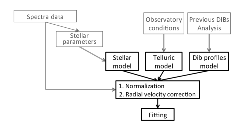
Figure 2: The procedure flowchart of the fitting.

4 Model adjustments

Figures 3, 4 and 5 illustrate exemplary cases of model adjustments for the three 6196.0, 6204.5, and 6283.8 $\AA$ DIBs chosen for this study. In each figure the lower panel shows the model components after optimization of the parameters, i.e. the synthetic stellar model (yellow line), the synthetic atmospheric model (blue line), and the adjusted DIB profile (green line). The upper panel shows the spectra (red line) and the fitting result (purple line). What we aim at showing in those figures are the strong differences linked to the target star individual radial velocities, that vary over a very large velocity interval, from -230 to +250 km.s^-1. This results in very different locations of the DIBs with respect to the main stellar lines. There are also very large differences between the 6283.8 $\AA$ DIB and the two narrow ones, with a much stronger impact of the star radial velocity and of the signal to noise on the DIB detection for the latter two DIBs. Finally, the larger the metallicity, the stronger the stellar lines and their impact on the DIB measurement, especially again in the case of the two narrow and weak DIBs.

Figures 3 to 5 show three examples of adjustments for the strongest and broadest DIB at 6283.8 $\AA$, The first star (Fig. 3) corresponds to an optimal case: given the star radial velocity, only weak stellar lines are located in the DIB region, and the fitting program could easily adjust the DIB strength. Moreover, the star is metal-poor (Fe/H = -0.68), which further helps the fitting procedure. Figures 4 and 5 correspond to more difficult cases, with one or more strong stellar lines in the DIB region. In those cases, provided the stellar models adequately predict the stellar line depths, there should not be difficulties in measuring the DIB strengths with accuracy. However, it can be seen that there are for some spectral regions significant and often systematic differences between the observed and modeled lines. Such departures may have several origins: the oscillator strengths and other atomic data (wavelengths, damping constants) that we use have an error attached to them, some of the lines are simply not identified and absent from our line list, our spectra are computed assuming Local Thermodynamic equilibrium (LTE), departures from LTE in the stellar atmosphere may change the line strength, for a given abundance, the model atmospheres we used are one dimensional static and plane parallel, hydrodynamic effects (granulation) may also have effects both on the line strengths and shapes. In practice our computed stellar spectrum differs from the observed spectrum due to a number of shortcomings in our modelling. For example, significant residuals are found at the locations of unidentified lines of the solar spectrum, like the 6273.949, 6282.816, 6286.142, and 6288.315 ${\AA}$ lines (Moore et al. 1966). Obviously such unidentified lines are not present in our line-list. Details on these discrepancies can be found in the Appendix, that aims at estimating the uncertainties on the DIBs equivalent widths and empirically correct for systematic effects. Nevertheless, despite the observed departures from the stellar model, the DIB is here broad enough for a reliable DIB estimate. Figure 5 illustrates this property, and shows one of the worst cases of overlapping stellar lines, a metal-rich (although moderately, Fe/H=0.67) target star, and one of the smallest DIB equivalent widths. The DIB strength could be measured reasonably well despite those conditions, thanks to the good signal to noise ratio of the spectrum and the width of the DIB.

This is not the case for the two narrow DIBs. Figures 6 to 9 show two examples of determinations for each of the 6196.0 and 6204.0 Å DIBs, a relatively easy one with only weak stellar lines contaminating the DIB region, and a difficult one with stellar lines overlapping the DIB. In the first case, it can be seen that DIB equivalent widths can be safely measured. In the second case, it is clear from the figure that the stellar line accuracy is critical, and that some of the measurements are very uncertain, at least for the low extinction (and DIB strength) regime that prevails here. In comparison with those uncertainties, additional errors linked to the use of a predefined shape of the DIB as well as to the telluric model (for the 6284 Å DIB) are negligible. Those systematic departures have been studied in detail and are discussed in the Appendix. Based on them, a first order empirical correction was devised and was applied to the DIB derivation. In brief, residuals for all spectra were all shifted to the stellar frame and the resulting spectra were sorted as a function of the stellar metallicity (see Figure 1 from the Appendix). At each wavelength an average linear relationship between the residual value and the metallicity was adjusted, providing a systematic offset as a function of metallicity and wavelength (Fig 2 and 3 in the Appendix). This offset is maximal at the locations of the over- or under-predicted lines, and null elsewhere. Such an offset was then applied as a corrective term at all wavelengths to all DIB spectra (Fig A-4), and a new adjustment of the model and subsequent computation of the DIB equivalent width were performed after those corrections. We compared the DIB-DIB relationships and also the DIB-extinction relationships both before and after the empirical correction, and found a systematically better DIB-DIB relationship, with in particular a factor of two increase of the Pearson correlation coefficient in the case of the 6196 Å vs 6204 Å DIB comparison. We also found a significant improvement of the DIB-extinction relationship, except for the 6284 Å DIB for which there was no change. We are conscious that a more fundamental approach would be desirable, but, in view of those improvements, we kept the corrected values for the remaining part of the analysis. More improvements are expected in future from elaborated studies of the stellar spectra in the DIB spectral regions, i.e. individual adjustments of the log(gf), studies of the missing lines, non-LTE and granulation effects. Such studies are beyond the scope of this work, that is devoted to tests of the new method adapted to cool stars.

5 DIB equivalent widths, DIB-DIB and DIB-extinction correlations

Table LABEL:DIB_index lists the resulting equivalent widths for the three DIBs, both before and after the empirical correction, as well as the associated uncertainty. Uncertainties, whose derivations are also described in detail in the Appendix, are a combination of random errors associated to the noise level and of errors linked to the use of the three models that remain after application of the above mentioned empirical correction. These quasi-random uncertainties were derived from the whole set of residual vs metallicity curves that were computed for each wavelength and used for the correction of systematics. They were simply taken as the variance of the residuals around the mean relationship (see Fig 16 and 17). This variances includes both the noise and the departure from the empirical ideal relationship between the metallicity and the stellar lines. It is clear that those derived uncertainties provide an order of magnitude of the errors which has a sense as a mean for all targets, but that individual errors for each target may be larger or smaller. Future work will address this point, once additional studies of the stellar models will be performed.

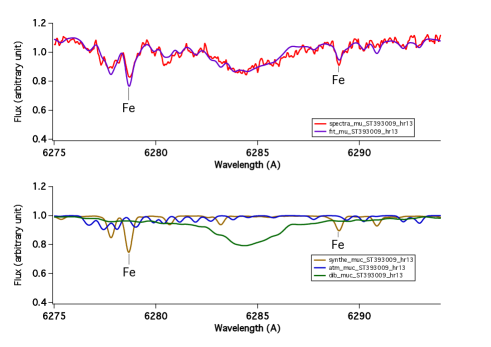
Figure 3: Model adjustment for Ogle N: 393009 (${T_{eff}}$ = 5012 K). The DIB is in a region devoid of strong stellar lines. The upper panel shows the spectrum (red line) and the best-fit model (purple line). The lower panel shows the synthetic stellar model (yellow line), the synthetic atmospheric model (blue line), and the DIB profile (green line) that all correspond to the fit parameters.

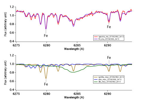
Figure 4: Same as Fig 3 for Ogle N: 392992 (${T_{eff}}$ = 4907 K). The DIB here is in a spectral region characterized by moderately strong stellar lines.

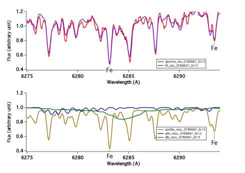
Figure 5: Same as Fig 3 for Ogle N: 89667 (${T_{eff}}$ = 4516 K). The DIB here is both weak and embedded in strong stellar lines.

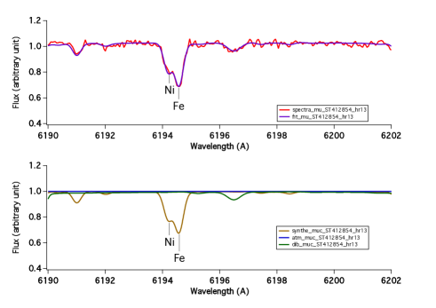
Figure 6: Same as Fig 3 for the 6196 Å DIB and Ogle N: 412854 (${T_{eff}}$ = 5191 K). The narrow DIB is in a region devoid of strong stellar lines.

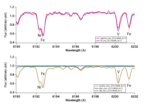
Figure 7: Same a Fig. 6 for Ogle N: 234898 (${T_{eff}}$ = 4714 K). The DIB and a strong stellar line do overlap.

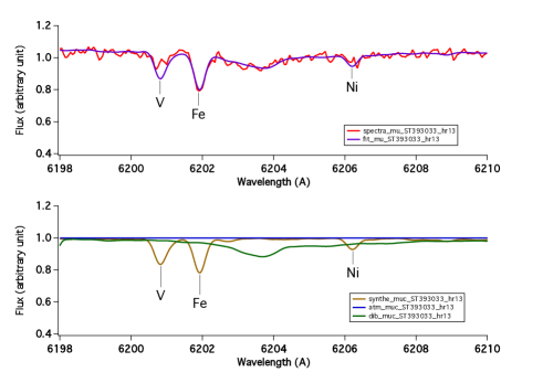
Figure 8: Same as Fig 3 for the 6204 Å  DIB and Ogle N: 393033 (${T_{eff}}$ = 4914 K). The narrow DIB is in a region devoid of strong stellar lines.

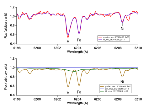
Figure 9: Same as Fig 8 for Ogle N: 268068 (${T_{eff}}$ = 4837 K). The DIB region corresponds to strong stellar line.

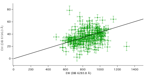
Figure 10: Equivalent width of DIB 6196.0 ${\AA}$ as a function of the equivalent width of DIB 6283.8 ${\AA}$. The black line is the best linear fit for pure proportionality, using error bars of both DIBs. The dotted line shows the linear fit with free offset.

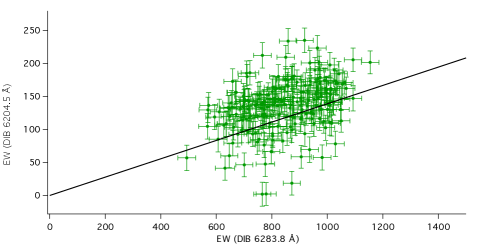
Figure 11: Same as figure 10 for DIB 6204 Å .

An immediate test of the reliability of the DIB strengths is the existence of DIB-DIB correlations, because EWs have been measured independently for the three bands. This test is is not so easy here due to the limited range of extinctions (Sumi, 2004). Still, the Spearman’s rank correlation statistics allows to reject the absence of two-by-two correlations by better than 99.9 %. Figures 10 and 11 show the DIBs 6196.0 and 6204.5 EWs as a function of the broad 6283.8 $\AA$ EW for the whole sample. The black lines correspond to a pure proportionality. Despite the existence of large uncertainties, especially for the two small DIBs, the correlation between the three bands is clearly visible. Those correlations show that the signal we extracted for the DIBs contains some information on the IS absorption, even for the two small DIBs. A second test of the DIB measurement is obtained from a comparison with the extinction map. Fig 12 displays the star-by-star variations of each DIB equivalent width as well as the extinction derived from the OGLE photometry obtained by interpolation through the Av map of Sumi (2004). The four patterns, that represent variations across the field of the four independent quantities, reveal large similarities for the strong DIB, some similarities for the 6204 Å DIB. Large uncertainties make the comparison less obvious for the 6196 Å band. This is reflected in the Spearman’s rank correlation statistics that allow to reject the absence of correlation at better than 99.9 % for the 6284 and 6204 DIBs, and 90 % for the 6196 Å DIB.

Better statistics could have been obtained after rejections of the noisy spectra or particularly poor adjustments. However, our goal here is to provide some idea of the DIB extraction results as a function of the signal quality, the DIB strength and the reddening for an entire field, with an entirely automated method.

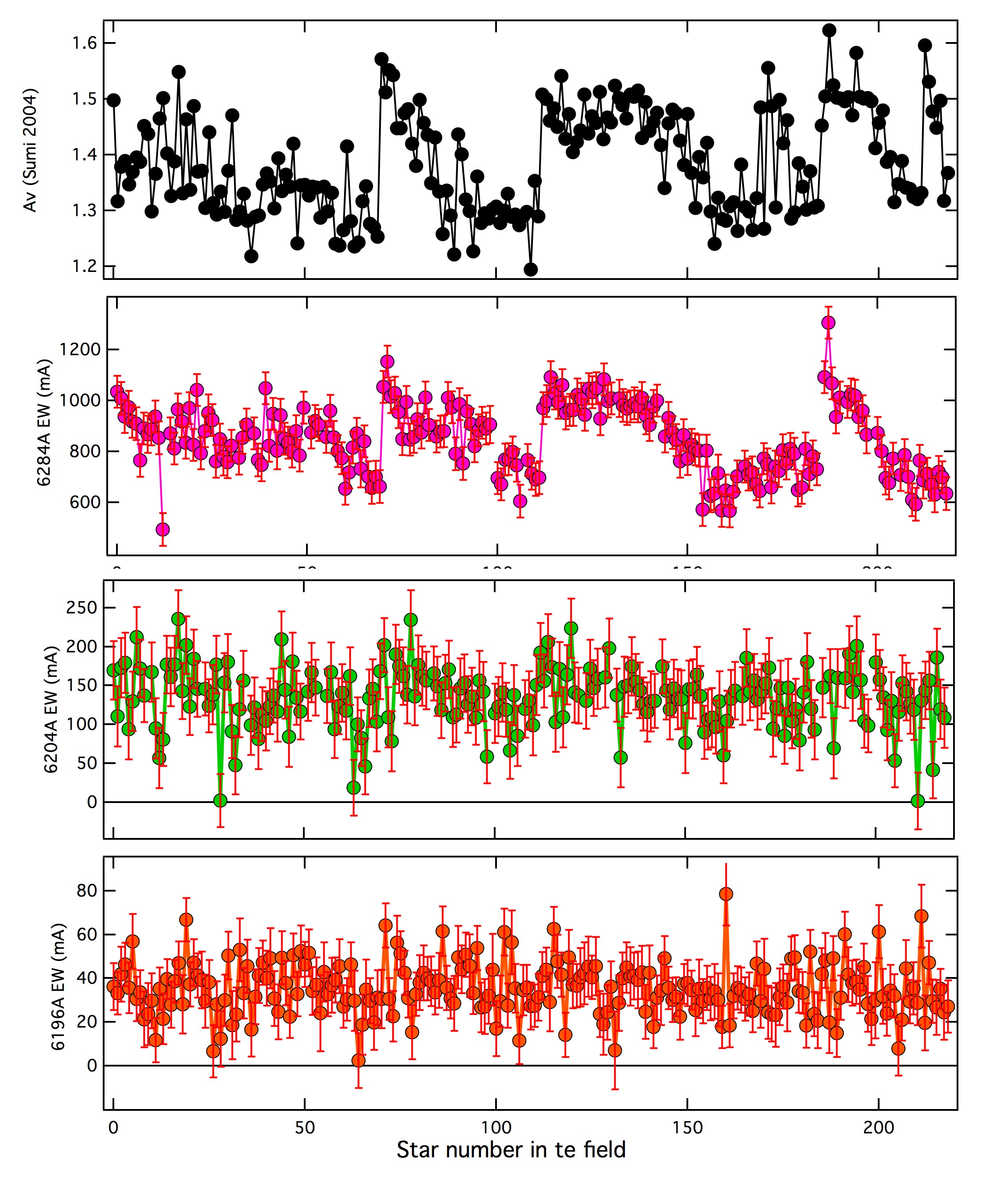
Figure 12: From bottom to top, equivalent widths of the three DIBs (6196, 6204 and 6284 Å ) as a function of the star number and the extinction Av interpolated from the map of Sumi (2004) at each star location.

6 Color excess estimates based on nearby star empirical relationships

DIBs are moderately or only weakly correlated with the extinction, as shown by a number of studies and the existence of DIB families whose members are internally closely correlated, while distinct families seem to obey different laws (e.g. Krelowski & Walker 1987, Cami et al. 1997). There is no parental link between the three DIBs we study here, and thus we do not expect to find strong correlations between their EWs nor very similar dependencies on the extinction. Previous surveys of stars in the solar neighborhood have provided some statistical relationships between the reddening E(B-V) derived from spectrophotometry and the equivalent width of each DIB. Best-fit parameters of linear correlations have been established recently by Friedman et al. (2011) for all three DIBs, based on about 130 O-B northern hemisphere nearby stars within 1 kpc. In the case of the 6284 Å DIBs, Raimond et al (2012) derived slightly different coefficients based on about the same number of southern hemisphere targets, observed with the ESO/La Silla FEROS spectrograph. Using the same FEROS data, Puspitarini and Lallement (2012) derived linear fit coefficients for the two other DIBs, again found slightly different when compared to the northern survey study. The coefficients for the linear relations between EW and $E_{B-V}$ are shown in Table 2 for both surveys and for the three DIBs. There are some differences between the relationships as they come out from the two surveys, that have been discussed by Raimond et al. (2012). Due to the use of cooler and fainter target stars, the ESO/FEROS DIB strengths are not as much influenced by strong radiation fields and there is significantly less dispersion around the mean DIB-E(B-V) relationship. As a matter of fact, DIB strengths may be significantly reduced in case the main dust cloud responsible for the absorption is very close to the UV-bright target star (Friedman et al. 2011, Vos et al. 2011), an effect attributed to the ionization state change of the carriers in the stellar environment. For this reason, the number of outliers with a relatively weak DIB and a large reddening is smaller in the FEROS survey, and the dispersion decreases. In parallel, the mean slope E(B-V)/EW(DIB) derived from the sample is also smaller. This was found systematically for the three DIBs. Here we will make use of the FEROS-based mean relationships, because the line-of-sight here is not related to hot bright stars and the DIB should in principle better correspond to average conditions. For comparisons we also show both results for the strong 6284 Å band.

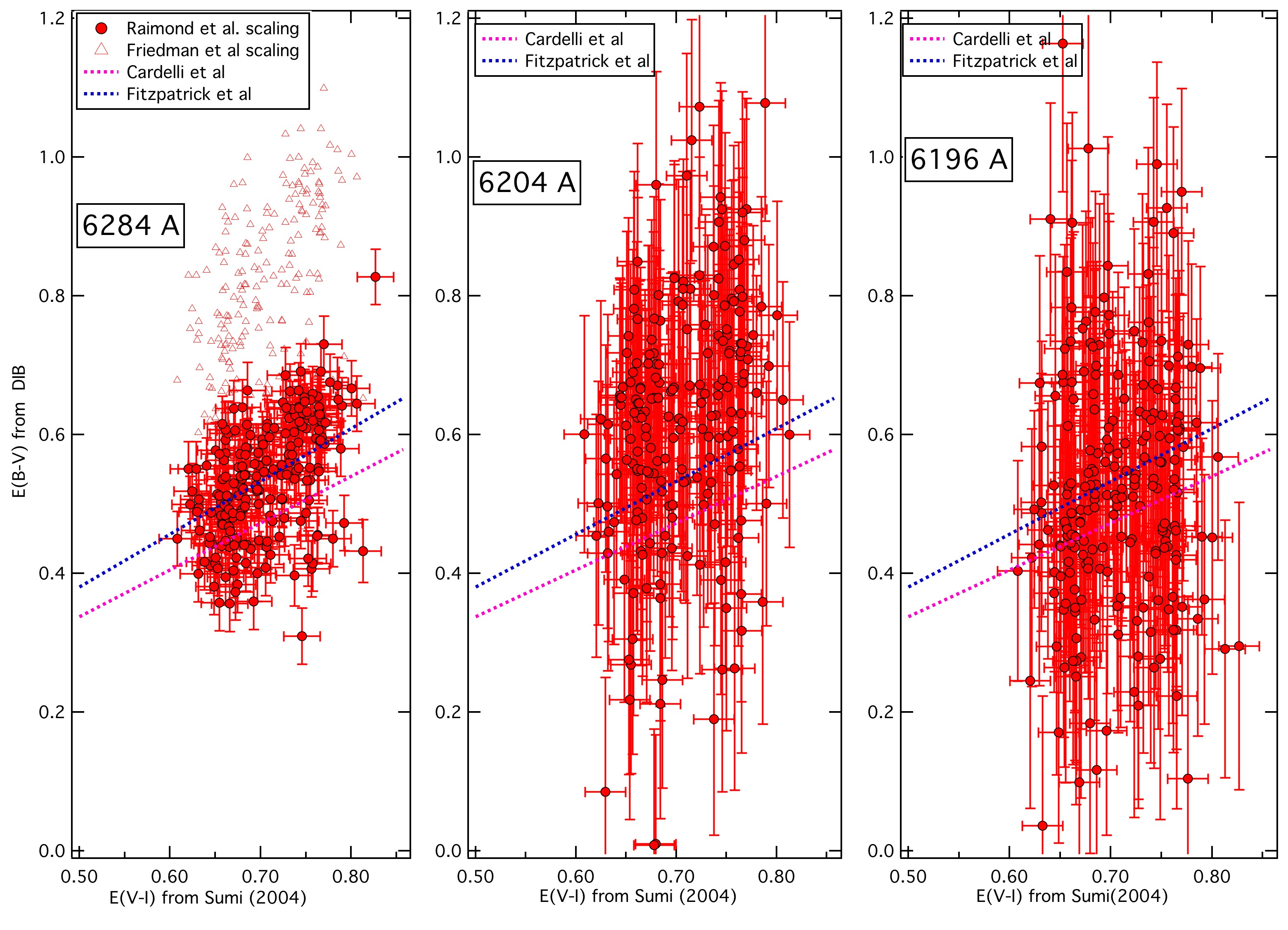
Figure 13: Color excess E(B-V) derived from the three DIBs as a function of the E(V-I) value interpolated within the Sumi (2004) map at the locations of the target stars. E(B-V)s here are obtained using the Raimond et al. (2012) and Puspitarini et al. (2012) average relationships based on FEROS data. The blue and pink dotted lines correspond to color excess relationships based on the Fitzpatrick (1999) and Cardelli et al. (1989) extinction curves and Rv=3.1 (see text). In the case of the DIBs 6283.8 ${\AA}$ we also show the color excess values deduced from the Friedman et al (2011) average relationships (open triangles).

The measured DIB equivalent widths derived from the global fitting were converted into $E_{B-V}$ color excess values by application of the three average relationships listed in Table 2.

Figure 13 shows the color excess $E_{B-V}$ estimate based on the DIB 6283.8 ${\AA}$ and the FEROS relationship, as a function of the color excess $E_{V-I}$ interpolated from the Sumi (2004) maps (x-axis). The figure is somewhat redundant with the previous one, however it provides a better idea of the equivalent width dispersion and the global relationship. The data point distribution shows a correlation between the DIB-based and photometric determinations, but there is a large dispersion, and also the observed interval for the DIB strength is significantly larger than the range of variation of the photometric determination (the best fit linear relationship does not go through zero). The relationship between $E_{B-V}$ and $E_{V-I}$ depends on the extinction curve, and in less extent on the stellar spectrum. We have drawn here the relationships based on both classical Cardelli et al. (1989) and Fitzpatrick (1999) extinction curves, for Rv= 3.1. E(V-I) is computed for a typical red-clump giant star, .and E(B-V) is computed for the A0 star Vega. As far as average absolute values are concerned, the DIB-based $E_{B-V}$s are similar to what one would expect from those classical laws, and in better agreement with the Fitzpatrick relationship. We also show the $E_{B-V}$ values we would obtain with the empirical Friedman et al (2011) relationship. Those $E_{B-V}$ empirical estimates are systematically higher and more difficult to reconcile with the photometric data. We believe that the relationship based on the cooler FEROS targets maybe more appropriate here because it probes environmental conditions that are closer to the average conditions encountered here than to the high ionization conditions encountered towards O- and early B-type nearby target stars.

Figure 13 also shows how the 6196 A and 6204 A DIB-based color excess $E_{B-V}$ compares with the photometric determination of $E_{V-I}$. For those two DIBs, the correlation is visible, and the agreement between the measured and the expected ratio between the two color excess values is again better with the Fitzpatrick et al. reddening law. There appears to be less deviation from average simple proportionality for those DIBs, compared to 6284Å , especially for the DIB 6196 for which the best-fit relationship is compatible with proportionality within the uncertainty range.

An important source of dispersion is the fact that the Sumi color excess is an average over the series of stars contained within the 0.6 x 0.6 arcmin pixel field and located at various distances in the bulge, while the DIB is derived for individual stars. Note that here the main effect would be angular variability, because, as said above, the quasi-totality of the extinction is generated closer than 2,000 pc, thus differences in the distances to the bulge targets have in principle no impact. At 1 kpc, 0.6 arcmin corresponds to a transverse distance of 0.17 pc, thus only very dense, small cloud cores could produce variations as large as those observed. A likely explanation for both the dispersion and also departures from proportionality between the DIB-based color excess and the photometric E(V-I) is the existence of intrinsic DIB variations in response to the radiation field and in general to environmental conditions, such like those found at smaller distances. This is favored by the spatial pattern as we will discussed below. On the other hand, spatial variations of the DIB-E(V-I) ratio may also be related to spatial variability of the extinction curve. Udalski (2003) and Sumi (2004) both consider that towards the bulge Rv may vary significantly. A relationship between the extinction curve, the total to selective extinction ratio and the DIB behavior has been first discussed by Krelowski et al (1999). Environmental effects and dust processing on one hand, and extinction curve on the other hand are themselves related through the grain distribution and the cloud history, which also influences DIB carriers and strengths.

The spatial variability of the ratio between DIB-based and photometric determinations of the color excess is shown superimposed on the Sumi map in Figure 14. In this figure the color indicates the ratio and the size of the markers is proportional to the DIB strength. The distribution of colors shows that there are some systematic changes across the field for the 6284 DIB, in particular the DIB is relatively small compared to the photometric value at larger declinations and right ascensions. Future investigations will hopefully allow to attribute or not those differences to variations of the environmental conditions in the encountered clouds, or to extinction law spatial variations, or both, as discussed above. The 6204 Å DIB shows the same behavior than the 6284 band, although less clearly due to large uncertainties and also not so pronounced. At variance with the two other bands, the 6196 Å DIB does not reveal any spatial trend, although there are strong uncertainties on the DIB equivalent width. If confirmed, for the three DIBS the spatial homogeneity of the measured ratio follows the degree of correlation of the DIBs with the color excess, as measured in the solar neighborhood and for widely distributed targets by Friedman et al (2011). The correlation degree and spatial homogeneity decrease from the 6284 Å DIB to the small 6196 Å DIB .

Finally, we show in Figure 15 a weighted mean value of $E_{B-V}$ derived from the three DIBs, again compared with the $E_{V-I}$ value deduced from the OGLE analysis. This figure allows to figure out to which extent the combination of those three DIBS can be used here as a first estimator for the reddening, in the absence of photometric measurements. The average linear relationship is $E_{B-V}$= (0.72 $\pm$ 0.14) $E_{V-I}$ + (0.06 $\pm$0.10) and the standard deviation is 0.08, i.e. of the order of 15% of the average value. This should be compared with other conditions and distances.

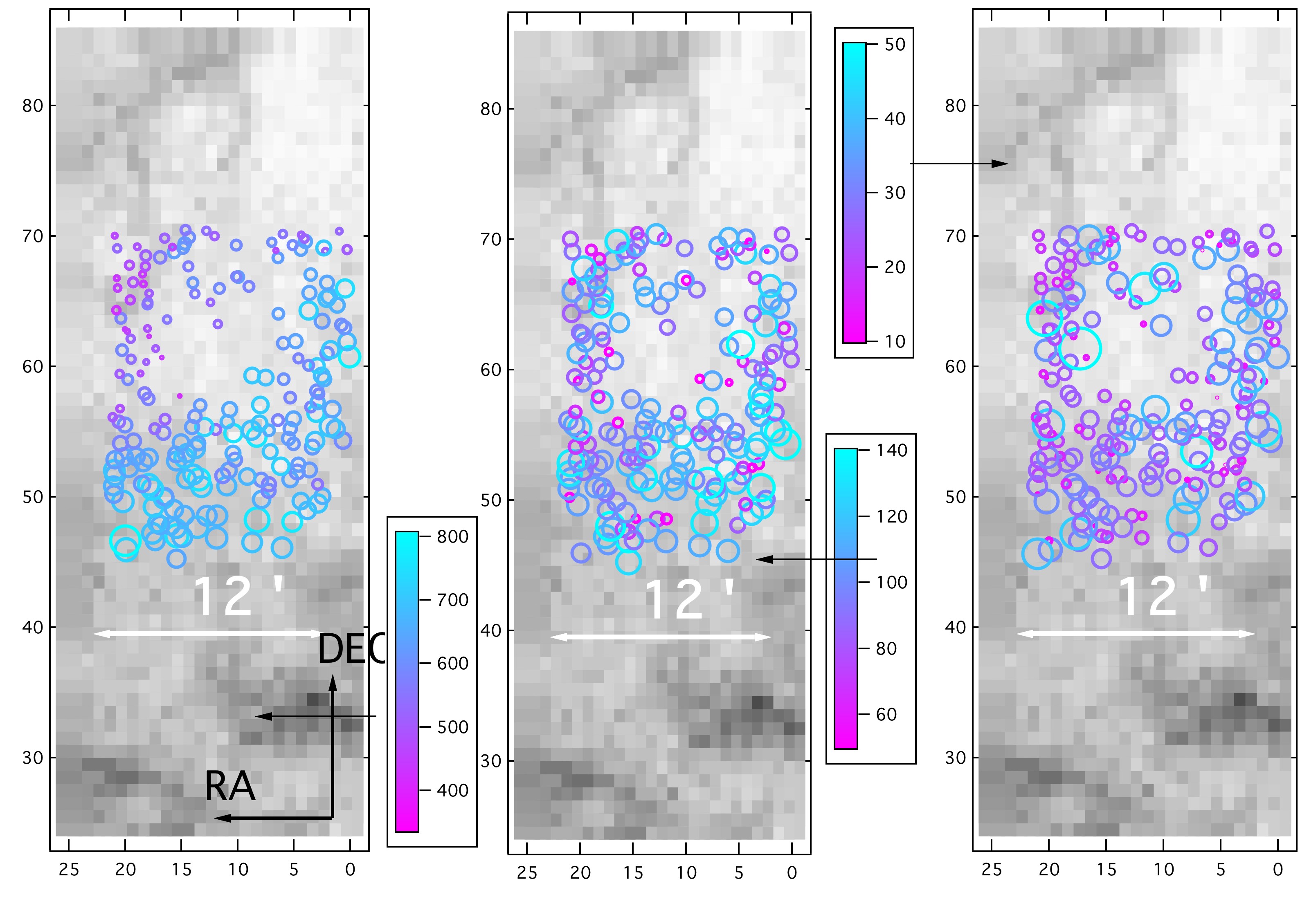
Figure 14: Spatial variability of the DIB and the DIB-extinction ratio (from left to right, the 6284, 6204, 6196 Å DIBs). Target stars used in this study are superimposed on the Av extinction map from Sumi (2004) (grey scale). The size of the circle is proportional to the DIB equivalent width, and its color corresponds to the ratio between the DIB equivalent width and the extinction Av obtained by interpolation through the Sumi map (color scale).

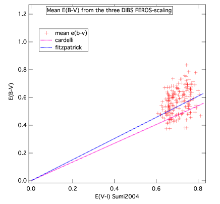
Figure 15: A synthesis of all E(B-V)s estimates from the 3 DIBs, under the form of a weighted mean, here compared with the E(V-I) determination from the OGLE photometry. The blue and pink dotted lines correspond to color excess relationships based on the Fitzpatrick et al. and Cardelli et al. extinction curves.

Table 2: E(B-V)_λ=a+b*EW_λ. Reference 1: Friedman et al. Friedman et al. (2011); 2: Puspitarini and Lallement (2012); 3: Raimond et al. Raimond et al. (2012).

DIBλ	Reference	a	b
6196.0	1	(-5.07$\pm$0.56)*$10^{-2}$	(2.11$\pm$0.02)*$10^{-2}$
	2	0	(1.48$\pm$0.09)*$10^{-2}$
6204.5	1	(-7.22$\pm$0.67)*$10^{-2}$	(5.99$\pm$0.08)*$10^{-3}$
	2	0	(4.58$\pm$0.37)*$10^{-3}$
6283.8	1	(-7.71$\pm$0.78)*$10^{-2}$	(9.57$\pm$0.17)*$10^{-4}$
	3	(-0.50$\pm$0.40)*$10^{-2}$	(6.37$\pm$0.23)*$10^{-4}$

7 Summary and discussion

We have used R=22,500, S/N= 30-77 observations of 219 red clump giants from the galactic bulge in the Baade’s Window (Av $\simeq$ 1.4) as a test case of our newly developed composite model and automated fitting method of interstellar absorption extraction from cool star spectra. The combination of synthetic stellar models, synthetic atmospheric lines, and DIB profiles allowed to extract equivalent width values for the three 6284, 6196 and 6204 Å  DIBs. The existence of DIB-DIB correlations demonstrates that, even without any adaptation of the stellar model, in the case of a moderate color excess E(B-V) $\simeq$ 0.4 and signal to noise ratios above 30, a strong DIB like the 6284 Å  band but also narrow and weaker DIBs like the 6196 or the 6204 Å bands can be measured for cool stars, provided one takes into account the velocity shift between the star and the absorbing ISM. More precisely, all spectra could be efficiently used in the case of the strong and broad 6284 $\AA$ DIB (width $\simeq$ 3.5 Å  depth $\simeq$ 20%), while for the two narrow and weaker DIBs ($\simeq$ 0.5 and 1 Å width, 10 % depth) the potential extraction of the DIB equivalent width depends on the star’s radial velocity, whose value results or not in an overlap of stellar lines and DIBs. This is due to the presence of unidentified lines as well as over- or under-predicted line strengths. Model improvements are beyond the scope of this work, but should be performed in future, once other analyses confirm the present trends and enough constraints are obtained. Here we simply performed an empirical correction, independently for each DIB, that is described in the Appendix. Its validity was demonstrated by a strong improvement of the DIB-DIB correlations as well as improvements of the DIB-extinction correlations. More work is needed on a more fundamental approach to those corrections. Globally, this modeling demonstrates that DIBs can be measured in an automated way for large number of cool targets during spectroscopic surveys, and be used as any other IS line to locate the IS matter.

For the three DIBs the spatial pattern globally reflects extinction variations deduced from stellar photometry, which also validates the fitting method. The degree of correlation is, as expected, globally better for the broader and stronger DIB because uncertainties on the equivalent widths are much smaller. DIB strengths are converted into color excesses, using best-fit linear relationships established for early-type star surveys. Mean values of E(B-V) over all targets are 0.53, 0.62 and 0.52 for the 6284, 6204, and 6196 Å DIBs respectively. Discrepancies among the DIBS amount to about 20%, and there is a 15% dispersion of the weighted mean value around its average linear relationship with the photometric reddening (Fig. 15). Several results were obtained from the analysis, that call for further studies. The 6284, and in a smaller extent the 6204 Å DIBs amplitude intervals over the field are found to be larger than the color excess relative variations deduced from OGLE photometric data and their analysis (Sumi 2004, see Fig 12). This is reflected in a spatial variability of the DIB-based to photometry-based color excess ratio. Those variations are not randomly located, as is especially visible for the 6284 Å DIB: the DIB is systematically weaker around $\alpha,\delta$ = 270.95,-30 ^∘. One likely explanation for such departures from proportionality is the DIB response to ionization conditions in the clouds, and other environmental effects such like shocks.This may be linked to a spatial variability of the extinction law. The grain size distribution influences the shape of the extinction law and he total to selective extinction ratio, but is also linked to the cloud physical properties and its history, that themselves influence the quantity of macro-molecules and the DIBs. Such a link between the total to selective extinction ratio and the DIBs has been discussed by Krelowski et al. (1999). The excess of amplitude variation and the spatial variability do not seem to exist for the small 6196 Å  DIB, although large uncertainties make the comparison with the photometric extinction more difficult. This may be put in relation with the fact that this DIB has been found to be better correlated with the extinction than the two others, something again potentially related to its different response to the dust distribution, or the environmental conditions. Moreover, the absolute value of the extinction based on the 6196 Å DIB (again deduced from the average solar neighborhood relationship) seems to agree better with the photometric determination as compared with the two other DIBs.

More analyses should be performed over various fields and for targets at various distances to confirm unidentified or poorly predicted stellar lines. More data should help refining the stellar models in the DIB spectral regions and subsequently improving the DIB extraction. On the other hand, extinction estimates would certainly be strongly improved by the use of multiple DIBs and of their ratios, accompanied by a better understanding of their specific behavior. Such studies may also provide additional information on the links between the extinction law and the DIBs.

Table 3: Stellar data and measurement of EW

Star	OgleN	Teff	log $g$	$\xi$	[Fe/H]	$E_{B-V}*$	EW(6196)	corr’d	EW6204)	corr’d	EW6284	corr’d
		K	dec	kms-1	dec		m${\AA}$	m${\AA}$	m${\AA}$	m${\AA}$	m${\AA}$	m${\AA}$
1	67536	5121	2.43	1.1	-0.45	0.483	40	36$\pm$11	164	170$\pm$38	1046	1036$\pm$62
2	67610	4865	2.34	1.5	-0.31	0.425	36	33$\pm$10	110	111$\pm$38	1053	1009$\pm$64
3	67641	4575	2.17	1.4	-0.36	0.445	50	42$\pm$13	164	173$\pm$38	962	939$\pm$64
4	67663	4878	2.33	1.4	-0.05	0.448	50	46$\pm$10	175	179$\pm$39	1023	974$\pm$64
5	67675	4507	2.16	1.5	0.42	0.434	49	36$\pm$12	87	94$\pm$38	991	919$\pm$64
6	67687	4664	2.27	1.5	0.54	0.442	64	57$\pm$13	130	130$\pm$38	942	909$\pm$64
7	67727	4994	2.45	1.5	0.55	0.45	37	31$\pm$10	206	213$\pm$38	838	766$\pm$64
8	67744	5170	2.42	1.4	-0.43	0.447	36	34$\pm$10	175	172$\pm$37	895	891$\pm$62
9	67762	4943	2.34	1.3	-0.26	0.468	21	21$\pm$13	131	137$\pm$34	884	868$\pm$73
10	78185	4763	2.3	1.2	0.21	0.464	13	24$\pm$14	105		840	887$\pm$62
11	78195	4807	2.34	1.1	-0.05	0.419	34	30$\pm$13	161	167$\pm$38	951	938$\pm$62
12	78202	4460	2.17	1.5	0.54	0.441	19	12$\pm$10	88	95$\pm$38	924	855$\pm$64
13	78205	5271	2.37	1	0.2	0.473	39	35$\pm$10	53	57$\pm$38	555	493$\pm$64
14	78215	4738	2.22	1.6	0.55	0.484	38	22$\pm$12	53	81$\pm$34	747
15	78255	4810	2.31	1.4	0.49	0.452	38	40$\pm$9	184	177$\pm$37	852	871$\pm$63
16	78271	4685	2.21	1.5	0.17	0.428	24	28$\pm$11	155	161$\pm$38	816	813$\pm$62
17	78281	4899	2.31	1.1	0.2	0.448	32	39$\pm$10	179	177$\pm$37	945	966$\pm$63
18	78283	4512	2.21	1.5	0.35	0.5	48	47$\pm$10	242	235$\pm$37	895	918$\pm$63
19	78288	5136	2.3	1.5	-0.48	0.429	27	28$\pm$13	126	143$\pm$36	800	835$\pm$63
20	78322	4978	2.37	0.8	-0.67	0.472	70	67$\pm$10	205	202$\pm$37	978	970$\pm$63
21	78323	4867	2.35	1.5	0.3	0.431	27	37$\pm$10	131	123$\pm$36	799	827$\pm$63
22	78330	4595	2.18	1.5	0.61	0.48	40	47$\pm$11	180	185$\pm$37	1035	1042$\pm$62
23	78354	4738	2.29	1	0.03	0.442	35	41$\pm$10	152	146$\pm$36	768	793$\pm$63
24	78357	4620	2.09	1.5	0.37	0.442	29	39$\pm$13	136		840	880$\pm$63
25	78379	4775	2.31	1.3	0.03	0.421	34	30$\pm$12	131	146$\pm$34	960	952$\pm$73
26	78393	4943	2.26	1.2	-0.18	0.465	33	38$\pm$10	133	124$\pm$34	903	924$\pm$63
27	78401	4851	2.24	1.5	0.14	0.424	11	7$\pm$12	140	138$\pm$38	818	762$\pm$64
28	78421	4632	2.22	1.5	0.46	0.417	25	28$\pm$11	177	177$\pm$37	838	849$\pm$62
29	78436	4541	2.19	1.3	0.32	0.43	23	12$\pm$13	-21	2$\pm$34	802	780$\pm$73
30	78449	4947	2.22	1.7	0.54	0.418	25	30$\pm$12	155	154$\pm$38	759	758$\pm$62
31	78461	4539	2.16	1.3	0.32	0.442	37	50$\pm$11	218	180$\pm$36	809	824$\pm$63
32	89573	4819	2.25	1.4	0.35	0.474	44	19$\pm$16	74	91$\pm$34	885
33	89589	4690	2.13	1.5	-0.13	0.414	25	24$\pm$12	48	48$\pm$38	817	777$\pm$67
34	89590	5151	2.42	1.5	-0.23	0.419	37	53$\pm$14	115	120$\pm$36	798	854$\pm$62
35	89609	4898	2.29	1.2	-0.15	0.429	35	33$\pm$12	149	157$\pm$38	915	906$\pm$62
36	89614	4734	2.26	1.5	0.59	0.414	39	46$\pm$12	76		784
37	89640	4641	2.21	1.5	0.19	0.393	18	17$\pm$12	97	99$\pm$38	878	872$\pm$62
38	89645	4674	2.22	1.6	0.28	0.416	41	32$\pm$13	118	122$\pm$38	797	767$\pm$64
39	89667	4516	2.11	1.5	0.66	0.417	53	41$\pm$13	78	81$\pm$38	783	748$\pm$64
40	89669	4964	2.44	1.4	0.39	0.434	35	47$\pm$10	141	113$\pm$34	1029	1050$\pm$63
41	89687	4743	2.33	1.5	0.5	0.441	43	40$\pm$13	106	105$\pm$38	846	822$\pm$63
42	89702	4714	2.2	1.2	0.2	0.436	31	49$\pm$14	148	124$\pm$36	913	949$\pm$62
43	89731	4784	2.22	1.3	-0.12	0.421	33	31$\pm$13	129	137$\pm$35	825	803$\pm$72
44	89735	4579	2.07	1	0.11	0.45	36	25$\pm$13	111	116$\pm$38	976	944$\pm$64
45	89736	4483	2.15	1.4	0.47	0.431	30	50$\pm$12	255	210$\pm$36	837	850$\pm$63
46	89774	4635	2.13	1.5	0.22	0.44	39	38$\pm$10	150	145$\pm$37	820	834$\pm$62
47	89786	4705	2.31	1.1	-0.19	0.433	26	23$\pm$10	82	84$\pm$39	851	803$\pm$64
48	89802	4481	2.12	1.5	0.45	0.458	52	51$\pm$10	188	181$\pm$37	855	881$\pm$62
49	89832	4546	2.14	1.4	0.17	0.4	25	33$\pm$10	150	134$\pm$35	757	785$\pm$63
50	89843	5270	2.38	1.1	0.17	0.434	40	53$\pm$12	144	116$\pm$36	956	972$\pm$63
51	89848	4582	2.08	1.4	0.09	0.434	47	46$\pm$10	72		931
52	89871	4502	2.17	1.5	0.36	0.428	47	52$\pm$11	138	142$\pm$37	872	876$\pm$62
53	101453	4966	2.39	1.2	-0.1	0.433	35	34$\pm$11	160	167$\pm$38	928	920$\pm$62
54	101462	4807	2.25	1.3	0.07	0.433	24	37$\pm$13	167	147$\pm$36	883	904$\pm$63
55	101470	4567	2.2	1.4	0.62	0.415	5	24$\pm$17	22		999
56	101476	4838	2.34	1.5	-0.11	0.433	30	43$\pm$14	110		802	858$\pm$63
57	101486	4760	2.15	1.3	-0.6	0.419	34	33$\pm$10	135	136$\pm$35	941	961$\pm$63
58	101505	4584	2.16	1.5	0.17	0.429	44	37$\pm$13	164	168$\pm$38	884	856$\pm$64
59	101540	4754	2.35	1.5	0.38	0.4	39	39$\pm$10	98	94$\pm$37	789	803$\pm$62
60	101606	4647	2.08	1.5	0.58	0.399	23	46$\pm$12	175	123$\pm$36	763	775$\pm$63
61	101638	4556	2.14	1.4	-0.37	0.408	28	27$\pm$10	145	140$\pm$37	650	654$\pm$63
62	101648	5025	2.33	1.6	-0.07	0.457	31	30$\pm$10	124	118$\pm$37	708	719$\pm$63
63	101650	4801	2.21	1.5	0.44	0.413	48	46$\pm$10	169	162$\pm$37	792	815$\pm$62
64	101655	5274	2.46	1.2	0.71	0.399	14	30$\pm$14	76	19$\pm$36	826	872$\pm$62
65	101662	4465	2.05	1.2	0.29	0.401	12	3$\pm$13	80	100$\pm$35	757	733$\pm$73
66	101674	4644	2.23	1.5	0.43	0.425	-5	19$\pm$14	122	83$\pm$36	808	840$\pm$62
67	101681	4763	2.23	1.5	0.36	0.433	22	35$\pm$14	82	46$\pm$36	654	701$\pm$62
68	101691	4857	2.23	1.6	0.21	0.412	30	30$\pm$10	137	134$\pm$37	649	658$\pm$62
69	101692	4449	1.99	1.5	0.25	0.41	21	20$\pm$12	145	146$\pm$38	707	702$\pm$62
70	101703	4931	2.2	1.5	0.16	0.404	41	31$\pm$13	99	103$\pm$38	691	662$\pm$64
71	234759	4458	2.06	1.5	0.35	0.507	6	31$\pm$13	204	169$\pm$36	1028	1055$\pm$63
72	234802	4288	1.97	0.8	0.23	0.488	55	64$\pm$10	229	202$\pm$35	1135	1154$\pm$63
73	234810	4521	2.12	1.2	-0.5	0.5	32	31$\pm$10	111	109$\pm$39	1054	1016$\pm$64
74	234811	4773	2.28	1.4	-0.39	0.498	24	23$\pm$11	81	78$\pm$39	1075	1029$\pm$64
75	234849	4556	2.19	1.2	0.2	0.467	57	56$\pm$12	188	190$\pm$38	961	956$\pm$62
76	234877	4538	2.14	0.8	-0.2	0.467	47	52$\pm$10	183	175$\pm$34	828	849$\pm$63
77	234898	4714	2.26	0.8	0.18	0.476	44	42$\pm$10	167	162$\pm$37	984	995$\pm$62
78	234905	5042	2.28	1.3	-0.12	0.478	30	31$\pm$9	143	138$\pm$37	836	847$\pm$63
79	234917	5050	2.39	1.5	-0.7	0.458	24	16$\pm$12	217	234$\pm$38	874	859$\pm$62
80	234926	4830	2.3	1.3	-0.68	0.445	36	33$\pm$10	140	136$\pm$37	934	928$\pm$63
81	234929	4893	2.35	0.8	-0.68	0.483	47	38$\pm$13	161	177$\pm$38	892	874$\pm$62
82	235017	4798	2.31	1.4	0	0.47	47	43$\pm$13	156	162$\pm$38	1024	1012$\pm$62
83	244618	4410	2.03	1.4	-0.17	0.463	42	40$\pm$10	161	157$\pm$37	899	905$\pm$63
84	244635	4650	2.24	1.5	-0.19	0.435	35	39$\pm$11	119		855
85	244642	4757	2.15	1.5	0.3	0.462	24	34$\pm$10	185	166$\pm$35	830	859$\pm$63
86	244660	4736	2.17	1.3	-0.28	0.43	44	39$\pm$13	139	149$\pm$38	890	878$\pm$62
87	244668	4627	2.17	1.5	0.51	0.406	44	62$\pm$11	167	119$\pm$36	868	880$\pm$63
88	244704	4916	2.22	1.3	-0.14	0.431	31	36$\pm$10	156	153$\pm$36	989	1012$\pm$63
89	244718	4724	2.29	1.4	0.12	0.417	30	31$\pm$9	177	171$\pm$37	960	974$\pm$63
90	244727	4641	2.27	1.3	0.35	0.394	36	29$\pm$13	107	109$\pm$38	823	792$\pm$64
91	244728	4491	2.03	1.5	0.3	0.463	39	50$\pm$14	140	112$\pm$36	940	987$\pm$62
92	244734	4900	2.26	1.5	0.52	0.452	52	44$\pm$11	140	147$\pm$39	811	754$\pm$64
93	244742	4735	2.23	1.5	-0.03	0.426	53	51$\pm$10	158	153$\pm$37	952	959$\pm$62
94	244757	4910	2.23	1.2	-0.53	0.419	29	46$\pm$14	107	126$\pm$36	857	908$\pm$62
95	244763	4775	2.19	1.5	0.14	0.396	33	33$\pm$10	143	136$\pm$37	806	822$\pm$63
96	244817	4610	2.11	1.5	0.57	0.439	40	54$\pm$10	149	109$\pm$35	866	884$\pm$63
97	244840	4605	2.11	1.5	0.45	0.412	21	27$\pm$11	156	157$\pm$38	916	914$\pm$62
98	256395	4650	2.21	1.6	0.41	0.418	27	27$\pm$13	143	142$\pm$38	896	892$\pm$62
99	256401	4650	2.29	1.5	0.54	0.415	47	32$\pm$13	28	59$\pm$34	931	906$\pm$73
100	256570	4843	2.19	1.5	0.56	0.42	32	44$\pm$16	97		681
101	256579	4737	2.26	1.5	0.36	0.422	17	17$\pm$12	115	114$\pm$38	699	695$\pm$62
102	256650	4598	2.19	1.5	0.44	0.412	26	30$\pm$12	124	123$\pm$38	674	672$\pm$62
103	267856	4605	2.2	1.2	0.04	0.419	60	61$\pm$11	137	141$\pm$37	771	769$\pm$62
104	267862	4686	2.23	1.1	-0.17	0.429	23	28$\pm$10	127	119$\pm$35	747	771$\pm$63
105	267909	4716	2.16	1.4	0.43	0.416	46	56$\pm$14	105	67$\pm$36	750	798$\pm$62
106	267912	4781	2.28	1.5	0.38	0.417	44	36$\pm$11	132	138$\pm$38	797	746$\pm$64
107	267985	4990	2.23	1.4	-0.14	0.411	16	12$\pm$11	85	85$\pm$39	660	606$\pm$64
108	268000	4568	2.2	1.5	0.19	0.416	31	35$\pm$12	29		740
109	268011	4696	2.24	1.7	0.4	0.419	36	36$\pm$10	126	120$\pm$37	751	767$\pm$62
110	268022	4968	2.26	1.5	0.22	0.385	24	27$\pm$11	128	131$\pm$37	712	714$\pm$62
111	268047	4880	2.34	1.3	0.09	0.437	31	28$\pm$10	96	99$\pm$38	749	691$\pm$64
112	268068	4837	2.31	1.7	0.3	0.416	39	31$\pm$11	144	151$\pm$39	767	698$\pm$64
113	385048	4686	2.24	1.2	-0.36	0.486	45	41$\pm$11	183	192$\pm$38	982	971$\pm$62
114	392992	4907	2.34	1.2	-0.22	0.484	40	44$\pm$10	163	156$\pm$34	977	998$\pm$63
115	393009	5012	2.32	1.5	-0.68	0.471	33	29$\pm$13	176	206$\pm$36	1054	1093$\pm$63
116	393012	4540	2.24	1.5	0.48	0.478	64	63$\pm$10	181	174$\pm$37	1006	1028$\pm$62
117	393024	4786	2.26	1.2	-1.13	0.468	35	48$\pm$12	112	103$\pm$38	1018	994$\pm$65
118	393026	4804	2.3	1.2	-0.5	0.497	41	42$\pm$10	168	171$\pm$35	1039	1061$\pm$63
119	393028	4457	2.13	1.4	0.36	0.461	18	14$\pm$10	103	109$\pm$39	1011	952$\pm$64
120	393030	4574	2.18	1.5	0.35	0.475	53	50$\pm$13	163	164$\pm$38	987	964$\pm$63
121	393033	4914	2.32	1	-0.5	0.453	43	37$\pm$11	213	224$\pm$38	976	964$\pm$62
122	393070	4903	2.3	1.6	0.47	0.459	41	37$\pm$10	134	141$\pm$38	1087	1023$\pm$64
123	393088	4575	2.21	1.5	0.22	0.466	20	41$\pm$13	164	137$\pm$36	979	1007$\pm$63
124	393091	4641	2.15	1.5	0.47	0.486	34	42$\pm$14	142		904	944$\pm$62
125	393111	4546	2.21	1.5	0.23	0.464	31	45$\pm$14	157	130$\pm$36	1005	1048$\pm$62
126	393117	4931	2.26	0.9	-0.07	0.474	36	40$\pm$10	173	172$\pm$37	1015	1033$\pm$63
127	393124	4540	2.08	1.5	0.5	0.47	17	46$\pm$13	192	147$\pm$36	1025	1050$\pm$63
128	393125	4528	2.09	1.4	0.29	0.488	30	24$\pm$11	153	159$\pm$39	982	929$\pm$64
129	393136	4515	2.11	1.4	0.5	0.461	10	19$\pm$14	152		1047	1085$\pm$63
130	393138	5073	2.34	1.4	-0.64	0.473	33	24$\pm$13	153	161$\pm$38	1020	999$\pm$64
131	393152	4757	2.23	1.3	-0.2	0.47	39	36$\pm$12	189	198$\pm$38	1019	1009$\pm$62
132	393162	4359	2.05	1.5	0.39	0.492	-15	7$\pm$18	161		953
133	393229	4868	2.32	1.3	-0.59	0.485	21	29$\pm$13	144	138$\pm$34	1021	1010$\pm$73
134	393319	4473	2.19	1.4	0.26	0.48	50	40$\pm$12	55	58$\pm$38	1045	981$\pm$64
135	393339	4972	2.41	1	-0.09	0.473	53	45$\pm$12	143	148$\pm$38	1007	968$\pm$64
136	402417	4655	2.2	1.2	-0.2	0.486	32	41$\pm$13	151	150$\pm$36	945	978$\pm$63
137	402421	4822	2.36	1.3	0.19	0.485	37	41$\pm$11	169	174$\pm$38	990	990$\pm$62
138	402432	4579	2.12	1.5	0.29	0.489	19	39$\pm$13	187	155$\pm$36	951	977$\pm$63
139	402433	4808	2.24	1.3	-0.19	0.461	36	43$\pm$12	149	144$\pm$36	989	1010$\pm$63
140	402435	4618	2.25	1.2	0	0.482	29	25$\pm$12	112	127$\pm$34	951	942$\pm$73
141	402440	4429	2.11	1.3	0.29	0.465	45	43$\pm$13	115	116$\pm$38	912	904$\pm$62
142	402449	4474	2.18	1.5	0.26	0.471	23	18$\pm$10	125	130$\pm$38	1042	978$\pm$64
143	402463	5260	2.43	1.2	-0.51	0.476	30	31$\pm$10	128	131$\pm$35	979	1001$\pm$63
144	402470	4270	1.97	1.2	0.16	0.457	27	35$\pm$16	111		902
145	402477	4545	2.19	1.5	0.51	0.432	37	49$\pm$10	196	175$\pm$35	827	859$\pm$63
146	402478	4983	2.35	1.2	-0.53	0.47	36	36$\pm$10	143	143$\pm$37	917	932$\pm$63
147	402482	4871	2.28	1.3	-0.57	0.478	34	30$\pm$10	118	120$\pm$39	910	875$\pm$64
148	402502	4818	2.19	1.2	-0.95	0.476	32	32$\pm$9	146	146$\pm$37	840	846$\pm$63
149	402516	4936	2.2	1.3	-0.65	0.46	27	22$\pm$10	130	133$\pm$39	791	761$\pm$64
150	402518	5034	2.32	1	-0.87	0.446	39	37$\pm$9	133	133$\pm$37	858	865$\pm$63
151	402550	4420	2.15	1.5	0.39	0.475	46	38$\pm$11	69	76$\pm$39	845	772$\pm$64
152	402560	4984	2.37	1.1	-1.01	0.441	35	35$\pm$9	146	145$\pm$37	825	826$\pm$63
153	402600	5158	2.4	1.3	-0.52	0.421	32	25$\pm$12	132	146$\pm$38	823	810$\pm$62
154	402621	4913	2.28	1.3	-0.56	0.45	37	35$\pm$13	142	164$\pm$36	767	804$\pm$63
155	402632	4937	2.32	1.5	0.55	0.439	34	30$\pm$10	130	137$\pm$39	635	572$\pm$64
156	402641	4775	2.18	1.5	0.49	0.458	23	36$\pm$10	120	90$\pm$34	782	803$\pm$63
157	412854	5191	2.4	1.4	-0.69	0.419	34	31$\pm$10	105	107$\pm$39	658	627$\pm$64
158	412889	4717	2.23	1.6	0.42	0.4	39	34$\pm$13	108	108$\pm$38	665	635$\pm$64
159	412894	5118	2.31	1.5	-0.45	0.427	25	30$\pm$12	99	97$\pm$34	724	715$\pm$73
160	412898	4871	2.22	1.8	0.07	0.415	22	18$\pm$10	126	130$\pm$38	627	570$\pm$64
161	412921	4617	2.13	1.5	0.47	0.413	69	79$\pm$14	99	60$\pm$36	601	647$\pm$62
162	412957	4920	2.23	1.5	-0.54	0.422	21	19$\pm$10	105	105$\pm$39	604	568$\pm$64
163	412979	4756	2.24	1.5	-0.58	0.424	36	32$\pm$10	134	133$\pm$37	652	643$\pm$62
164	413012	4869	2.29	1.2	-0.15	0.408	32	36$\pm$10	144	143$\pm$37	685	704$\pm$63
165	413043	4974	2.24	1.5	0.09	0.446	34	35$\pm$10	83		699
166	413060	4811	2.29	1.1	-0.37	0.422	29	31$\pm$10	136	136$\pm$37	724	741$\pm$63
167	413066	4674	2.11	1.5	0.44	0.419	33	33$\pm$10	193	186$\pm$37	684	709$\pm$63
168	423393	4702	2.28	1.5	0.41	0.408	24	25$\pm$10	150	143$\pm$37	696	718$\pm$63
169	423398	4351	2.05	1.3	0.42	0.426	35	47$\pm$10	182	156$\pm$34	646	672$\pm$63
170	423427	4818	2.22	1.5	0.33	0.479	41	30$\pm$12	126	132$\pm$38	688	646$\pm$64
171	423432	4945	2.36	1.4	-0.55	0.409	36	44$\pm$14	119	143$\pm$36	727	773$\pm$62
172	423434	4753	2.31	1.5	-0.15	0.502	28	25$\pm$12	145	153$\pm$38	759	749$\pm$62
173	423461	4743	2.24	1	-0.13	0.48	27	24$\pm$12	165	173$\pm$38	668	659$\pm$62
174	423485	4779	2.3	1.5	0.1	0.421	11	23$\pm$14	108	94$\pm$36	692	741$\pm$62
175	423486	5448	2.42	1.3	-0.39	0.483	28	32$\pm$13	112	121$\pm$36	695	723$\pm$63
176	423511	4472	2.03	1.2	-0.11	0.458	31	36$\pm$10	153	147$\pm$36	780	805$\pm$63
177	423516	4808	2.18	1.2	0.4	0.472	4	29$\pm$13	124	85$\pm$36	727	754$\pm$63
178	423530	4922	2.28	1	-0.11	0.415	51	49$\pm$10	152	148$\pm$37	807	811$\pm$62
179	423539	4676	2.11	1.5	0.54	0.418	36	50$\pm$10	144	104$\pm$35	774	791$\pm$63
180	423541	4491	2.18	1.4	0.2	0.447	39	34$\pm$10	116	120$\pm$39	710	649$\pm$64
181	423543	4975	2.4	1.4	-0.91	0.433	32	34$\pm$10	87	80$\pm$39	684	659$\pm$64
182	423551	4911	2.28	1.5	0.14	0.42	24	19$\pm$10	136	141$\pm$38	869	811$\pm$64
183	423569	4598	2.18	1.5	0.45	0.442	42	52$\pm$10	183	180$\pm$37	688	711$\pm$63
184	423573	5164	2.39	1.1	-0.59	0.421	25	24$\pm$10	119	120$\pm$37	764	780$\pm$63
185	423604	4422	2.07	1.3	0.55	0.422	21	21$\pm$13	96	93$\pm$38	736	731$\pm$62
186	423876	4671	2.29	1.5	0.02	0.469	36	42$\pm$12	105		618
187	545299	4483	2.16	1	0.17	0.486	52	48$\pm$13	144	147$\pm$38	1111	1093$\pm$62
188	545326	4578	2.16	1.1	0.2	0.524	8	20$\pm$14	102		1260	1307$\pm$63
189	545421	5012	2.39	1.2	-0.22	0.492	45	49$\pm$10	170	162$\pm$34	1047	1068$\pm$63
190	545444	4407	2.07	1.5	0.48	0.485	23	15$\pm$11	63	69$\pm$39	991	936$\pm$64
191	545498	4806	2.26	1.5	-0.5	0.484	31	31$\pm$10	159	160$\pm$37	995	1012$\pm$63
192	545519	4917	2.41	1.5	-0.31	0.483	58	60$\pm$10	169		1173
193	545749	4556	2.25	1.4	0.04	0.485	44	42$\pm$12	155	160$\pm$38	1003	995$\pm$62
194	554729	4752	2.28	1.2	-0.83	0.474	41	38$\pm$10	162	190$\pm$36	997	1025$\pm$63
195	554738	4701	2.32	1.2	0.13	0.511	40	38$\pm$10	148	142$\pm$37	1007	1020$\pm$62
196	554754	5056	2.3	1.4	-0.52	0.485	41	35$\pm$11	191	201$\pm$38	949	937$\pm$62
197	554762	4625	2.29	1.4	0.13	0.484	44	45$\pm$11	155	157$\pm$37	959	960$\pm$62
198	554807	4941	2.4	1.4	-0.04	0.484	32	28$\pm$13	92	104$\pm$34	887	867$\pm$73
199	554820	4824	2.37	1.5	0.24	0.483	33	22$\pm$12	84	99$\pm$34	815
200	554835	4622	2.17	1.3	0.48	0.455	13	30$\pm$17	105		882
201	554849	4581	2.19	1.5	0.46	0.47	43	61$\pm$12	225	180$\pm$36	861	874$\pm$63
202	554860	4877	2.24	1.3	-0.32	0.477	38	32$\pm$13	147	157$\pm$38	814	802$\pm$62
203	554876	4949	2.38	1.5	-0.03	0.447	29	24$\pm$10	131	135$\pm$38	748	696$\pm$64
204	554901	4638	2.11	1.2	-0.67	0.45	31	34$\pm$12	99	93$\pm$38	714	677$\pm$64
205	564834	5356	2.41	1.3	-0.36	0.424	34	32$\pm$10	134	130$\pm$37	772	773$\pm$63
206	564840	4713	2.23	1.5	0.33	0.435	23	8$\pm$12	37	54$\pm$34	734
207	564857	4912	2.28	1.4	0.01	0.448	21	21$\pm$10	122	116$\pm$37	695	708$\pm$63
208	564949	4619	2.14	1.5	0.4	0.433	23	45$\pm$13	192	153$\pm$36	765	787$\pm$63
209	564992	5269	2.37	1.5	-0.61	0.432	30	29$\pm$10	142	143$\pm$37	685	700$\pm$63
210	565019	4801	2.29	1.5	0.38	0.427	46	36$\pm$12	121	127$\pm$38	656	611$\pm$64
211	565025	4729	2.19	1.4	-0.58	0.426	32	29$\pm$10	118	119$\pm$38	629	594$\pm$64
212	565056	5067	2.39	1.6	0.63	0.43	60	68$\pm$14	56	2$\pm$37	717	766$\pm$62
213	565094	5049	2.32	1.5	0.14	0.515	26	20$\pm$13	119	131$\pm$35	718	687$\pm$71
214	575390	4639	2.1	1.5	0.18	0.494	40	47$\pm$10	147	144$\pm$37	692	714$\pm$63
215	575421	4685	2.19	1.2	-0.08	0.477	31	30$\pm$10	162	157$\pm$37	658	669$\pm$63
216	575448	4583	2.19	1.3	0.58	0.467	39	27$\pm$13	25	42$\pm$36	675	631$\pm$69
217	575485	4634	2.28	1.1	-0.09	0.483	32	35$\pm$9	189	186$\pm$37	707	721$\pm$63
218	575542	4636	2.21	1.5	0.58	0.425	24	24$\pm$13	124	120$\pm$38	703	699$\pm$62
219	575585	4769	2.19	1.2	-0.17	0.441	35	27$\pm$12	104	109$\pm$38	671	636$\pm$64

Table 3: (continued)

Appendix A Error estimates

Estimating uncertainties on the DIB equivalent widths is not straightforward here, as there are different sources of errors. The error linked to measurement uncertainties can in principle be classically estimated. For the 219 spectra of this study, the signal-to-noise ratio (S/N) varies between from 30 and 77 per pixel. It can be immediately derived that for a broad DIB covering about 6 Å , i.e. defined over more than 100 pixels, and of about 10-15 % depth, which corresponds to the 6284 Å one, the relative error due to the noise only should be very small. For the shallower and narrower DIBs this is not the case. The other and major source of uncertainties comes from the use of synthetic spectra, that have not been adjusted individually for all targets. As shown by figures 6 to 9 , those uncertainties may become of the order of the DIB itself depending on the star radial velocity, for the two small DIBs.

We have devised a method for error estimates that has the advantage of providing a corrective term for the DIB equivalent width in addition to the errors. For each target, the $(data-model)$ residuals for the best adjustment are shifted into the stellar frame. Those residuals are then sorted by metallicity. The corresponding 2D residual plot is shown in Figure 16 for the 6284 Å DIB. The x-axis is the wavelength in the star frame, and the Y axis is the metallicity. The color scale represents the value of the residuals. Obviously there are some features, some quite strong, at specific wavelengths and they are also obviously related to the metallicity. They correspond to stellar lines that are under- or over-predicted by the synthetic spectra. A large number of lines are simply unidentified. The next step is to use this map in the orthogonal direction, i.e., to extract the residual as a function of the metallicity, for each wavelength in the star frame. Examples of the obtained extracted series are shown in Figures 17 and 18. Each of those metallicity-residual series of points is then fitted to a linear relationship, as shown in the two plots. For the wavelength corresponding to Fig. 17, the residual is negative and its absolute value is strongly increasing with the metallicity. This means that at this location is a stellar line that is under-predicted and that the larger the metallicity, the larger the data-model discrepancy. At variance with this case, at the wavelength corresponding to Fig. 18, the residual is in average zero and not related to the metallicity. This means that there is no stellar line at this location, or that the model does predict the line adequately. We then use both the fit coefficients (at each wavelength) to perform a correction to the previously computed DIB profile, and the standard deviation around the mean relationship (again at each wavelength) to estimate the random (or quasi-random) remaining errors. More precisely, for each star we consider the wavelength interval that contains the entire DIB, and compute for each wavelength, based on the linear relationships coefficients, the most-probable residual as a function of the star metallicity. We apply this correction over the whole DIB interval (as shown in Figure 19) and recalculate the DIB equivalent width. Table LABEL:DIB_index contains both the initial and corrected values for the EW for the three DIBS and all targets. We found that the recalculated EWs provide significantly improved DIB-DIB correlations, which demonstrates that this method provides a partial, but valid correction.

The distribution of data points around the mean residual-metallicity relationship provides an estimate of the combination of unpredictable uncertainties linked to the stellar lines and the actual noise). We then used the standard deviation measured for each relationship to computed the standard deviation at each wavelength, then propagated the errors on the whole DIB interval. In the case of the two narrow DIBs, this estimated uncertainty may be in some cases smaller than the actual errors, however considering those devaitions as systematic and not random leads to errors that are irrealistically large.

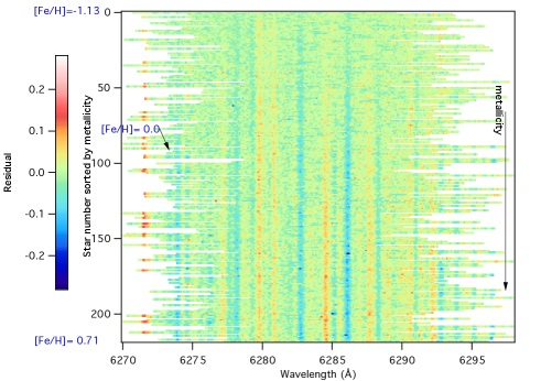
Figure 16: Residuals as a function of wavelength and metallicity for the DIB 6283.8 Å . They form the basis for the EW correction and the error estimate.

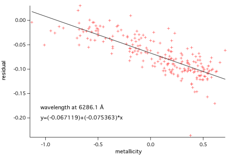
Figure 17: Example of residuals vs -metallicity relationships: here the residuals depend on the metallicity and are negative, which corresponds to an under-predicted stellar absorption line.

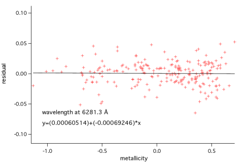
Figure 18: Example of residuals vs -metallicity relationships: here the residuals do not depend on the metallicity and are negligible.

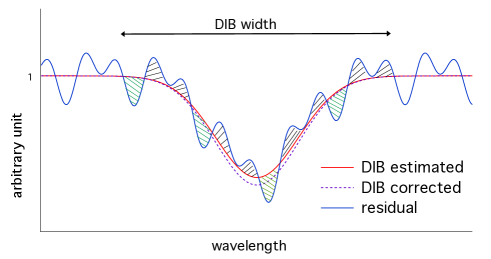
Figure 19: Schematic illustration of the correction applied to the EW measurements. The red curve represents the DIB profile as it comes out from the fitting phase. Hatched surfaces show the offsets applied at each wavelength that are computed for each star, as a function of its metallicity. The dashed line illustrates the corrected DIB.