Multi-discontinuity algorithm for world-line Monte Carlo simulations
Abstract
We introduce a multi-discontinuity algorithm for the efficient global update of world-line configurations in Monte Carlo simulations of interacting quantum systems. This algorithm is a generalization of the two-discontinuity algorithms introduced in Refs. [N. Prokof’ev, B. Svistunov, and I. Tupitsyn, Phys. Lett. A 238, 253 (1998)] and [O. Syljuåsen and A. Sandvik, Phys. Rev. E 66, 046701 (2002)] . This generalization is particularly effective for studying Bose-Einstein condensates (BEC) of composite particles. In particular, we demonstrate the utility of the generalized algorithm by simulating a Hamiltonian for an anti-ferromagnet with strong uniaxial single-ion anisotropy. The multi-discontinuity algorithm not only solves the freezing problem that arises in this limit, but also allows the efficient computing of the off-diagonal correlator that characterizes a BEC of composite particles.
pacs:
02.70.Ss,75.30.KzIntroduction: Cooperative phenomena in quantum systems (e.g., superfluidity, Bose-Einstein condensation, superconductivity, magnetism, etc.) have fascinated physicists for decades. The study of these phenomena often requires one to consider interaction regimes for which traditional perturbative approaches do not work. World-line quantum Monte-Carlo (QMC) simulations based on the Feynman path integral formulation have demonstrated to be a very powerful method for studying systems in these regimes Ceperley (1995); Kawashima and Harada (2004). The main reasons are that the QMC method is unbiased, and its results are exact within statistical error. Therefore, it is imperative to expand the range of applicability of this method by developing QMC algorithms for problems that can not be simulated with state-of-the-art numerical techniques.
Although the worm algorithm Prokof’ev et al. (1998) and the directed-loop algorithm (DLA) Syljuåsen and Sandvik (2002), are the most efficient strategies for global updates in the QMC simulations, they have difficulties when applied to systems exhibiting Bose-Einstein condensates (BECs) of composite particles. BECs of composite particles appear in different contexts, such as bosonic gases of two species ( and ) of ultra cold atoms Kuklov and Svistunov (2003); Söyler et al. (2009) and homonuclear bosonic gases ( Xu et al. (2003), Herbig et al. (2003), etc.). Another simple example of BECs of composite particles is the ferro-nematic magnetic ordering that appears in quantum magnets with single-ion anisotropy Wierschem et al. (2012). In general, high spin systems () whose total magnetization along a particular axis is conserved (it will be our -axis) can exhibit a local order parameter of the form () in the absence of magnetic and any lower moments, i.e., for . These order parameters correspond to different moments of a distribution of electric currents. For instance, corresponds to quadrupolar or nematic order, and corresponds to octupolar order. After mapping the spin system into a gas of bosons, the phase with order parameter is mapped into a BEC of composite particles containing -bosons. For instance, nematic ordering is mapped into a BEC of pairs of bosons Wierschem et al. (2012).
QMC simulations sample and update the dimensional world-line configurations of the quantum system under consideration ( is the spatial dimension). Standard algorithms insert a pair of discontinuities head and tail in the world-line configuration. The head propagates until it meets the tail Kawashima and Harada (2004). The head changes the local states of the world-line configuration along its way. As a result, states on the loop drawn by the head’s trajectory are globally updated. For bosonic systems, the discontinuities typically correspond to the creation, , or annihilation, , of a particle. For QMC simulations of mixtures of bosonic gases Kuklov and Svistunov (2003); Kuklov et al. (2004); Söyler et al. (2009); Guglielmino et al. (2010); Ohgoe and Kawashima (2011); Capogrosso-Sansone (2011); Capogrosso-Sansone and Kuklov (2011); Pollet (2012), including -type and -type bosons, the discontinuities can be of the form or that exchange the type of boson Ohgoe and Kawashima (2011). However, we will see that two discontinuities are not enough to perform efficient simulations in certain cases because of the so-called “freezing problem”. To solve this problem, algorithms with two or more pairs of discontinuities corresponding to , , or have been considered as a generalization of the worm algorithm (e.g. Refs. Söyler et al. (2009); Capogrosso-Sansone and Kuklov (2011); Pollet (2012)). Furthermore the two-discontinuity algorithms often suffer from a serious slowing down problem for calculations of off-diagonal correlators like , which characterize the condensation of composite particles.
In this paper, we present a method called the multi-discontinuity algorithm (MDA) that incorporates an arbitrary number of discontinuities in order to solve the freezing problem. We will show that the MDA can be used for simulating BECs of composite particles that cannot be simulated efficiently with two-discontinuity algorithms. Although the MDA can be applied to many different situations, we will consider a simple example of an antiferromagnetic ( Heisenberg model with external magnetic field, , and single-ion uniaxial anisotropy . We will see that the MDA successfully explores the ferronematic phase of this model, while the DLA fails because of the freezing problem. Since one additional discontinuity is enough for simulating the system, we restrict to three discontinuities in this paper. The extension to the algorithm to more than three discontinuities is straightforward.
Model: We consider the spin-one Hamiltonian
| (1) |
where the summation of runs over all the nearest-neighbor bonds and the model is defined on -dimensional hypercubic lattices Hamer et al. (2010); Wierschem et al. (2012). We restrict the model to the case of easy-axis single-ion anisotropy . In the absence of a magnetic field (), the ground state of exhibits Ising-like antiferromagnetic ordering along the axis (AFM-z). This AFM-z phase is destroyed by the application of a strong enough magnetic field via a first-order quantum phase transition to a new phase that exhibits ferronematic (FN) ordering Wierschem et al. (2012). A further increase of the magnetic field leads to a second order phase transition to the fully polarized phase. As we will see later, the MDA is necessary for finding and studying the FN phase that is characterized by the FN susceptibility,
Algorithm: World-line configurations in the dimensional space introduced in the Feynman path integral formulation are sampled by the QMC method Kawashima and Harada (2004). Here we explain the MDA as a generalization of the DLA by using model (1) as an example of its application. When the DLA is simply applied to model (1) for , it suffers from the negative sign problem. To avoid the negative sign problem, we introduce a spin rotation by along the axis () for the sublattice. The expression of the Hamiltonian in the new basis is
| (2) | |||||
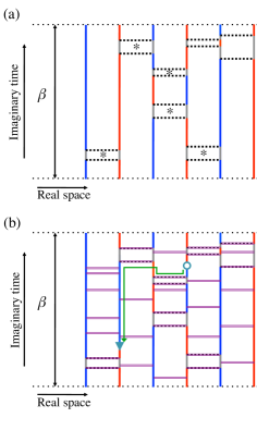
We will start by applying the DLA to see how the freezing problem arises for and . Figure 1(a) shows a typical world-line configuration appearing at and low temperature. Because of the strong anisotropy, , the states are the vast majority, while the states rarely appear in the world-line configurations. The density of these minority states is (note that the volume of the dimensional space has units of inverse energy so the density of states has units of energy). Moreover, the states typically appear forming bubbles that correspond to quantum fluctuations. These quantum fluctuations are crucial for the stabilization of the FN ordering Wierschem et al. (2012). We will see that the bubbles of states are the main source of difficulty for the DLA.
In the DLA algorithm, the world-line configurations are globally updated by introducing a pair of discontinuities called worm and their scattering objects called vertices. The world-line configurations are updated according to the following protocol:
- Step 1
-
Place vertices stochastically (purple double line in Fig. 1(b)). The density of vertices at is a function of .
- Step 2
- Step 3
-
Move the head until it hits a vertex or the tail. If it hits the tail, go to Step 3-1, otherwise, Step 3-2.
- Step 3-1
-
Let the worm annihilate, and go back to Step 2, or go to Step 4.
- Step 3-2
-
Choose its new direction stochastically, and go to Step 3.
- Step 4
-
Erase all vertices after creating and annihilating the worm several times.
More details of the DLA can be found in Ref. Syljuåsen and Sandvik (2002); Kawashima and Harada (2004). The worm is generated by a “source term”, , that is added to the Hamiltonian (). For the case of our model (2), we choose as
| (3) |
The discontinuity is created by any of the four terms , , , or . We sample world-line configurations whose Boltzmann weights are and . In other words, the allowed world-line configurations have only one warm or no discontinuity at all. Because of the external field , the head created by is trapped locally in a bubble, as shown in Fig. 2. The probability of escaping from such a trap is exponentially small in the number of vertices corresponding the term on the way to escape, and it becomes negligibly small because the typical number of the vertices is . As a result, it takes an exponentially long time to complete a cycle of creation and annihilation of a worm. This trapping problem makes the DLA inefficient for simulating the FN phase of .

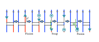
The basic difficulty of the the DLA can be eliminated by considering an enlarged Hilbert space via the inclusion of a third discontinuity. We add a new source term, to , to generate a third discontinuity that has a weight , which can be different from , and sample the world-line configurations whose weights are , , or . Accordingly, we consider three new processes that will be called “fusion”, “fission” and “swap” (see Fig. 3 ). These new processes are executed when the head stops at a newly introduced one-body vertex. Although this new vertex is supposed to be created with a uniform distribution, in practice we create a virtual new vertex Kato et al. (2007); Kato and Kawashima (2009) to avoid the unnecessary proliferation of vertices and the introduction of new free parameters. Fission corresponds to the process by which one discontinuity decays into two discontinuities. We represent these processes by indicating the source operators that create the initial and the final states: [ and ], [ and ], [ and ], and [ and ]. The inverse processes correspond to fusions because they combine two discontinuities into a single one. The swap corresponds to the process of exchanging the head and one of the two tails. To include these three new processes, we need to replace Steps 3, 3-1, and 3-2 of the conventional DLA by the following steps:
- Step 3
-
Calculate . is a random number with uniform distribution in the interval . (See the Appendix for details of virtual placement of vertices.) If , where is the time interval between the head and the next object the head finds on its way (a vertex or another discontinuity), go to Step 3-1, otherwise go to Step 3-2.
- Step 3-1
-
Let the head go to the next object. If the next object is a vertex, go to Step 3-1-1, otherwise go to Step 3-1-2.
- Step 3-1-1
-
Choose a new direction of the head stochastically, and go back to Step 3.
- Step 3-1-2
-
If the total number of discontinuities is , go to Step 3-1-2-1, otherwise go to Step 3-1-2-2.
- Step 3-1-2-1
-
Let the discontinuities annihilate each other, and go back to Step 2, or go to Step 4.
- Step 3-1-2-2
-
Let the two discontinuities fuse and go to Step 3.
- Step 3-2
-
Move the discontinuity through the time interval . If , go to Step 3-2-1, otherwise () go to Step 3-2-2.
- Step 3-2-1
-
Let the head fission, and go to Step 3.
- Step 3-2-2
-
Let the head freeze, exchange discontinuities as a new head to move randomly (swap), and go to Step 3.
The value of the free parameter is fixed so that the average path lengths of the head with and without the third discontinuity are roughly the same.
Example of application: Figure 4 shows the FN susceptibility of model (2) defined on a ring () of spins and for Hamiltonian parameters , and . The three curves are the results obtained by using MDA, DLA and exact diagonalization (ED). The agreement between MDA and ED results is excellent. However, there is a rather large deviation between the DLA and ED results, although the agreement is very good for other physical quantities (e.g., energy and uniform magnetization) that are not shown. This deviation confirms that DLA does not obtain an accurate estimate of the off-diagonal pair-pair correlation function , that determines the FN susceptibility because of a serious slowing down problem. This correlation function is obtained by counting the number of events in which only two discontinuities corresponding to and exist in whole space, with the discontinuity located at and the discontinuity located at Ohgoe and Kawashima (2011). As it is clear from Eq. (Multi-discontinuity algorithm for world-line Monte Carlo simulations), is the integration of the sum of this correlation function over all the possible values of the coordinates and . We sample the whole length of the trajectory of the and discontinuities traveling when no other discontinuity exists. As we explained in the previous section, the DLA suffers from a serious slowing down problem because the head of a worm made of a pair of and discontinuities cannot go through a bubble of states. This limitation precludes the correct estimation of , which is the crucial physical quantity for identifying the FN phase in a finite size system.
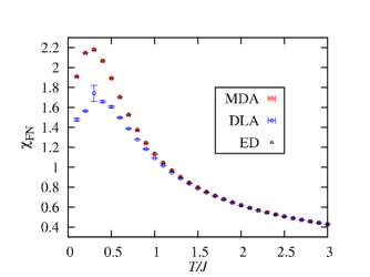
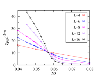
Figure 5 shows the temperature dependence of the conveniently scaled FN susceptibility, , for the case of a simple cubic lattice and Hamiltonian parameters and . The common crossing point among the curves obtained with different system sizes indicates that there is a finite temperature transition between the low temperature FN phase and a high temperature paramagnetic phase. The order parameter of the FN phase is , which in bosonic language can be interpreted as a Bose-Einstein condensate of pairs of bosons. Thus, if continuous, the phase transition should belong to the 3D XY universality class. This is indeed the case according to the scaling analysis shown in Fig. 5: there is a common crossing point when we choose the value of that corresponds to the 3D XY universality class.
Conclusions: In summary, we have introduced a MDA that overcomes some limitations of the two-discontinuity algorithms. The MDA helps to solve the freezing problem that often arises in the simulation of strongly interacting quantum systems. The example that we discussed is just one out of many. Moreover the two-discontinuity algorithms do not satisfy ergodicity for a large class of physically relevant models. In other words, there are physically possible world-line configurations that have not been sampled. For instance, the MDA is also necessary for simulating any quantum spin system with cubic single-ion anisotropy Kawashima and Harada (2004). This is a quite common case for several Mott insulating materials such as EuTiO3 Petrovic et al. .
The extension of the three-discontinuity algorithm to -discontinuity is straightforward, and it is necessary for describing certain physical situations such as antiferromagnets with cubic single-ion anisotropy. The only qualitative difference for is the possibility of creating or annihilating a new pair of discontinuities in world-line configurations that already contain a finite number of discontinuities. For efficient simulations with , we choose the swap or the fission stochastically when the head stops at a virtual vertex with . (We choose the fission with probability 1 when and .) Although we introduced the MDA as a generalization of the DLA in this paper, it is straightforward to modify the MDA in such a way that it becomes a generalization of the worm algorithm.
The successful application of the MDA to the Heisenberg antiferromagnet with uniaxial single-ion anisotropy and Zeeman coupling to an external magnetic field demonstrates the relevance of this method. We showed that the pair-condensation or ferronematic susceptibility, , obtained from simulations based on the MDA accurately reproduces the ED results. The same is not true for the DLA. Our MDA simulations also reproduce the expected finite temperature second order phase transition between the paramagnetic and FN phases in a simple cubic lattice.
Acknowledgements.
I thank K. Wierschem, P. Sengupta, C. D. Batista, and N. Kawashima for fruitful discussions. I also thank A. Kuklov and T. Ohgoe for useful comments on a draft. This research was performed under the U.S. DOE Contract No. DE-AC52-06NA25396 through the LDRD program, and used resources of the NERSC, which is supported by the Office of Science of the U.S. DOE Contract No. DE-AC02-05CH11231.*
Appendix A Fission and fusion
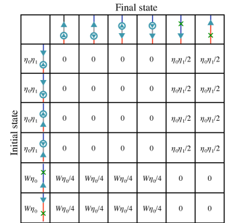
In this appendix, we consider the details of virtual placement of vertices for fission and fusion. We introduce a single-site vertex for the fission and fusion processes. The weight of the vertex is uniform everywhere and independent from the local state of the world-line. We set so that the acceptance probability of fusion is equal to unity. We start by considering the time-reversal symmetry of the algorithm that is a sufficient condition for satisfying detailed balance Kawashima and Harada (2004). Here, we will only consider the time-reversal symmetry condition associated with the fission and fusion processes. We decompose the weights just before a fission or fusion operation as where is the weight of the initial configuration . By using the partial weights, , we determine the transition probability from to as , so that the time-reversal symmetry condition, , is satisfied. Typically, we take for simplicity. Figure 6 shows an example of of the fission and fusion processes. The table is symmetric when and the time-reversal symmetry condition is satisfied. “Virtual placement of a vertex” means finding the next point along the world line where the head is scattered. The vertices are generated based on a Poisson distribution with density . Namely, the time interval to the next vertex is , where is random number between 0 and 1: .
References
- Ceperley (1995) D. M. Ceperley, Rev. Mod. Phys. 67, 279 (1995).
- Kawashima and Harada (2004) N. Kawashima and K. Harada, J. Phys. Soc. Jpn. 73, 1379 (2004).
- Prokof’ev et al. (1998) N. Prokof’ev, B. Svistunov, and I. Tupitsyn, Phys. Lett. A 238, 253 (1998).
- Syljuåsen and Sandvik (2002) O. F. Syljuåsen and A. W. Sandvik, Phys. Rev. E 66, 046701 (2002).
- Kuklov and Svistunov (2003) A. B. Kuklov and B. V. Svistunov, Phys. Rev. Lett. 90, 100401 (2003).
- Söyler et al. (2009) Ş. Söyler, B. Capogrosso-Sansone, N. Prokof’ev, and B. Svistunov, New J. Phys. 11, 073036 (2009).
- Xu et al. (2003) K. Xu, T. Mukaiyama, J. R. Abo-Shaeer, J. K. Chin, D. E. Miller, and W. Ketterle, Phys. Rev. Lett. 91, 210402 (2003).
- Herbig et al. (2003) J. Herbig, T. Kraemer, M. Mark, T. Weber, C. Chin, H. Nägerl, and R. Grimm, Science 301, 1510 (2003).
- Wierschem et al. (2012) K. Wierschem, Y. Kato, Y. Nishida, C. Batista, and P. Sengupta, Phys. Rev. B 86, 201108(R) (2012).
- Kuklov et al. (2004) A. Kuklov, N. Prokof’ev, and B. Svistunov, Phys. Rev. Lett. 92, 050402 (2004).
- Guglielmino et al. (2010) M. Guglielmino, V. Penna, and B. Capogrosso-Sansone, Phys. Rev. A 82, 021601 (2010).
- Ohgoe and Kawashima (2011) T. Ohgoe and N. Kawashima, Phys. Rev. A 83, 023622 (2011).
- Capogrosso-Sansone (2011) B. Capogrosso-Sansone, Phys. Rev. A 83, 053611 (2011).
- Capogrosso-Sansone and Kuklov (2011) B. Capogrosso-Sansone and A. Kuklov, Journal of Low Temperature Physics 165, 213 (2011).
- Pollet (2012) L. Pollet, Rep. Prog. Phys. 75, 094501 (2012).
- Hamer et al. (2010) C. J. Hamer, O. Rojas, and J. Oitmaa, Phys. Rev. B 81, 214424 (2010).
- Kato et al. (2007) Y. Kato, T. Suzuki, and N. Kawashima, Phys. Rev. E 75, 066703 (2007).
- Kato and Kawashima (2009) Y. Kato and N. Kawashima, Phys. Rev. E 79, 021104 (2009).
- Hasenbusch and Török (1999) M. Hasenbusch and T. Török, J. Phys. A: Math. Gen. 32, 6361 (1999).
- (20) A. P. Petrovic, Y. Kato, S. Sunku, T. Ito, P. Sengupta, L. Spalek, M. Shimuta, T. Katsufuji, C. Batista, S. Saxena, et al., arXiv:1204.0150.