Cosmic propagators at two-loop order

Francis Bernardeau Institut de Physique Th orique, CEA, IPhT, F-91191 Gif-sur-Yvette, France CNRS, URA 2306, F-91191 Gif-sur-Yvette, France    Atsushi Taruya Research Center for the Early Universe, School of Science, The University of Tokyo, Bunkyo-ku, Tokyo 113-0033, Japan Kavli Institute for the Physics and Mathematics of the Universe, Todai Institutes for Advanced Study, the University of Tokyo, Kashiwa, Chiba 277-8583, Japan (Kavli IPMU, WPI)    Takahiro Nishimichi Kavli Institute for the Physics and Mathematics of the Universe, Todai Institutes for Advanced Study, the University of Tokyo, Kashiwa, Chiba 277-8583, Japan (Kavli IPMU, WPI)
Abstract

We explore the properties of two-point cosmic propagators when Perturbation Theory (PT) loop corrections are consistently taken into account. We show in particular how the interpolation scheme proposed in Bernardeau et al. (2011) can be explicitly used up to two-loop order introducing the notion of regular parts for the contributing terms. Extending the one-loop results, we then derive and give semi analytical forms of the two-loop contributions for both the cosmic density and velocity propagators. These results are tested against numerical simulations and shown to significantly improve upon one-loop results for redshifts above 0.50.50.5.
We found however that at lower redshift two-loop order corrections are too large partly due to a strong sensitivity of those terms to the small scale modes. We show that this dependence is expected to be even larger for higher order loop corrections both from theoretical investigations and numerical tests, the latter obtained with Monte Carlo evaluations of the three-loop contributions. This makes small-scale regularization schemes necessary for the use of such higher order corrections.

pacs:
98.80.-k, 98.65.-r

I Introduction

Precision measurements of the statistical properties of the large-scale structure of the universe is the key to current large projects of observational cosmology. They aim in particular at measuring the galaxy power spectrum at the scales where Baryonic Acoustic Oscillations can be detected (Eisenstein et al. (2005); Percival et al. (2007); Blake et al. (2011); Nuza et al. (2012)) or at measuring the projected density power spectrum from weak lensing observations (as stressed in Albrecht et al. (2006) and which is the part of the core program of the Euclid mission Laureijs et al. (2011)). In this context, semi-analytic tools are now developed that aim at computing, from first principles, the statistical properties of the cosmic fields at large-scale. Standard Perturbation Theory approaches (see Bernardeau et al. (2002)) are however not very efficient in producing well behaved next-to-leading order terms to the spectra or bispectra. It leads indeed to a resummation series that has poor converging properties (see Crocce and Scoccimarro (2006a) for more insights into that). Alternative approaches have been recently developed that propose, implicitly or explicitly, a reorganization of the perturbation series. This is the case in particular for the Renormalization Perturbation Theory (RPT) approaches developed initially in Crocce and Scoccimarro (2006a). Other approaches are based on the writing of closed system of integro-differential equations as in the closure theory approach, Taruya and Hiramatsu (2008), or in the Time Flow equation hierarchy presented in Pietroni (2008). We put ourselves in the context of the RPT approaches and its extensions which are based on the introduction of the two-point propagator and on a re-writing of the series expansion with the help of that object. A related but alternative approach has been proposed in Bernardeau et al. (2008) where was introduced the concepts of multi-point propagators. Interaction vertices can then be formally renormalized as well. It has been shown there that a new scheme for the computation of spectra and poly-spectra can be obtained form the multi-point propagators, from the the so-called ΓΓ\Gamma expansion.

The focus of this paper is precisely on the behavior of the two-point propagator and on the precision one can theoretically attain in its description. In particular one wishes to evaluate the importance of the multi-loop corrections to its expression, in practice up to second order, and to see whether these corrections can be safely computed. Comparisons with N-body codes will be used taking advantage of the interpolation scheme proposed in Bernardeau et al. (2011). In this paper it is indeed shown how multi-loop corrections can be consistently used to get predictions on multi-propagator expressions with theoretically increasing precision. These investigations aim in particular at pinning down the validity range of this type of calculations. As we will see in the following the two-point propagator is the quantity, at a given order in PT, that is the most sensitive to high-k𝑘k modes in the computation of power spectra. Quantifying the importance of the small scale physics, for large-scale predictions, is a daunting quest. Some phenomenological results have been proposed in Pueblas and Scoccimarro (2009); Valageas (2010) to investigate for instance the importance of shell crossings. This is also the idea behind the works in Pietroni et al. (2011); Carrasco et al. (2012) where the impact of the small scale physics is tentatively introduced as extra source terms. In this paper we eventually investigate this problem from a PT approach.

The paper is organized as follows. In Sec. II we recall the motion equations for gravitational instabilities of a cosmic fluid. In Sec. III we compute the two-loop corrective terms and propose analytic fits for them. In Sect. IV we first estimate the contributions of the three-loop terms from Monte-Carlo computations. Our results are tested with the help of consistency relation we provided in Sect. III. We then explore in more detail the expected properties of the loop corrections at arbitrary orders introducing the notion of kernels and henceforth quantifying the sensitivity of the results to large and small scales modes. Our concluding remarks are presented in Sec. V.

II The cosmic two-point propagators

II.1 The equations of motion

We are interested here in the development of cosmological instabilities in a cosmological dust fluid. In general the dynamical evolution of such a fluid can be described with the Vlasov equation. As usual we then restrict our investigations to the regime where multi-flow regions play a negligible role but we will discuss this assumption later on. In the one flow limit, the motion equation then takes the form of a set of three coupled equations relating the local density contrast, the peculiar velocity field and the gravitational potential (see Bernardeau et al. (2002)).

At linear order these equations can easily be solved for an arbitrary background cosmology. One generically finds a growing solution and a decaying solution. Let us denotes D+(τ)subscript𝐷𝜏D_{+}(\tau) the growing mode solution for the density contrast f+(τ)subscript𝑓𝜏f_{+}(\tau) its logarithmic derivative with respect to the expansion so that,

δ(𝐤,η)=D+(η)δ0(𝐤),θ(𝐤,η)/=f+(η)D+(η)δ0(𝐤)formulae-sequence𝛿𝐤𝜂subscript𝐷𝜂subscript𝛿0𝐤𝜃𝐤𝜂subscript𝑓𝜂subscript𝐷𝜂subscript𝛿0𝐤\delta({\bf k},\eta)=D_{+}(\eta)\delta_{0}({\bf k}),\ \ \theta({\bf k},\eta)/{\cal H}=-f_{+}(\eta)D_{+}(\eta)\delta_{0}({\bf k}) (1)

is the solution for the growing mode and similarly,

δ(𝐤,η)=D(η)δ0(𝐤),θ(𝐤,η)/=f(η)D(η)δ0(𝐤)formulae-sequence𝛿𝐤𝜂subscript𝐷𝜂subscript𝛿0𝐤𝜃𝐤𝜂subscript𝑓𝜂subscript𝐷𝜂subscript𝛿0𝐤\delta({\bf k},\eta)=D_{-}(\eta)\delta_{0}({\bf k}),\ \ \theta({\bf k},\eta)/{\cal H}=-f_{-}(\eta)D_{-}(\eta)\delta_{0}({\bf k}) (2)

for the decaying.

Following Scoccimarro (1998), the motion equations describing a pressure-less fluid in the one-flow limit can be written in a compact form with the use of the doublet Ψa(𝐤,τ)subscriptΨ𝑎𝐤𝜏\Psi_{a}({\bf k},\tau), defined as,

Ψa(𝐤,τ)(δ(𝐤,τ),1f+(τ)θ(𝐤,τ)),subscriptΨ𝑎𝐤𝜏𝛿𝐤𝜏1subscript𝑓𝜏𝜃𝐤𝜏\Psi_{a}({\bf k},\tau)\equiv\Big{(}\delta({\bf k},\tau),\ -\frac{1}{f_{+}(\tau)\cal H}\theta({\bf k},\tau)\Big{)}, (3)

where dlna/dτ𝑑𝑎𝑑𝜏{\cal H}\equiv{d\ln a/{d\tau}} is the conformal expansion rate with a(τ)𝑎𝜏a(\tau) the cosmological scale factor and τ𝜏\tau the conformal time and where the index a=1,2𝑎12a=1,2 selects the density or velocity components and which makes explicit use of the growing solution.

It is then convenient to re-express the time dependence in terms of the growing solution and in the following we will use the time variable η𝜂\eta defined as

η=logD+(η)𝜂subscript𝐷𝜂\eta=\log{D_{+}(\eta)} (4)

assuming the growing factor is set to unity at initial time. Then the fully nonlinear equations of motion in Fourier space read Bernardeau et al. (2002) (we henceforth use the convention that repeated Fourier arguments are integrated over and the Einstein convention on repeated indices),

ηΨa(𝐤,η)+Ωab(η)Ψb(𝐤,η)𝜂subscriptΨ𝑎𝐤𝜂subscriptΩ𝑎𝑏𝜂subscriptΨ𝑏𝐤𝜂\displaystyle\frac{\partial}{\partial\eta}\Psi_{a}({\bf k},\eta)+\Omega_{ab}(\eta)\Psi_{b}({\bf k},\eta) =\displaystyle= γabc(𝐤,𝐤1,𝐤2)Ψb(𝐤1,η)Ψc(𝐤2,η),subscript𝛾𝑎𝑏𝑐𝐤subscript𝐤1subscript𝐤2subscriptΨ𝑏subscript𝐤1𝜂subscriptΨ𝑐subscript𝐤2𝜂\displaystyle\gamma_{abc}({\bf k},{\bf k}_{1},{\bf k}_{2})\ \Psi_{b}({\bf k}_{1},\eta)\ \Psi_{c}({\bf k}_{2},\eta), (5)

where

Ωab(η)[0132Ωmf+232Ωmf+21],subscriptΩ𝑎𝑏𝜂delimited-[]0132subscriptΩ𝑚superscriptsubscript𝑓232subscriptΩ𝑚superscriptsubscript𝑓21\Omega_{ab}(\eta)\equiv\Bigg{[}\begin{array}[]{cc}0&-1\\ -\frac{3}{2}\frac{\Omega_{m}}{f_{+}^{2}}&\frac{3}{2}\frac{\Omega_{m}}{f_{+}^{2}}-1\end{array}\Bigg{]}, (6)

and the symmetrized vertex matrix γabcsubscript𝛾𝑎𝑏𝑐\gamma_{abc} describes the non linear interactions between different Fourier modes. Its components are given by

γ222(𝐤,𝐤1,𝐤2)subscript𝛾222𝐤subscript𝐤1subscript𝐤2\displaystyle\gamma_{222}({\bf k},{\bf k}_{1},{\bf k}_{2}) =\displaystyle= δD(𝐤𝐤1𝐤2)|𝐤1+𝐤2|2(𝐤1𝐤2)2k12k22,subscript𝛿D𝐤subscript𝐤1subscript𝐤2superscriptsubscript𝐤1subscript𝐤22subscript𝐤1subscript𝐤22superscriptsubscript𝑘12superscriptsubscript𝑘22\displaystyle\delta_{\rm D}({\bf k}-{\bf k}_{1}-{\bf k}_{2})\ {|{\bf k}_{1}+{\bf k}_{2}|^{2}({\bf k}_{1}\cdot{\bf k}_{2})\over{2k_{1}^{2}k_{2}^{2}}},
γ121(𝐤,𝐤1,𝐤2)subscript𝛾121𝐤subscript𝐤1subscript𝐤2\displaystyle\gamma_{121}({\bf k},{\bf k}_{1},{\bf k}_{2}) =\displaystyle= δD(𝐤𝐤1𝐤2)(𝐤1+𝐤2)𝐤12k12,subscript𝛿D𝐤subscript𝐤1subscript𝐤2subscript𝐤1subscript𝐤2subscript𝐤12superscriptsubscript𝑘12\displaystyle\delta_{\rm D}({\bf k}-{\bf k}_{1}-{\bf k}_{2})\ {({\bf k}_{1}+{\bf k}_{2})\cdot{\bf k}_{1}\over{2k_{1}^{2}}}, (7)

γabc(𝐤,𝐤a,𝐤b)=γacb(𝐤,𝐤b,𝐤a)subscript𝛾𝑎𝑏𝑐𝐤subscript𝐤𝑎subscript𝐤𝑏subscript𝛾𝑎𝑐𝑏𝐤subscript𝐤𝑏subscript𝐤𝑎\gamma_{abc}({\bf k},{\bf k}_{a},{\bf k}_{b})=\gamma_{acb}({\bf k},{\bf k}_{b},{\bf k}_{a}), and γ=0𝛾0\gamma=0 otherwise, where δDsubscript𝛿D\delta_{\rm D} denotes the Dirac delta distribution. The matrix γabcsubscript𝛾𝑎𝑏𝑐\gamma_{abc} is independent on time (and on the background evolution) and encodes all the non-linear couplings of the system. The formal integral solution to Eq. (5) is given by (see Scoccimarro (1998, 2001); Crocce and Scoccimarro (2006a) for a detailed derivation)

Ψa(𝐤,η)subscriptΨ𝑎𝐤𝜂\displaystyle\Psi_{a}({\bf k},\eta) =\displaystyle= gab(η)ϕb(𝐤)+0ηdηgab(η,η)γbcd(s)(𝐤,𝐤1,𝐤2)Ψc(𝐤1,η)Ψd(𝐤2,η),subscript𝑔𝑎𝑏𝜂subscriptitalic-ϕ𝑏𝐤superscriptsubscript0𝜂differential-dsuperscript𝜂subscript𝑔𝑎𝑏𝜂superscript𝜂superscriptsubscript𝛾𝑏𝑐𝑑s𝐤subscript𝐤1subscript𝐤2subscriptΨ𝑐subscript𝐤1superscript𝜂subscriptΨ𝑑subscript𝐤2superscript𝜂\displaystyle g_{ab}(\eta)\ \phi_{b}({\bf k})+\int_{0}^{\eta}{{\rm d}\eta^{\prime}}\ g_{ab}(\eta,\eta^{\prime})\ \gamma_{bcd}^{(\rm s)}({\bf k},{\bf k}_{1},{\bf k}_{2})\Psi_{c}({\bf k}_{1},\eta^{\prime})\Psi_{d}({\bf k}_{2},\eta^{\prime}), (8)

where ϕa(𝐤)Ψa(𝐤,η=0)subscriptitalic-ϕ𝑎𝐤subscriptΨ𝑎𝐤𝜂0\phi_{a}({\bf k})\equiv\Psi_{a}({\bf k},\eta=0) denotes the initial conditions, set when the growth factor D+=1subscript𝐷1D_{+}=1 and where gab(η)subscript𝑔𝑎𝑏𝜂g_{ab}(\eta) is the linear propagator that is Green’s function of the linearized version of Eq. (5) and describes the standard linear evolution of the density and velocity fields from their initial state.

In the following calculations we will be using the value of the ΩabsubscriptΩ𝑎𝑏\Omega_{ab} matrix to be that of the Einstein de Sitter background that is effectively assuming that Dsubscript𝐷D_{-} scales like D+3/2superscriptsubscript𝐷32D_{+}^{-3/2}. This is known to be a very good approximation even in the context of a Λlimit-fromΛ\Lambda-CDM universe (see for instance Crocce et al. (2012) for an explicit investigation of the consequences of such an approximation).

The ensemble average of any quantity can then be built out of those of the initial fields. They are entirely defined from the initial power spectrum of density fluctuations Pab(k)subscript𝑃𝑎𝑏𝑘P_{ab}(k) define as,

<ϕa(𝐤)ϕb(𝐤)>=δD(𝐤+𝐤)Pab(k).expectationsubscriptitalic-ϕ𝑎𝐤subscriptitalic-ϕ𝑏superscript𝐤subscript𝛿D𝐤superscript𝐤subscript𝑃𝑎𝑏𝑘\big{<}\phi_{a}({\bf k})\phi_{b}({\bf k}^{\prime})\big{>}=\delta_{\rm D}({\bf k}+{\bf k}^{\prime})P_{ab}(k). (9)

In what follows most of the calculations and applications will be made assuming initial conditions in the growing mode, for which ϕa(𝐤)=δ0(𝐤)uasubscriptitalic-ϕ𝑎𝐤subscript𝛿0𝐤subscript𝑢𝑎\phi_{a}({\bf k})=\delta_{0}({\bf k})u_{a} with ua=(1,1)subscript𝑢𝑎11u_{a}=(1,1), and therefore with Pab(k)=P0(k)uaubsubscript𝑃𝑎𝑏𝑘subscript𝑃0𝑘subscript𝑢𝑎subscript𝑢𝑏P_{ab}(k)=P_{0}(k)u_{a}u_{b}.

II.2 Definition and general properties of the two-point and multi-point propagators

The gab(s)subscript𝑔𝑎𝑏𝑠g_{ab}(s) appears clearly to be one of the key ingredient of these constructions. It can be described as the the linear propagator giving the variation of the mode amplitude as time is running. The idea at the heart of the RPT approach is to generalize this operator beyond linear theory. More specifically the quantity Ψa(𝐤,s)ϕb(𝐤)subscriptΨ𝑎𝐤𝑠subscriptitalic-ϕ𝑏superscript𝐤\frac{\partial\Psi_{a}({\bf k},s)}{\partial\phi_{b}({\bf k}^{\prime})} expresses the way Ψa(𝐤,s)subscriptΨ𝑎𝐤𝑠\Psi_{a}({\bf k},s) depends on ϕb(𝐤)subscriptitalic-ϕ𝑏superscript𝐤\phi_{b}({\bf k}^{\prime}) as a function of time s𝑠s. This function however depends on the stochastic properties of the fields. One can nonetheless define its ensemble average, Gab(𝐤)subscript𝐺𝑎𝑏𝐤G_{ab}({\bf k}), as

Ψa(𝐤,η)ϕb(𝐤)=δD(𝐤𝐤)Gab(k;η).delimited-⟨⟩subscriptΨ𝑎𝐤𝜂subscriptitalic-ϕ𝑏superscript𝐤subscript𝛿D𝐤superscript𝐤subscript𝐺𝑎𝑏𝑘𝜂\left<\frac{\partial\Psi_{a}({\bf k},\eta)}{\partial\phi_{b}({\bf k}^{\prime})}\right>=\delta_{\rm D}{\left({\bf k}-{\bf k}^{\prime}\right)}\,G_{ab}(k;\eta). (10)

This quantity depends on the initial fluctuations through the mode couplings. The ensemble average is made precisely over these modes. The Dirac-δ𝛿\delta function it leads to is due, as usual, to the homogeneity of the underlying statistical process. More generally one can define the (p+1)𝑝1(p+1)-point propagators Γ(p)superscriptΓ𝑝\Gamma^{(p)} as (see Bernardeau et al. (2008)),

1p!δpΨa(𝐤,η)δϕb1(𝐤1)δϕbp(𝐤p)=δD(𝐤𝐤1𝐤p)Γab1bp(p)(𝐤1,,𝐤p;η).1𝑝delimited-⟨⟩superscript𝛿𝑝subscriptΨ𝑎𝐤𝜂𝛿subscriptitalic-ϕsubscript𝑏1subscript𝐤1𝛿subscriptitalic-ϕsubscript𝑏𝑝subscript𝐤𝑝subscript𝛿D𝐤subscript𝐤1subscript𝐤𝑝subscriptsuperscriptΓ𝑝𝑎subscript𝑏1subscript𝑏𝑝subscript𝐤1subscript𝐤𝑝𝜂\frac{1}{p!}\left<\frac{\delta^{p}\Psi_{a}({\bf k},\eta)}{\delta\phi_{b_{1}}({\bf k}_{1})\dots\delta\phi_{b_{p}}({\bf k}_{p})}\right>=\delta_{\rm D}{\left({\bf k}-{\bf k}_{1}-\dots-{\bf k}_{p}\right)}\,\Gamma^{(p)}_{ab_{1}\dots b_{p}}({\bf k}_{1},\dots,{\bf k}_{p};\eta). (11)

The Dirac δ𝛿\delta-function that appears in this expression is a direct consequence of the assumed statistical isotropy of space. Note that the propagators can be defined for any time interval. We will however use it here assuming the early time to be the initial time for which one can assume that the cosmic modes correspond to the Matter Dominated era growing mode (see Audren and Lesgourgues (2011) for explicit investigations of the validity of such an approximation). In computing the power spectrum or bispectrum, it is convenient to introduce the reduced propagators as

Γa(p)(𝐤1,,𝐤p;η)=Γab1bp(p)(𝐤1,,𝐤p;η)ub1ubp.superscriptsubscriptΓ𝑎𝑝subscript𝐤1subscript𝐤𝑝𝜂subscriptsuperscriptΓ𝑝𝑎subscript𝑏1subscript𝑏𝑝subscript𝐤1subscript𝐤𝑝𝜂subscript𝑢subscript𝑏1subscript𝑢subscript𝑏𝑝\Gamma_{a}^{(p)}({\bf k}_{1},\dots,{\bf k}_{p};\eta)=\Gamma^{(p)}_{ab_{1}\dots b_{p}}({\bf k}_{1},\dots,{\bf k}_{p};\eta)u_{b_{1}}\dots u_{b_{p}}. (12)

Our main interest here is the late time evolution of the propagators keeping only the most growing modes contributions. In particular, in the following we compute the expression of Gabsubscript𝐺𝑎𝑏G_{ab} order by order in perturbation theory, up to two loop order. Such results can be obtained from a formal expansion of Ψa(𝐤,η)subscriptΨ𝑎𝐤𝜂\Psi_{a}({\bf k},\eta) with respect to the initial field,

Ψa(𝐤,η)=n=1Ψa(n)(𝐤,η)subscriptΨ𝑎𝐤𝜂superscriptsubscript𝑛1superscriptsubscriptΨ𝑎𝑛𝐤𝜂\Psi_{a}({\bf k},\eta)=\sum_{n=1}^{\infty}\Psi_{a}^{(n)}({\bf k},\eta) (13)

with

Ψa(n)(𝐤,η)=d3𝐤1d3𝐤nδD(𝐤𝐤1n)ab1b2bn(n)(𝐤1,,𝐤n;η)ϕb1(𝐤1)ϕbn(𝐤n)superscriptsubscriptΨ𝑎𝑛𝐤𝜂superscriptd3subscript𝐤1superscriptd3subscript𝐤𝑛subscript𝛿D𝐤subscript𝐤1𝑛subscriptsuperscript𝑛𝑎subscript𝑏1subscript𝑏2subscript𝑏𝑛subscript𝐤1subscript𝐤𝑛𝜂subscriptitalic-ϕsubscript𝑏1subscript𝐤1subscriptitalic-ϕsubscript𝑏𝑛subscript𝐤𝑛\displaystyle\Psi_{a}^{(n)}({\bf k},\eta)=\int{\rm d}^{3}{\bf k}_{1}\dots\rm d^{3}{\bf k}_{n}\ \delta_{\rm D}({\bf k}-{\bf k}_{1\dots n})\,{\cal F}^{(n)}_{ab_{1}b_{2}\ldots b_{n}}({\bf k}_{1},\dots,{\bf k}_{n};\eta)\phi_{b_{1}}({\bf k}_{1})\dots\phi_{b_{n}}({\bf k}_{n}) (14)

where (n)superscript𝑛{\cal F}^{(n)} are fully symmetric functions of the wave-vectors. Note that these functions have in general a non-trivial time dependence because they also include sub-leading terms in η𝜂\eta. Their fastest growing term is of course given by the well known {Fn,Gn}subscript𝐹𝑛subscript𝐺𝑛\{F_{n},G_{n}\} kernels in PT (assuming growing mode initial conditions),

ab1b2bn(n)(𝐤1,,𝐤n;η)ub1ubn=exp(nη)Fa(n)(𝐤1,..,𝐤n){\cal F}^{(n)}_{ab_{1}b_{2}\ldots b_{n}}({\bf k}_{1},\dots,{\bf k}_{n};\eta)u_{b_{1}}\ldots u_{b_{n}}=\exp(n\eta)\ F_{a}^{(n)}({\bf k}_{1},..,{\bf k}_{n})

with F1(n)=Fnsuperscriptsubscript𝐹1𝑛subscript𝐹𝑛F_{1}^{(n)}=F_{n} and F2(n)=Gnsuperscriptsubscript𝐹2𝑛subscript𝐺𝑛F_{2}^{(n)}=G_{n} (density or velocity divergence fields respectively). Those quantities can obviously be computed in a standard Perturbation Theory approach. Formally one can then writes,

Γa(p)=Γa,tree(p)+Γa,1loop(p)+Γa,2loop(p)+Γa,3loop(p)+.superscriptsubscriptΓ𝑎𝑝superscriptsubscriptΓ𝑎tree𝑝superscriptsubscriptΓ𝑎1loop𝑝superscriptsubscriptΓ𝑎2loop𝑝superscriptsubscriptΓ𝑎3loop𝑝\Gamma_{a}^{(p)}=\Gamma_{a,\rm tree}^{(p)}+\Gamma_{a,{\rm 1-loop}}^{(p)}+\Gamma_{a,{\rm 2-loop}}^{(p)}+\Gamma_{a,{\rm 3-loop}}^{(p)}+\dots. (15)

When keeping, for each term, the only fastest growing mode, the expressions for the perturbative corrections, Γa,nloop(p)superscriptsubscriptΓ𝑎nloop𝑝\Gamma_{a,{\rm n-loop}}^{(p)} can be rather simplified and written in terms of the standard PT kernels. Those expressions can be written more specifically for the two-point propagators. Let us define then the 2 propagators G1+subscript𝐺limit-from1G_{1+} and G2+subscript𝐺limit-from2G_{2+} as,

G1+(k,η)subscript𝐺limit-from1𝑘𝜂\displaystyle G_{1+}(k,\eta) =\displaystyle= G1a(k,η)ua=G11(k,η)+G12(k,η)subscript𝐺1𝑎𝑘𝜂subscript𝑢𝑎subscript𝐺11𝑘𝜂subscript𝐺12𝑘𝜂\displaystyle G_{1a}(k,\eta)u_{a}=G_{11}(k,\eta)+G_{12}(k,\eta) (16)
G2+(k,η)subscript𝐺limit-from2𝑘𝜂\displaystyle G_{2+}(k,\eta) =\displaystyle= G2a(k,η)ua=G21(k,η)+G22(k,η),subscript𝐺2𝑎𝑘𝜂subscript𝑢𝑎subscript𝐺21𝑘𝜂subscript𝐺22𝑘𝜂\displaystyle G_{2a}(k,\eta)u_{a}=G_{21}(k,\eta)+G_{22}(k,\eta), (17)

for which we have,

Ga+1loop(k,η)superscriptsubscript𝐺limit-from𝑎1loop𝑘𝜂\displaystyle G_{a+}^{{\rm 1-loop}}(k,\eta) =\displaystyle= 3e3ηd3𝐪Fa(3)(𝐪,𝐪,𝐤)P0(q)3superscript𝑒3𝜂superscriptd3𝐪subscriptsuperscript𝐹3𝑎𝐪𝐪𝐤subscript𝑃0𝑞\displaystyle 3\,e^{3\eta}\,\int{\rm d}^{3}{\bf q}\,F^{(3)}_{a}({\bf q},-{\bf q},{\bf k})P_{0}(q) (18)
Ga+2loop(k,η)superscriptsubscript𝐺limit-from𝑎2loop𝑘𝜂\displaystyle G_{a+}^{{\rm 2-loop}}(k,\eta) =\displaystyle= 15e5ηd3𝐪1d3𝐪2Fa(5)(𝐪1,𝐪1,𝐪2,𝐪2,𝐤)P0(q1)P0(q2)15superscript𝑒5𝜂superscriptd3subscript𝐪1superscriptd3subscript𝐪2subscriptsuperscript𝐹5𝑎subscript𝐪1subscript𝐪1subscript𝐪2subscript𝐪2𝐤subscript𝑃0subscript𝑞1subscript𝑃0subscript𝑞2\displaystyle 15\,e^{5\eta}\,\int{\rm d}^{3}{\bf q}_{1}{\rm d}^{3}{\bf q}_{2}\,F^{(5)}_{a}({\bf q}_{1},-{\bf q}_{1},{\bf q}_{2},-{\bf q}_{2},{\bf k})P_{0}(q_{1})P_{0}(q_{2}) (19)

with qi=|𝐪i|subscript𝑞𝑖subscript𝐪𝑖q_{i}=|{\bf q}_{i}| and where the function Fa(m)superscriptsubscript𝐹𝑎𝑚F_{a}^{(m)} are the symmetrized PT kernels of the m𝑚m-th order. One can generalize the above expressions to the one at a general n𝑛n-loop order111This can be further generalized to the n𝑛n-loop correction to the p𝑝p-point propagator: Γnloop(p)(𝐤1,,𝐤p;η)=sn(p)e(2n+1)ηd3𝐪1d3𝐪nFa(2n+p)(𝐪1,𝐪1,,𝐪n,𝐪n,𝐤1,,𝐤p)P0(q1)P0(qn)superscriptsubscriptΓnloop𝑝subscript𝐤1subscript𝐤𝑝𝜂superscriptsubscript𝑠𝑛𝑝superscript𝑒2𝑛1𝜂superscriptd3subscript𝐪1superscriptd3subscript𝐪𝑛subscriptsuperscript𝐹2𝑛𝑝𝑎subscript𝐪1subscript𝐪1subscript𝐪𝑛subscript𝐪𝑛subscript𝐤1subscript𝐤𝑝subscript𝑃0subscript𝑞1subscript𝑃0subscript𝑞𝑛\Gamma_{{\rm n-loop}}^{(p)}({\bf k}_{1},\dots,{\bf k}_{p};\eta)=s_{n}^{(p)}e^{(2n+1)\eta}\int{\rm d}^{3}{\bf q}_{1}\dots\rm d^{3}{\bf q}_{n}\,F^{(2n+p)}_{a}({\bf q}_{1},-{\bf q}_{1},\dots,{\bf q}_{n},-{\bf q}_{n},{\bf k}_{1},\dots,{\bf k}_{p})P_{0}(q_{1})\dots P_{0}(q_{n}) with sn(p)=(2n+p)!(2n1)!!/p!2superscriptsubscript𝑠𝑛𝑝2𝑛𝑝double-factorial2𝑛1superscript𝑝2s_{n}^{(p)}={(2n+p)!(2n-1)!!}/{p!^{2}},

Ga+nloop=sn(1)e(2n+1)ηd3𝐪1d3𝐪nFa(2n+1)(𝐪1,𝐪1,,𝐪n,𝐪n,𝐤)P0(q1)P0(qn)superscriptsubscript𝐺limit-from𝑎nloopsuperscriptsubscript𝑠𝑛1superscript𝑒2𝑛1𝜂superscriptd3subscript𝐪1superscriptd3subscript𝐪𝑛subscriptsuperscript𝐹2𝑛1𝑎subscript𝐪1subscript𝐪1subscript𝐪𝑛subscript𝐪𝑛𝐤subscript𝑃0subscript𝑞1subscript𝑃0subscript𝑞𝑛G_{a+}^{{\rm n-loop}}=s_{n}^{(1)}\,e^{(2n+1)\eta}\int{\rm d}^{3}{\bf q}_{1}\dots\rm d^{3}{\bf q}_{n}\,F^{(2n+1)}_{a}({\bf q}_{1},-{\bf q}_{1},\dots,{\bf q}_{n},-{\bf q}_{n},{\bf k})P_{0}(q_{1})\dots P_{0}(q_{n}) (20)

with a symmetry factor given by

sn(1)=2n+1n!Πj=1n(2j2)=(2n+1)!!.superscriptsubscript𝑠𝑛12𝑛1𝑛superscriptsubscriptΠ𝑗1𝑛2𝑗2double-factorial2𝑛1s_{n}^{(1)}=\frac{2n+1}{n!}\Pi_{j=1}^{n}\left(\begin{array}[]{c}2j\\ 2\end{array}\right)=(2n+1)!!. (21)

Note that the explicit expressions for the standard PT kernels can be obtained from the recursion relations (see also Bernardeau et al. (2002)),

Fa(1)(𝐤1)superscriptsubscript𝐹𝑎1subscript𝐤1\displaystyle F_{a}^{(1)}({\bf k}_{1}) =\displaystyle= {1,1},11\displaystyle\{1,1\}, (22)
Fa(n)(𝐤1,,𝐤n)superscriptsubscript𝐹𝑎𝑛subscript𝐤1subscript𝐤𝑛\displaystyle F_{a}^{(n)}({\bf k}_{1},\dots,{\bf k}_{n}) =\displaystyle= σab(n)n!m=1n1γabc(𝐪1,𝐪2)Fc(m)(𝐤1,,𝐤m)Fd(nm)(𝐤nm+1,,𝐤n)+sym.superscriptsubscript𝜎𝑎𝑏𝑛𝑛superscriptsubscript𝑚1𝑛1subscript𝛾𝑎𝑏𝑐subscript𝐪1subscript𝐪2superscriptsubscript𝐹𝑐𝑚subscript𝐤1subscript𝐤𝑚superscriptsubscript𝐹𝑑𝑛𝑚subscript𝐤𝑛𝑚1subscript𝐤𝑛sym.\displaystyle\frac{\sigma_{ab}^{(n)}}{n!}\sum_{m=1}^{n-1}\gamma_{abc}({\bf q}_{1},{\bf q}_{2})F_{c}^{(m)}({\bf k}_{1},\dots,{\bf k}_{m})F_{d}^{(n-m)}({\bf k}_{n-m+1},\dots,{\bf k}_{n})+\hbox{sym.} (23)

with 𝐪1𝐤1++𝐤msubscript𝐪1subscript𝐤1subscript𝐤𝑚{\bf q}_{1}\equiv{\bf k}_{1}+\dots+{\bf k}_{m} and 𝐪2𝐤m+1++𝐤nsubscript𝐪2subscript𝐤𝑚1subscript𝐤𝑛{\bf q}_{2}\equiv{\bf k}_{m+1}+\dots+{\bf k}_{n}. Here the matrix σab(n)superscriptsubscript𝜎𝑎𝑏𝑛\sigma_{ab}^{(n)} is given by,

σab(n)=1(2n+3)(n1)(2n+1232n),superscriptsubscript𝜎𝑎𝑏𝑛12𝑛3𝑛12𝑛1232𝑛\sigma_{ab}^{(n)}=\frac{1}{(2n+3)(n-1)}\left(\begin{array}[]{cc}2n+1&2\\ 3&2n\end{array}\right), (24)

where all the other terms obtained by permutations of the wave modes are included (there are n!𝑛n! of those.).

The resulting expressions depend on the actual linear power spectra. In this sense the result is a priori model dependent. Note that in practice we also assume that the structure of the coupling kernels are that of an Einstein de Sitter universe. In general the coefficients appearing in the expression of Eq. (24) are time dependent. In practice they appear to change very weakly. As mentioned before, that does not restrict much the scope of these calculations.

The propagators are of further interest because of their high-k𝑘k behavior that can be derived explicitly taking into account large-scale modes in a full nonlinear manner. Those properties were first derived in Crocce and Scoccimarro (2006b, a) from diagram resummations. They were further engrained in a more general framework in Bernardeau et al. (2012) with the introduction of the so-called eikonal approximation we will frequently refer to in the following. From these calculations we expect to have in the high-k𝑘k limit,

Gab(k,η)gab(η)exp(k2σd22(eη1)2),similar-tosubscript𝐺𝑎𝑏𝑘𝜂subscript𝑔𝑎𝑏𝜂superscript𝑘2superscriptsubscript𝜎d22superscriptsuperscript𝑒𝜂12G_{ab}(k,\eta)\sim g_{ab}(\eta)\exp\left(-\frac{k^{2}\sigma_{\rm d}^{2}}{2}(e^{\eta}-1)^{2}\right), (25)

where σdsubscript𝜎d\sigma_{\rm d} is the r.m.s. of the displacement field 222In Bernardeau et al. (2010) it is shown how this expression is to be changed in case of primordial non-Gaussian fluctuations.,

σd2=d3𝐤3k2P0(k).superscriptsubscript𝜎d2superscriptd3𝐤3superscript𝑘2subscript𝑃0𝑘\sigma_{\rm d}^{2}=\int\frac{{\rm d}^{3}{\bf k}}{3k^{2}}P_{0}(k). (26)

This expression however does not reproduce the one-loop expression of the propagators. Let us denote δGab1loop𝛿superscriptsubscript𝐺𝑎𝑏1loop\delta G_{ab}^{{\rm 1-loop}} the expression of the one-loop correction to Gabsubscript𝐺𝑎𝑏G_{ab} and δGab2loop𝛿superscriptsubscript𝐺𝑎𝑏2loop\delta G_{ab}^{{\rm 2-loop}} its expression at two-loop order. As shown in Crocce and Scoccimarro (2006a), it is possible to build an interpolating expression for Gabsubscript𝐺𝑎𝑏G_{ab} that reproduces both the asymptotic property (25) and the one-loop order result and which is valid at any time and for any wavenumber k𝑘k. The construction of the interpolation function is however not systematic and relies on specific properties, k𝑘k and time dependences, of the one-loop expressions. An alternative form for constructing a systematic interpolation functions of multi-point propagators has been proposed in Bernardeau et al. (2011). It makes then possible to incorporate corrective terms of arbitrary order into the expression of the propagators. We will make use of these results in the following.

II.3 The one-loop order results

The expressions of the propagator have been computed in Crocce and Scoccimarro (2006b) at one-loop order. They appear to be a sum of four terms each of which can be factorized in time and k𝑘k dependence. Here and in the following we are interested in the most growing part of the propagators only and for initial growing modes. In this regime, we then have,

G1+1loop(k,η)superscriptsubscript𝐺limit-from11loop𝑘𝜂\displaystyle G_{1+}^{{\rm 1-loop}}(k,\eta) =\displaystyle= 4πe3ηq2dqP0(q)f(k,q)4𝜋superscript𝑒3𝜂superscript𝑞2differential-d𝑞subscript𝑃0𝑞𝑓𝑘𝑞\displaystyle 4\pi\,e^{3\eta}\,\int q^{2}{\rm d}q\,P_{0}(q)\,f(k,q) (27)
G2+1loop(k,η)superscriptsubscript𝐺limit-from21loop𝑘𝜂\displaystyle G_{2+}^{{\rm 1-loop}}(k,\eta) =\displaystyle= 4πe3ηq2dqP0(q)g(k,q)4𝜋superscript𝑒3𝜂superscript𝑞2differential-d𝑞subscript𝑃0𝑞𝑔𝑘𝑞\displaystyle 4\pi\,e^{3\eta}\,\int q^{2}{\rm d}q\,P_{0}(q)\,g(k,q) (28)

with

f(k,q)𝑓𝑘𝑞\displaystyle f(k,q) =\displaystyle= 3(2k2+7q2)(k2q2)3log[(kq)2(k+q)2]+4(6k7q79k5q3+50k3q521kq7)2016k3q532superscript𝑘27superscript𝑞2superscriptsuperscript𝑘2superscript𝑞23superscript𝑘𝑞2superscript𝑘𝑞246superscript𝑘7𝑞79superscript𝑘5superscript𝑞350superscript𝑘3superscript𝑞521𝑘superscript𝑞72016superscript𝑘3superscript𝑞5\displaystyle\frac{3\left(2k^{2}+7q^{2}\right)\left(k^{2}-q^{2}\right)^{3}\log\left[\frac{(k-q)^{2}}{(k+q)^{2}}\right]+4\left(6k^{7}q-79k^{5}q^{3}+50k^{3}q^{5}-21kq^{7}\right)}{2016k^{3}q^{5}} (29)
g(k,q)𝑔𝑘𝑞\displaystyle g(k,q) =\displaystyle= 3(2k2+q2)(k2q2)3log[(kq)2(k+q)2]+4(6k7q41k5q3+2k3q53kq7)672k3q532superscript𝑘2superscript𝑞2superscriptsuperscript𝑘2superscript𝑞23superscript𝑘𝑞2superscript𝑘𝑞246superscript𝑘7𝑞41superscript𝑘5superscript𝑞32superscript𝑘3superscript𝑞53𝑘superscript𝑞7672superscript𝑘3superscript𝑞5\displaystyle\frac{3\left(2k^{2}+q^{2}\right)\left(k^{2}-q^{2}\right)^{3}\log\left[\frac{(k-q)^{2}}{(k+q)^{2}}\right]+4\left(6k^{7}q-41k^{5}q^{3}+2k^{3}q^{5}-3kq^{7}\right)}{672k^{3}q^{5}} (30)

The functions f(k,q)𝑓𝑘𝑞f(k,q) and g(k,q)𝑔𝑘𝑞g(k,q) are dimensionless functions (e.g. they depend only of k/q𝑘𝑞k/q) that are entirely determined by the vertices and by the linear propagator. More precisely we have,

f(k,q)=14πd2q^F3(𝐤,𝐪,𝐪),g(k,q)=14πd2q^G3(𝐤,𝐪,𝐪),formulae-sequence𝑓𝑘𝑞14𝜋superscriptd2^𝑞subscript𝐹3𝐤𝐪𝐪𝑔𝑘𝑞14𝜋superscriptd2^𝑞subscript𝐺3𝐤𝐪𝐪f(k,q)=\frac{1}{4\pi}\int{\rm d}^{2}\hat{q}\ F_{3}({\bf k},{\bf q},-{\bf q}),\ \ g(k,q)=\frac{1}{4\pi}\int{\rm d}^{2}\hat{q}\ G_{3}({\bf k},{\bf q},-{\bf q}), (31)

where q^^𝑞\hat{q} is the relative angle between 𝐪𝐪{\bf q} and 𝐤𝐤{\bf k}.

A few remarkable properties are worth mentioning. In particular the low q𝑞q behaviors of f(k,q)𝑓𝑘𝑞f(k,q) and g(k,q)𝑔𝑘𝑞g(k,q) are directly related to the exponential cut-off of large-k𝑘k. We then have

f(k,q)g(k,q)16k2q2whenqk.formulae-sequencesimilar-to𝑓𝑘𝑞𝑔𝑘𝑞similar-to16superscript𝑘2superscript𝑞2much-less-thanwhen𝑞𝑘\displaystyle f(k,q)\sim g(k,q)\sim-\frac{1}{6}\frac{k^{2}}{q^{2}}\ \ \hbox{when}\ q\ll k. (32)

and the same property is true for g(k,q)𝑔𝑘𝑞g(k,q). The low k𝑘k properties of f(k,q)𝑓𝑘𝑞f(k,q) and g(k,q)𝑔𝑘𝑞g(k,q) are less universal. There is however an important result which is due to the low k𝑘k behavior of the vertices. It implies that f(k,q)k2/q2similar-to𝑓𝑘𝑞superscript𝑘2superscript𝑞2f(k,q)\sim{k^{2}}/{q^{2}} and g(k,q)k2/q2similar-to𝑔𝑘𝑞superscript𝑘2superscript𝑞2g(k,q)\sim{k^{2}}/{q^{2}} when kqmuch-less-than𝑘𝑞k\ll q. These latter properties ensures a rapid convergence of the integrals in Eqs. (27,28) and are thus important form a practical point of view. More precisely we have

f(k,q)61630k2q2andg(k,q)310k2q2.formulae-sequencesimilar-to𝑓𝑘𝑞61630superscript𝑘2superscript𝑞2andsimilar-to𝑔𝑘𝑞310superscript𝑘2superscript𝑞2f(k,q)\sim-\frac{61}{630}\frac{k^{2}}{q^{2}}\ \ \hbox{and}\ \ g(k,q)\sim-\frac{3}{10}\frac{k^{2}}{q^{2}}. (33)

In the next Section we will see how these results are changed for the two-loop results.

II.4 Multi-loop propagators: constructing regular parts

Clearly propagators at each order are expected to exhibit specific behavior at large wave number. The leading k𝑘k behavior is thus expected to behave like,

Gabploop(k,η)1p!(k)2p2pσd2p(eη1)2p.similar-tosuperscriptsubscript𝐺𝑎𝑏ploop𝑘𝜂1𝑝superscript𝑘2𝑝superscript2𝑝superscriptsubscript𝜎d2𝑝superscriptsuperscript𝑒𝜂12𝑝G_{ab}^{{\rm p-loop}}(k,\eta)\sim\frac{1}{p!}\frac{(-k)^{2p}}{2^{p}}\sigma_{\rm d}^{2p}(e^{\eta}-1)^{2p}. (34)

This is precisely what has been obtained in Crocce and Scoccimarro (2006a) and allows the construction of the form (25). Furthermore, as shown in Bernardeau et al. (2011) it is possible to write interpolating forms that incorporate both the standard PT results and the expected large-k𝑘k behaviors of the propagators. At two-loop order this form for the propagator reads

Gab(k,η)(gab(η)+Gab1loop(k,η)++Gabploop(k,η)+c.t.)exp(k2σd22(eη1)2)G_{ab}(k,\eta)\approx\left(g_{ab}(\eta)+G_{ab}^{{\rm 1-loop}}(k,\eta)+\dots+G_{ab}^{{\rm p-loop}}(k,\eta)+{\rm c.t.}\right)\exp\left(-\frac{k^{2}\sigma_{\rm d}^{2}}{2}(e^{\eta}-1)^{2}\right) (35)

where c.t.formulae-sequencect{\rm c.t.} is a counter term. It is such that the p-loop order of this form reproduces the exact expression of Gabsubscript𝐺𝑎𝑏G_{ab} at the same order. For instance a simple calculation leads to

c.t.=gab(η)k2σd22(eη1)2+12gab(η)(k2σd22)2(eη1)2+12k2σd2(eη1)2Gab1loop(k,η).{\rm c.t.}=g_{ab}(\eta)\frac{k^{2}\sigma_{\rm d}^{2}}{2}(e^{\eta}-1)^{2}+\frac{1}{2}g_{ab}(\eta)\left(\frac{k^{2}\sigma_{\rm d}^{2}}{2}\right)^{2}(e^{\eta}-1)^{2}+\frac{1}{2}k^{2}\sigma_{\rm d}^{2}(e^{\eta}-1)^{2}G_{ab}^{{\rm 1-loop}}(k,\eta). (36)

for the expression of the counter term up to two-loop order (the first term being its expression at one-loop order).

Here we would like to take advantage of the general properties of the propagators, in particular on its dependence with σdsubscript𝜎d\sigma_{\rm d}, to introduce consistency relations that can be used in practice to test Monte-Carlo results. The idea is to see Gabploop(k,η)superscriptsubscript𝐺𝑎𝑏ploop𝑘𝜂G_{ab}^{{\rm p-loop}}(k,\eta) as a functional of the linear power spectrum P(k)𝑃𝑘P(k) and to express the dependence of Gabploop(k,η)superscriptsubscript𝐺𝑎𝑏ploop𝑘𝜂G_{ab}^{{\rm p-loop}}(k,\eta) with respect to σdsubscript𝜎d\sigma_{\rm d}. Let us do this construction order by order. We can define the regular part of Gab1loop(k,η)superscriptsubscript𝐺𝑎𝑏1loop𝑘𝜂G_{ab}^{{\rm 1-loop}}(k,\eta) by

Gab1loop(k,η)=k22σd2(eη1)2gab(η)+Gab1loopReg(k,η).superscriptsubscript𝐺𝑎𝑏1loop𝑘𝜂superscript𝑘22superscriptsubscript𝜎d2superscriptsuperscript𝑒𝜂12subscript𝑔𝑎𝑏𝜂superscriptsuperscriptsubscript𝐺𝑎𝑏1loopReg𝑘𝜂G_{ab}^{{\rm 1-loop}}(k,\eta)=-\frac{k^{2}}{2}\sigma_{\rm d}^{2}(e^{\eta}-1)^{2}g_{ab}(\eta)+{{}^{\rm Reg}G}_{ab}^{{\rm 1-loop}}(k,\eta). (37)

In this expression Gab1loopReg(k,η)superscriptsuperscriptsubscript𝐺𝑎𝑏1loopReg𝑘𝜂{{}^{\rm Reg}G}_{ab}^{{\rm 1-loop}}(k,\eta) is the part of Gab1loop(k,η)superscriptsubscript𝐺𝑎𝑏1loop𝑘𝜂G_{ab}^{{\rm 1-loop}}(k,\eta) which remains finite even when one lets σdsubscript𝜎d\sigma_{\rm d} go to infinity. The next step is to define the regular part of the two-loop results. The σd4superscriptsubscript𝜎d4\sigma_{\rm d}^{4} term has already been given in Eq.(34). The σd2superscriptsubscript𝜎d2\sigma_{\rm d}^{2} term corresponds to the one-loop correction of Gab1loopReg(k,η)superscriptsuperscriptsubscript𝐺𝑎𝑏1loopReg𝑘𝜂{{}^{\rm Reg}G}_{ab}^{{\rm 1-loop}}(k,\eta) taken in the high-k𝑘k limit,

Gab2loop(k,η)=k48σd4(eη1)4gab(η)k22σd2(eη1)2Gab1loopReg(k,η)+Gab2loopReg(k,η),superscriptsubscript𝐺𝑎𝑏2loop𝑘𝜂superscript𝑘48superscriptsubscript𝜎d4superscriptsuperscript𝑒𝜂14subscript𝑔𝑎𝑏𝜂superscript𝑘22superscriptsubscript𝜎d2superscriptsuperscript𝑒𝜂12superscriptsuperscriptsubscript𝐺𝑎𝑏1loopReg𝑘𝜂superscriptsuperscriptsubscript𝐺𝑎𝑏2loopReg𝑘𝜂G_{ab}^{{\rm 2-loop}}(k,\eta)=\frac{k^{4}}{8}\sigma_{\rm d}^{4}(e^{\eta}-1)^{4}g_{ab}(\eta)-\frac{k^{2}}{2}\sigma_{\rm d}^{2}(e^{\eta}-1)^{2}\ {{}^{\rm Reg}G}_{ab}^{{\rm 1-loop}}(k,\eta)+{{}^{\rm Reg}G}_{ab}^{{\rm 2-loop}}(k,\eta), (38)

where again Gab2loopReg(k,η)superscriptsuperscriptsubscript𝐺𝑎𝑏2loopReg𝑘𝜂{{}^{\rm Reg}G}_{ab}^{{\rm 2-loop}}(k,\eta) is finite in the formal limit σdsubscript𝜎d\sigma_{\rm d}\to\infty. As we will explicitly use it in the following we go one step further for the three-loop term,

Gab3loop(k,η)=k648σd6(eη1)6gab(η)+k48σd4(eη1)4Gab1loopReg(k,η)k22σd2(eη1)2Gab2loopReg(k,η)+Gab3loopReg(k,η).superscriptsubscript𝐺𝑎𝑏3loop𝑘𝜂superscript𝑘648superscriptsubscript𝜎d6superscriptsuperscript𝑒𝜂16subscript𝑔𝑎𝑏𝜂superscript𝑘48superscriptsubscript𝜎d4superscriptsuperscript𝑒𝜂14superscriptsuperscriptsubscript𝐺𝑎𝑏1loopReg𝑘𝜂superscript𝑘22superscriptsubscript𝜎d2superscriptsuperscript𝑒𝜂12superscriptsuperscriptsubscript𝐺𝑎𝑏2loopReg𝑘𝜂superscriptsuperscriptsubscript𝐺𝑎𝑏3loopReg𝑘𝜂\begin{split}G_{ab}^{{\rm 3-loop}}(k,\eta)=-\frac{k^{6}}{48}\sigma_{\rm d}^{6}(e^{\eta}-1)^{6}g_{ab}(\eta)+\frac{k^{4}}{8}\sigma_{\rm d}^{4}(e^{\eta}-1)^{4}\ {{}^{\rm Reg}G}_{ab}^{{\rm 1-loop}}(k,\eta)\\ -\frac{k^{2}}{2}\sigma_{\rm d}^{2}(e^{\eta}-1)^{2}\ {{}^{\rm Reg}G}_{ab}^{{\rm 2-loop}}(k,\eta)+{{}^{\rm Reg}G}_{ab}^{{\rm 3-loop}}(k,\eta).\end{split} (39)

In this expression the first term is obtained from the large k𝑘k behavior of the three-loop expression, the second from the large-k𝑘k behavior of the four-point propagator and the third from the six-point propagator computed taken in configurations where all modes are in the high k𝑘k limit.

The expression (39) can be used as a consistency checks for Monte Carlo integrations of three-loop contributions. Indeed one expects the last term Gab3loopReg(k,η)superscriptsuperscriptsubscript𝐺𝑎𝑏3loopReg𝑘𝜂{{}^{\rm Reg}G}_{ab}^{{\rm 3-loop}}(k,\eta) to then remain finite. And from a σdsubscript𝜎d\sigma_{\rm d} expansion point of view the expression (35) simply reads,

Gab(k,η)(gab(η)+Gab1loopReg(k,η)+Gab2loopReg(k,η))exp(k2σd22(eη1)2).subscript𝐺𝑎𝑏𝑘𝜂subscript𝑔𝑎𝑏𝜂superscriptsuperscriptsubscript𝐺𝑎𝑏1loopReg𝑘𝜂superscriptsuperscriptsubscript𝐺𝑎𝑏2loopReg𝑘𝜂superscript𝑘2superscriptsubscript𝜎d22superscriptsuperscript𝑒𝜂12G_{ab}(k,\eta)\approx\left(g_{ab}(\eta)+{{}^{\rm Reg}G}_{ab}^{{\rm 1-loop}}(k,\eta)+{{}^{\rm Reg}G}_{ab}^{{\rm 2-loop}}(k,\eta)\right)\exp\left(-\frac{k^{2}\sigma_{\rm d}^{2}}{2}(e^{\eta}-1)^{2}\right). (40)

This form underlines the importance of the regular part of each contributing term we have defined.

Note that in the previous calculations the expression of σdsubscript𝜎d\sigma_{\rm d} is computed a priori from linear theory, i.e. Eq. (26), but its computation can incorporate in principle higher order terms. This is a direct consequence of the eikonal results where it is shown that the variance of the displacement field can be computed beyond the linear regime333That the displacement field could be exponentiated beyond linear order was also noticed in Anselmi et al. (2011). For instance the 1-loop correction to the displacement field can be explicitly computed and it reads,

σd,1loop2superscriptsubscript𝜎d1loop2\displaystyle\sigma_{{\rm d},{\rm 1-loop}}^{2} =\displaystyle= (4π)2112896dq1q13P0(q1)dq2q23P0(q2)superscript4𝜋2112896dsubscript𝑞1superscriptsubscript𝑞13subscript𝑃0subscript𝑞1dsubscript𝑞2superscriptsubscript𝑞23subscript𝑃0subscript𝑞2\displaystyle\frac{(4\pi)^{2}}{112896}\int\frac{{\rm d}q_{1}}{q_{1}^{3}}P_{0}(q_{1})\,\frac{{\rm d}q_{2}}{q_{2}^{3}}P_{0}(q_{2})\, (41)
×[(q12q22)log4((q1+q2)2(q1q2)2)4q1q2(q12+q22)(q1470q22q12+q24)].\displaystyle\times\left[\left(q_{1}^{2}-q_{2}^{2}\right){}^{4}\log\left(\frac{\left(q_{1}+q_{2}\right){}^{2}}{\left(q_{1}-q_{2}\right){}^{2}}\right)-4q_{1}q_{2}\left(q_{1}^{2}+q_{2}^{2}\right)\left(q_{1}^{4}-70q_{2}^{2}q_{1}^{2}+q_{2}^{4}\right)\right].

In such a case the corrective term can be taken into account in the expression of the regular part. Eq. (37) is then left unchanged but Eq. (38) is modified into

Gab2loop(k,η)superscriptsubscript𝐺𝑎𝑏2loop𝑘𝜂\displaystyle G_{ab}^{{\rm 2-loop}}(k,\eta) =\displaystyle= k22σd,1loop2e2η(eη1)2gab(η)+k48σd,lin.4(eη1)4gab(η)k22σd,lin.2(eη1)2Gab1loopReg(k,η)superscript𝑘22superscriptsubscript𝜎d1loop2superscript𝑒2𝜂superscriptsuperscript𝑒𝜂12subscript𝑔𝑎𝑏𝜂superscript𝑘48superscriptsubscript𝜎dlin4superscriptsuperscript𝑒𝜂14subscript𝑔𝑎𝑏𝜂superscript𝑘22superscriptsubscript𝜎dlin2superscriptsuperscript𝑒𝜂12superscriptsuperscriptsubscript𝐺𝑎𝑏1loopReg𝑘𝜂\displaystyle-\frac{k^{2}}{2}\sigma_{{\rm d},{\rm 1-loop}}^{2}e^{2\eta}(e^{\eta}-1)^{2}g_{ab}(\eta)+\frac{k^{4}}{8}\sigma_{\rm d,lin.}^{4}(e^{\eta}-1)^{4}g_{ab}(\eta)-\frac{k^{2}}{2}\sigma_{\rm d,lin.}^{2}(e^{\eta}-1)^{2}\ {{}^{\rm Reg}G}_{ab}^{{\rm 1-loop}}(k,\eta) (42)
+Gab2loopReg(k,η),superscriptsuperscriptsubscript𝐺𝑎𝑏2loopReg𝑘𝜂\displaystyle+{{}^{\rm Reg}G}_{ab}^{{\rm 2-loop}}(k,\eta),

in order to incorporate the one-loop correction that appears in the counter term of Gab1loopReg(k,η)superscriptsuperscriptsubscript𝐺𝑎𝑏1loopReg𝑘𝜂{{}^{\rm Reg}G}_{ab}^{{\rm 1-loop}}(k,\eta). Then Eq. (40) is changed into,

Gab(k,η)(gab(η)+Gab1loopReg(k,η)+Gab2loopReg(k,η))exp(k2(σd,lin.2+σd,1loop2e2η)2(eη1)2),subscript𝐺𝑎𝑏𝑘𝜂subscript𝑔𝑎𝑏𝜂superscriptsuperscriptsubscript𝐺𝑎𝑏1loopReg𝑘𝜂superscriptsuperscriptsubscript𝐺𝑎𝑏2loopReg𝑘𝜂superscript𝑘2superscriptsubscript𝜎dlin2superscriptsubscript𝜎d1loop2superscript𝑒2𝜂2superscriptsuperscript𝑒𝜂12G_{ab}(k,\eta)\approx\left(g_{ab}(\eta)+{{}^{\rm Reg}G}_{ab}^{{\rm 1-loop}}(k,\eta)+{{}^{\rm Reg}G}_{ab}^{{\rm 2-loop}}(k,\eta)\right)\exp\left(-\frac{k^{2}(\sigma_{\rm d,lin.}^{2}+\sigma_{{\rm d},{\rm 1-loop}}^{2}e^{2\eta})}{2}(e^{\eta}-1)^{2}\right), (43)

when the propagator is written up to two-loop order. Note that the extension to the three-loop terms is a bit more cumbersome. This is due to the fact that it is then necessary to take into account fourth order cumulant, the trispectrum, of the displacement field that appear at this order of PT calculations which should also be incorporated in the exponential factor444an aspect that was somewhat overlooked in Anselmi et al. (2011). as explicitly shown in Bernardeau et al. (2010).

The importance of the change from (40) to (43) will be discussed in the next section from the explicit computations of the two-order expression. As we will see the changes it introduces are very benign. In practice we use an exponential factor which is computed either from linear theory or from explicit measurements in simulations. It is also to be noted that the concept of regular parts can be extended to other types of PT diagrams, not necessarily those contributing to the two-point propagators. We leave this analysis for a further study.

III Two-loop results

III.1 The contributing diagrams

Refer to caption
Figure 1: Diagrammatic representation of the linear propagator. ϕbsubscriptitalic-ϕ𝑏\phi_{b} represents the initial conditions and gabsubscript𝑔𝑎𝑏g_{ab} is the time dependent propagator. This diagram value is given by Eq. (8) when the second term of the right hand side has been dropped.
Refer to caption
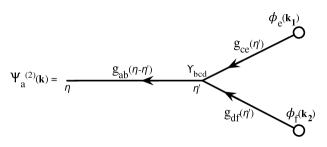
Figure 2: Diagrammatic representation of the fields at second order. This diagram value is given by Eq. (8) when one replaces ΨcsubscriptΨ𝑐\Psi_{c} and ΨdsubscriptΨ𝑑\Psi_{d} in the second term of the right hand by their linear expressions. In the diagram, each time one encounters a vertex, a time integration and a Dirac delta function in the wave modes is implicitly assumed.
Refer to caption
Figure 3: Diagrammatic representation of the fields at fifth order. Three different diagrams are found to contribute.

The computation of Gab2loopsuperscriptsubscript𝐺𝑎𝑏2loopG_{ab}^{{\rm 2-loop}} is still an arduous task that relies on the computation of many contributing terms. These terms can be formally obtained from the expression of Ψa(5)superscriptsubscriptΨ𝑎5\Psi_{a}^{(5)} that is the expression of the cosmic fields at fifth order in the initial conditions. Formally the resulting expression Ga+2loopsuperscriptsubscript𝐺limit-from𝑎2loopG_{a+}^{{\rm 2-loop}} can be written,

G1+2loop(k,η)superscriptsubscript𝐺limit-from12loop𝑘𝜂\displaystyle G_{1+}^{{\rm 2-loop}}(k,\eta) =\displaystyle= (4π)2e5ηq12dq1P0(q1)q22dq2P0(q2)(k,q1,q2)superscript4𝜋2superscript𝑒5𝜂superscriptsubscript𝑞12differential-dsubscript𝑞1subscript𝑃0subscript𝑞1superscriptsubscript𝑞22differential-dsubscript𝑞2subscript𝑃0subscript𝑞2𝑘subscript𝑞1subscript𝑞2\displaystyle(4\pi)^{2}\ e^{5\eta}\,\int q_{1}^{2}{\rm d}q_{1}\,P_{0}(q_{1})\int q_{2}^{2}{\rm d}q_{2}\,P_{0}(q_{2})\ {\cal F}(k,q_{1},q_{2}) (44)
G2+2loop(k,η)superscriptsubscript𝐺limit-from22loop𝑘𝜂\displaystyle G_{2+}^{{\rm 2-loop}}(k,\eta) =\displaystyle= (4π)2e5ηq12dq1P0(q1)q22dq2P0(q2)𝒢(k,q1,q2).superscript4𝜋2superscript𝑒5𝜂superscriptsubscript𝑞12differential-dsubscript𝑞1subscript𝑃0subscript𝑞1superscriptsubscript𝑞22differential-dsubscript𝑞2subscript𝑃0subscript𝑞2𝒢𝑘subscript𝑞1subscript𝑞2\displaystyle(4\pi)^{2}\ e^{5\eta}\,\int q_{1}^{2}{\rm d}q_{1}\,P_{0}(q_{1})\int q_{2}^{2}{\rm d}q_{2}\,P_{0}(q_{2})\ {\cal G}(k,q_{1},q_{2}). (45)

where the expressions of the functions {\cal F} and 𝒢𝒢{\cal G} can be derived from F5subscript𝐹5F_{5} and G5subscript𝐺5G_{5} respectively,

(k,q1,q2)𝑘subscript𝑞1subscript𝑞2\displaystyle{\cal F}(k,q_{1},q_{2}) =\displaystyle= 1(4π)2d2q^1d2q^2F5(𝐤,𝐪1,𝐪1,𝐪2,𝐪2),1superscript4𝜋2superscriptd2subscript^𝑞1superscriptd2subscript^𝑞2subscript𝐹5𝐤subscript𝐪1subscript𝐪1subscript𝐪2subscript𝐪2\displaystyle\frac{1}{(4\pi)^{2}}\int{\rm d}^{2}\hat{q}_{1}{\rm d}^{2}\hat{q}_{2}\ F_{5}({\bf k},{\bf q}_{1},-{\bf q}_{1},{\bf q}_{2},-{\bf q}_{2}), (46)
𝒢(k,q1,q2)𝒢𝑘subscript𝑞1subscript𝑞2\displaystyle{\cal G}(k,q_{1},q_{2}) =\displaystyle= 1(4π)2d2q^1d2q^2G5(𝐤,𝐪1,𝐪1,𝐪2,𝐪2),1superscript4𝜋2superscriptd2subscript^𝑞1superscriptd2subscript^𝑞2subscript𝐺5𝐤subscript𝐪1subscript𝐪1subscript𝐪2subscript𝐪2\displaystyle\frac{1}{(4\pi)^{2}}\int{\rm d}^{2}\hat{q}_{1}{\rm d}^{2}\hat{q}_{2}\ G_{5}({\bf k},{\bf q}_{1},-{\bf q}_{1},{\bf q}_{2},-{\bf q}_{2}), (47)

Interestingly these expressions can be represented at a diagrammatic level.

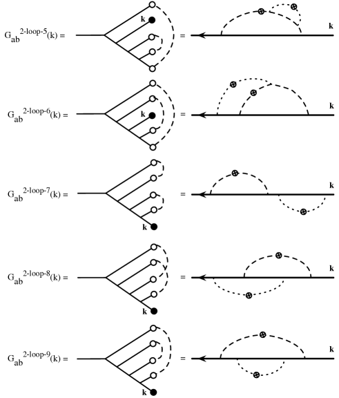
In Fig. 1 defines the linear propagator. In Fig. 2 we show how the coupling term is represented. In this diagram we show the formal expression of the second order fields. And Finally, in Fig. 3 we represent the 3 types of diagrams that contribute to the fifth order expression of the fields. It is this one that one should use to construct the two-loop contributing terms. They are obtained when 2 of the incoming lines are “glued” together: each time it introduces a linear power spectrum factor represented by a crossed circle. We are then led to the contributing diagrams depicted on Fig. 4. At this stage diagrams represent a mere transcription of the expansion of the motion equations. A detailed description of the procedure to draw the diagrams and compute their values can be found in Crocce and Scoccimarro (2006a).

Refer to caption
Refer to caption
Refer to caption
Figure 4: Diagrams contributing to the two-loop expression of the propagators.

There appear to be 9 different diagrams contributing to {\cal F} and 𝒢𝒢{\cal G}. Note that each of these diagrams comes with a symmetry factor. The computation of these symmetry factors can be done by counting the number of possibilities one has to get the same final expression out of a given contributing diagram to Ψ(5)superscriptΨ5\Psi^{(5)}. Finally the symmetry factors of the diagrams of Fig. 4 are respectively, 2,1,2,4,1,1,1,1,12124111112,1,2,4,1,1,1,1,1 for diagrams 1 to 9. Note that the diagrams contributing to the one-loop correction of the displacement field, Eq. (41), are the diagrams 1, 2 and 5 (with their previous symmetry factors) when computed in the eikonal limit.

A priori the 2 angular integrations contained in Eqs. (46-47) can be done irrespectivevely of the details of the shape of the power spectrum and can therefore be done in a model independent way. The whole computation is however cumbersome and leads to a very large number of terms, the complexity of which depends on the diagrams. Some diagrams correspond to “simple” diagram (the diagrams 1, 5, 7 and 9) the expression of which can be expressed in terms of the function f𝑓f or g𝑔g only. This is not the case however for the others. Such angular integrations involve various sets of functions. One is built out of

d2q^1|𝐤+𝐪|2=πkqlog(k+q)2(kq)2,superscriptd2^𝑞1superscript𝐤𝐪2𝜋𝑘𝑞superscript𝑘𝑞2superscript𝑘𝑞2\displaystyle\int{\rm d}^{2}\hat{q}\,\frac{1}{|{\bf k}+{\bf q}|^{2}}=\frac{\pi}{kq}\log\frac{(k+q)^{2}}{(k-q)^{2}}, (48)

and another of

d2q^1|𝐤1+𝐪|2|𝐤2𝐪|2=πlog(𝒲+/𝒲)k3q(k22q2)k12+q2(k22+k32+q2)superscriptd2^𝑞1superscriptsubscript𝐤1𝐪2superscriptsubscript𝐤2𝐪2𝜋subscript𝒲subscript𝒲subscript𝑘3𝑞superscriptsubscript𝑘22superscript𝑞2superscriptsubscript𝑘12superscript𝑞2superscriptsubscript𝑘22superscriptsubscript𝑘32superscript𝑞2\int{\rm d}^{2}\hat{q}\,\frac{1}{|{\bf k}_{1}+{\bf q}|^{2}\,|{\bf k}_{2}-{\bf q}|^{2}}=\frac{\pi\log\left(-{\cal W}_{+}/{\cal W}_{-}\right)}{k_{3}\,q\,\sqrt{\left(k_{2}^{2}-q^{2}\right)k_{1}^{2}+q^{2}\left(-k_{2}^{2}+k_{3}^{2}+q^{2}\right)}} (49)

with

𝒲±±2(k12q2)(k22q2)±4k32q2+4k3qk12k22+q4+q2(k32k12k22).subscript𝒲plus-or-minusplus-or-minusplus-or-minus2superscriptsubscript𝑘12superscript𝑞2superscriptsubscript𝑘22superscript𝑞24superscriptsubscript𝑘32superscript𝑞24subscript𝑘3𝑞superscriptsubscript𝑘12superscriptsubscript𝑘22superscript𝑞4superscript𝑞2superscriptsubscript𝑘32superscriptsubscript𝑘12𝑘superscript22\displaystyle{\cal W}_{\pm}\equiv\pm 2(k_{1}^{2}-q^{2})(k_{2}^{2}-q^{2})\pm 4k_{3}^{2}q^{2}+4k_{3}q\sqrt{k_{1}^{2}k_{2}^{2}+q^{4}+q^{2}(k_{3}^{2}-k_{1}^{2}-k2^{2})}. (50)

These two functions are those that appear in the expression of the one-loop correction to Γ(2)superscriptΓ2\Gamma^{(2)}. The calculation of {\cal F} and 𝒢𝒢{\cal G} involve however further integrals of the form,

d2q^1d2q^21|𝐪1+𝐤|2|𝐪2+𝐤|2|𝐪1+𝐪2+𝐤|2superscriptd2subscript^𝑞1superscriptd2subscript^𝑞21superscriptsubscript𝐪1𝐤2superscriptsubscript𝐪2𝐤2superscriptsubscript𝐪1subscript𝐪2𝐤2\displaystyle\int{\rm d}^{2}\hat{q}_{1}{\rm d}^{2}\hat{q}_{2}\,\frac{1}{|{\bf q}_{1}+{\bf k}|^{2}|{\bf q}_{2}+{\bf k}|^{2}|{\bf q}_{1}+{\bf q}_{2}+{\bf k}|^{2}} (51)

(for diagram 5),

d2q^1d2q^21|𝐪1+𝐪2|4|𝐪1+𝐪2+𝐤|2superscriptd2subscript^𝑞1superscriptd2subscript^𝑞21superscriptsubscript𝐪1subscript𝐪24superscriptsubscript𝐪1subscript𝐪2𝐤2\displaystyle\int{\rm d}^{2}\hat{q}_{1}{\rm d}^{2}\hat{q}_{2}\,\frac{1}{|{\bf q}_{1}+{\bf q}_{2}|^{4}|{\bf q}_{1}+{\bf q}_{2}+{\bf k}|^{2}} (52)

(for diagram 6),

d2q^1d2q^21|𝐪1+𝐪2|2|𝐪1+𝐤|2|𝐪1+𝐪2+𝐤|2,superscriptd2subscript^𝑞1superscriptd2subscript^𝑞21superscriptsubscript𝐪1subscript𝐪22superscriptsubscript𝐪1𝐤2superscriptsubscript𝐪1subscript𝐪2𝐤2\displaystyle\int{\rm d}^{2}\hat{q}_{1}{\rm d}^{2}\hat{q}_{2}\,\frac{1}{|{\bf q}_{1}+{\bf q}_{2}|^{2}|{\bf q}_{1}+{\bf k}|^{2}|{\bf q}_{1}+{\bf q}_{2}+{\bf k}|^{2}}, (53)

(for diagrams 7 and 8) or

d2q^1d2q^21|𝐪1+𝐤|2|𝐪2𝐤|2|𝐪1+𝐪2|2superscriptd2subscript^𝑞1superscriptd2subscript^𝑞21superscriptsubscript𝐪1𝐤2superscriptsubscript𝐪2𝐤2superscriptsubscript𝐪1subscript𝐪22\displaystyle\int{\rm d}^{2}\hat{q}_{1}{\rm d}^{2}\hat{q}_{2}\,\frac{1}{|{\bf q}_{1}+{\bf k}|^{2}|{\bf q}_{2}-{\bf k}|^{2}|{\bf q}_{1}+{\bf q}_{2}|^{2}} (54)

(for diagram 9). The angular integrations in those expressions can be done only partially using the relations (48, 49). We are left with expression that involve one single angle (that could indifferently be the one between 𝐪1subscript𝐪1{\bf q}_{1} and 𝐪2subscript𝐪2{\bf q}_{2} or 𝐤𝐤{\bf k} or the angle between 𝐪2subscript𝐪2{\bf q}_{2} and 𝐤𝐤{\bf k} depending on the choice of order of angle integrations). The resulting expressions are yet far too complicated to be reproduced here. In the following we rather give some general asymptotic properties and propose some fitting functions.

III.2 The asymptotic behaviors
Refer to caption
Refer to caption
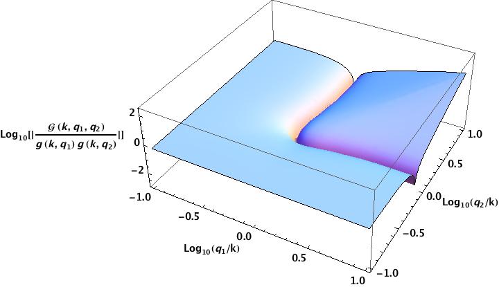
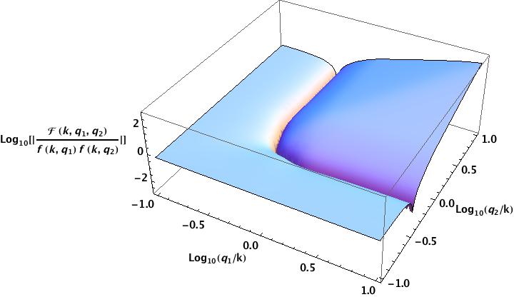
Figure 5: The functions (k,q1,q2)𝑘subscript𝑞1subscript𝑞2{\cal F}(k,q_{1},q_{2}) and 𝒢(k,q1,q2)𝒢𝑘subscript𝑞1subscript𝑞2{\cal G}(k,q_{1},q_{2}) in units respectively of f(k,q1)f(k,q2)𝑓𝑘subscript𝑞1𝑓𝑘subscript𝑞2f(k,q_{1})f(k,q_{2}) and g(k,q1)g(k,q2)𝑔𝑘subscript𝑞1𝑔𝑘subscript𝑞2g(k,q_{1})g(k,q_{2}). This illustrates the validity of the asymptotic expansions of Eq. (57).

The high k𝑘k asymptotic properties of {\cal F} and 𝒢𝒢{\cal G} can be inferred from the fact that Gab2loopsuperscriptsubscript𝐺𝑎𝑏2loopG_{ab}^{{\rm 2-loop}} should be consistent with the second order term of expression (25) in a perturbative expansion. That implies in particular that

(k,q1,q2)12k26q12k26q22.𝑘subscript𝑞1subscript𝑞212superscript𝑘26superscriptsubscript𝑞12superscript𝑘26superscriptsubscript𝑞22{\cal F}(k,q_{1},q_{2})\to\frac{1}{2}\frac{k^{2}}{6q_{1}^{2}}\frac{k^{2}}{6q_{2}^{2}}. (55)

This asymptotic property can actually be extended in a more subtle way. Let us assume that both k𝑘k and q2subscript𝑞2q_{2} are finite and that q1subscript𝑞1q_{1} is much smaller than both q2subscript𝑞2q_{2} and k𝑘k. In this case (q1,q2,k)subscript𝑞1subscript𝑞2𝑘{\cal F}(q_{1},q_{2},k) is nothing but the one-loop correction of Γ(3)superscriptΓ3\Gamma^{(3)} taken in a particular configuration. In this limit though the one-loop correction is independent on the configuration and is given by k2/(6q12)superscript𝑘26superscriptsubscript𝑞12-k^{2}/(6q_{1}^{2}) times the tree order result. As a consequences one gets a relation between {\cal F} and f𝑓f,

(k,q1,q2)k212q12f(k,q2)whenq1k and q1q2.formulae-sequence𝑘subscript𝑞1subscript𝑞2superscript𝑘212superscriptsubscript𝑞12𝑓𝑘subscript𝑞2whenmuch-less-thansubscript𝑞1𝑘 and subscript𝑞1much-less-thansubscript𝑞2{\cal F}(k,q_{1},q_{2})\to-\frac{k^{2}}{12q_{1}^{2}}f(k,q_{2})\ \ \hbox{when}\ \ q_{1}\ll k\hbox{ and }q_{1}\ll q_{2}. (56)

A similar expression naturally holds when the roles of q1subscript𝑞1q_{1} and q2subscript𝑞2q_{2} are inverted. These two results can be recapped in the following form,

(k,q1,q2)12f(k,q1)f(k,q2)whenq1k or q2k.formulae-sequence𝑘subscript𝑞1subscript𝑞212𝑓𝑘subscript𝑞1𝑓𝑘subscript𝑞2whenmuch-less-thansubscript𝑞1𝑘 or subscript𝑞2much-less-than𝑘{\cal F}(k,q_{1},q_{2})\to\frac{1}{2}f(k,q_{1})f(k,q_{2})\ \ \hbox{when}\ \ q_{1}\ll k\hbox{ or }q_{2}\ll k. (57)

Note that The validity of this approximation is controlled by the magnitude of f(k,q1)+f(k,q2)𝑓𝑘subscript𝑞1𝑓𝑘subscript𝑞2f(k,q_{1})+f(k,q_{2}). Moreover when either q1subscript𝑞1q_{1} or q2subscript𝑞2q_{2} is large one expects to obtain either a 1/q121superscriptsubscript𝑞121/q_{1}^{2} or 1/q221superscriptsubscript𝑞221/q_{2}^{2} behavior respectively. This comes from the IR properties of the kernels. All these properties can be encapsulated in the following forms,

(k,q1,q2)𝑘subscript𝑞1subscript𝑞2\displaystyle{\cal F}(k,q_{1},q_{2}) =\displaystyle= 12f(k,q1)f(k,q2)k2q12+q22αf(q1/k,q2/k),12𝑓𝑘subscript𝑞1𝑓𝑘subscript𝑞2superscript𝑘2superscriptsubscript𝑞12superscriptsubscript𝑞22subscript𝛼𝑓subscript𝑞1𝑘subscript𝑞2𝑘\displaystyle\frac{1}{2}f(k,q_{1})f(k,q_{2})-\frac{k^{2}}{q_{1}^{2}+q_{2}^{2}}\alpha_{f}(q_{1}/k,q_{2}/k), (58)
𝒢(k,q1,q2)𝒢𝑘subscript𝑞1subscript𝑞2\displaystyle{\cal G}(k,q_{1},q_{2}) =\displaystyle= 12g(k,q1)g(k,q2)k2q12+q22αg(q1/k,q2/k),12𝑔𝑘subscript𝑞1𝑔𝑘subscript𝑞2superscript𝑘2superscriptsubscript𝑞12superscriptsubscript𝑞22subscript𝛼𝑔subscript𝑞1𝑘subscript𝑞2𝑘\displaystyle\frac{1}{2}g(k,q_{1})g(k,q_{2})-\frac{k^{2}}{q_{1}^{2}+q_{2}^{2}}\alpha_{g}(q_{1}/k,q_{2}/k), (59)

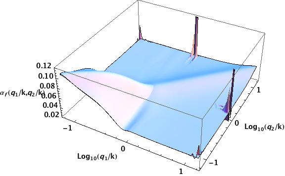
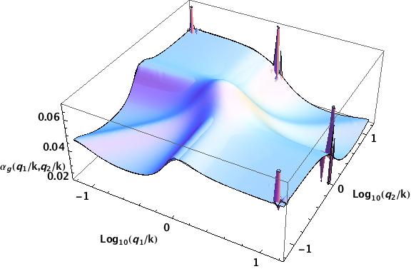
where αfsubscript𝛼𝑓\alpha_{f} and αgsubscript𝛼𝑔\alpha_{g} are both finite. The first term dominates when either q1subscript𝑞1q_{1} or q2subscript𝑞2q_{2} is small, the second when both are large. Note that the second term is always negative. This is illustrated on Fig. 5.
Refer to caption
Refer to caption
Figure 6: The functions αf(k,q1,q2)subscript𝛼𝑓𝑘subscript𝑞1subscript𝑞2\alpha_{f}(k,q_{1},q_{2}) and αg(k,q1,q2)subscript𝛼𝑔𝑘subscript𝑞1subscript𝑞2\alpha_{g}(k,q_{1},q_{2}). Each plot shows the superposition of the result of the numerical integration and the fitted functions. The results of the numerical integrations show numerical instabilities that the fitted functions do not have. The relative error between the the fitted functions and the results of the numerical integrations is less than 1% when the latter is reliable.

The functions αfsubscript𝛼𝑓\alpha_{f} and αgsubscript𝛼𝑔\alpha_{g} defined in Eqs. (58, 59) are shown on Fig. 6. They are clearly finite in all possible q1subscript𝑞1q_{1} and q2subscript𝑞2q_{2} ranges. It is actually to compute their asymptotic expressions when k𝑘k is small. They read,

αf(q1,q2)βf(q1,q2)andαg(q1,q2)βg(q1,q2)formulae-sequencesubscript𝛼𝑓subscript𝑞1subscript𝑞2subscript𝛽𝑓subscript𝑞1subscript𝑞2andsubscript𝛼𝑔subscript𝑞1subscript𝑞2subscript𝛽𝑔subscript𝑞1subscript𝑞2\alpha_{f}(q_{1},q_{2})\ \to\ \beta_{f}(q_{1},q_{2})\ \ \hbox{and}\ \ \alpha_{g}(q_{1},q_{2})\ \to\ \beta_{g}(q_{1},q_{2}) (60)

with

βf(q1,q2)subscript𝛽𝑓subscript𝑞1subscript𝑞2\displaystyle\beta_{f}(q_{1},q_{2}) =\displaystyle= (q12+q22)27518400q17q27{4q1q2(5760q110+19365q22q18114653q24q16114653q26q14+19365q28q12+5760q210)\displaystyle\frac{\left(q_{1}^{2}+q_{2}^{2}\right)}{27518400q_{1}^{7}q_{2}^{7}}\Big{\{}4q_{1}q_{2}\left(5760q_{1}^{10}+19365q_{2}^{2}q_{1}^{8}-114653q_{2}^{4}q_{1}^{6}-114653q_{2}^{6}q_{1}^{4}+19365q_{2}^{8}q_{1}^{2}+5760q_{2}^{10}\right) (61)
+15(384q14+2699q22q12+384q24)(q12q22)log4[(q1q2)2(q1+q2)2]}\displaystyle+15\left(384q_{1}^{4}+2699q_{2}^{2}q_{1}^{2}+384q_{2}^{4}\right)\left(q_{1}^{2}-q_{2}^{2}\right){}^{4}\log\left[\frac{\left(q_{1}-q_{2}\right){}^{2}}{\left(q_{1}+q_{2}\right){}^{2}}\right]\Big{\}}

and

βg(q1,q2)subscript𝛽𝑔subscript𝑞1subscript𝑞2\displaystyle\beta_{g}(q_{1},q_{2}) =\displaystyle= (q12+q22)302702400q17q27{4q1q2(17280q110+120495q22q18572759q24q16572759q26q14+120495q28q12+17280q210)\displaystyle\frac{\left(q_{1}^{2}+q_{2}^{2}\right)}{302702400q_{1}^{7}q_{2}^{7}}\Big{\{}4q_{1}q_{2}\left(17280q_{1}^{10}+120495q_{2}^{2}q_{1}^{8}-572759q_{2}^{4}q_{1}^{6}-572759q_{2}^{6}q_{1}^{4}+120495q_{2}^{8}q_{1}^{2}+17280q_{2}^{10}\right) (62)
+15(1152q14+12257q22q12+1152q24)(q12q22)log4[(q1q2)2(q1+q2)2]}.\displaystyle+15\left(1152q_{1}^{4}+12257q_{2}^{2}q_{1}^{2}+1152q_{2}^{4}\right)\left(q_{1}^{2}-q_{2}^{2}\right){}^{4}\log\left[\frac{\left(q_{1}-q_{2}\right){}^{2}}{\left(q_{1}+q_{2}\right){}^{2}}\right]\Big{\}}.

These forms are reached whenever both q1/ksubscript𝑞1𝑘q_{1}/k and q2/ksubscript𝑞2𝑘q_{2}/k are large.

In practice however the previous formulation can lead to numerical instabilities when the ratio q1/q2subscript𝑞1subscript𝑞2q_{1}/q_{2} is large. Alternative forms that make use of the expansion of the logarithm when its variable is close to unity can be employed. They are of the form,

βf(q1,q2)subscript𝛽𝑓subscript𝑞1subscript𝑞2\displaystyle\beta_{f}(q_{1},q_{2}) =\displaystyle= (q12+q22)27518400q17q27(q1+q2)4(15(q1q2)(q1+q2)4(384q14+2699q22q12+384q24)8Bν(5,0)\displaystyle\frac{\left(q_{1}^{2}+q_{2}^{2}\right)}{27518400q_{1}^{7}q_{2}^{7}\left(q_{1}+q_{2}\right){}^{4}}\left(15\left(q_{1}-q_{2}\right){}^{4}\left(q_{1}+q_{2}\right){}^{8}\left(384q_{1}^{4}+2699q_{2}^{2}q_{1}^{2}+384q_{2}^{4}\right)B_{\nu}(5,0)\right. (63)
512q15q25(2304q166144q2q15+18103q22q1450908q23q13+18103q24q126144q25q1+2304q26))\displaystyle\left.-512q_{1}^{5}q_{2}^{5}\left(2304q_{1}^{6}-6144q_{2}q_{1}^{5}+18103q_{2}^{2}q_{1}^{4}-50908q_{2}^{3}q_{1}^{3}+18103q_{2}^{4}q_{1}^{2}-6144q_{2}^{5}q_{1}+2304q_{2}^{6}\right)\right)

and

βg(q1,q2)subscript𝛽𝑔subscript𝑞1subscript𝑞2\displaystyle\beta_{g}(q_{1},q_{2}) =\displaystyle= (q12+q22)302702400q17q27(q1+q2)4(15(q1q2)(q1+q2)4(1152q14+12257q22q12+1152q24)8Bν(5,0)\displaystyle\frac{\left(q_{1}^{2}+q_{2}^{2}\right)}{302702400q_{1}^{7}q_{2}^{7}\left(q_{1}+q_{2}\right){}^{4}}\left(15\left(q_{1}-q_{2}\right){}^{4}\left(q_{1}+q_{2}\right){}^{8}\left(1152q_{1}^{4}+12257q_{2}^{2}q_{1}^{2}+1152q_{2}^{4}\right)B_{\nu}(5,0)\right. (64)
512q15q25(6912q1618432q2q15+75109q22q14235924q23q13+75109q24q1218432q25q1+6912q26))\displaystyle\left.-512q_{1}^{5}q_{2}^{5}\left(6912q_{1}^{6}-18432q_{2}q_{1}^{5}+75109q_{2}^{2}q_{1}^{4}-235924q_{2}^{3}q_{1}^{3}+75109q_{2}^{4}q_{1}^{2}-18432q_{2}^{5}q_{1}+6912q_{2}^{6}\right)\right)

where Bν(5,0)subscript𝐵𝜈50B_{\nu}(5,0) is the incomplete Beta function of index ν=4q1q2(q1+q2)2\nu=\frac{4q_{1}q_{2}}{\left(q_{1}+q_{2}\right){}^{2}}.

III.3 Fitted forms

As it is nearly impossible to reproduce the explicit result for the functions {\cal F} and 𝒢𝒢{\cal G}, we rather propose some analytical fits for αfsubscript𝛼𝑓\alpha_{f} and αgsubscript𝛼𝑔\alpha_{g} that are given below.

They can be fitted with the form (where a=f𝑎𝑓a=f or a=g𝑎𝑔a=g),

αa(q1,q2)=(βa(q1,q2)/baca(qs)da(qr))δa(qs)subscript𝛼𝑎subscript𝑞1subscript𝑞2subscript𝛽𝑎subscript𝑞1subscript𝑞2subscript𝑏𝑎subscript𝑐𝑎subscript𝑞𝑠subscript𝑑𝑎subscript𝑞𝑟subscript𝛿𝑎subscript𝑞𝑠\alpha_{a}(q_{1},q_{2})=\left(\beta_{a}(q_{1},q_{2})/b_{a}-c_{a}(q_{s})-d_{a}(q_{r})\right)\delta_{a}(q_{s})\\ (65)

where basubscript𝑏𝑎b_{a} is the value of βasubscript𝛽𝑎\beta_{a} for q1=q2subscript𝑞1subscript𝑞2q_{1}=q_{2},

bf=22382429975andbg=9886429975,formulae-sequencesubscript𝑏𝑓22382429975andsubscript𝑏𝑔9886429975b_{f}=\frac{22382}{429975}\ \ \hbox{and}\ \ b_{g}=\frac{9886}{429975}, (66)

the variable qssubscript𝑞𝑠q_{s} and qrsubscript𝑞𝑟q_{r} are defined by

qr=q12+q22andqs=1/q12+q22.formulae-sequencesubscript𝑞𝑟superscriptsubscript𝑞12superscriptsubscript𝑞22andsubscript𝑞𝑠1superscriptsubscript𝑞12superscriptsubscript𝑞22q_{r}=\sqrt{q_{1}^{2}+q_{2}^{2}}\ \ \hbox{and}\ \ q_{s}=1/\sqrt{q_{1}^{-2}+q_{2}^{-2}}. (67)

The functions ca(qs)subscript𝑐𝑎subscript𝑞𝑠c_{a}(q_{s}), da(qr)subscript𝑑𝑎subscript𝑞𝑟d_{a}(q_{r}) and δasubscript𝛿𝑎\delta_{a} are fitted functions. They are given by,

cf(qs)subscript𝑐𝑓subscript𝑞𝑠\displaystyle c_{f}(q_{s}) =\displaystyle= 0.40122835.0987qs4+4.13381qs2+11.46195qs377.7967qs6+10.40122835.0987superscriptsubscript𝑞𝑠44.13381superscriptsubscript𝑞𝑠211.46195superscriptsubscript𝑞𝑠377.7967superscriptsubscript𝑞𝑠61\displaystyle\frac{0.401228}{35.0987q_{s}^{4}+4.13381q_{s}^{2}+1}-\frac{1.46195q_{s}^{3}}{77.7967q_{s}^{6}+1} (68)
df(qr)subscript𝑑𝑓subscript𝑞𝑟\displaystyle d_{f}(q_{r}) =\displaystyle= 0.178036qr24.11634qr10+10.4258737.03063qr4+2.45787qr2+10.178036superscriptsubscript𝑞𝑟24.11634superscriptsubscript𝑞𝑟1010.4258737.03063superscriptsubscript𝑞𝑟42.45787superscriptsubscript𝑞𝑟21\displaystyle\frac{0.178036q_{r}^{2}}{4.11634q_{r}^{10}+1}-\frac{0.425873}{7.03063q_{r}^{4}+2.45787q_{r}^{2}+1} (69)
δf(qs)subscript𝛿𝑓subscript𝑞𝑠\displaystyle\delta_{f}(q_{s}) =\displaystyle= 0.0419954(76.7666qs4+4.33008qs2)76.7666qs4+1+0.01217321010.66qs4+28.3738qs2+1+0.09411180.041995476.7666superscriptsubscript𝑞𝑠44.33008superscriptsubscript𝑞𝑠276.7666superscriptsubscript𝑞𝑠410.01217321010.66superscriptsubscript𝑞𝑠428.3738superscriptsubscript𝑞𝑠210.0941118\displaystyle-\frac{0.0419954\left(76.7666q_{s}^{4}+4.33008q_{s}^{2}\right)}{76.7666q_{s}^{4}+1}+\frac{0.0121732}{1010.66q_{s}^{4}+28.3738q_{s}^{2}+1}+0.0941118 (70)
cg(qs)subscript𝑐𝑔subscript𝑞𝑠\displaystyle c_{g}(q_{s}) =\displaystyle= 0.478032qs3.28.4904qs8+10.35739142.1407qs4+1.36756qs2+10.478032superscriptsubscript𝑞𝑠328.4904superscriptsubscript𝑞𝑠810.35739142.1407superscriptsubscript𝑞𝑠41.36756superscriptsubscript𝑞𝑠21\displaystyle\frac{0.478032q_{s}^{3.}}{28.4904q_{s}^{8}+1}-\frac{0.357391}{42.1407q_{s}^{4}+1.36756q_{s}^{2}+1} (71)
dg(qr)subscript𝑑𝑔subscript𝑞𝑟\displaystyle d_{g}(q_{r}) =\displaystyle= 0.3489532.23826qr5+10.268523qr20.471174qr5+10.3489532.23826superscriptsubscript𝑞𝑟510.268523superscriptsubscript𝑞𝑟20.471174superscriptsubscript𝑞𝑟51\displaystyle\frac{0.348953}{2.23826q_{r}^{5}+1}-\frac{0.268523q_{r}^{2}}{0.471174q_{r}^{5}+1} (72)
δg(qs)subscript𝛿𝑔subscript𝑞𝑠\displaystyle\delta_{g}(q_{s}) =\displaystyle= 0.0351332(9.76583qs4+3.72325qs2)9.76583qs4+1+0.05800420.0112425qs4+2.06647qs2+10.01203980.03513329.76583superscriptsubscript𝑞𝑠43.72325superscriptsubscript𝑞𝑠29.76583superscriptsubscript𝑞𝑠410.05800420.0112425superscriptsubscript𝑞𝑠42.06647superscriptsubscript𝑞𝑠210.0120398\displaystyle\frac{0.0351332\left(9.76583q_{s}^{4}+3.72325q_{s}^{2}\right)}{9.76583q_{s}^{4}+1}+\frac{0.0580042}{0.0112425q_{s}^{4}+2.06647q_{s}^{2}+1}-0.0120398 (73)

III.4 The resulting propagators

The resulting propagators are computed with the help of the Eqs. (44, 45). The regular part of G2loopsuperscript𝐺2loopG^{{\rm 2-loop}} is then given by

Ga+2loopReg(k,η)=12[G1loopReg(k,η)]2(4π)2dq1dq2P(q1)P(q2)q12q22k2q12+q22αa(q1/k,q2/k).superscriptsuperscriptsubscript𝐺limit-from𝑎2loopReg𝑘𝜂12superscriptdelimited-[]superscriptsuperscript𝐺1loopReg𝑘𝜂2superscript4𝜋2differential-dsubscript𝑞1differential-dsubscript𝑞2𝑃subscript𝑞1𝑃subscript𝑞2superscriptsubscript𝑞12superscriptsubscript𝑞22superscript𝑘2superscriptsubscript𝑞12superscriptsubscript𝑞22subscript𝛼𝑎subscript𝑞1𝑘subscript𝑞2𝑘\displaystyle{{}^{\rm Reg}G}_{a+}^{{\rm 2-loop}}(k,\eta)=\frac{1}{2}\left[{{}^{\rm Reg}G}^{{\rm 1-loop}}(k,\eta)\right]^{2}-(4\pi)^{2}\int{{\rm d}q_{1}}\,{{\rm d}q_{2}}\,P(q_{1})\,P(q_{2})\,\frac{q_{1}^{2}\,q_{2}^{2}\,k^{2}}{q_{1}^{2}+q_{2}^{2}}\ \alpha_{a}(q_{1}/k,q_{2}/k). (74)

It is to be noted that the integrals over q1subscript𝑞1q_{1} and q2subscript𝑞2q_{2} safely converge for ΛΛ\Lambda-CDM type models. For a power spectrum that reaches a power law behavior of index n𝑛n at large k𝑘k one can easily check that the convergence is obtained for n<2𝑛2n<-2 (the condition is n<1𝑛1n<-1 for the one-loop expression). These convergence properties will be discussed in more detail in the next Section.

Finally we present the resulting shape of the propagators. At one- and two-loop level the regularized approach is un-ambiguous. It leads to,

Ga+reg1loop(k,η)=[eη+Ga+1loopReg(k,η)]exp(12k2σd2e2η).superscriptsubscript𝐺limit-from𝑎reg1loop𝑘𝜂delimited-[]superscript𝑒𝜂superscriptsuperscriptsubscript𝐺limit-from𝑎1loopReg𝑘𝜂12superscript𝑘2superscriptsubscript𝜎d2superscript𝑒2𝜂G_{a+}^{{\rm reg}-{\rm 1-loop}}(k,\eta)=\left[e^{\eta}+{{}^{\rm Reg}G}_{a+}^{{\rm 1-loop}}(k,\eta)\right]\exp\left(-\frac{1}{2}k^{2}\sigma_{\rm d}^{2}\,e^{2\eta}\right). (75)

and

Ga+reg2loop(k,η)=[eη+Ga+1loopReg(k,η)+Ga+2loopReg(k,η)]exp(12k2σd2e2η).superscriptsubscript𝐺limit-from𝑎reg2loop𝑘𝜂delimited-[]superscript𝑒𝜂superscriptsuperscriptsubscript𝐺limit-from𝑎1loopReg𝑘𝜂superscriptsuperscriptsubscript𝐺limit-from𝑎2loopReg𝑘𝜂12superscript𝑘2superscriptsubscript𝜎d2superscript𝑒2𝜂G_{a+}^{{\rm reg}-{\rm 2-loop}}(k,\eta)=\left[e^{\eta}+{{}^{\rm Reg}G}_{a+}^{{\rm 1-loop}}(k,\eta)+{{}^{\rm Reg}G}_{a+}^{{\rm 2-loop}}(k,\eta)\right]\exp\left(-\frac{1}{2}k^{2}\sigma_{\rm d}^{2}\,e^{2\eta}\right). (76)
Refer to caption
Refer to caption
Refer to caption
Refer to caption
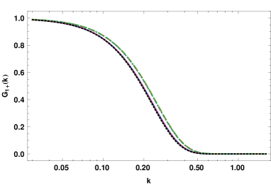
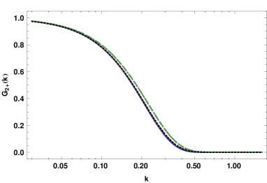
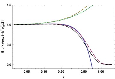
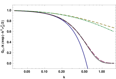
Figure 7: The resulting propagators up to two loop order in units of the linear growing mode (top) and divided by the standard damping factor (bottom). Calculations are made for a standard ΛΛ\Lambda-CDM model at z=0𝑧0z=0. The left panels correspond to the density field and the right panel to the reduced velocity divergence. The (yellow) dashed lines correspond to the RPT expression (at one loop order) and the dot-dashed lines (green) to the 1-loop regularized expression (75), the (red) long dashed lines correspond to the two-loop RPT result (78), the (blue) solid lines to the two-loop regularized expression (76) and finally the black dotted lines to the alternative form of the two-loop regularized expression obtained from (43).

We note however that it is however possible to build a RPT like expression, e.g. to exponentiate the two-loop result and construct an alternative form that contains the same two-loop order terms, At 1-loop order, the RPT propagator reads,

Ga+RPT(k,η)=eηexp(12k2σd2e2η+Ga+1loopReg(k,η)eη).superscriptsubscript𝐺limit-from𝑎RPT𝑘𝜂superscript𝑒𝜂12superscript𝑘2superscriptsubscript𝜎d2superscript𝑒2𝜂superscriptsuperscriptsubscript𝐺limit-from𝑎1loopReg𝑘𝜂superscript𝑒𝜂G_{a+}^{{\rm RPT}}(k,\eta)=e^{\eta}\,\exp\left(-\frac{1}{2}k^{2}\sigma_{\rm d}^{2}\,e^{2\eta}+{{}^{\rm Reg}G}_{a+}^{{\rm 1-loop}}(k,\eta)\,e^{-\eta}\right). (77)

This expression can be extended into,

Ga+RPT2loop(k,η)=eηexp(12k2σd2e2η+Ga+1loopReg(k,η)eη12[G1loopReg(k,η)]2eη+Ga+2loopReg(k,η)eη).superscriptsubscript𝐺limit-from𝑎RPT2loop𝑘𝜂superscript𝑒𝜂12superscript𝑘2superscriptsubscript𝜎d2superscript𝑒2𝜂superscriptsuperscriptsubscript𝐺limit-from𝑎1loopReg𝑘𝜂superscript𝑒𝜂12superscriptdelimited-[]superscriptsuperscript𝐺1loopReg𝑘𝜂2superscript𝑒𝜂superscriptsuperscriptsubscript𝐺limit-from𝑎2loopReg𝑘𝜂superscript𝑒𝜂\begin{split}G_{a+}^{{\rm RPT}-{\rm 2-loop}}(k,\eta)=e^{\eta}\,\exp\left(-\frac{1}{2}k^{2}\sigma_{\rm d}^{2}\,e^{2\eta}+{{}^{\rm Reg}G}_{a+}^{{\rm 1-loop}}(k,\eta)\,e^{-\eta}\right.\\ \left.-\frac{1}{2}\left[{{}^{\rm Reg}G}^{{\rm 1-loop}}(k,\eta)\right]^{2}\,e^{-\eta}+{{}^{\rm Reg}G}_{a+}^{{\rm 2-loop}}(k,\eta)\,e^{-\eta}\right).\end{split} (78)

This is a well-behaved expression since the second and third terms within the exponential is given by the second term of the right hand side of Eq. (58) or (59) and is negative. The resulting propagator is therefore always decreasing with k𝑘k and with time. One can remark that if αf(k,q1,q2)subscript𝛼𝑓𝑘subscript𝑞1subscript𝑞2\alpha_{f}(k,q_{1},q_{2}) and αg(k,q1,q2)subscript𝛼𝑔𝑘subscript𝑞1subscript𝑞2\alpha_{g}(k,q_{1},q_{2}) vanish the expressions Ga+RPT(k,η)superscriptsubscript𝐺limit-from𝑎RPT𝑘𝜂G_{a+}^{{\rm RPT}}(k,\eta) and Ga+RPT2loop(k,η)superscriptsubscript𝐺limit-from𝑎RPT2loop𝑘𝜂G_{a+}^{{\rm RPT}-{\rm 2-loop}}(k,\eta) are identical.

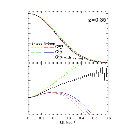
These various expressions are compared on Fig. 7. It appears that in practice, for a ΛΛ\Lambda-CDM model the one-loop expressions, (77) or (75), lead to virtually indistinguishable results in the top panels. This is also to some extent the case for the two-loop results. Differences between the one-loop and two-loop results are however significant. We will in the following compare those predictions with N-body results.

The bottom panels show more detailed comparisons of these predictions. It appears in particular that, unlike the RPT prediction at two-loop order, the Ga+2loopReg(k,η)superscriptsuperscriptsubscript𝐺limit-from𝑎2loopReg𝑘𝜂{{}^{\rm Reg}G}_{a+}^{{\rm 2-loop}}(k,\eta) form can go negative at large enough k𝑘k. This might be seen as a flaw (although this is of no consequences in practice because it takes place at scales that are quite damped) but it is corrected when one takes into account the one-loop correction to the displacement field (gray dotted lines) as it is the case when one uses Eq. (43).

We finally give below the asymptotic forms of the multi-loop corrections in the low k𝑘k limit. Formally we have

Ga+(k,η)eη+ca1loopk2e3η+ca2loopk2e5ηsubscript𝐺limit-from𝑎𝑘𝜂superscript𝑒𝜂superscriptsubscript𝑐𝑎1loopsuperscript𝑘2superscript𝑒3𝜂superscriptsubscript𝑐𝑎2loopsuperscript𝑘2superscript𝑒5𝜂G_{a+}(k,\eta)\approx e^{\eta}+c_{a}^{{\rm 1-loop}}k^{2}\,e^{3\eta}+c_{a}^{{\rm 2-loop}}k^{2}\,e^{5\eta} (79)

where

c11loop=4π61630dqP0(q),c21loop=4π313dqP0(q),formulae-sequencesuperscriptsubscript𝑐11loop4𝜋61630differential-d𝑞subscript𝑃0𝑞superscriptsubscript𝑐21loop4𝜋313differential-d𝑞subscript𝑃0𝑞c_{1}^{{\rm 1-loop}}=-4\pi\frac{61}{630}\int{\rm d}q\ P_{0}(q),\ \ c_{2}^{{\rm 1-loop}}=-4\pi\frac{3}{13}\int{\rm d}q\ P_{0}(q),\ \ (80)

according to Eqs. (33) and

ca2loop=(4π)2dq1dq2q12q22q12+q22βa(q1,q2)P0(q1)P0(q2).superscriptsubscript𝑐𝑎2loopsuperscript4𝜋2differential-dsubscript𝑞1differential-dsubscript𝑞2superscriptsubscript𝑞12superscriptsubscript𝑞22superscriptsubscript𝑞12superscriptsubscript𝑞22subscript𝛽𝑎subscript𝑞1subscript𝑞2subscript𝑃0subscript𝑞1subscript𝑃0subscript𝑞2c_{a}^{{\rm 2-loop}}=-(4\pi)^{2}\int{\rm d}q_{1}\ \int{\rm d}q_{2}\ \frac{q_{1}^{2}\ q_{2}^{2}}{q_{1}^{2}+q_{2}^{2}}\ \beta_{a}(q_{1},q_{2})\ P_{0}(q_{1})\ P_{0}(q_{2}). (81)

More specifically, for the WMAP5 cosmological parameters we have,

G1+(k,η)subscript𝐺limit-from1𝑘𝜂\displaystyle G_{1+}(k,\eta) \displaystyle\approx eηη0[1(k0.31hMpc1)2e2η2η0(k0.60hMpc1)2e4η4η0]superscript𝑒𝜂subscript𝜂0delimited-[]1superscript𝑘0.31superscriptMpc12superscript𝑒2𝜂2subscript𝜂0superscript𝑘0.60superscriptMpc12superscript𝑒4𝜂4subscript𝜂0\displaystyle e^{\eta-\eta_{0}}\left[1-\left(\frac{k}{0.31\ h{\rm Mpc}^{-1}}\right)^{2}e^{2\eta-2\eta_{0}}-\left(\frac{k}{0.60\ h{\rm Mpc}^{-1}}\right)^{2}e^{4\eta-4\eta_{0}}\right] (82)
G2+(k,η)subscript𝐺limit-from2𝑘𝜂\displaystyle G_{2+}(k,\eta) \displaystyle\approx eηη0[1(k0.17hMpc1)2e2η2η0(k0.89hMpc1)2e4η4η0]superscript𝑒𝜂subscript𝜂0delimited-[]1superscript𝑘0.17superscriptMpc12superscript𝑒2𝜂2subscript𝜂0superscript𝑘0.89superscriptMpc12superscript𝑒4𝜂4subscript𝜂0\displaystyle e^{\eta-\eta_{0}}\left[1-\left(\frac{k}{0.17\ h{\rm Mpc}^{-1}}\right)^{2}e^{2\eta-2\eta_{0}}-\left(\frac{k}{0.89\ h{\rm Mpc}^{-1}}\right)^{2}e^{4\eta-4\eta_{0}}\right] (83)

up to two-loop order where η0subscript𝜂0\eta_{0} corresponds to z=0𝑧0z=0. We note that as scales in the quasi-linear regime – say k𝑘k of the order of 0.1hMpc10.1superscriptMpc10.1h{\rm Mpc}^{-1} – the two-loop corrections induce non-negligible effects irrespectively of the shape of the damping tail one observes at high k𝑘k. This is clearly visible on the bottom panels of Fig. 7.
Refer to caption
Refer to caption
Refer to caption
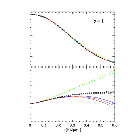
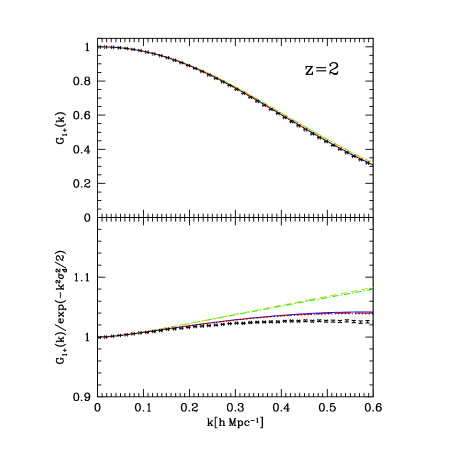
Figure 8: The regularized density propagator at 1 and 2-loop order compared to N𝑁N-body results for z=2𝑧2z=2, 111 and 0.350.350.35. The top panels correspond to the propagators in units of the linear growing factor and the bottom panels to the propagators divided by the expected leading order damping factor. The convention for the theoretical predictions are those of Fig. 7; the results from N𝑁N-body simulations are shown with black points with error-bars.

III.5 Comparisons with N-body results

Finally we compare our results with N-body measurements. Here, we briefly explain the settings of the simulations as well as how we measured the propagators.

We have performed N𝑁N-body simulations in periodic cubes with a side length of 2,048h1Mpc2048superscript1Mpc2,048h^{-1}{\rm Mpc} employing N=10243𝑁superscript10243N=1024^{3} particles. The initial conditions are created at z=15𝑧15z=15 using a parallel initial condition generator developed in Nishimichi et al. (2009); Valageas and Nishimichi (2011). The code computes the displacement field based on the second-order Lagrangian perturbation theory (2LPT; Scoccimarro (1998); Crocce et al. (2006)), and gives the displacements as well as the initial velocities to the particles placed on a regular lattice. In doing so, we adopt the best-fit flat ΛΛ\LambdaCDM cosmology to the five-year observations of WMAP satellite Komatsu et al. (2009), and compute the linear matter power spectrum by CAMB Lewis et al. (2000). We created 606060 independent realizations of particle distributions, and simulate the gravitational evolution by a publicly available tree-PM code, Gadget2. We store the outputs at z=3,2,1𝑧321z=3,2,1 and 0.350.350.35.

We assign the particles onto 10243superscript102431024^{3} grid points using the Cloud-in-Cells interpolation scheme to obtain the final density field. This field is then Fourier transformed using the Fast Fourier transformations. The propagators are measured by taking the cross correlation between this field and the linear density field. Note that here we do not use the initial particle distribution as the linear density. Instead, we employ the seed density field which has been used as the source term in the 2LPT calculation. The former suffers from a slight nonlinearity, while the latter is perfectly linear by construction.

We also perform simulations with different starting redshifts, box sizes, number of particles and internal parameters which control the force accuracy to see the convergence of the propagators. We especially pay attention to separating the effects of UV and IR cutoffs on the propagators, since we can cover only a finite wavenumber range in simulations with finite number of particles. We made sure that our box size (2,048h12048superscript12,048h^{-1} Mpc) is large enough to avoid any systematic error larger than 1%percent11\% in the propagator originating from the IR cutoff. The UV cutoff, on the other hand, can be a source of a small systematic decay of the propagator at small scale; this effect is almost independent on the output redshift, and is typically 1%percent11\% at k0.3hsimilar-to𝑘0.3k\sim 0.3h Mpc-1, and 2%percent22\% at k0.4hsimilar-to𝑘0.4k\sim 0.4h Mpc-1. The starting redshift, z=15𝑧15z=15, was chosen so that this systematic error is minimized given the box size and the number of particles; the force error (the tree force, more precisely) damps structure and leads to a stronger decay of the propagator when started at a higher redshift, while the 2LPT is no longer applicable at lower redshift. See Nishimichi et al. (in prep.) for more details.

The propagator measured from the simulations is shown as symbols in Fig. 8 with error bars showing the 111-σ𝜎\sigma uncertainties inferred from the variance among 606060 realizations. We plot Ga+(k)subscript𝐺limit-from𝑎𝑘G_{a+}(k) for the density field in the upper panels, and we also plot it after it is divided by its high-k𝑘k asymptote to make a clearer comparison. At redshifts higher than z=2𝑧2z=2, the 2-loop prediction is in good agreement with the simulation data. The N𝑁N-body data are slightly smaller than the two-loop prediction presumably due to the systematic error in the N𝑁N-body simulations (see above). On the other hand, both one-loop and two-loop predictions can not explain the N𝑁N-body data at lower redshifts (z=0.35𝑧0.35z=0.35 and and to a lesser extent z=1𝑧1z=1). The N𝑁N-body data lie in between the two predictions.

IV Convergence properties

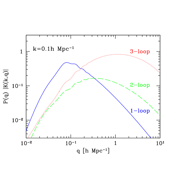
In this section, we are interested in the sensitivity of the results to the IR and UV modes. To this end, we introduce the notion of kernels that can be viewed as the response function of the propagator with respect to the initial linear spectrum. This notion is also engrained in the approach proposed in Taruya et al. (2012) to obtain accelerated computations of the non-linear power spectra. We here first properly define these quantities and explore their small and large scale behaviors.

IV.1 Monte-Carlo integrations for the three-loop contribution
Refer to caption
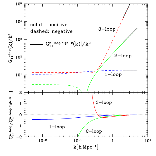
Figure 9: Monte Carlo results for G1+nloop(k)superscriptsubscript𝐺limit-from1nloop𝑘G_{1+}^{{\rm n-loop}}(k). The one-, two-, and three-loop corrections are respectively plotted as blue, green, and red lines. Top panel shows G1+nloop(k)/k2superscriptsubscript𝐺limit-from1nloop𝑘superscript𝑘2G_{1+}^{{\rm n-loop}}(k)/k^{2}, while the bottom panel shows the fractional difference of G1+nloop(k)superscriptsubscript𝐺limit-from1nloop𝑘G_{1+}^{{\rm n-loop}}(k) with its asymptotic behavior in the high k𝑘k limit G1+nloop(k)=(k2σd2/2)n/n!superscriptsubscript𝐺limit-from1nloop𝑘superscriptsuperscript𝑘2superscriptsubscript𝜎d22𝑛𝑛G_{1+}^{{\rm n-loop}}(k)=(-k^{2}\sigma_{\rm d}^{2}/2)^{n}/n! (indicated by black solid lines in top panel).
Refer to caption
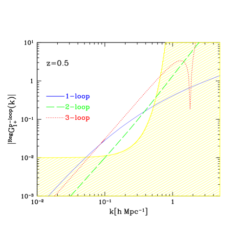
Figure 10: Regular parts of the density propagator G1+ploopReg(k)superscriptsuperscriptsubscript𝐺limit-from1ploopReg𝑘{{}^{\rm Reg}G}_{1+}^{{\rm p-loop}}(k) at one-, two-, and three-loop order with respectively solid, dashed and dotted lines. The calculations are done for z=0.5𝑧0.5z=0.5. Note that each of this contribution scales with the redshift like D+(z)2psubscript𝐷superscript𝑧2𝑝D_{+}(z)^{2p} where p𝑝p is the number of loops. The light yellow regions show the parameter space where the induced corrections to the power spectrum are less than 1 percent.

In order to gain further insights into the properties of the loop corrections, we have complemented our theoretical investigations with numerical evaluations of the three-loop contribution to the propagator. Unlike the two-loop contributions we did not try to obtain a semi-analytic expression of the results that could be used for any cosmological models. We rather aim here at evaluating the impact of the three-loop effects in a specific ΛΛ\Lambda-CDM like model.

The results we present hereafter have been obtained from brute force calculations of G1+3loopsuperscriptsubscript𝐺limit-from13loopG_{1+}^{{\rm 3-loop}}, the two-point propagator for the density starting with growing mode initial conditions. The computations focus on the calculations of the density late time propagator at z=0.5𝑧0.5z=0.5 redshift. We apply the Monte-Carlo technique of quasi-random sampling using the library Cuba555http://www.feynarts.de/cuba/, and directly perform 2D2𝐷2D, 5D5𝐷5D and 8D8𝐷8D integrations for G1+1loopsuperscriptsubscript𝐺limit-from11loopG_{1+}^{{\rm 1-loop}}, G1+2loopsuperscriptsubscript𝐺limit-from12loopG_{1+}^{{\rm 2-loop}} and G1+3loopsuperscriptsubscript𝐺limit-from13loopG_{1+}^{{\rm 3-loop}} respectively. The transfer function of the linear power spectrum is calculated with CAMB code adopting the cosmological parameters determined by WMAP5 Komatsu et al. (2009).

In Fig. 9 we separately show the one-, two-, and three-loop corrections to the two-point propagator (blue, green, and red, respectively). In top panel, to reduce the dynamic range, the results are divided by k2superscript𝑘2k^{2}, i.e., G1+nloop(k)/k2superscriptsubscript𝐺limit-from1nloop𝑘superscript𝑘2G_{1+}^{{\rm n-loop}}(k)/k^{2}, and are plotted as function of wavenumber in logarithmic scales. Note that the solid and dashed lines respectively indicate the positive and negative values in amplitude. The Monte Carlo results for one- and two-loop corrections accurately reproduce the analytic calculations. At low-k regime, all the plotted results show scale-independent behavior, indicating that the corrections behave like G1+nloop(k)k2similar-tosuperscriptsubscript𝐺limit-from1nloop𝑘superscript𝑘2G_{1+}^{{\rm n-loop}}(k)\sim k^{2}. On the other hand, at high-k regime, the three curves behave according to the expected forms described by Eq. (34). They tend to approach the asymptotic form, G1+nloop(k)=(k2σd2/2)n/n!superscriptsubscript𝐺limit-from1nloop𝑘superscriptsuperscript𝑘2superscriptsubscript𝜎d22𝑛𝑛G_{1+}^{{\rm n-loop}}(k)=(-k^{2}\sigma_{\rm d}^{2}/2)^{n}/n!, depicted as black solid lines. To see this clearly, the bottom panel of Fig. 9 shows the fractional difference between G1+nloop(k)superscriptsubscript𝐺limit-from1nloop𝑘G_{1+}^{{\rm n-loop}}(k) and its asymptotic behavior, i.e., G1+nloop(k)/[(k2σd2/2)n/n!]1superscriptsubscript𝐺limit-from1nloop𝑘delimited-[]superscriptsuperscript𝑘2superscriptsubscript𝜎d22𝑛𝑛1G_{1+}^{{\rm n-loop}}(k)/\left[(-k^{2}\sigma_{\rm d}^{2}/2)^{n}/n!\right]-1. At k1hMpc1𝑘1superscriptMpc1k\geq 1h{\rm Mpc}^{{-1}}, all the three curves consistently converge to zero. We can actually verified that the regular part of each contribution is finite at large k𝑘k.

In Fig. 10 we show the relative importance of the loop corrections as a function of scale. What is plotted are the regular parts of the terms as defined in subsection II.4. It appears that at k=0.1h/Mpc𝑘0.1Mpck=0.1h/{\rm Mpc} and at z=0.5𝑧0.5z=0.5 the one-loop contribution introduces a 5% correction, the two-loop contribution a further 2% contribution. At k=0.2h/Mpc𝑘0.2Mpck=0.2h/{\rm Mpc} the two contributions are both at 10% level but then the mode damping is already significant. Note that as the redshift is increasing the importance of all these loop corrections decreases, their magnitude scaling like D+2psuperscriptsubscript𝐷2𝑝D_{+}^{2p} where D+subscript𝐷D_{+} is the linear growth rate and p𝑝p is the number of loops.

Obviously, we hoped and expected the three-loop contribution to be smaller that the two other terms for k1h/Mpc𝑘1Mpck\leq 1h/{\rm Mpc} but this is not the case. At k=0.1h/Mpc𝑘0.1Mpck=0.1h/{\rm Mpc} it gives a 10% effect! To say the least this suggests that the three-loop corrections, assuming they are correctly evaluated by our Monte-Carlo integrations, cannot help to match the N-body results at low redshift. Given the results shown on Fig. 9 we have not much reasons to doubt the validity of the numerical integration. To better apprehend the origin of these effects we hereafter introduce the notion of kernels.

IV.2 Definitions and properties of the kernel functions

Let us define the functions Kploop(k,q)superscript𝐾ploop𝑘𝑞K^{{\rm p-loop}}(k,q) as the kernels from which the contribution of the two-point propagator to p𝑝p-loop order can be reconstructed,

Ga+ploopReg(k)=dqqKa+ploop(k,q)P0(q).superscriptsuperscriptsubscript𝐺limit-from𝑎ploopReg𝑘d𝑞𝑞superscriptsubscript𝐾limit-from𝑎ploop𝑘𝑞subscript𝑃0𝑞{{}^{\rm Reg}G}_{a+}^{{\rm p-loop}}(k)=\int\frac{{\rm d}q}{q}\ K_{a+}^{{\rm p-loop}}(k,q)P_{0}(q). (84)

We have then for instance

K1+1loop(k,q)superscriptsubscript𝐾limit-from11loop𝑘𝑞\displaystyle K_{1+}^{{\rm 1-loop}}(k,q) =\displaystyle= 4πq3(f(q,k)+16k2q2)4𝜋superscript𝑞3𝑓𝑞𝑘16superscript𝑘2superscript𝑞2\displaystyle 4\pi q^{3}\left(f(q,k)+\frac{1}{6}\frac{k^{2}}{q^{2}}\right) (85)
K1+2loop(k,q)superscriptsubscript𝐾limit-from12loop𝑘𝑞\displaystyle K_{1+}^{{\rm 2-loop}}(k,q) =\displaystyle= (4π)2q3dq1q12k2q12+q2αf(q1k,qk)P0(q1).superscript4𝜋2superscript𝑞3differential-dsubscript𝑞1superscriptsubscript𝑞12superscript𝑘2superscriptsubscript𝑞12superscript𝑞2subscript𝛼𝑓subscript𝑞1𝑘𝑞𝑘subscript𝑃0subscript𝑞1\displaystyle-(4\pi)^{2}\,q^{3}\int{{\rm d}q_{1}}\,\frac{q_{1}^{2}\,k^{2}}{q_{1}^{2}+q^{2}}\,\alpha_{f}\left(\frac{q_{1}}{k},\frac{q}{k}\right)\,P_{0}(q_{1}). (86)

Note that the kernel functions depend themselves a priori on the initial power spectrum: Ka+1loop(k,q)superscriptsubscript𝐾limit-from𝑎1loop𝑘𝑞K_{a+}^{{\rm 1-loop}}(k,q) is a tree order object, Ka+2loop(k,q)superscriptsubscript𝐾limit-from𝑎2loop𝑘𝑞K_{a+}^{{\rm 2-loop}}(k,q) a one-loop order object (and therefore a linear function of P0(q)subscript𝑃0𝑞P_{0}(q)), etc. These functions give, for each order, the impact of a linear mode q𝑞q on the amplitude of the late time mode k𝑘k we are interested in. In particular it tells how the small-scale modes affect the large-scale modes under consideration. In the following we will focus our interest in understanding the high-q𝑞q behavior of the kernel functions K(k,q)𝐾𝑘𝑞K(k,q).

Refer to caption
Figure 11: The shape of the kernel functions P0(q)K1loop(k,q)subscript𝑃0𝑞superscript𝐾1loop𝑘𝑞P_{0}(q)K^{{\rm 1-loop}}(k,q) (blue solid line), P0(q)K2loop(k,q)subscript𝑃0𝑞superscript𝐾2loop𝑘𝑞P_{0}(q)K^{{\rm 2-loop}}(k,q) (green dashed line) for k=0.1h/Mpc𝑘0.1Mpck=0.1h/{\rm Mpc} and P0(q)K3loop(k,q)subscript𝑃0𝑞superscript𝐾3loop𝑘𝑞P_{0}(q)K^{{\rm 3-loop}}(k,q) (red dotted line) as a function of q𝑞q for z=0.5𝑧0.5z=0.5.

In Fig. 11 we show the shape of the kernel functions at one, two-loop and three-loop order for k=0.1h/Mpc𝑘0.1Mpck=0.1h/{\rm Mpc}. The dashed line corresponds to the one-loop expression. As can be seen it is rather peaked at qk𝑞𝑘q\approx k and we have

K1+1loop(k,q)P0(q)superscriptsubscript𝐾limit-from11loop𝑘𝑞subscript𝑃0𝑞\displaystyle K_{1+}^{{\rm 1-loop}}(k,q)P_{0}(q) =\displaystyle= 464π315q3P0(q)forqkmuch-less-than464𝜋315superscript𝑞3subscript𝑃0𝑞for𝑞𝑘\displaystyle\frac{464\pi}{315}q^{3}P_{0}(q)\ \ {\rm for}\ q\ll k (87)
K1+1loop(k,q)P0(q)superscriptsubscript𝐾limit-from11loop𝑘𝑞subscript𝑃0𝑞\displaystyle K_{1+}^{{\rm 1-loop}}(k,q)P_{0}(q) =\displaystyle= 176π315k2qP(q)forqkmuch-greater-than176𝜋315superscript𝑘2𝑞𝑃𝑞for𝑞𝑘\displaystyle\frac{176\pi}{315}\,k^{2}\,q\ P(q)\ \ {\rm for}\ q\gg k (88)

At two-loop order, the behaviors are qualitatively different. The function peaks rather for q=0.5h/Mpc𝑞0.5Mpcq=0.5h/{\rm Mpc}, irrespectively of the value for k𝑘k (when k<0.5h/Mpc𝑘0.5Mpck<0.5h/{\rm Mpc}). We note that

K1+2loop(k,q)P0(q)k2q2P0(q)forqkformulae-sequencesimilar-tosuperscriptsubscript𝐾limit-from12loop𝑘𝑞subscript𝑃0𝑞superscript𝑘2superscript𝑞2subscript𝑃0𝑞much-greater-thanfor𝑞𝑘K_{1+}^{{\rm 2-loop}}(k,q)P_{0}(q)\sim k^{2}q^{2}P_{0}(q)\ \ {\rm for}\ q\gg k (89)

so that the convergence is obtained for a spectral index smaller than 22-2. This corresponds to the result mentioned in the beginning of subsection III.4. These trends are amplified for the three-loop results shown with a dot-dashed line for which an even lower power law index is required for convergence. In general the convergence properties of the multi-loop kernel are determined by the properties of the functions Fn(𝐪i)subscript𝐹𝑛subscript𝐪𝑖F_{n}({\bf q}_{i}) and Gn(𝐪i)subscript𝐺𝑛subscript𝐪𝑖G_{n}({\bf q}_{i}) and how they behave when one or their argument is, in norm, much larger than the sum of the wave modes. As mentioned in Scoccimarro and Frieman (1996) it is to be noted that the Galilean invariance of the motion equation implies that,

Fn(𝐪1,,𝐪n)|jqj|2qi2whenqi|jqj|,formulae-sequencesimilar-tosubscript𝐹𝑛subscript𝐪1subscript𝐪𝑛superscriptsubscript𝑗subscript𝑞𝑗2superscriptsubscript𝑞𝑖2much-greater-thanwhensubscript𝑞𝑖subscript𝑗subscript𝑞𝑗F_{n}({\bf q}_{1},\dots,{\bf q}_{n})\sim\frac{|\sum_{j}q_{j}|^{2}}{q_{i}^{2}}\ \ {\rm when}\ q_{i}\gg|\sum_{j}q_{j}|, (90)

whenever one of the qisubscript𝑞𝑖q_{i} is much larger than the sum. This can be seen at an elementary level on the properties of the vertex function α(𝐤1,𝐤2)𝛼subscript𝐤1subscript𝐤2\alpha({\bf k}_{1},{\bf k}_{2}) and β(𝐤1,𝐤2)𝛽subscript𝐤1subscript𝐤2\beta({\bf k}_{1},{\bf k}_{2}): they both vanish when the sum of the argument goes to 0. The property (90) has direct consequences on the properties of the loop corrections. As a result, the plimit-from𝑝p-loop correction takes indeed the form,

Gploop(k,η)=(4π)pq12dq1qp2dqpP0(q1)P0(qp)ploop(k,q1,,qp)superscript𝐺ploop𝑘𝜂superscript4𝜋𝑝superscriptsubscript𝑞12differential-dsubscript𝑞1superscriptsubscript𝑞𝑝2differential-dsubscript𝑞𝑝subscript𝑃0subscript𝑞1subscript𝑃0subscript𝑞𝑝superscriptploop𝑘subscript𝑞1subscript𝑞𝑝G^{{\rm p-loop}}(k,\eta)=(4\pi)^{p}\int q_{1}^{2}{\rm d}q_{1}\,\dots\,q_{p}^{2}{\rm d}q_{p}\ P_{0}(q_{1})\dots P_{0}(q_{p})\,{\cal F}^{{\rm p-loop}}(k,q_{1},\dots,q_{p}) (91)

with

ploop(k,q1,,qp)=(2p+1)!!(4π)pd2q^1d2q^pF2p+1(𝐤,𝐪1,𝐪1,,𝐪p,𝐪p)superscriptploop𝑘subscript𝑞1subscript𝑞𝑝double-factorial2𝑝1superscript4𝜋𝑝superscriptd2subscript^𝑞1superscriptd2subscript^𝑞𝑝subscript𝐹2𝑝1𝐤subscript𝐪1subscript𝐪1subscript𝐪𝑝subscript𝐪𝑝{\cal F}^{{\rm p-loop}}(k,q_{1},\dots,q_{p})=\frac{(2p+1)!!}{(4\pi)^{p}}\int{\rm d}^{2}\hat{q}_{1}\dots\rm d^{2}\hat{q}_{p}\ F_{2p+1}({\bf k},{\bf q}_{1},-{\bf q}_{1},\dots,{\bf q}_{p},-{\bf q}_{p}) (92)

where the integration is here restricted to the wave mode angles. The property (90) then implies that

ploop(k,q1,,qp)k2qi2whenqik.formulae-sequencesimilar-tosuperscriptploop𝑘subscript𝑞1subscript𝑞𝑝superscript𝑘2superscriptsubscript𝑞𝑖2much-greater-thanwhensubscript𝑞𝑖𝑘{\cal F}^{{\rm p-loop}}(k,q_{1},\dots,q_{p})\sim\frac{k^{2}}{q_{i}^{2}}\ \ {\rm when}\ q_{i}\gg k. (93)

A simple and effective way to capture this property is to write (k,q1,,qp)𝑘subscript𝑞1subscript𝑞𝑝{\cal F}(k,q_{1},\dots,q_{p}) following the functional form,

(k,q1,,qp)=k2iqi2αp(k/q1,,k/qp)𝑘subscript𝑞1subscript𝑞𝑝superscript𝑘2subscript𝑖superscriptsubscript𝑞𝑖2subscript𝛼𝑝𝑘subscript𝑞1𝑘subscript𝑞𝑝{\cal F}(k,q_{1},\dots,q_{p})=\frac{k^{2}}{\sum_{i}q_{i}^{2}}\alpha_{p}(k/q_{1},\dots,k/q_{p}) (94)

generalizing Eqs. (58,59) and where α(k/q1,,k/qp)𝛼𝑘subscript𝑞1𝑘subscript𝑞𝑝\alpha(k/q_{1},\dots,k/q_{p}) is always finite. This property determines the converging properties of the plimit-from𝑝p-loop correction to the propagator. Clearly the converging properties of the loop corrections deteriorate. It can easily be shown that formally, for a power law spectrum of index nssubscript𝑛𝑠n_{s}, the convergence is ensured only when,

ns<3+2p.subscript𝑛𝑠32𝑝n_{s}<-3+\frac{2}{p}. (95)

It clearly appears that the convergence domains shrink with the order. It leads to a greater sensitivity to the large wave-modes as one increases the loop order. What we stress here is that the kernel functions can explicitly be computed and thus one can exactly quantify the impact of large wave modes to each p𝑝p-loop correction terms.

Note that it is possible to define in general the kernel of contributing terms as

δPab(k)=dqqKab(k,q)P0(q)𝛿superscriptsubscript𝑃𝑎𝑏𝑘d𝑞𝑞superscriptsubscript𝐾𝑎𝑏𝑘𝑞subscript𝑃0𝑞\delta P_{ab}^{\sharp}(k)=\int\frac{{\rm d}q}{q}\ K_{ab}^{\sharp}(k,q)P_{0}(q) (96)

where \sharp denotes a peculiar term. One can then compare the kernels of the different terms that contribute to the non-linear power spectrum. It is worth mentioning that the kernels for the two-point propagators are the broadest. Indeed any other kernel function in the large-q𝑞q limit is going to take advantage of the asymptotic form (90) at least two times instead of one so that

K1+(k,q)P0(q)k4q4q3lP0(q)forqkformulae-sequencesimilar-tosuperscriptsubscript𝐾limit-from1𝑘𝑞subscript𝑃0𝑞superscript𝑘4superscript𝑞4superscript𝑞3𝑙subscript𝑃0𝑞much-greater-thanfor𝑞𝑘K_{1+}^{\sharp}(k,q)P_{0}(q)\sim\frac{k^{4}}{q^{4}}\ q^{3l}P_{0}(q)\ \ {\rm for}\ q\gg k (97)

where l𝑙l is the number of loops appearing in the diagram \sharp. This is to be compared with Eqs. (88, 89).

Clearly the loop corrections to the propagators are then the contributions built from perturbation theory calculations that are most sensitive to the small scale modes. At low redshift our findings imply that a regularization procedure in the UV domain should be used in order to make the contributions of these terms realistic. Unless partial resummation of higher order terms could provide us with a self-consistent regularization scheme, it should be derived from external pieces of information. This regularization could be associated for instance from the development multi-flow regimes. For instance it was advocated in Carrasco et al. (2012) that the impact of the small scale physics could be captured with an effective theory approach where effective anisotropic pressure terms are introduced in the fluid. Our results however suggest that such effects are subdominant at the one-loop order - the contributions of such terms need not be recalculated because they are naturally protected enough from UV physics - but not at two-loop order for z0.5𝑧0.5z\leq 0.5. It also suggests that when z𝑧z gets larger the importance of such corrections should vanish away even at 2 loop order at the nonlinear regime starts at larger wave-modes.

V Conclusions

Two-point propagators are key ingredients for the computation of power spectra in a cosmological context. These are also quantities for which it is easier to make analytical predictions with a Perturbation Theory approach in parts because they are expected to be damped in the large-wave modes limit in parts because the number of terms in the loop corrections are more easily computable. In this paper we have presented the most advanced results describing the expected behavior of the two-point propagators from a Perturbation Theory point of view. In particular we have exploited and extented the forms presented in Bernardeau et al. (2011) to propose theoretical expressions for the two-point propagators that incorporate up to two-loop results. The examination of these forms led to the concept of regular parts for loop contributions that are found to be finite even when the r.m.s. of the displacement field, σdsubscript𝜎d\sigma_{\rm d}, goes to infinity: regular parts are found to be the parts that contribute to the expression of the propagators once the dependence with σdsubscript𝜎d\sigma_{\rm d} has been explicitly taken into account. They also can be used as a consistency test for Monte-Carlo numerical calculations of the propagators as they predict the leading k𝑘k behavior of the contributing terms.

The main part of this paper is the explicit calculation of the two-loop contributions to the two-point propagator. We were not able to produce a simple analytical form but we rather present, in section III, simple fitting functions that capture all the expected properties of these contributions, in particular their asymptotic properties. These forms can be used for any cosmological models. Note that we propose different variants for the two-loop expression of the two-point propagator but they differ only mildly. There results are presented in Fig. 7. This is the main result of the paper. It has been compared with N𝑁N-body results. They show that two-loop corrections help significantly in predicting the shape of the two-point density propagators at z0.5𝑧0.5z\geq 0.5.

For lower redshifts the two-loop terms appear to be too large when compared to N𝑁N-body codes. We found that a possible reason for such a discrepancy is due to the increasing sensitivity of the loop corrections to the small-scale modes. A significant fraction of the contributions indeed originate from modes that are in the fully nonlinear regime. At those scales the whole perturbation theory scheme breaks down as the fluid has not only evolved into the nonlinear regime but also contains multi flow regions with order unity anisotropic pressure. The latter is not captured by the motion equations we use and should induce extra contributions as it has been put forward in recent papers, Carrasco et al. (2012); Pietroni et al. (2011). We do not think however that it has significant impact on the one-loop results. Those effects are rather expected to be significant at two-loop order and for z0.5𝑧0.5z\leq 0.5. This sensitivity to the small scale physics is shown to be stronger for the three-loop contribution that we computed with the help of Monte-Carlo integrations.

About the converging properties of the Perturbation Theory series we note that loop corrections, at any order, induce large-scale k2superscript𝑘2k^{2} corrections to the propagators and consequently to the power spectra. They are explicitly given in Eqs. (79-83) up to two-loop order with coefficients that depends on the overall shape on the linear power spectrum. Again it stresses the relative importance of the sensitivity of the standard Perturbation theory calculation to the UV domain. We also note that this sensitivity is controlled by the Galilean invariance which leads to the general property given in Eq. (90). This form appears to be a key ingredient for the converging properties of the Perturbation Theory series. It indeed sets the converging properties of both the diagrams that correspond to propagator loop corrections, as given by Eqs. (88, 89), and the other ones, as depicted in Eq. (97). Clearly if this property is dropped, the sensitivity of loop corrections to the UV domain is more severe. We note that if in standard gravity cosmologies, the relation (90) is satisfied, this is not necessarily so in cosmological models incorporating modified gravity effects or in general a clustering quintessence component. This is the case for instance in models explored in Bernardeau and Brax (2011); Chan and Scoccimarro (2009); Chuen Chan et al. (2012) that incorporate extra dynamical degrees of freedom 666This is not the case however in Sefusatti and Vernizzi (2011) in the limit that has been chosen (as indeed the coupling function α(𝐤1,𝐤2)𝛼subscript𝐤1subscript𝐤2\alpha({\bf k}_{1},{\bf k}_{2}) and β(𝐤1,𝐤2)𝛽subscript𝐤1subscript𝐤2\beta({\bf k}_{1},{\bf k}_{2}) are left unchanged).

Acknowledgements.
Numerical computations for the present work have been carried out in part on Cray XT4 at Center for Computational Astrophysics, CfCA, of National Astronomical Observatory of Japan, and in part under the Interdisciplinary Computational Science Program in Center for Computational Sciences, University of Tsukuba.
This work has been benefited from exchange visits supported by a bilateral grant from Ministère Affaires Etrangères et Européennes in France and Japan Society for the Promotion of Science (JSPS). A.T. acknowledges support from Institutional Program for Young Researcher Overseas Visit funded by the JSPS. A.T. is also supported in part by a Grant-in-Aid for Scientific Research from the JSPS (No. 24540257). T.N. is supported from the JSPS. F.B is also partly supported by the French Programme National de Cosmologie et Galaxies.

References

  • Bernardeau et al. (2011) F. Bernardeau, M. Crocce, and R. Scoccimarro, ArXiv e-prints (2011), eprint 1112.3895.
  • Eisenstein et al. (2005) D. J. Eisenstein, I. Zehavi, D. W. Hogg, R. Scoccimarro, M. R. Blanton, R. C. Nichol, R. Scranton, H.-J. Seo, M. Tegmark, Z. Zheng, et al., Astrophys. J.  633, 560 (2005), eprint arXiv:astro-ph/0501171.
  • Percival et al. (2007) W. J. Percival, R. C. Nichol, D. J. Eisenstein, D. H. Weinberg, M. Fukugita, A. C. Pope, D. P. Schneider, A. S. Szalay, M. S. Vogeley, I. Zehavi, et al., Astrophys. J.  657, 51 (2007), eprint arXiv:astro-ph/0608635.
  • Blake et al. (2011) C. Blake, T. Davis, G. B. Poole, D. Parkinson, S. Brough, M. Colless, C. Contreras, W. Couch, S. Croom, M. J. Drinkwater, et al., Mon. Not. R. Astr. Soc. 415, 2892 (2011), eprint 1105.2862.
  • Nuza et al. (2012) S. E. Nuza, A. G. Sanchez, F. Prada, A. Klypin, D. J. Schlegel, S. Gottloeber, A. D. Montero-Dorta, M. Manera, C. K. McBride, A. J. Ross, et al., ArXiv e-prints (2012), eprint 1202.6057.
  • Albrecht et al. (2006) A. Albrecht, G. Bernstein, R. Cahn, W. L. Freedman, J. Hewitt, W. Hu, J. Huth, M. Kamionkowski, E. W. Kolb, L. Knox, et al., ArXiv Astrophysics e-prints (2006), eprint arXiv:astro-ph/0609591.
  • Laureijs et al. (2011) R. Laureijs, J. Amiaux, S. Arduini, J. . Auguères, J. Brinchmann, R. Cole, M. Cropper, C. Dabin, L. Duvet, A. Ealet, et al., ArXiv e-prints (2011), eprint 1110.3193.
  • Bernardeau et al. (2002) F. Bernardeau, S. Colombi, E. Gaztañaga, and R. Scoccimarro, Phys. Rep. 367, 1 (2002).
  • Crocce and Scoccimarro (2006a) M. Crocce and R. Scoccimarro, Phys. Rev. D 73, 063519 (2006a), eprint astro-ph/0509418.
  • Taruya and Hiramatsu (2008) A. Taruya and T. Hiramatsu, Astrophys. J.  674, 617 (2008), eprint 0708.1367.
  • Pietroni (2008) M. Pietroni, J. Cosmology & Astropart. Phys. 10, 36 (2008), eprint 0806.0971.
  • Bernardeau et al. (2008) F. Bernardeau, M. Crocce, and R. Scoccimarro, Phys. Rev. D 78, 103521 (2008), eprint 0806.2334.
  • Pueblas and Scoccimarro (2009) S. Pueblas and R. Scoccimarro, Phys. Rev. D 80, 043504 (2009), eprint 0809.4606.
  • Valageas (2010) P. Valageas, ArXiv e-prints (2010), eprint 1009.0106.
  • Pietroni et al. (2011) M. Pietroni, G. Mangano, N. Saviano, and M. Viel, ArXiv e-prints (2011), eprint 1108.5203.
  • Carrasco et al. (2012) J. J. M. Carrasco, M. P. Hertzberg, and L. Senatore, ArXiv e-prints (2012), eprint 1206.2926.
  • Scoccimarro (1998) R. Scoccimarro, Mon. Not. R. Astr. Soc. 299, 1097 (1998), eprint arXiv:astro-ph/9711187.
  • Scoccimarro (2001) R. Scoccimarro, in The Onset of Nonlinearity in Cosmology, edited by J. N. Fry, J. R. Buchler, and H. Kandrup (2001), vol. 927 of New York Academy Sciences Annals, pp. 13–+.
  • Crocce et al. (2012) M. Crocce, R. Scoccimarro, and F. Bernardeau, ArXiv e-prints (2012), eprint 1207.1465.
  • Audren and Lesgourgues (2011) B. Audren and J. Lesgourgues, J. Cosmology & Astropart. Phys. 10, 037 (2011), eprint 1106.2607.
  • Crocce and Scoccimarro (2006b) M. Crocce and R. Scoccimarro, Phys. Rev. D 73, 063520 (2006b), eprint astro-ph/0509419.
  • Bernardeau et al. (2012) F. Bernardeau, N. van de Rijt, and F. Vernizzi, Phys. Rev. D 85, 063509 (2012), eprint 1109.3400.
  • Bernardeau et al. (2010) F. Bernardeau, M. Crocce, and E. Sefusatti, Phys. Rev. D 82, 083507 (2010), eprint 1006.4656.
  • Nishimichi et al. (2009) T. Nishimichi, A. Shirata, A. Taruya, K. Yahata, S. Saito, Y. Suto, R. Takahashi, N. Yoshida, T. Matsubara, N. Sugiyama, et al., Publ. Astron. Soc. Japan 61, 321 (2009), eprint 0810.0813.
  • Valageas and Nishimichi (2011) P. Valageas and T. Nishimichi, Astr. & Astrophys. 527, A87 (2011), eprint 1009.0597.
  • Crocce et al. (2006) M. Crocce, S. Pueblas, and R. Scoccimarro, Mon. Not. R. Astr. Soc. 373, 369 (2006), eprint arXiv:astro-ph/0606505.
  • Komatsu et al. (2009) E. Komatsu et al. (WMAP), Astrophys. J. Suppl. 180, 330 (2009), eprint 0803.0547.
  • Lewis et al. (2000) A. Lewis, A. Challinor, and A. Lasenby, Astrophys. J.  538, 473 (2000), eprint arXiv:astro-ph/9911177.
  • Taruya et al. (2012) A. Taruya, F. Bernardeau, T. Nishimichi, and S. Codis, ArXiv e-prints (2012), eprint 1208.1191.
  • Scoccimarro and Frieman (1996) R. Scoccimarro and J. Frieman, Astrophys. J. 473, 620 (1996), eprint astro-ph/9602070.
  • Bernardeau and Brax (2011) F. Bernardeau and P. Brax, J. Cosmology & Astropart. Phys. 6, 19 (2011), eprint 1102.1907.
  • Chan and Scoccimarro (2009) K. C. Chan and R. Scoccimarro, Phys. Rev. D 80, 104005 (2009), eprint 0906.4548.
  • Chuen Chan et al. (2012) K. Chuen Chan, R. Scoccimarro, and R. K. Sheth, ArXiv e-prints (2012), eprint 1201.3614.
  • Anselmi et al. (2011) S. Anselmi, S. Matarrese, and M. Pietroni, J. Cosmology & Astropart. Phys. 6, 15 (2011), eprint 1011.4477.
  • Sefusatti and Vernizzi (2011) E. Sefusatti and F. Vernizzi, J. Cosmology & Astropart. Phys. 3, 47 (2011), eprint 1101.1026.