Image denoising with multi-layer perceptrons, part 2:
training trade-offs and analysis of their mechanisms

Abstract

Image denoising can be described as the problem of mapping from a noisy image to a noise-free image. In Burger et al. (2012), we show that multi-layer perceptrons can achieve outstanding image denoising performance for various types of noise (additive white Gaussian noise, mixed Poisson-Gaussian noise, JPEG artifacts, salt-and-pepper noise and noise resembling stripes). In this work we discuss in detail which trade-offs have to be considered during the training procedure. We will show how to achieve good results and which pitfalls to avoid. By analysing the activation patterns of the hidden units we are able to make observations regarding the functioning principle of multi-layer perceptrons trained for image denoising.

Keywords: Multi-layer perceptrons, image denoising, training trade-offs, activation patterns

1 Introduction

In Burger et al. (2012), we show that multi-layer perceptrons (MLPs) mapping a noisy image patch to a denoised image patch are able to achieve outstanding image denoising results, even surpassing the previous state-of-the-art (Dabov et al., 2007). In addition, the MLPs outperform one type of theoretical bound in image denoising (Chatterjee and Milanfar, 2010) and come a long way toward closing the gap to a second type of theoretical bound (Levin et al., 2012). Related work in image denoising is also discussed in Burger et al. (2012). This paper explains the technical trade-offs to achieve those results.

Achieving good results with MLPs was possible through the use of larger patch sizes: It is known that larger patch sizes help make the denoising problem less ambiguous (Levin and Nadler, 2011). However, large patches also make the denoising problem more difficult (the function is higher dimensional). This required us to train high-capacity MLPs on a large number of training samples. Training such MLPs is therefore time-consuming, though modern GPUs alleviate the problem somewhat.

Training neural networks, especially large ones, is usually performed using stochastic gradient descent and is sometimes considered more of an art than a science. While there exist “tricks” to make training efficient (LeCun et al., 1998b; Bengio and Glorot, 2010), it is still quite possible that some experimental setups will lead to poor results. In these cases, it is often poorly understood why the results are bad. One might sometimes attribute these bad results to “bad luck” such as an unlucky weight initialization. This becomes a problem especially for time-consuming large-scale experiments, where multiple restarts are simply not possible. It is therefore crucial to understand which setups are likely to lead to good results and which to bad results before launching an experiment.

A common criticism regarding neural networks is that they are “black boxes”: Given a neural network, one can merely observe its output for a given input. The inner workings or logic are usually not open for inspection. Under certain circumstances, this is not the case: Convolutional neural networks (LeCun et al., 1998a) are usually easier to interpret for humans because the hidden representations can be represented as images (Lee et al., 2009). More recently, Erhan et al. (2010b) have proposed an activation maximization procedure to find an input maximizing the activation of a hidden unit, and have shown that this procedure allows for better qualitative evaluation of a network.

Contributions:

This paper aims to address the above two issues for MLPs trained to denoise image patches. In the first part of this paper, we provide a detailed description of a large and varied set of large-scale experiments. We will discuss various trade-offs encountered during the training procedure. Certain settings of training parameters can lead to initially good results, but later lead to a catastrophic degradation in performance. This phenomenon is highly undesirable and we will provide guidelines on how to avoid it, as well as an explanation of such phenomena.

In the second part of this paper, we show that surprisingly, it is possible to gain insight into the operating principle or inner workings of an MLP trained on image denoising. This is the least difficult for MLPs with a single hidden layer, but we will show that MLPs with more hidden layers are also interpretable through analysis of the activation patterns of the hidden units. We also gain insight about denoising auto-encoders (Vincent et al., 2010) due to their similarity to our MLPs.

Notation and definitions:

For an MLP with four hidden layers, each containing $2047$ hidden units, input patches of size $39\times 39$ pixels and output patches of size $17\times 17$ pixels, we use the following notation $(39\times 39,2047,2047,2047,2047,17\times 17)\equiv(39,4\times 2047,17)$. If the input and output patches are of the same size, we use the following notation $(17,4\times 2047)$ to denote an MLP with four hidden layers of size $2047$ and input and output patches of size $17\times 17$ pixels.

We will periodically halt the training procedure of an MLP and report the test performance, by which we mean the average PSNR achieved on the $11$ standard test images defined in (Burger et al., 2012). When we report the training performance, we mean the average PSNR achieved on the last $2\times 10^{6}$ training samples. The test performance therefore refers to image denoising performance, whereas the training performance refers to patch denoising performance.

2 Training trade-offs to achieve good results with MLPs

In Burger et al. (2012) we showed that it is possible to achieve state-of-the-art image denoising results with MLPs. This section will show what steps are necessary to achieve these results. We do so by tracking the evolution of the results for different experimental setups during the training process. In particular, we will vary the size of the training dataset as well as the architecture of the MLPs. We will mostly use AWG noise with $\sigma=25$. Each experiment is the result of many days and sometimes even weeks of computation time on a modern GPU (we used nVidia’s C2050).

2.1 Long training times do not result in overfitting

In this section, we will use a much smaller training set as the one defined in Burger et al. (2012). We will use the $200$ training images from the BSDS300 dataset, which is a subset of the BSDS500 dataset.

Figure 1: No overfitting even after many updates due to an abundance of training data.

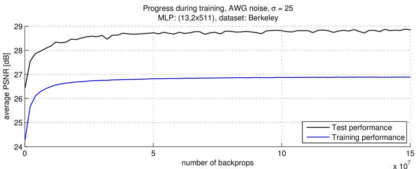
We train an MLP with architecture $(13,2\times 511)$. We report both the training performance and the test performance. The reason why the test performance is superior to the training performance is that the test performance refers to the image denoising performance (as opposed to the patch denoising performance). The image denoising performance is better than the patch denoising performance because of the averageing procedure in areas where patches overlap. We observe that the training and test performance improve steadily during the first few million updates. Results still improve after $10^{8}$ updates, albeit more slowly. On the test set, results occasionally briefly become worse. We also see that there is no overfitting even though we are using a rather small training set. This is due to the abundance of training data (the probability that a noisy patch is seen twice is zero). These results suggest that overfitting is not an issue.

2.2 Larger architectures are usually better

Figure 2: More hidden layers help. Three small hidden layers outperform one large hidden layer.

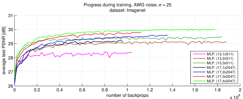
We now use the full training set—as defined in Burger et al. (2012)—and train various MLPs. The size of the patches was either $13\times 13$ or $17\times 17$. When the patch size was $13\times 13$, we used hidden layers with $511$ units. When the patch size was $17$, we used hidden layers with $2047$ units. We varied the number of hidden layers, see Figure 2.

Adding hidden layers seems to always help. Larger patch sizes and wider hidden layers seem to be beneficial. However, the MLP using patches of size $13\times 13$ and three hidden layers of size $511$ outperforms the MLP using patches of size $17\times 17$ and a single hidden layer of size $2047$.

Figure 3: More hidden layers usually help. Too many hidden layers with few hidden units cause a catastrophic degradation in performance.

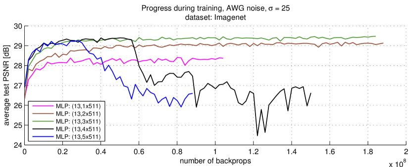
Is it always beneficial to add hidden layers?

To answer this question, we train MLPs with patches of size $13\times 13$ and hidden layers of size $511$ with four and five hidden layers, see Figure 3. The MLPs with four and five hidden layers perform well during the beginning of the training procedure, but experience a significant decrease in performance later on. The MLP achieving the best performance overall has three hidden layers. We therefore conclude that it is not always beneficial to add hidden layers.

A possible explanation for the degradation of performance shown in Figure 3 is that MLPs with more hidden layers become more difficult to learn. Indeed, each hidden layer adds non-linearities to the model. It is therefore possible that the error landscape is complex and that stochastic gradient descent gets stuck in a poor local optimum from which it is difficult to escape. In Figure 2, we see that an MLP with patches of size $17\times 17$ and four hidden layers of size $2047$ does not experience the effect shown in Figure 3, which is an indication that deep and narrow networks are more difficult to optimize than deep and wide networks.

2.3 A larger training corpus is always better

We have seen that longer training times lead to better results. Therefore, seeing more training samples helps the MLPs achieve good results.

Figure 4: Using a larger corpus of training data helps.

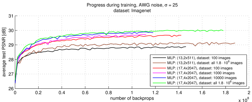
We now ask the question: What is the effect of the number of images in the training corpus? To this end, we have trained MLPs with identical architectures on training sets of different sizes, see Figure 4. We used either the full ImageNet training set or various subsets ($100$, $1000$ and $10000$ images) of the same training set. We see that significant gains can be obtained from using more training images. In particular, using even $10000$ training images delivers results that are clearly worse than results obtained when training on the full ($\sim 1.8\cdot 10^{6}$ image) training set. We also never observe a degradation in performance by using more training images.

2.4 The trade-off between small and large patches

We ask the question: Is it better to use small or large patches? We first restrict ourselves to situations where the input and output patches are of the same size.

Figure 5: Larger patches lead to better results, up to a point.

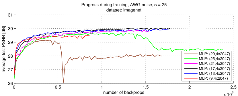
Figure 5 shows the results obtained with MLPs with four hidden layers of size $2047$ and various patch sizes. We see that up to a patch size of $17\times 17$, an increase in patch size leads to better results. This is in agreement with Levin and Nadler (2011): Using a larger support size makes the denoising problem less ambiguous.

However, increasing the patch size further leads to worse results. The results obtained using patches of size $21\times 21$ are worse than those obtained using patches of size $17\times 17$. Using patches of size $25\times 25$ leads to results that are still worse and even leads to a degradation in performance after approximately $10^{8}$ updates. For patches of size $29\times 29$ we observe still worse results and a deterioration of results after approximately $5\cdot 10^{7}$ updates. The performance later recovers slightly, but never reaches the levels achieved before the degradation in performance. For this observation, we provide an explanation similar to the one provided in section 2.2: Larger patch sizes increase the dimensionality of the problem and therefore also the difficulty. The model is therefore more difficult to optimize when large patches are used, and stochastic gradient descent may fail.

Therefore, when the input and output patches are of the same size, an ideal patch size exists (for our architectures, it seems to be approximately $17\times 17$). Patches that are too small result in a denoising function that does not deliver good results, whereas patches that are too large results in a model that is difficult to optimize.

Larger input than output patches:

What happens when we remove the restriction that the input patches be of the same size as the output patches? We expect bad results when the output patches are larger than the input patches: This would require hallucinating part of the patch. A more interesting question is: What happens when the output patches are smaller than the input patches?

Figure 6: Larger input patches help.

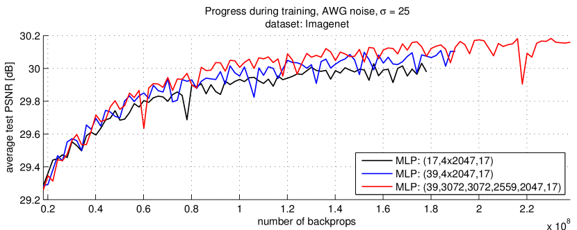
Figure 6 shows that using input patches that are larger than the output patches delivers slightly better results. Using an architecture with even more hidden units leads to even slightly better results.

Figure 7: For a given input patch size, there exists an ideal output patch size. Output patches that are too large can create problems.

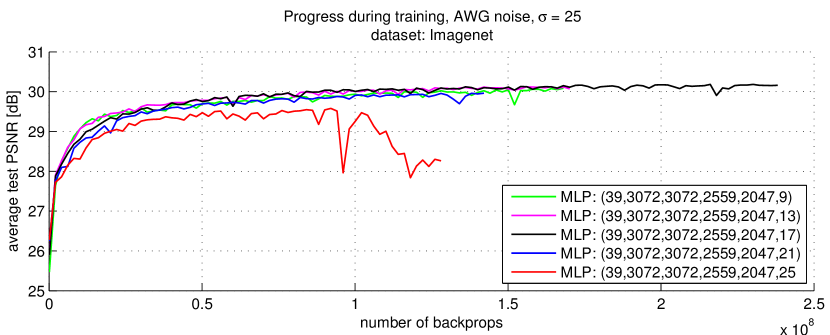
We now keep the size of the input patches fixed at $39\times 39$ pixels and vary the size of the output patches, see Figure 7. We observe that increasing the size of the output patches helps only up to a point, after which we observe a degradation in performance. The ideal output patch size seems to be the same as when the input and output patches are of the same size ($17\times 17$). Our explanation is again that output patches that are too large result in a model that is difficult to optimize.

Finally, we investigate if the patch size has an effect on the best choice of architecture.

Figure 8: Too many hidden layers combined with large output patches creates problems.

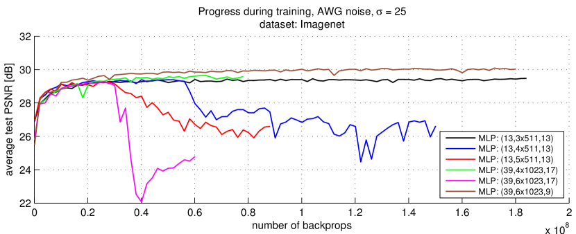
Figure 8 shows the results obtained with different patch sizes and architectures. We see again that with hidden layers of size $511$, using more than three hidden layers creates a degradation of performance when combined with patches of size $13\times 13$. With hidden layers of size $1023$, four hidden layers combined with input patches of size $39\times 39$ and output patches of size $17\times 17$, no degradation in performance is observed. Using the same patch sizes with six hidden layers of size $1023$ quickly results in a degradation in performance. However, using the same architecture, but using output patches of size $9\times 9$ results in no degradation in performance and even yields the best results in this comparison. We therefore conclude that it is the combination of deep and narrow networks combined with large output patches that are the most difficult to optimize.

Conclusions concerning MLP architectures:

We have learned that hidden layers with more units are always beneficial. Similarly, larger input patches are also always helpful. However, too many hidden layers may lead to problems in the training procedure. Problems are more likely to occur if the hidden layers contain few hidden units or if the size of the output patches is large.

2.5 Important gains in performance through “fine-tuning”

In all previous experiments, we observed that the test error fluctuates slightly. We attempt to avoid or at least reduce this behavior using a “fine-tuning” procedure: We initially train with a large learning rate and later switch to a lower learning rate. The large learning rate is supposed to encourage faster learning, whereas the low learning rate is supposed to encourage more stable results on the test data.

Figure 9: Fine-tuning improves results and reduces fluctuations in the test error. The vertical dashed line indicates where the learning rate was switched from $0.1$ to $0.001$. The two curves therefore only disagree starting at the dashed vertical line.

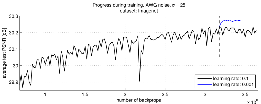
Figure 9 shows that we can indeed reduce fluctuations in the test error using a fine-tuning procedure. In addition, the switch to a lower learning rate leads to an improvement of approximately $0.05$dB on the test set. We conclude that it is important to use a fine-turning procedure to obtain good results.

2.6 Other noise variances: smaller patches for lower noise

Figure 10 shows the improvement of the test results (the average result obtained on the $11$ standard test images) during training for different values of $\sigma$. The test results achieved by the MLPs is compared against the test results achieved by BM3D. We used input patches of size $39\times 39$, output patches of size $17\times 17$ and hidden layers of sizes $3072$, $3072$, $2559$ and $2047$. We also experimented with smaller patches (“smaller patches” in Figure 10): Input patches of size $21\times 21$ and output patches of size $9\times 9$. In that case, we also used a somewhat smaller architecture: Four hidden layers of size $2047$.

Figure 10: Progress on different noise levels compared to BM3D. The higher the noise level, the faster the progress.

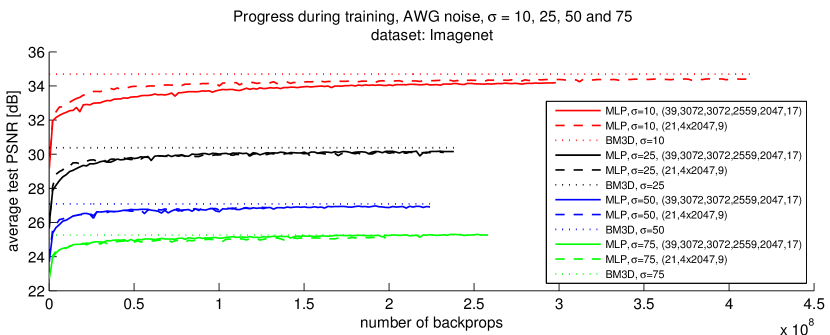
Most MLPs never reach the test results achieved by BM3D because of the relatively bad performance on image “Barbara”. For $\sigma=50$, we approach the results achieved by BM3D faster than for $\sigma=25$ and for $\sigma=25$, we approach the results achieved by BM3D faster than for $\sigma=10$. For $\sigma=75$, we approach the results achieved by BM3D the fastest and even slightly outperform the results. We see that the gap between our results and those of BM3D becomes smaller when the noise is stronger. The slower convergence for lower noise levels can be explained by the fact that the overall error is lower (or equivalently: the PSNR values are higher), which causes the updates during the training procedure to be smaller.

For $\sigma=10$, better results are achieved with smaller patches. For $\sigma=25$, $\sigma=50$ and $\sigma=75$, better results are achieved with larger patches. The reason larger patches achieve better results for $\sigma=25$, $\sigma=50$ and $\sigma=75$ is that larger patches are necessary when the noise becomes stronger (Levin and Nadler, 2011). This implies that it is not necessary to use large patches when the noise is weaker. Indeed, using patches that are too large can cause the optimization to become difficult, see section 2.4. Therefore, the ideal patch sizes are influenced by the strength of the noise. We used $21\times 21$ and $9\times 9$ patches for $\sigma=10$ and $39\times 39$ and $17\times 17$ patches for the other noise levels.

3 Training trade-offs for block-matching MLPs

We have seen in Burger et al. (2012) that MLPs can be combined with a block-matching procedure and that doing so can lead to improved results on some images. In this section, we discuss the training procedure of block-matching MLPs in more detail. We write $(39,14x13,4x2047,13)$ to denote a block-matching MLP with a search window of size $39\times 39$ pixels, taking as input $14$ patches of size $13\times 13$ pixels, four hidden layers with $2047$ hidden units each, and an output patch size of $13\times 13$ pixels.

Figure 11: Block matching helps at the beginning of the training procedure.

3.1 Block-matching MLPs can learn faster

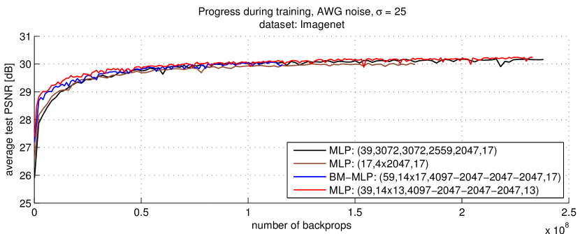
We see in Figure 11 that progress during training with the block-matching MLPs is similar to progress with the best MLPs that do not use block-matching. We see an improvement over the plain MLPs particularly at the beginning of the training procedure. Later on, the advantage of the block-matching procedure over plain MLPs is less evident. The block-matching procedure using patches of size $13\times 13$ and a search window of size $39\times 39$ performs slightly better than the block matching procedure using patches of size $17\times 17$ and a search window of size $59\times 59$. The search window size of $39\times 39$ is the same as the size of the patches the best-performing plain MLP takes as input. This means that the block-matching MLP achieving the better results always uses less information as input than the plain MLP achieving the best results, yet still achieves similar results.

Figure 12: Block matching helps particularly for image Barbara.

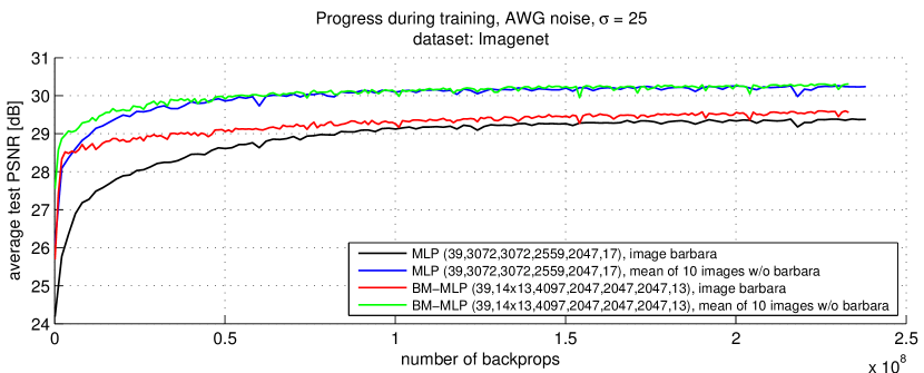
Figure 12 compares the progress of the winning plain MLP to the block-matching MLP using patches of size $13\times 13$ on image “Barbara” against the remaining $10$ of the $11$ standard test images. We see that on image “Barbara”, the block-matching MLP has a clear advantage, particularly at the beginning of the training procedure. On the remaining images, the advantage is less clear. Still, the results at the beginning of the training procedure are better for the block-matching MLP.

This answers our question: The block-matching procedure helps on images with regular structure. However, the improvement is rather small at the end of the training procedure.

3.2 Are block-matching MLPs useful on all noise levels?

We train MLPs in combination with the block matching procedure on noise levels $\sigma=10$, $\sigma=50$ and $\sigma=75$. We again use $k=14$ and patches of size $13\times 13$.

Figure 13: Progress on different noise levels compared to BM3D. Block-matching is the most useful at $\sigma=25$ and $\sigma=50$.

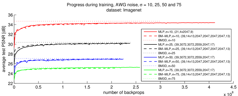
Figure 13 shows the progress during training for the different noise levels. For $\sigma=10$, the block-matching procedure seems to present no advantage over the best MLP without block-matching procedure. For $\sigma=25$ and $\sigma=50$, the block-matching procedure provides better results at the beginning of the training procedure. In the later stages of the training procedure, it is not clear if the block-matching procedure achieves superior results. For $\sigma=75$, the block-matching procedure presents no clear advantage at the beginning of the training procedure and also achieves worse results than the plain MLP in the later stages of the training procedure. A possible explanation for the deterioration of the results achieved with block-matching compared to plain MLPs at increasing noise levels is that it becomes more difficult to find patches similar to the reference patch. A possible solution would be to employ a coarse pre-filtering step such as the one employed by BM3D.

4 Analysis of hidden activation patterns

We have seen in (Burger et al., 2012) that our method can achieve good results on medium to high noise levels. We have also shown which steps are important and which are to be avoided in order to achieve good results. We now ask the question: Can we gain insight into how the MLP works? An MLP is a highly non-linear function with millions of parameters. It is therefore unlikely that we will be able to perfectly describe its behavior. This section describes a set of experiments that will nonetheless provide some insight about how the MLP works.

Definitions:

Weights connecting the input to one unit in the first hidden layer can be represented as a patch. We refer to these weights as feature detectors because they can be interpreted as filters. The weights connecting one unit in the last hidden layer of an MLP to the output can also be represented as a patch and we will refer to these as feature generators.

When feeding data into an MLP, we are interested not only in the weights, but also in the activations, by which we mean the values taken by the hidden units, due to the input. We will attempt to find inputs maximizing the activation of a specific hidden unit and refer to such an input as an input pattern. Conversely, we refer to the output caused by the activation of a single hidden unit as an output pattern.

The input pattern maximizing the activation of a hidden unit in the first hidden layer is the same as the feature detector corresponding to the hidden unit. Also, the output pattern corresponding to a hidden unit in the last hidden layer is the same as the feature generator associated to the same hidden unit.

4.1 MLPs with a single hidden layer

We start by analyzing an MLP with a single hidden layer. We use an MLP with the architecture ($17\times 17,2047,17\times 17$) for that purpose. Such an MLP is identical to a denoising auto-encoder with AWG noise (Vincent et al., 2010).

Weights as patches:

The feature detectors of this MLP can be represented as patches of size $17\times 17$ pixels. The feature generators have the same size of the feature detectors.

input

output

Figure 14: Random feature detectors (top) and the corresponding feature generators (bottom) in a trained MLP with one hidden layer.

Figure 14 shows some feature detectors (top row) and the feature generators corresponding to each feature detector (bottom row). Scaling of the pixel values was performed separately for each pair of feature detector and feature generator. The feature detectors are similar in appearance to the corresponding feature generators, up to a scaling factor. The feature detectors can be classified into three main categories: 1) feature detectors resembling Gabor filters 2) feature detectors that focus on just a small number of pixels (resembling a dot), and 3) feature detectors that look noisy. Most feature detectors belong to the first and second category. The Gabor filters occur at different scales, shifts and orientations. Similar dictionaries have also been learned by other denoising approaches. It should be noted that MLPs are not shift-invariant, which explains why some patches are shifted versions of each other. Similar features have been observed in denoising auto-encoders (Vincent et al., 2010).

feature detectors

Figure 15: Selection of feature detectors in an MLP with a single hidden layer sorted according to their standard deviation. We chose every $15$th feature detector in the sorted list. The sorting is from left to right and from top to bottom: The top-left patch has the highest standard deviation, the bottom-left patch the lowest.

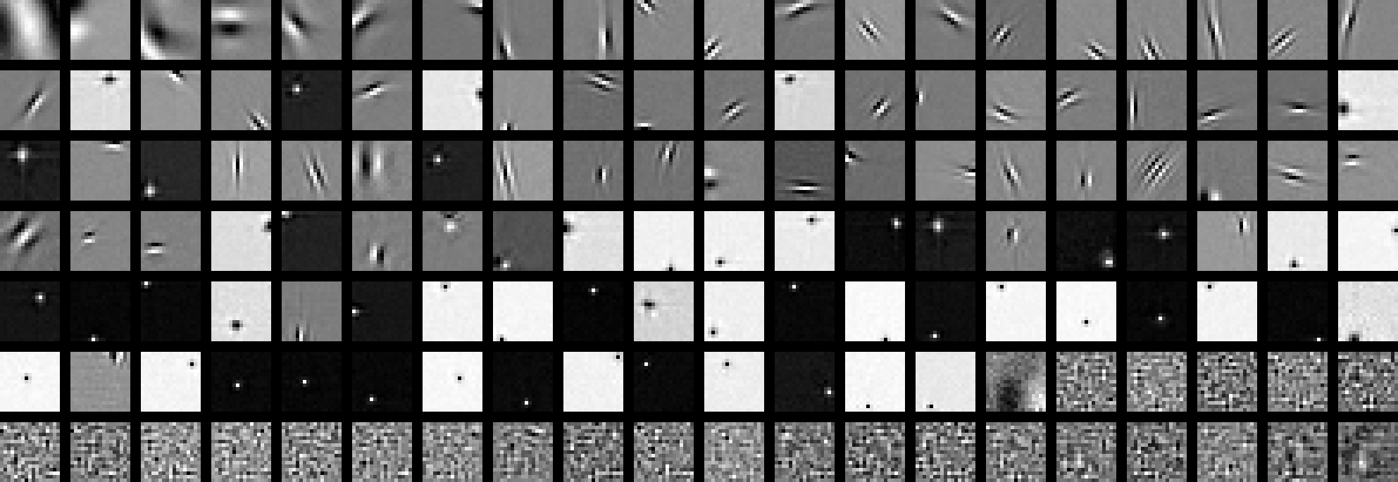
In Figure 15, the feature detectors have been sorted according to their standard deviation. We see that the feature detectors that look noisy have the lowest standard deviation. The noisy feature detectors therefore merely look noisy because of the normalization according to which they are displayed. Because the noisy-looking feature detectors have different mean values, we can interpret them as various DC-component detectors.

Denoising auto-encoders are sometimes trained with “tied” weights: The feature detectors are forced to be identical to the output bases. We observe that the learned feature detectors and feature generators look identical up to a scaling factor without the tying of the weights. This suggests that the intuition behind weight tying is reasonable. However, our observation also suggests that better results might be achieved if the feature detectors and feature generators are tied, but allowed to have different scales.

Activations:

The MLP learned a dictionary in the output layer resembling the dictionaries learned by sparse coding methods, such as KSVD. This suggests that the activations in the last hidden layer might be sparse. We therefore ask the question: What is the behavior of the activations in the hidden layer?

(a)	(b)

Figure 16: (a) Histograms of the activations in the hidden layer of a one hidden layer MLP. (b) Spectrum of the feature detectors and feature generators.

(a)	(b)

Figure 17: (a) In a trained MLP, units with small mean tend to have high entropy. This means that these units are highly active; only their mean activation is close to $0$. (b) In an untrained MLP, no units have high mean.

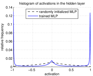
Figure 16a shows a histogram of the activations of all hidden units in both a trained MLP and a random MLP, evaluated on the $500$ images in the Berkeley dataset. The activations are centered around zero in the case of the random MLP. The activations in the trained MLP however are almost completely binary: The activations are either close to $-1$ or close to $1$, but seldom in between. This is an indication that the training process is completed: The activities lie on the saturated parts of the $\tanh$ transfer function, where the derivative is close to zero. The gradient that is back-propagated to the first layer is therefore mostly zero. This also answers our question: The activations are not sparse. We will provide a further interpretation for this observation later in this section.

Entropy:

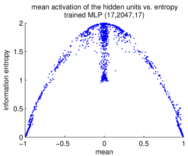
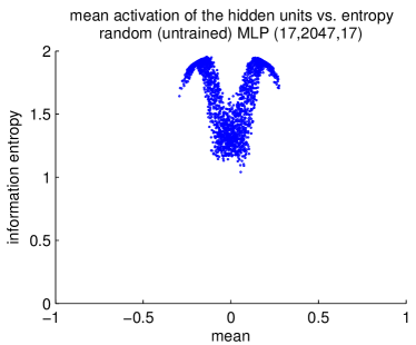
To measure the usefulness of neurons, we estimate the information entropy of their activation distributions. We plot the mean activations of hidden units against their entropy $H(X)=-\sum_{i=1}^{N}p(x_{i})\log_{2}p(x_{i})$ with four bins of equal size in Figure 17a. We repeat the experiment for an untrained MLP in Figure 17b. We see that units with high entropy tend to have a low absolute mean, and that units with low absolute mean have high entropy. The reverse is also true: units with low entropy have a high absolute mean and units with a high absolute mean have low entropy. The entropy of the units in a random MLP is higher than in a trained MLP. This is explained by the fact that the random MLP has no units with high absolute mean. These observations allow us to conclude that the units that have a mean close to $0$ also have a binary behavior: They are either $1$ or $-1$ and seldom have a value in between. In fact, we can say that these units take value $1$ in approximately $50\%$ of the cases and value $-1$ in the remaining cases. They therefore have a high entropy.

feature detectors

feature detectors

Figure 18: Feature detectors of the units with the highest (top) and lowest (bottom) entropy.

Figure 18 shows the feature detectors of the units with the highest and lowest entropy. The feature detectors with the lowest entropy all resemble high-frequency Gabor filters of different positions and orientations. A possible explanation for their low entropy is that these filters are highly selective. Only few patches cause these filters to activate.

Weight spectrum:

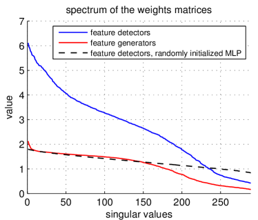
We perform an SVD-decomposition of the weight matrices of both the trained and the random MLP and plot the spectrum of the singular values, see Figure 16b. For the random MLP, we omit the spectrum of the feature generators because its shape is identical to the spectrum of the feature detectors. This is due to the initialization procedure and symmetrical architecture.

The similar shape of the spectra in the trained MLP was expected: the feature detectors and feature generators are similar in appearance, see Figure 14. The larger singular values for the feature detectors is a reflection of the fact that the norms of the feature detectors is larger than the norm of the feature generators (also seen in Figure 14).

The spectrum for both the feature detectors and the feature generators is relatively flat, which is an indication that the feature detectors are diverse: Strong correlations between feature detectors would cause small singular values. The fact that there are no singular values with value zero means that the output bases matrix has full rank. The spectrum of the random MLP is even flatter: it also has full rank. This means that the output bases of both the trained and the random MLP are able to approximate any patch.

(a)	(b)

Figure 19: (a) Many hidden units are strongly correlated when image data is given as input. (b) The hidden units are not strongly correlated when noise is given as input.

Activation correlations:

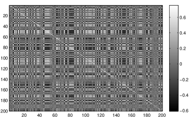
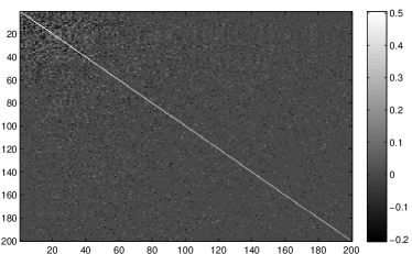
Figure 19a shows the covariance matrix between the $200$ hidden units of the trained MLP with the highest variance, when image data is provided as input. We see that activations between units are highly correlated. This is a reflection of the fact that many of the features detected by the filters tend to occur simultaneously in image patches. Figure 19b shows that this observation does not hold when noise is provided as input.

(a)	(b)

Figure 20: (a) Applying a squashing function on a normally distributed vector with high variance creates a binary distribution. (b) AWG noise with $\sigma=25$ will cause mostly binary activations in the hidden layer.

How do the binary codes arise?

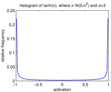
We observed in Figure 16a that the codes in the hidden layer are almost completely binary. This observation is surprising: The binary distribution was not explicitly enforced and the distribution of activations is usually different (Bengio and Glorot, 2010). A possible explanation would be if the activities prior to the application of the $\tanh$-function have high variance. Applying the $\tanh$-function on a normally-distributed vector with high variance indeed creates a binary distribution, see Figure 20a.

Is this explanation plausible? A supporting argument is that the feature detectors shown in Figure 14 have high norm compared to their corresponding output bases. The high norm of the filters could cause high activations in the hidden layers.

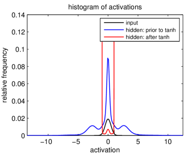
We now feed AWG noise with $\sigma=25$ into the MLP. The histograms of the activations prior and after application of the $\tanh$-layer are shown in Figure 20b. We observe that the activations before the $\tanh$-layer indeed have high variance and that the activations after the $\tanh$-layer are indeed mostly binary. We conclude that the binary activities in the hidden layer are due to activities with high variance prior to the $\tanh$-layer, which are in turn due to feature detectors with high norm.

Figure 21: The $\tanh$-layer has a denoising effect due to saturation.

Figure 22: Denoising in action: The input maximizes the activity of one feature detector (hidden neuron). Other feature detectors are also strongly activated. After the $\tanh$-layer, the noise has almost no effect on the feature detectors that are highly active. The activations in b) are sorted and the activations in c) use the same sorting. Denoising happens mostly in the blue areas in c).

Figure 23: Denoising through hard-thresholding: Setting the less import feature detectors to $0$ also produces a denoising effect. The activations in b) are sorted and the activations in c) use the same sorting.

How is denoising achieved?

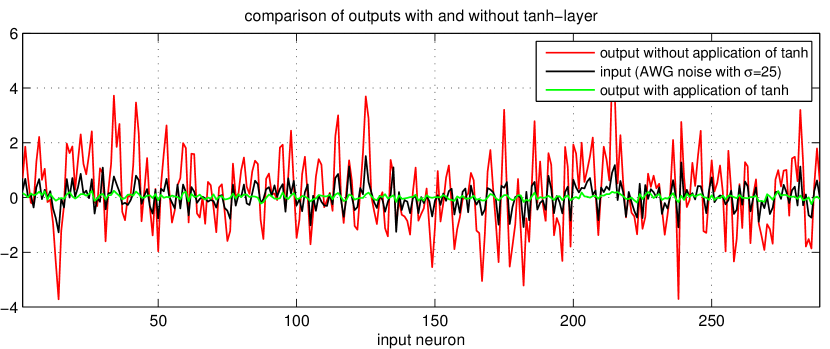
We have made a number of observations regarding the behavior of the MLP but have not yet explained why the MLP is able to denoise. Is the binarization effect observed in Figure 20 an important factor? To answer this question, we feed an image patch containing only AWG noise with $\sigma=25$ through the MLP. We compare the output when the $\tanh$-layer is applied to when the $\tanh$-layer is not applied, see Figure 21. Without $\tanh$-layer, the output is more noisy than the input. With $\tanh$-layer however, the output is less noisy than the input. We can therefore conclude that the same thresholding operation responsible for the binary codes is also at least partially responsible for the denoising effect of the MLP.

Thresholding for denoising has been thoroughly studied and dates back at least to “coring” for reducing television noise (Rossi, 1978). Typically, a thresholding operation is performed in some transform domain, such as a wavelet domain (Portilla et al., 2003). However, the thresholding operations typically affect small values most strongly: In the case of hard thresholding, values close to zero are set to zero and all other values are left unchanged. In the case of soft thresholding, all values are reduced by a fixed amount. Then, values close to zero are set to zero. In the MLP, the situation is reversed: Values close to zero are left unchanged. Only large absolute values are modified by the $\tanh$-layer. We call this effect saturation.

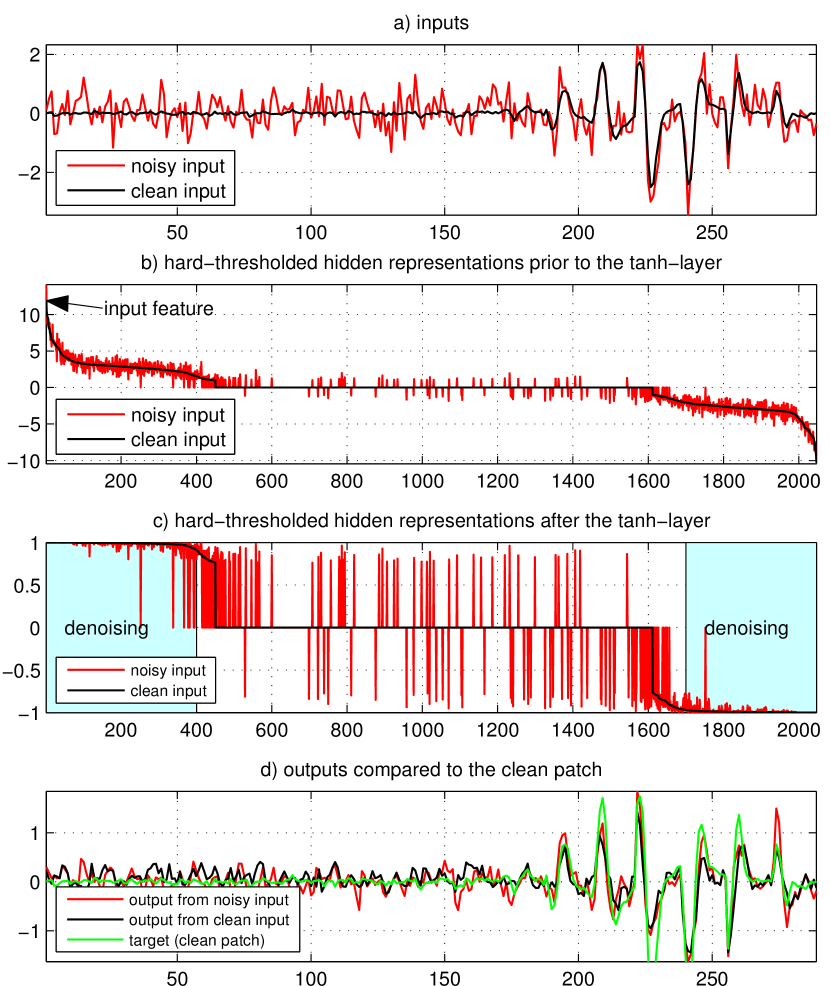
We have seen that the saturation of the $\tanh$-layer can explain why noise is reduced. However, denoising can always be trivially achieved by removing both noise and image information. We therefore ask the question: Why are image features preserved? We proceed by example. As input, we will use the feature detected by one of the feature detectors. As a comparison, we will use as input a noisy version of this feature, see Figure 22a. The clean input has the effect of maximizing the activity of its corresponding feature detector prior to the $\tanh$-layer, see Figure 22b. Other feature detectors also have a high value, which should be expected, given the high covariance of the hidden units, see Figure 19. We see that the noisy input creates a hidden representation that looks quite different from the one created from the clean input: The noise is still clearly present. After application of the $\tanh$-layer, the noise is almost completely eliminated on the feature detectors with high activity, see Figure 22c. This is due to the saturation of the $\tanh$-layer. The outputs look similar to the clean input, see Figure 22d. In particular, the noise from the noisy input has been attenuated.

We repeat the experiment performed in Figure 22, but this time hard-threshold the hidden activities: Activities in the hidden layer prior to the $\tanh$-layer with an absolute value smaller than $1$ are set to $0$. Doing so still produces a denoising effect, see Figure 23. This observation brings us to the conclusion that the feature detectors with a high activity are the more important ones. This is convenient, because the noise on the feature detectors with high activities disappears due to saturation.

We summarize the denoising process in a one-hidden-layer MLP as follows. Noise is attenuated through the saturation of the $\tanh$-layer. Image features are preserved due to the high activation values of the corresponding feature detectors.

Relation to stacked denoising autoencoders (SDAEs):

MLPs with a single hidden-layer which are trained on the denoising task are exactly equivalent to denoising autoencoders. Denoising autoencoders can be stacked into SDAEs (Vincent et al., 2010). The difference between SDAEs and MLPs with multiple hidden layers is that SDAEs are trained sequentially: One layer is trained at a time and each layer is trained to denoise the output provided by the previous layer (or the input data in the case of the first layer). While our MLPs are trained to optimize denoising performance, SDAEs are trained to provide a useful initialization for a different supervised task.

It has been suggested by Bengio et al. (2007) that deep learning is useful due to an optimization effect: Greedy layer-wise training helps to optimize the training criterion. However, later work contradicts this interpretation: Erhan et al. (2010a) suggest that SDAEs and other deep pre-trained architectures such as deep belief nets (DBNs) are useful due to a regularization effect: Supervised training of an architecture (especially a deep one) using stochastic gradient descent is difficult because of an abundance of local minima, many of them poor (in the sense that they do not generalize well). The unsupervised pre-training phase imposes a restriction on the regions of parameter space that stochastic gradient descent can explore during the supervised phase and reduces the number of local minima that stochastic gradient descent can fall into. Pre-training thus initializes the architecture in such a way that stochastic gradient descent finds a better basin of attraction (again in the sense of generalization).

The fact that activations in the hidden layers of a SDAE are almost completely binary (see Figure 16) and relatively high entropy (see Figure 17a) was not mentioned by Erhan et al. (2010a), but is in agreement with the regularization interpretation: The fact that the denoising task forces the hidden representations to be binary is a restriction and therefore also a form of regularization. In addition, information about the input should be preserved in order for the hidden representations to be useful. Information about the input is preserved by virtue of the denoising task: The hidden representations have to contain sufficient information to reconstruct the uncorrupted input. The fact that the hidden units have relatively high information entropy is an additional indication that information is preserved.

We have not answered the question if the binary restriction is better than a more classical form of regularization, such as $\ell_{1}$ or $\ell_{2}$ regularization. However, Erhan et al. (2010a) suggest that pre-training achieves a form of regularization that is different from and indeed more useful than $\ell_{1}$ or $\ell_{2}$ regularization on the parameters ($\ell_{2}$ regularization on the weights is approximately equivalent to $\ell_{2}$ regularization on the activations). Another argument is that binary vectors are easier to manipulate (e.g. classify) than vectors with small norm.

Relation to restricted Boltzmann machines and deep belief nets:

The binary activations in the hidden layer of our MLP are reminiscent of restricted boltzmann machines (RBMs) and deep belief nets (DBNs), which usually employ stochastic binary activations during the unsupervised training phase (Hinton et al., 2006). An additional similarity is that it has been shown that DBNs and stacked denoising autoencoders extract similar features when trained on either hand-written digits or natural image patches (Erhan et al., 2010b).

feature detectors in an RBM

Figure 24: Some filters learned by an RBM trained on natural image data (in an unsupervised fashion) with Gaussian visible units, patches of size $17\times 17$ and $512$ stochastic binary hidden units. The filters resemble those learned by an MLP on the denoising task.

We trained an RBM with Gaussian visible units on image patches of size $17\times 17$ using contrastive divergence (Hinton, 2002, 2010). Figure 24 shows that the filters learned by the RBM are similar in appearance to the filters learned by our one-hidden layer MLP, which is in agreement with the findings of Erhan et al. (2010b).

(a)	(b)

Figure 25: (a) Histogram of activations in the hidden layer of an RBM trained in an unsupervised fashion on natural image patches. (b) Histogram of activations in the hidden layers of a DBN trained in an unsupervised fashion on handwritten digits (Hinton and Salakhutdinov, 2006).

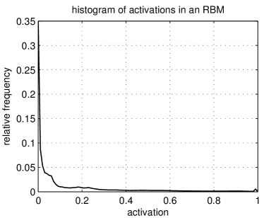
The activations of the RBM are binary and stochastic during the unsupervised pre-training phase. It is possible to use the weights learned during pre-training for a supervised task, in which case the hidden units are allowed to take real values. After unsupervised learning of our RBM, we observe the distribution of the real-valued activations in the hidden layer, see Figure 25a. The activations lie between $0$ and $1$ instead of between $-1$ and $1$ for our MLP because of the use of the logistic function instead of $\tanh$. We see that the activations are sparse and do not show the binary behavior exhibited by our MLP.

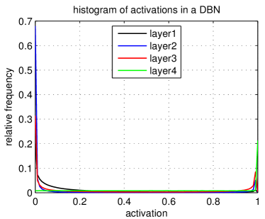
We also used the code provided by Hinton and Salakhutdinov (2006) to train a deep belief net (DBN) on hand-written digits. After pre-training, the activation in all layers is also sparse, see Figure 25b. We see that sparsity occurs in the hidden layers even when not explicitly enforced, as proposed by Hinton (2010).

Summary:

MLPs with one hidden layer denoise by detecting features in the noisy input patch. Each feature detector responds maximally to a single feature, but usually many features are detected simultaneously (see Figure 19). The denoised output corresponds to a weighted sum of each feature detector, see Figure 14, where the weight depends on the response of the feature detector. The features are mostly Gabor filters of different scales, locations and orientations. Similar features are observed when training other models on natural image data, such as RBMs, see Figure 24. The features are informative in the sense that many hidden units have high information entropy, see Figure 17b. Noise is removed through saturation of the $\tanh$-layer. Saturation is achieved through feature detectors with high norm, which in turn leads to activations with high variance in the hidden layer before the $\tanh$-layer and mostly binary activations after the $\tanh$-layer, see Figure 20. The binary distribution of activations is surprising given the fact that it has not been explicitly enforced, but is useful for denoising and also fits well into the regularization interpretation of denoising auto-encoders proposed by Erhan et al. (2010a).

4.2 MLPs with several hidden layers

The behavior of MLPs with a single hidden layer is easily interpretable. However, we have seen in Section 2.2 that MLPs with more hidden layers achieve better results. Unfortunately, interpreting the behavior of an MLP with more hidden layers is more complicated. The weights in the input layer and in the output layer can still be represented as image patches, but the layer or layers between the input and output are not so easy to interpret. MLPs with a single hidden layer are identical to denoising autoencoders. This is not true anymore for MLPs with more hidden layers.

feature detectors

feature generators

Figure 26: Random selection of weights in the input layer (top) and output layer (bottom) for an MLP with two hidden layers.

Two hidden layers:

We will start by studying an MLP with architecture ($17\times 172$, $2047$, $2047$,$17\times 172$). We repeat the experiment we performed on an MLP with a single hidden layer and look at the feature detectors and feature generators of the MLP, see Figure 26. We notice that the feature generators look relatively similar to the output bases of the MLP with a single hidden layer. However, the feature detectors now look different: Many look somewhat noisy (perhaps resembling grating filters) or seem to extract a feature that is difficult to interpret. Intuition would suggest that these filters are in some sense worse than those learned by the single hidden layer MLP. However, we have seen in Figure 2 that better results are achieved with the MLP with two hidden layers than with one hidden layer.

feature detectors

feature generators

Figure 27: Random selection of weights in the input layer (top) and output layer (bottom) for an MLP with four hidden layers.

Four hidden layers:

We look at the feature detectors and the output bases of an MLP with architecture ($17\times 17$, $2047$, $2047$, $2047$, $2047$, $17\times 17$), see Figure 27. The output bases resemble those of the MLPs with one and two hidden layers. The feature detectors however look still noisier than those of the MLP with two hidden layers. The results achieved with the MLP with four hidden layers are again better than those achieved with a two hidden layer MLP, see Figure 2. We conclude that feature detectors that look noisy or are just difficult to interpret do not necessarily lead to worse denoising results.

feature detectors

output patterns

Figure 28: Feature detectors (top) and outputs (bottom) corresponding to each feature detector, using an MLP with two hidden layers. The detection of one feature causes the generation of a similar feature in the output.

feature detectors

output patterns

Figure 29: Feature detectors (top) and outputs (bottom) corresponding to each feature detector, using an MLP with four hidden layers. The detection of one feature causes the generation of a similar feature in the output.

Outputs corresponding to feature detectors:

In the MLP with a single hidden layer, there was a clear correspondence between feature detectors and feature generators: The feature generators looked identical to their corresponding feature detectors. This correspondence is lost in MLPs with more hidden layers, due to the additional hidden layer separating feature detectors from output bases. Can we still find a connection between feature detectors and corresponding outputs? To answer this question, we activate a single unit in the first hidden layer: The unit is assigned value $1$ and all other units are set to $0$. We then perform a forward pass through the MLP, but completely ignore the input of the MLP. Doing so provides us with an tentative answer to the question: What output is caused by the detection of one feature? The answer is only tentative because several features are usually detected simultaneously. The activation of more hidden units can cause additional non-linear effects due to the $\tanh$-functions in the MLP. Figure 28 and 29 show the outputs obtained with an MLP with two and four hidden layers, respectively. Also shown are the feature detectors corresponding to the hidden units causing the outputs. We observe a similar correspondence between feature detectors and outputs as in the case of a single hidden layer MLP. The effect is more visible with the MLP with two hidden layers than with the MLP with four hidden layers. The fact that the outputs do not perfectly correspond to their feature detectors can be explained by the fact that during training, features are never detected separately, but always in combination with other features.

input patterns

feature generators

Figure 30: Features discovered through activation maximization (top) and corresponding feature generators (bottom), using an MLP with two hidden layers. The detection of one feature causes the generation of a similar feature in the output.

input patterns

feature generators

Figure 31: Features discovered through activation maximization (top) and corresponding feature generators (bottom), using an MLP with four hidden layers. The detection of one feature causes the generation of a similar feature in the output.

Inputs maximally activating single output bases:

Which inputs cause the highest activation for each hidden neuron? Answering this question should tell us which features the MLP responds to. We answer this question using activation maximization, proposed by Erhan et al. (2010b). Activation maximization is a gradient-based technique for finding an input maximizing the activation of a neuron. We use activation maximization with a step size of $0.1$. We initialize the patches with samples drawn from a normal distribution with mean $0$ and unit variance. We limit the norm of the patch to the norm of the initial patch.

We apply activation maximization on neurons in the last hidden layer of the MLPs with two and four hidden layers. The procedure indeed finds interesting features, see Figures 30 and 31. Even more interesting is the fact that the features found through activation maximization bear a strong resemblance to the feature generators connected to the same hidden neuron.

input patterns

output patterns

Figure 32: Input patterns discovered through activation maximization (top) and output patterns created using one active unit in the hidden layer (bottom), using an MLP with four hidden layers. We used the third hidden layer. We see a correspondence between the input and output patterns.

Input patterns vs. output patterns:

We also observe a correspondence between the input patterns discovered through activation maximization and output patterns created by activating a single hidden neuron in deeper layers. Figure 32 demonstrates this correspondence in the third hidden layer of an MLP with four hidden layers.

Summary:

MLPs with more hidden layers tend to have feature detectors that are not easily interpretable. In fact, one might be tempted to conclude that they are inferior in some way to the feature detectors learned by an MLP with a single hidden layer, because many of the feature detectors look noisy. However, the denoising results obtained with MLPs with more hidden layers is superior. The visual appearance of the feature detectors is therefore not a disadvantage. The better denoising results can be explained by the higher capacity of MLPs with more hidden layers. MLPs with more hidden layers also seem to operate according to the same principle as MLPs with a single hidden layer: If a feature is detected in the noisy patch, a weighted version of the feature is added to the denoised patch.

4.3 MLPs with larger inputs

We now consider the MLP that provided the best results on AWG noise with $\sigma=25$, see Figure 2. The MLP has architecture ($39\times 39$, $3072$, $3072$, $2559$, $2047$, $17\times 17$). The main difference between this MLP and the previous ones is that the input patches are larger than the output patches. An additional difference is the somewhat larger architecture.

feature detectors

feature generators

Figure 33: Random selection of weights in the input layer (top) and output layer (bottom) of the MLP providing the best results: $(39,3072,3072,2559.2047,17)$. This MLP has input patches of size $39\times 39$ and output patches of size $17\times 17$.

Feature detectors and feature generators:

Figure 33 shows a set of feature detectors and feature generators for the MLP with larger input patches. The feature generators look similar to those learned by other MLPs. However, the feature detectors again look somewhat different: many seem to focus on the center area of the input patch. In addition, many look noisy. The fact that many feature detectors focus on the center area of the input patch can be explained by the fact that the output patches are smaller than the input patches. The target patches correspond to the center region of the input patches. Correlations between pixels fall with distance, which implies that the pixels at the outer border of the input patch should be the least important for denoising the center patch.

(a)	(b)

Figure 34: (a) Histograms of the activations in the last hidden layer. (b) Histograms of the activations in the first three hidden layers.

Activations:

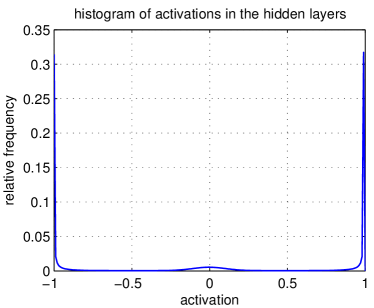
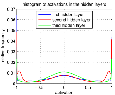
The activations in the last hidden layer are almost completely binary, see Figure 34a. This effect was also observed on an MLP with a single hidden layer, but is now even more pronounced. The activations in the other hidden layers are not binary: They frequently lie somewhere between $-1$ and $1$, see Figure 34b and resemble a typical distribution (Bengio and Glorot, 2010). The denoised output patches are therefore essentially constructed from binary codes weighting elements in a dictionary.

Figure 35: Information entropy of the units in the different hidden layers. All units in the last hidden layer have high entropy.

Entropy:

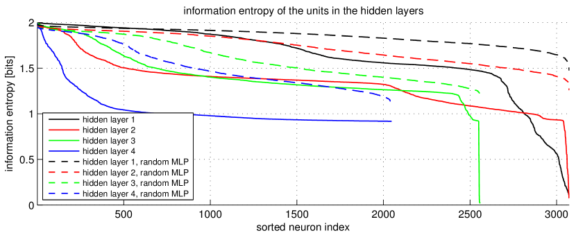
An MLP with a single hidden layer had some hidden units with entropy close to zero. Is this also the case for MLPs with more hidden layers? We evaluate the information entropy of the units in the various hidden layers, see Figure 35. We again used four bins of equal size. We also compare against a randomly initialized MLP. We observe that the entropy is lower for the trained MLP than for the randomly initialized MLP, which was also observed on an MLP with a single hidden layer. However, this time, all the units in the last hidden layer have high information entropy. In the remaining layers, some units have low information entropy.

feature detectors

feature detectors

Figure 36: Feature detectors of the units with the highest (top) and lowest (bottom) entropy.

feature generators

feature generators

Figure 37: Feature generators of the units with the highest (top) and lowest (bottom) entropy.

Figure 36 shows the feature detectors connected to the units with highest and lowest entropy, respectively. Figure 37 shows the feature generators with the highest and lowest entropy, respectively. The feature detectors with the highest entropy look different from the feature detectors with the lowest entropy. The latter all look similar: All are noisy and seem to loosely focus on a region in the center of the patch. The feature detectors with the highest entropy look more clearly defined. For the feature generators, no clear difference is observed. This is perhaps due to the fact that all output bases have high information entropy. The feature detectors with the lowest entropy almost always have the same activation value and are therefore probably also not very helpful in terms of denoising results.

image name	PSNR
Barbara	127.45dB
Boat	187.76dB
Cameraman	166.00dB
Couple	192.58dB
Fingerprint	198.12dB
Hill	192.05dB
House	195.68dB
Lena	192.19dB
Man	190.21dB
Montage	174.14dB
Peppers	189.49dB
Noise	161.28dB

Table 1: Ability of the dictionary to approximate images.

Figure 38: Spectrum of the output bases.

Approximation ability:

We have seen that the MLP does not perform as well as other methods on the image “Barbara”. We now ask the question: Is the dictionary formed by the last layer of the MLP the reason why some images cannot be denoised well? In other words, is it possible to approximate any image patch arbitrarily well using that dictionary, or are there images that are difficult to approximate? An additional constraint is that the code vector weighting the dictionary is not allowed to contain values below $-1$ or above $1$ due to the $\tanh$ layer.

To answer this question, we try to approximate images patch-wise using the dictionary formed by the last layer. In other words, we try to approximate each image patch $x$ of a clean image using our dictionary $D$, and proceed in a sliding-window manner. We average in the regions of overlapping patches. Formally, we solve the following problem:

$$\min||x-D\alpha||_{2}\quad\textrm{ s.t.}-1\preceq\alpha\preceq 1.$$ (1)

Table 1 lists the results obtained on the $11$ standard test images, as well as one image containing only white Gaussian noise with $\mu=127.5$ and $\sigma=25$ (row “Noise”). We see that all images (including the noise image) can be almost perfectly approximated, though the result on image Barbara is slightly worse than on other images. We therefore conclude that the dictionary in the last layer by itself cannot be the reason why some images are not denoised well. Any image can be well approximated using the dictionary and codes with values in range from -1 to 1.

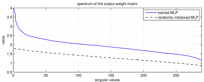
A related observation is that the weights in the last layer have no zero singular values, see Figure 38. This implies that the matrix has full rank and can therefore approximate any patch, when the lower- and upper-bound constraints are disregarded. We also observe that the spectrum is relatively flat, which was also the case for the MLP with a single hidden layer. This implies that the output bases are diverse.

image	KSVD (Aharon et al., 2006)	MLP	“MLP + OMP”
Barbara	29.49dB	29.52dB	28.23dB
Boat	29.24dB	29.95dB	28.93dB
Cameraman	28.64dB	29.60dB	28.32dB
Couple	28.87dB	29.75dB	28.66dB
Fingerprint	27.24dB	27.67dB	26.88dB
Hill	29.20dB	29.84dB	28.95dB
House	32.08dB	32.52dB	30.12dB
Lena	31.30dB	32.28dB	30.65dB
Man	29.08dB	29.85dB	28.95dB
Montage	30.91dB	31.97dB	30.21dB
Peppers	29.69dB	30.27dB	29.08dB

Table 2: Using the MLP’s dictionary in combination with OMP.

Combining the dictionary with sparse coding:

Dictionary-based methods for image denoising such as KSVD typically denoise by approximating a noisy image patch using a sparse linear combination of the elements in the dictionary. More formally, one attempts to solve the following problem:

$$\min||\alpha||_{0}\quad\textrm{s.t. }||y-D\alpha||_{2}\leq\epsilon$$ (2)

where $y$ is a noisy image patch, $\epsilon$ is a pre-defined parameter and $||\cdot||_{0}$ refers to the $\ell_{0}$ pseudo-norm. Approximate solutions to this problem can be found using OMP (Pati et al., 1993). The denoised patch $\hat{x}$ is given by $\hat{x}=D\alpha$. Denoising is performed in a sliding-window manner and averaging is performed where patches overlap.

We ask the question: Can the dictionary learned by the MLP be used in combination with this sparse coding approach? We denoise the $11$ standard test images with AWG noise, $\sigma=25$ using the dictionary learned by the MLP and solve equation (2) approximately using OMP. We set $\epsilon$ similarly to KSVD (Aharon et al., 2006): $\epsilon=n((C\sigma)^{2})$, where n is the dimensionality of the patches ($289$) and $C$ is a hyper-parameter. We found the best value of $C$ to be $1.05$. We normalized all columns of $D$ to have unit norm. The results of this approach are summarized in Table 2. The PSNR of the noisy images is approximately $20.18$dB.

The denoising results of this approach are not very good. We therefore conclude that the dictionary’s ability to denoise is strongly dependent on the codes provided to it. The first three hidden layers of the MLP serve as a mechanism for creating good codes for the last layer.

(a) Input patterns maximizing the activation of neurons in the second hidden layer.

(b) Natural image patches maximizing the absolute activation of neurons in the second hidden layer.

(c) Input patterns maximizing the activation of neurons in the third hidden layer.

(d) Natural image patches maximizing the absolute activation of neurons in the third hidden layer.

(e) Input patterns maximizing the activation of neurons in the fourth hidden layer.

(f) Natural image patches maximizing the absolute activation of neurons in the fourth hidden layer.

Figure 39: What features does the MLP respond to?

Inputs maximizing the activation of neurons:

Which inputs cause the highest activation for each neuron? We answer this question using two approaches: (i) Activation maximization (Erhan et al., 2010b) and (ii) evaluating the activation values for a large number of (non-noisy) image patches.

We perform activation maximization as described in section 31. We also run the MLP on a large number of noise-free natural image patches. For each neuron, we save the input maximizing its absolute activation. We used $6768$ natural images, each containing many thousand patches. Figure 39 shows the input patterns found through activation maximization as well as the input patches found by inspecting a larger number of natural image patches. We make a number of observations.

• Focus on the center part: The patterns found through activation maximization mostly focus on the center part of the patches. This intuitively makes sense: The most important part of the input patch is expected to be the area covered by the output patch. In addition, pixel correlations fall with distance, so pixels that are further away are expected to be less interesting. There are exceptions however: Some patches seem to focus particularly on the patch border.

• Gabor filters: Many input patterns resemble Gabor filters. This is true for all hidden layers, but particularly for hidden layers two and four. We also observed this phenomenon in the output layer weights, see Figure 33.

• Random looking patches: Many input patterns look as if the pixels were set randomly. This is particularly true in hidden layer three.

• Correlation to natural image patches: Some input patterns found through activation maximization correlate well with patches found through exhaustive search through a set of natural image patches. For example the patches $6$ and $7$ from the right in the upper row of hidden layer four. In many cases however, it is not clear that the two procedures find correlating patches. The fourth hidden layer patches seem to indicate that many neurons respond to features with a highly specific location and orientation.

4.4 Comparing the importance of the feature detectors

Some of the feature detectors look random or noisy, see Figure 33. Are all the feature detectors useful or are the noisy looking filters less useful? We answer this question by observing the behavior of the MLP when a set of feature detectors is removed (in other words, when only a subset of feature detectors is used). We evaluate the average performance of the network on the $11$ standard test images. We remove a feature detectors by replacing its weights with the average value of the feature detector.

feature detectors

feature detectors

Figure 40: Most (top) and least (bottom) important feature detectors (using 1500 feature detectors).

We use an iterative procedure during which $1500$ feature detectors are chosen for each iteration. The mean PSNR obtained is assigned to the feature detectors used during that iteration. We average over iterations. The feature detectors yielding the best results (on average) are shown in the top row of Figure 40 and the feature detectors yielding the worst results are shown in the bottom row.

It seems that the feature detectors yielding good results on average are more easily interpretable than the ones yielding worse results. The feature detectors yielding good results seem to focus on large-scale features, whereas the filters yielding worse results look more noisy.

4.5 Effect of the type and strength of the noise on the feature detectors and feature generators

All observations we have made on the feature detectors and feature generators of the MLPs were made on MLPs trained to remove AWG noise with $\sigma=25$. We will now make a number of observations for different types and strengths of noise.

feature detectors

feature generators

Figure 41: Random selection of weights in the input layer (top) and output layer (bottom) for $\sigma=10$

feature detectors

feature generators

Figure 42: Random selection of weights in the input layer (top) and output layer (bottom) for $\sigma=75$

How does the strength of the noise affect the learned weights? Figure 41 and Figure 42 show the feature detectors and feature generators for $\sigma=10$ and $\sigma=75$, respectively. The feature generators look similar for the two noise levels. However, the feature detectors look different: For $\sigma=10$, the feature detectors almost always focus on the area covered by the output patch, whereas for $\sigma=75$, the feature detectors also consider pixels that are further away. This is in agreement with Levin and Nadler (2011): When the noise is stronger, larger input patches are necessary to achieve good results. We already provided a similar explanation in Section 2.6. This also implies that it is unnecessary to use large input patches when the noise is weak and explains why we achieved better results with smaller patches for $\sigma=10$, see Figure 10.

feature detectors

feature generators

Figure 43: Random selection of weights in the input layer (top) and output layer (bottom) for stripe noise

feature detectors

feature generators

Figure 44: Random selection of weights in the input layer (top) and output layer (bottom) for salt and pepper noise

feature detectors

feature generators

Figure 45: Random selection of weights in the input layer (top) and output layer (bottom) for JPEG noise

How does the type of the noise affect the learned weights?

Figures 43, 44 and 45 show the feature detectors and feature generators learned with stripe noise, salt-and-pepper noise and JPEG artifacts, respectively. All patches in these figures are of size $17\times 17$. The input weights are strongly affected by the type of the noise: For horizontal stripe noise, the feature detectors often have horizontal features that also look like stripes. For salt-and-pepper noise, the feature detectors are often filters focussing on long edges. For JPEG artifacts, the feature detectors are close in appearance to the output weights. The feature generators are also somewhat affected by the type of the noise. This is especially visible for stripe noise, where the feature generators seem to sometimes also contain stripes. It was also observed by Vincent et al. (2010) that the type of the noise has a strong effect of the learned weights in denoising autoencoders.

output features

Figure 46: Block matching output weights

4.6 Block-matching filters

Figure 46 shows the feature generators learned by the MLP with block-matching, using $k=14$ and patches of size $13\times 13$. The feature generators look similar to those learned by MLPs without block-matching.

input features

Figure 47: Block matching input weights

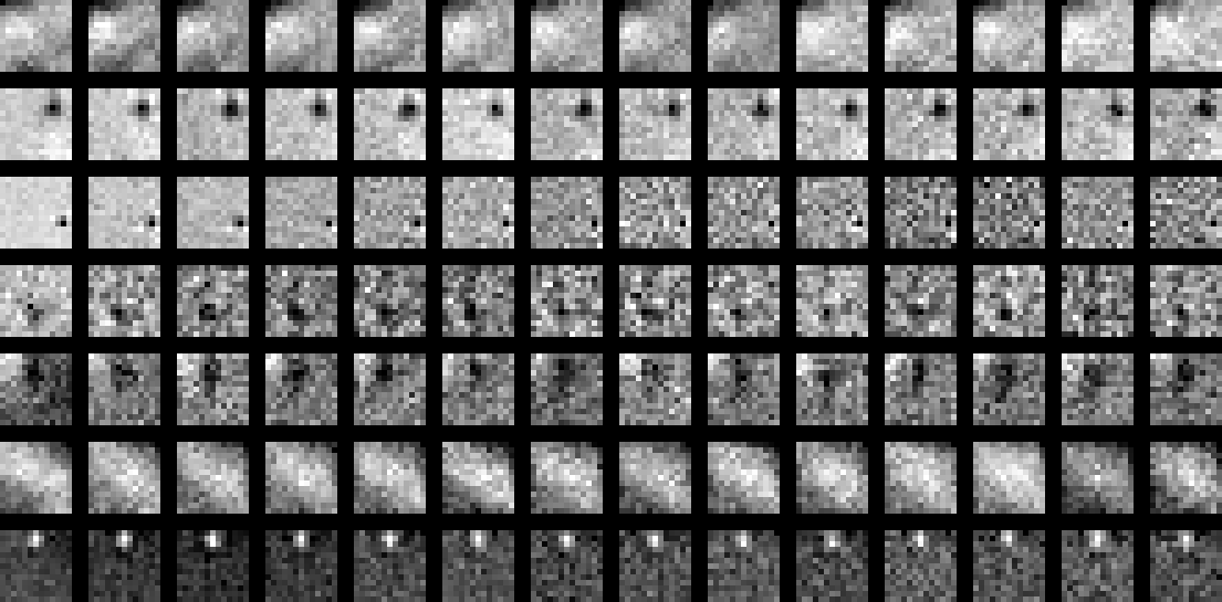
Figure 47 shows a selection of feature detectors learned by the MLP with block-matching. The left-most patch shows the filter applied to the reference patch, and the horizontally adjacent patches show the filters applied to the corresponding neighbor patches. The horizontally adjacent patches all connect to the same hidden neuron. We see that the filters applied to the neighbor patches are usually similar to the filters applied to the reference patch. This observation should not be surprising: The updates of the weights connecting the input patches to a hidden neuron are defined by (i) the gradient at the hidden neuron and (ii) the value of the input pixels. Hence, if the value of the input pixels are similar (this is ensured by the block-matching procedure), the weight updates are also similar.

5 Discussion and Conclusion

In Burger et al. (2012), we have shown that it is possible to achieve state-of-the-art image denoising results using MLPs. In this paper, we have shown how this is possible. In the first part of this paper, we have discussed which trade-offs are important during the training procedure. In the second part of this paper, we have shown that it is possible to gain insight about the inner working of the trained MLPs by analysing the activation patterns on the hidden units.

How to train MLPs:

We have trained MLPs with varying architectures on datasets of different sizes. We have also varied the sizes of the input as well as of the output patches. The observations made on these experiments allow us to make a number of conclusions regarding image denoising with MLPs: (i) More training data is always good, (ii) more hidden units per hidden layer is always good, (iii) there is an ideal number of hidden layers for a given problem and a given number of hidden units per hidden layer. Going above the ideal number of hidden layers can lead to catastrophic degradations in performance, (iv) increasing the output size requires higher-capacity architectures, and finally (v) fine-tuning with a lower learning rate can lead to important gains in performance.

Other image processing problems such as super-resolution, deconvolution and demosaicking might also be addressed using MLPs, in which case we expect the guidelines described in this paper to be useful as well. Other problems unrelated to images might also benefit from these guidelines. Indeed, we expect that many difficult problems with high dimensional inputs and outputs could benefit from these insights.

Understanding denoising MLPs:

The denoising procedure of MLPs with a single hidden layer can be briefly summarized as follows. Each hidden unit detects a feature in the noisy input and copies it to the output patch. Denoising is achieved through saturation of the $\tanh$-layer. The use of activation maximization (Erhan et al., 2010b) and observing outputs obtained by activating a single hidden unit in an MLP allowed us to make observations concerning the internal workings of MLPs with several hidden layers. We have seen that MLPs with several hidden layers seem to work according to the same principle as MLPs with a single hidden layer: The features required to maximize the activation of a hidden unit are often remarkably similar to the output caused by the same hidden unit. This observation is true for each hidden layer.

Denoising with MLPs requires that the $\tanh$-layer saturates, which naturally gives rise to binary representations. This is different from RBMs, which force their hidden representations to be binary. The fact that the representations are binary lends support to the regularization interpretation of denoising autoencoders proposed by Erhan et al. (2010a). We also note that binary representations are unusual for MLPs: Other problems do not give rise to binary representations (Bengio and Glorot, 2010).

As an alternative to binary representations, we consider sparse representations. Sparse representation in higher dimensional spaces have the well-known benefit of being able to more easily rely on linear operations for a variety of tasks, see for example Mairal et al. (2010). Sparsity has been proposed as a form of regularization to train deep belief networks, see Ranzato et al. (2007). Successful architectures for object recognition (Jarrett et al., 2009) also make use of sparse representations, in this case using a procedure called predictive sparse coding proposed by Kavukcuoglu et al. (2008). In all cases, achieving sparse representations requires sparsity inducing terms in the optimization criteria, which makes the optimization procedure more complex. We argue that binary representations have similar benefits to sparse representations, but that obtaining binary representations is easier than obtaining sparse representations, using a denoising criterion.

A further similarity between MLPs trained to denoise images and RBMs and denoising autoencoders is the similarity of the features (such as Gabor filters) learned by all three architectures. Unrelated approaches such KSVD (Aharon et al., 2006) learn similar features.

References

- Aharon et al. (2006) M. Aharon, M. Elad, and A. Bruckstein. K-svd: An algorithm for designing overcomplete dictionaries for sparse representation. IEEE Transactions on Signal Processing (TIP), 54(11):4311–4322, 2006.
- Bengio et al. (2007) Y. Bengio, P. Lamblin, D. Popovici, and H. Larochelle. Greedy layer-wise training of deep networks. Advances in neural information processing systems, 19:153, 2007.
- Bengio and Glorot (2010) Yoshua Bengio and Xavier Glorot. Understanding the difficulty of training deep feedforward neural networks. In Proceedings of AISTATS, volume 9, pages 249–256, 2010.
- Burger et al. (2012) H.C. Burger, C.J. Schuler, and S. Harmeling. Image denoising with multi-layer perceptrons, part 1: comparison with existing algorithms and with bounds. Submitted to the Journal of Machine Learning Research (JMLR), 2012.
- Chatterjee and Milanfar (2010) P. Chatterjee and P. Milanfar. Is denoising dead? IEEE Transactions on Image Processing (TIP), 19(4):895–911, 2010.
- Dabov et al. (2007) K. Dabov, A. Foi, V. Katkovnik, and K. Egiazarian. Image denoising by sparse 3-D transform-domain collaborative filtering. IEEE Transactions on Image Processing (TIP), 16(8):2080–2095, 2007.
- Erhan et al. (2010a) D. Erhan, Y. Bengio, A. Courville, P.A. Manzagol, P. Vincent, and S. Bengio. Why does unsupervised pre-training help deep learning? The Journal of Machine Learning Research (JMLR), 11:625–660, 2010a.
- Erhan et al. (2010b) D. Erhan, A. Courville, and Y. Bengio. Understanding representations learned in deep architectures. Technical report, Technical Report 1355, Université de Montréal/DIRO.(Cited on page 119.), 2010b.
- Hinton (2010) G. Hinton. A practical guide to training restricted boltzmann machines. Momentum, 9:1, 2010.
- Hinton (2002) G.E. Hinton. Training products of experts by minimizing contrastive divergence. Neural computation, 14(8):1771–1800, 2002.
- Hinton and Salakhutdinov (2006) G.E. Hinton and R.R. Salakhutdinov. Reducing the dimensionality of data with neural networks. Science, 313(5786):504–507, 2006.
- Hinton et al. (2006) G.E. Hinton, S. Osindero, and Y.W. Teh. A fast learning algorithm for deep belief nets. Neural Computation, 18(7):1527–1554, 2006.
- Jarrett et al. (2009) Kevin Jarrett, Koray Kavukcuoglu, Marc’Aurelio Ranzato, and Yann LeCun. What is the best multi-stage architecture for object recognition? In International Conference on Computer Vision (ICCV). IEEE, 2009.
- Kavukcuoglu et al. (2008) Koray Kavukcuoglu, Marc’Aurelio Ranzato, and Yann LeCun. Fast inference in sparse coding algorithms with applications to object recognition. Technical Report CBLL-TR-2008-12-01, Computational and Biological Learning Lab, Courant Institute, NYU, 2008.
- LeCun et al. (1998a) Y. LeCun, L. Bottou, Y. Bengio, and Haffner P. Gradient-based learning applied to document recognition. Proceedings of IEEE, 86(11):2278–2324, 1998a. URL http://leon.bottou.org/papers/lecun-98h.
- LeCun et al. (1998b) Y. LeCun, L. Bottou, G. Orr, and K. Müller. Efficient backprop. In Neural Networks, Tricks of the Trade, Lecture Notes in Computer Science LNCS 1524. Springer Verlag, 1998b. URL http://leon.bottou.org/papers/lecun-98x.
- Lee et al. (2009) H. Lee, R. Grosse, R. Ranganath, and A.Y. Ng. Convolutional deep belief networks for scalable unsupervised learning of hierarchical representations. In Proceedings of the 26th Annual International Conference on Machine Learning (ICML), pages 609–616. ACM, 2009.
- Levin and Nadler (2011) A. Levin and B. Nadler. Natural Image Denoising: Optimality and Inherent Bounds. In IEEE Conference on Computer Vision and Pattern Recognition (CVPR), 2011.
- Levin et al. (2012) A. Levin, B. Nadler, F. Durand, and W.T. Freeman. Patch complexity, finite pixel correlations and optimal denoising. In European Conference on Computer Vision (ECCV), 2012.
- Mairal et al. (2010) J. Mairal, F. Bach, J. Ponce, and G. Sapiro. Online learning for matrix factorization and sparse coding. The Journal of Machine Learning Research (JMLR), 11:19–60, 2010.
- Pati et al. (1993) Y.C. Pati, R. Rezaiifar, and PS Krishnaprasad. Orthogonal matching pursuit: Recursive function approximation with applications to wavelet decomposition. In Signals, Systems and Computers, 1993. 1993 Conference Record of The Twenty-Seventh Asilomar Conference on, pages 40–44. IEEE, 1993.
- Portilla et al. (2003) J. Portilla, V. Strela, M.J. Wainwright, and E.P. Simoncelli. Image denoising using scale mixtures of Gaussians in the wavelet domain. IEEE Transactions on Image Processing (TIP), 12(11):1338–1351, 2003.
- Ranzato et al. (2007) Marc’Aurelio Ranzato, Y. Boureau, and Y. LeCun. Sparse feature learning for deep belief networks. Advances in neural information processing systems, 20:1185–1192, 2007.
- Rossi (1978) J.P. Rossi. Digital techniques for reducing television noise. SMPTE Journal, 87(3):134–140, 1978.
- Vincent et al. (2010) P. Vincent, H. Larochelle, I. Lajoie, Y. Bengio, and P.A. Manzagol. Stacked denoising autoencoders: Learning useful representations in a deep network with a local denoising criterion. The Journal of Machine Learning Research (JMLR), 11:3371–3408, 2010.