Constrained energy minimization and orbital stability for the NLS equation on a star graph

Abstract.

We consider a nonlinear Schrödinger equation with focusing nonlinearity of power type on a star graph ${\mathcal{G}}$, written as $i\partial_{t}\Psi(t)=H\Psi(t)-|\Psi(t)|^{2\mu}\Psi(t)$ , where $H$ is the selfadjoint operator which defines the linear dynamics on the graph with an attractive $\delta$ interaction, with strength $\alpha<0$, at the vertex. The mass and energy functionals are conserved by the flow. We show that for $0<\mu<2$ the energy at fixed mass is bounded from below and that for every mass $m$ below a critical mass $m^{*}$ it attains its minimum value at a certain $\hat{\Psi}_{m}\in H^{1}(\mathcal{G})$, while for $m>m^{*}$ there is no minimum. Moreover, the set of minimizers has the structure ${\mathcal{M}}=\{e^{i\theta}\hat{\Psi}_{m}\ ,\theta\in\mathbb{R}\}$. Correspondingly, for every $m<m^{*}$ there exists a unique $\omega=\omega(m)$ such that the standing wave $\hat{\Psi}_{\omega}e^{i\omega t}$ is orbitally stable. To prove the above results we adapt the concentration-compactness method to the case of a star graph. This is non trivial due to the lack of translational symmetry of the set supporting the dynamics, i.e. the graph. This affects in an essential way the proof and the statement of concentration-compactness lemma and its application to minimization of constrained energy. The existence of a mass threshold comes from the instability of the system in the free (or Kirchhoff’s) case, that in our setting corresponds to $\alpha=0$.

1. Introduction

In the present paper we study the minimization of a constrained energy functional defined on a star graph and its application to existence and stability of standing waves for nonlinear Schrödinger propagation with an attractive interaction at the vertex of the graph.

We recall that in our setting a star graph $\mathcal{G}$ is the union of $N$ half-lines (edges) connected at a single vertex; the Hilbert space on $\mathcal{G}$ is $L^{2}(\mathcal{G})=\bigoplus_{j=1}^{N}L^{2}(\mathbb{R}^{+})$. We denote the elements of $L^{2}(\mathcal{G})$ by capital Greek letters, while functions in $L^{2}(\mathbb{R}^{+})$ are denoted by lowercase Greek letters. The elements of $L^{2}(\mathcal{G})$ can be represented as column vectors of functions in $L^{2}(\mathbb{R}^{+})$, i.e.

$$\Psi=\begin{pmatrix}\psi_{1}\\ \vdots\\ \psi_{N}\end{pmatrix}.$$

We shall also use the notation $\psi_{i}(x)\equiv(\Psi)_{i}(x)\equiv\Psi(x,i)$. Notice that the set $\mathcal{G}$ has not to be thought of as embedded in $\mathbb{R}^{n}$, so it has no geometric properties such as angles between edges. When an element of $L^{2}(\mathcal{G})$ evolves in time, to highlight the dependence on the time parameter $t$, we use both the notation $\Psi(t)$ and the one with subscript $t$, for instance $\Psi_{t}$.

In order to define a selfadjoint operator $H_{\mathcal{G}}$ on $\mathcal{G}$ one has to introduce operators acting on the edges and to prescribe a suitable boundary condition at the vertex that defines ${\mathcal{D}}(H_{\mathcal{G}})$, see, e.g., [KS99]. A metric graph equipped with a dynamics associated to a Hamiltonian of the form of $H_{\mathcal{G}}$ is called quantum graph. On a quantum graph one can consider the dynamics defined by the abstract Schrödinger equation given by

$$i\partial_{t}\Psi(t)\ =\ H_{\mathcal{G}}\Psi(t)\ ,\ \ \Psi\in{\mathcal{D}}(H_{\mathcal{G}}).$$

From a formal point of view the previous equation is equivalent to a system of $N$ Schrödinger equations on the half-line coupled through the boundary condition at the vertex.

Of course the graph could be more general than a star graph, with several (possibly infinite) vertices, bounded edges connecting them (sometimes called bonds as suggested from chemistry applications) and unbounded edges, as in the present case of star graphs or in the interesting case of trees with the last generation of edges of infinite length.

The analysis of linear dispersive equations on graphs, in particular of the Schrödinger equation, is a quite developed subject with a wide range of applications from chemistry and nanotechnology to quantum chaos. We refer to [BCFK06, BEH08, EKK⁺08, Kuc04, Kuc05] for further information and bibliography.

On the contrary, the study of nonlinear equations on networks is in general a subject at its beginnings. Some results concerning nonlinear PDE’s on graphs are given in [CM07] for reaction-diffusion equations (see references therein) and in the recent paper [CMS12] for the Hamilton-Jacobi equation (with reference to previous work on fully nonlinear equations). As regards semilinear dispersive equations we mention the preliminary work on NLS in the cubic case in [CH10], and for a different nonlinear dispersive equation related to long water waves, the BBM equation, the results given in [BC08].

One way to define a nonlinear Schrödinger dynamics (NLS) on a graph, mimicking the linear case, consists in prescribing the NLS on every single edge and requiring its strong solution to satisfy a boundary condition at the vertex at every time, i.e. imposing the solution to remain at any time in the domain of the generator of the linear dynamics. In strong formulation, one obtains the equation

$$i\partial_{t}\Psi(t)\ =\ H_{\mathcal{G}}\Psi(t)+G(\Psi(t)),\ \ \Psi(t)\in{\mathcal{D}}(H_{\mathcal{G}})\ ,$$

where the nonlinearity $G=(G_{1},\cdots,G_{N}):\mathbb{C}^{N}\rightarrow\mathbb{C}^{N}$ acts “componentwise” as $G_{i}(\zeta)=g(|\zeta_{i}|)\zeta_{i}$ for a suitable $g:\mathbb{R}^{+}\rightarrow\mathbb{R}$ and $\zeta=(\zeta_{1},\cdots,\zeta_{N})\in\mathbb{C}^{N}$. More general nonlinearities of nonlocal type which couple different edges are possible at a mathematical level, but they seem to be less interesting from the physical point of view.

The analysis of nonlinear propagation on graphs, as in the more standard case of $\mathbb{R}^{n}$, proceeds along two main lines of development: the study of dispersive and scattering behavior (see [ACFN11] and reference therein; see also [BI11] for relevant work about dispersion on trees) and the study of bound states (see [ACFN12a, ACFN12b, ACFN12c] and reference therein). In this paper we concentrate on this last item. We shall focus on a concrete model and not on a general class specifying the nonlinearity and the interaction at the vertex of the star graph, which means to give the function $g$ and the selfadjoint operator $H_{\mathcal{G}}$. Concerning the first, we treat a power nonlinearity of focusing type, i.e. $g(z)=-|z|^{2\mu},\ \mu>0\ .$ This choice has two main reasons. It corresponds to the most usual models considered in the physical applications, and moreover it allows to have some explicit and quantitative estimates needed in the proofs of our results which could be difficult to obtain for general nonlinearities.

To motivate the choice of the linear part $H_{\mathcal{G}}$ we begin to remark that the meaning of the boundary condition is to describe suitable local interactions occurring between different components of the wavefunction on different edges. For example, one could be interested in describing the effect of the presence of a localized potential well at the vertex. This corresponds in the linear case to a confining potential admitting one or more bound states. In the case of a NLS on the line or more generally on $\mathbb{R}^{n}$, the presence of a negative potential entails the existence of trapped solitons sitting around the minima of the potential well. These trapped solitons, of the form $\Psi(t)=\Psi_{\omega}e^{i\omega t}$ where $\omega$ belongs to some subset of the real line, are usually called standing waves, and are studied for example in [GS07, GSS87a, GSS87b, GNT04, Wei86], to which we refer for information and further references concerning their existence, variational properties, orbital and asymptotic stability. Here we address the analogous problem in the context of star graphs. To fix the model we consider the so called $\delta$ vertex, which is one of the most common in the applications to quantum graphs.

We introduce preliminarily some notations and define several functional spaces on the graph.

The norm of $L^{2}$-functions on $\mathcal{G}$ is naturally defined by

$$\|\Psi\|^{2}_{L^{2}(\mathcal{G})}:=\sum_{j=1}^{N}\|\psi_{j}\|^{2}_{L^{2}(\mathbb{R}^{+})}.$$

From now on for the $L^{2}$-norm on the graph we drop the subscript and simply write $\|\cdot\|$. Accordingly, we denote by $(\cdot,\cdot)$ the scalar product in $L^{2}(\mathcal{G})$.

Analogously, given $1\leq r\leq\infty$, we define the space $L^{r}(\mathcal{G})$ as the set of functions on the graph whose components are elements of the space $L^{r}(\mathbb{R}^{+})$, and the norm is correspondingly defined by

$$\big{\|}\Psi\big{\|}_{r}^{r}=\sum_{j=1}^{N}\|\psi_{j}\|_{L^{r}(\mathbb{R}^{+})}^{r},\ 1\leq r<\infty,\qquad\big{\|}\Psi\big{\|}_{\infty}=\max_{1\leq j\leq N}\|\psi_{j}\|_{L^{\infty}(\mathbb{R}^{+})}.$$

Besides, we need to introduce the spaces

$$H^{1}(\mathcal{G})\equiv\bigoplus_{j=1}^{N}H^{1}(\mathbb{R}^{+})\qquad H^{2}(\mathcal{G})\equiv\bigoplus_{j=1}^{N}H^{2}(\mathbb{R}^{+}),$$

equipped with the norms

$$\|\Psi\|_{H^{1}}^{2}\ =\ \sum_{i=1}^{N}\|\psi_{i}\|_{H^{1}(\mathbb{R}^{+})}^{2},\qquad\|\Psi\|_{H^{2}}^{2}\ =\ \sum_{i=1}^{N}\|\psi_{i}\|_{H^{2}(\mathbb{R}^{+})}^{2}.$$

Notice that there is a slight abuse in the denominations ${H^{i}}(\mathcal{G})$ for the above spaces, because their elements have no Sobolev regularity at the vertex.

However they have boundary values on each edge, and we denote without comment the notation $\psi(0^{+})=\psi(0)$ for every $\psi\in H^{i}(\mathbb{R}^{+})\ ,i=1,2\ .$ In the following, whenever a functional norm refers to a function defined on the graph, we omit the symbol $\mathcal{G}$.

We denote by $H$ the Hamiltonian with $\delta$ coupling in the vertex of strength $\alpha$, where $\alpha\in\mathbb{R}$. It is defined as the operator in $L^{2}$ with domain

$${\mathcal{D}}(H):=\left\{\Psi\in H^{2}\text{ s.t. }\psi_{1}(0)=\ldots=\psi_{N}(0),\,\sum_{k=1}^{N}\psi_{k}^{\prime}(0)=\alpha\psi_{1}(0)\right\}.$$

and action

$$H\Psi=\begin{pmatrix}-\psi_{1}^{\prime\prime}\\ \vdots\\ -\psi_{N}^{\prime\prime}\end{pmatrix}.$$

In the present paper we will consider only the case of attractive $\delta$ interaction, i.e. $\alpha<0$. Sometimes to make explicit the fact that $\alpha<0$ we set $\alpha=-|\alpha|$.

It is well known that the operator $H$ is a selfadjoint operator on $L^{2}$, see, e.g., [KS99]. Moreover for $\alpha<0$ the operator $H$ admits a single bound state associated to the eigenvalue $-{\alpha^{2}}/{N^{2}}$, in this sense the $\delta$ interaction can be considered as a singular potential well placed at the vertex.

The definition of $H$ and its scope is analogous to the case of the attractive $\delta$ potential on the line, widely used in theoretical and applied physics to describe situations of strongly localized interactions such as trapping defects in a elsewhere homogeneous medium. This is justified in view of the fact that the operator $H$ is a norm resolvent limit of regular Schrödinger operators on the star graph with regular potentials $V_{\epsilon}$ scaling as a $\delta$-like sequence picked at the vertex (see, e.g., [Exn96])

This ends the construction and mathematical justification of the model, which is finally described by the equation

(1.1) $$i\partial_{t}\Psi(t)\ =\ H\Psi(t)-|\Psi(t)|^{2\mu}\Psi(t),\ \ \Psi\in{\mathcal{D}}(H).$$

From the point of view of physical applications the problem described by the above equation is interesting in relation to the so called Y-junctions or beam splitters in the study of Bose-Einstein condensates (see [TOD08]). Other problems related to nonlinear Schrödinger propagation on graphs are treated in [GSD11, MMK07, SMS⁺10], and more generally there is a growing interest in nonlinear propagation on networks, both in nonlinear optics and in Bose condensates, which are the main fields of application of the NLS.

From the mathematical point of view, several results on the nonlinear model (1.1) were given in a series of papers ([ACFN11, ACFN12a, ACFN12b, ACFN12c]). In particular we refer to the work [ACFN12c] which is a companion to the present one, where a variational study of the standing waves and their orbital stability is performed according to the Grillakis-Shatah-Strauss method ([GSS87a, GSS87b]). While in [ACFN12c] the interesting functional is the action, minimized on the Nehari manifold, here we minimize the energy at constant norm following the Cazenave-Lions approach to orbital stability, see [CL82] (see also [Caz03, Caz06]). As it is shown elsewhere (see [ACFN12c]) the dynamical system (1.1) has two conserved quantities, the mass

(1.2) $$M[\Psi]=\|\Psi\|^{2}$$

and the energy $E$, which in our case reads

(1.3) $$E[\Psi]=\frac{1}{2}\|\Psi^{\prime}\|^{2}-\frac{1}{2\mu+2}\|\Psi\|_{2\mu+2}^{2\mu+2}+\frac{\alpha}{2}|\psi_{1}(0)|^{2}.$$

The energy domain $\mathcal{E}$ coincides with the domain of the quadratic form associated to the linear generator $H$, consisting of $H^{1}$ functions on every edge with continuity at the vertex

$${\mathcal{E}}:=\left\{\Psi\in H^{1}\text{ s.t.}\ \psi_{1}(0)=\cdots=\psi_{N}(0)\right\}.$$

On this domain we show that the energy $E[\Psi]$ is bounded from below if the mass $\|\Psi\|^{2}$ is fixed.

We are then interested in characterizing the ground state of this system. By ground state we mean the minimizer $\hat{\Psi}$ (if existing) of the energy $E$ in $\mathcal{E}$ constrained to the manifold of the states with fixed mass $m$.

As noticed before, the classical method which allows to treat this kind of problems is the concentration-compactness principle of P.-L. Lions with its application to the NLS given in [CL82]). A study of ground states for NLS on the line with several kind of defects (including the $\delta$ potential) making use of a concentration compactness is given in [ANV12]. Nevertheless, the present situation needs some non trivial modifications of the method, due to the fact that a graph, and in particular a star graph, does not enjoy translational symmetry, nor other kinds of symmetry needed to apply concentration-compactness in its direct form (see [TF07] for a very general presentation and applications of the method). We will adapt the concentration-compactness lemma (as given in [Caz03, Ch. 1 and 8] and also in [Caz06], which we will take as reference formulation in the course of our treatment) modifying the statement and the proof to draw our main conclusions on the minimum problem we are interested in. For more extended discussion on the novelties of this approach, we refer to Section 3. Using the concentration-compactness lemma we prove the following result which states the existence of the solution of the constrained minimization problem for small enough mass.

Theorem 1.

Let $m^{\ast}$ be defined by

(1.4) $$m^{\ast}=2\frac{(\mu+1)^{1/\mu}}{\mu}\,\left(\frac{|\alpha|}{N}\right)^{\frac{2-\mu}{\mu}}\int_{0}^{1}(1-t^{2})^{\frac{1}{\mu}-1}\,dt.$$

Let $\alpha<0$ and assume $m\leq m^{\ast}$ if $0<\mu<2$ and $m<\min\{{m^{\ast},\frac{\pi\sqrt{3}N}{4}}\}$ if $\mu=2$ and set

$$-\nu=\inf\{E[\Psi]\textrm{ s.t. }\Psi\in\mathcal{E}\,,\;M[\Psi]=m\}\,.$$

Then $0<\nu<\infty$ and there exists $\hat{\Psi}$ such that $M[\hat{\Psi}]=m$ and $E[\hat{\Psi}]=-\nu$.

By the phase invariance of equation (1.1) one has that the family of ground states is given by

$${\mathcal{M}}=\{e^{i\theta}\hat{\Psi}\ ,\theta\in\mathbb{R}\}\ .$$

The explicit expression of $\hat{\Psi}$ can be given. To this end, let us recall several results from [ACFN12b] and [ACFN12c]. For any $\omega>0$, we label the soliton profile on the real line as

(1.5) $$\phi_{\omega}(x)=[(\mu+1)\omega]^{\frac{1}{2\mu}}\operatorname{sech}^{\frac{1}{\mu}}(\mu\sqrt{\omega}x).$$

For any $\alpha<0$, $j=0,...,\left[\frac{N-1}{2}\right]$ ($[x]$ denoting the integer part of $x$) and $\omega>\frac{\alpha^{2}}{(N-2j)^{2}}$ we define $\Psi_{\omega,j}$ as

(1.6) $$\left(\Psi_{\omega,j}\right)(x,i)=\begin{cases}\phi_{\omega}(x-a_{j})&i=1,\ldots,j\\ \phi_{\omega}(x+a_{j})&i=j+1,\ldots,N\end{cases}$$

with

(1.7) $$a_{j}=\frac{1}{\mu\sqrt{\omega}}\operatorname{arctanh}\left(\frac{|\alpha|}{(N-2j)\sqrt{\omega}}\right).$$

The functions $\Psi_{\omega,j}\in\mathcal{D}(H)$ and are solutions of the stationary equation

(1.8) $$H\Psi_{\omega}-|\Psi_{\omega}|^{2\mu}\Psi_{\omega}=-\omega\Psi_{\omega}.$$

We say that $\Psi_{\omega,j}$ has a “bump” (resp. a “tail”) on the edge $i$ if $\left(\Psi_{\omega,j}\right)(x,i)$ is of the form $\phi_{\omega}(x-a_{j})$ (resp. $\phi_{\omega}(x+a_{j})$). The index $j$ in $\Psi_{\omega,j}$ denotes the number of bumps of the state $\Psi_{\omega,j}$. For this reason, we refer to the stationary state $\Psi_{\omega,0}$ as the “$N$-tail state”. We remark that the $N$-tail state is the only symmetric (i.e. invariant under permutation of the edges) solution of equation (1.8). For $j\geq 1$ there are $\binom{N}{j}$ distinct solutions obtained by formulae (1.6) and (1.7) by positioning the bumps on the edges in all the possible ways. For instance, if $N=3$ then there are two stationary states, a three-tail state and a two-tail/one-bump state. They are shown in figure 1.

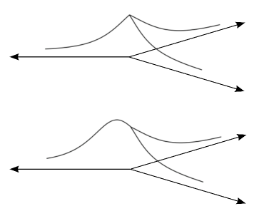
Figure 1. Stationary states for $N=3$, $\alpha<0$ .

Theorem 2.

Let $\alpha<0$ and assume $m\leq m^{\ast}$ if $0<\mu<2$ and $m<\min\{m^{\ast},\frac{\pi\sqrt{3}N}{4}\}$ if $\mu=2$; then the minimizer $\hat{\Psi}$ coincides with the $N$-tail state defined by $\Psi_{\omega_{0},0}$ where $\omega_{0}$ is chosen such that $M[\Psi_{\omega_{0},0}]=m$.

Since the minimizer $\hat{\Psi}$ is a stationary state, in order to prove Th. 2 it is sufficient to show that $\Psi_{\omega_{0},0}$ has minimum energy among the set of stationary states, which is finite. In facts in Section 5 we shall prove a more detailed statement; the energies of the stationary states, with frequencies $\omega_{j}$ such that $M[\Psi_{\omega_{j},j}]=m$, are increasing in $j$, i.e. they can be ordered in the number of the bumps, see Lem. 5.2. Notice that the bounds on thresholds in $m$ are different in the critical and subcritical case. More remarks on this are given in Section 5. Notice that as a consequence we have that the ground state of the system is the only stationary state which is symmetrical with respect to permutation of edges.

Finally, making use of the classical argument of Cazenave and Lions [CL82], from mass and energy conservation laws, convergence of the minimizing sequences and uniqueness of the ground state up to phase shift shown in Th. 1 and Th. 2, the orbital stability of the ground state follows. A detailed proof will not be given, being straightforward extension of the previous outline.

Corollary 1.

Let $\alpha<0$ and assume $m\leq m^{\ast}$ if $0<\mu<2$ and $m<\min\{m^{\ast},\frac{\pi\sqrt{3}N}{4}\}$ if $\mu=2$; then $\Psi_{\omega_{0},0}$ is orbitally stable.

The paper is organized as follows. In Section 2 we recall several known results which will be needed in the proof of Th. 1. In Section 3 we prove the concentration-compactness lemma for star graphs. Section 4 is devoted to the proof of Th. 1. In Section 5 we analyze the frequency and energy of stationary states on the manifold of constant mass and prove Th. 2.

2. Preliminaries

In this section we fix some notation and recall several results mostly taken from [ACFN12c]. We shall denote generic positive constants by $c$, in the proof the value of $c$ will not be specified and can change from line to line. The dual of $\mathcal{E}$ will be denoted by $\mathcal{E}^{\star}$. We shall denote the points of the star graph by $\underline{x}\equiv(x,j)$ with $x\in\mathbb{R}^{+}$ and $j\in\{1,\ldots,N\}$.

2.1. Well-posedness

We recall that equation (1.1) can be understood in the weak form given by

(2.1) $$\Psi(t)\ =\ e^{-iHt}\Psi_{0}-i\int_{0}^{t}e^{-iH(t-s)}|\Psi(s)|^{2\mu}\Psi(s)\,ds$$

with $\Psi_{0}\equiv\Psi(t=0)$.

As in the standard NLS on the line, mass and energy, Eqs. (1.2) and (1.3), are conserved by the flow, see Prop. 2.2 in [ACFN12c]. Moreover, if $0<\mu<2$, then the equation (2.1) is well posed in the energy domain and the solution is global, see Cor. 2.1 in [ACFN12c]. More precisely we have

Proposition 2.1 (Local well-posedness in $\mathcal{E}$).

Let $\mu>0$. For any $\Psi_{0}\in\mathcal{E}$, there exists $T>0$ such that the equation (2.1) has a unique solution $\Psi\in C^{0}([0,T),\mathcal{E})\cap C^{1}([0,T),\mathcal{E}^{\star})$. Moreover, Eq. (2.1) has a maximal solution $\Psi^{\rm{max}}$ defined on an interval of the form $[0,T^{\star})$, and the following “blow-up alternative” holds: either $T^{\star}=\infty$ or

$$\lim_{t\to T^{\star}}\|\Psi_{t}^{\rm{max}}\|_{\mathcal{E}}\ =\ +\infty,$$

where we denoted by $\Psi_{t}^{\rm{max}}$ the function $\Psi^{\rm{max}}$ evaluated at time $t$.

Proposition 2.2 (Conservation laws).

Let $\mu>0$. For any solution $\Psi\in C^{0}([0,T),\mathcal{E})\cap C^{1}([0,T),\mathcal{E}^{\star})$ to the problem (2.1), the following conservation laws hold at any time $t$:

$$M[\Psi_{t}]\ =M[\Psi_{0}],\qquad E[\Psi_{t}]\ =\ E[\Psi_{0}].$$

Corollary 2 (Global well posedness).

Let $0<\mu<2$. For any $\Psi_{0}\in\mathcal{E}$, the equation (2.1) has a unique solution $\Psi\in C^{0}([0,\infty),\mathcal{E})\cap C^{1}([0,\infty),\mathcal{E}^{\star})$.

2.2. Kirchhoff coupling

The vertex coupling associated to $\alpha=0$, is usually called free (on the line the interaction disappears) or Kirchhoff coupling and plays a distinguished role. For this reason we shall denote by $H^{0}$ the corresponding operator defined by

$${\mathcal{D}}(H^{0}):=\{\Psi\in H^{2}\text{ s.t. }\,\psi_{1}(0)=\ldots=\psi_{N}(0),\,\sum_{i=1}^{N}\psi_{i}^{\prime}(0)=0\}$$

$$H^{0}\Psi=\begin{pmatrix}-\psi_{1}^{\prime\prime}\\ \vdots\\ -\psi_{N}^{\prime\prime}\end{pmatrix}.$$

We also define the corresponding energy functional

(2.2) $$E^{0}[\Psi]=\frac{1}{2}\|\Psi^{\prime}\|-\frac{1}{2\mu+2}\|\Psi\|_{2\mu+2}^{2\mu+2}$$

with energy domain $\mathcal{D}(E^{0})=\mathcal{E}$.

2.3. Gagliardo-Nirenberg inequalities

We shall use a version of Gagliardo-Nirenberg inequalities on the star graph. The following proposition is a direct consequence of the Gagliardo-Nirenberg inequalities on the half-line see, e.g., [MPF91, I.31].

Proposition 2.3 (Gagliardo-Nirenberg Inequality).

Let $2\leq q\leq+\infty$, $1\leq p\leq q$ and set $a=\frac{\frac{1}{p}-\frac{1}{q}}{\frac{1}{2}+\frac{1}{p}}$, then for any $\Psi\in H^{1}$

$$\|\Psi\|_{q}\leq c\|\Psi^{\prime}\|^{a}\|\Psi\|_{p}^{1-a}\,.$$

2.4. Symmetric rearrangements

Here we recall the basic properties of symmetric rearrangements on a star graph introduced in [ACFN12c]. For a given function $\Phi:\mathcal{G}\to\mathbb{C}^{N}$ one introduces the rearranged function $\Phi^{*}:\mathcal{G}\to\mathbb{R}^{N}$. The function $\Phi^{*}$ is positive, symmetric, non increasing and is constructed in such a way that it is equimisurable w.r.t. $\Phi$, that is, the level sets of $|\Phi|$ and $\Phi^{*}$ have the same measure. This is sufficient to prove that all the $L^{p}(\mathcal{G})$ norms are conserved by the rearrangement. The comparison of the kinetic energy of $\Phi$ and $\Phi^{*}$ is more delicate. On the real line the Pólya-Szegő inequality shows that the kinetic energy does not increase. This is no longer true for a star graph where a constant $N/2$ appears, see Prop. 2.6 below.

Definition 2.4 (Symmetric rearrangement).

Given $\Psi:\mathcal{G}\to\mathbb{C}^{N}$, let $\lambda:\mathcal{G}\to\mathbb{R}$ be given by $\lambda(s)=|\{|\Psi|\geq s\}|$ (which is the measure of the set $\{\underline{x}\textrm{ s.t. }|\Psi(\underline{x})|\geq s\}$) and $g:\mathbb{R}^{+}\to\mathbb{R}^{+}$ be $g(t)=\sup\{s|\,\lambda(s)>Nt\}$. The symmetric rearrangement $\Psi^{\ast}$ of $\Psi$ is defined by $\Psi^{*}=(\psi^{*}_{1},...,\psi^{*}_{N})^{T}$ with

$$\psi^{*}_{1}(x)=...=\psi^{*}_{N}(x)=g(x).$$

The main properties of $\Psi^{\ast}$ are the following:

Proposition 2.5.

The symmetric rearrangement $\Psi^{\ast}$ is positive, symmetric and non increasing. Moreover, $\|\Psi^{\ast}\|_{p}=\|\Psi\|_{p}$.

Proposition 2.6 (Pólya-Szegő inequality for star graphs).

Assume that $\Psi\in H^{1}$. Then $\Psi^{\ast}\in H^{1}$ and

$$\|{\Psi^{\ast}}^{\prime}\|\leq\frac{N}{2}\|\Psi^{\prime}\|.$$

2.5. Mass and energy on the half-line and on the line

For later convenience we introduce also the unperturbed energy and mass functional for functions belonging to $H^{1}(\mathbb{R}^{+})$ and $H^{1}(\mathbb{R})$. For the half-line we denote the functionals by $M_{\mathbb{R}^{+}}$ and $E_{\mathbb{R}^{+}}$, respectively. They are defined by

$$M_{\mathbb{R}^{+}}[\psi]=\|\psi\|^{2}_{L^{2}(\mathbb{R}^{+})}$$

$$E_{\mathbb{R}^{+}}^{0}[\psi]=\frac{1}{2}\|\psi^{\prime}\|^{2}_{L^{2}(\mathbb{R}^{+})}-\frac{1}{2\mu+2}\|\psi\|^{2\mu+2}_{L^{2\mu+2}(\mathbb{R}^{+})}.$$

For the line we denote the mass end energy functionals by $M_{\mathbb{R}}$ and $E_{\mathbb{R}}$, respectively. They are defined by

$$M_{\mathbb{R}}[\psi]=\|\psi\|^{2}_{L^{2}(\mathbb{R})}$$

$$E_{\mathbb{R}}^{0}[\psi]=\frac{1}{2}\|\psi^{\prime}\|^{2}_{L^{2}(\mathbb{R})}-\frac{1}{2\mu+2}\|\psi\|^{2\mu+2}_{L^{2\mu+2}(\mathbb{R})}.$$

Using the definition (1.5) and a change of variable, one obtains the following formulas:

(2.3) $$\int_{0}^{\infty}|\phi_{\omega}(x+\xi)|^{2}dx\quad=\frac{(\mu+1)^{\frac{1}{\mu}}}{\mu}\omega^{\frac{1}{\mu}-\frac{1}{2}}\int^{1}_{\tanh(\xi\mu\sqrt{\omega})}(1-t^{2})^{\frac{1}{\mu}-1}dt$$

(2.4) $$\int_{0}^{\infty}|\phi_{\omega}(x+\xi)|^{2\mu+2}dx=\frac{(\mu+1)^{1+\frac{1}{\mu}}}{\mu}\omega^{\frac{1}{\mu}+\frac{1}{2}}\int^{1}_{\tanh(\xi\mu\sqrt{\omega})}(1-t^{2})^{\frac{1}{\mu}}dt.$$

The mass and energy functional evaluated on the soliton are given by

(2.5) $$M_{\mathbb{R}}[\phi_{\omega}]=2M_{\mathbb{R}^{+}}[\phi_{\omega}]=2\frac{(\mu+1)^{\frac{1}{\mu}}}{\mu}\omega^{\frac{1}{\mu}-\frac{1}{2}}\int_{0}^{1}(1-t^{2})^{\frac{1}{\mu}-1}dt,$$

(2.6) $$E^{0}_{\mathbb{R}}[\phi_{\omega}]=2E^{0}_{\mathbb{R}^{+}}[\phi_{\omega}]=-\frac{(\mu+1)^{\frac{1}{\mu}}}{\mu}\frac{2-\mu}{2+\mu}\omega^{\frac{1}{\mu}+\frac{1}{2}}\int_{0}^{1}(1-t^{2})^{\frac{1}{\mu}-1}dt,$$

where we used the identity

(2.7) $$\left(\frac{1}{2}+\frac{1}{\mu}\right)\int^{1}_{b}(1-t^{2})^{\frac{1}{\mu}}dt=-\frac{b}{2}(1-b^{2})^{\frac{1}{\mu}}+\frac{1}{\mu}\int^{1}_{b}(1-t^{2})^{\frac{1}{\mu}-1}dt.$$

It is well known that the function $\phi_{\omega}$ minimizes $E_{\mathbb{R}}$ at fixed mass. More precisely, choose $\overline{\omega}$ such that $M_{\mathbb{R}}[\phi_{\overline{\omega}}]=m$, then $\phi_{\overline{\omega}}$ is a minimizer of the problem

$$\inf_{\stackrel{{\scriptstyle\psi\in H^{1}(\mathbb{R})}}{{M_{\mathbb{R}}[\psi]=m}}}E_{\mathbb{R}}^{0}[\psi].$$

This also implies that $\phi_{\omega}$, with $\omega$ such that $M_{\mathbb{R}^{+}}[\phi_{\omega}]=m$, is the solution to the problem

$$\inf_{\stackrel{{\scriptstyle\psi\in H^{1}(\mathbb{R}^{+})}}{{M_{\mathbb{R}^{+}}[\psi]=m}}}E_{\mathbb{R}^{+}}[\psi].$$

To prove the last statement, assume that $f\in H^{1}(\mathbb{R}^{+})$ is such that $M_{\mathbb{R}^{+}}[f]=m$ and

$$E^{0}_{\mathbb{R}^{+}}[f]\leq E_{\mathbb{R}^{+}}[\phi_{\omega}]$$

where $\omega$ is chosen to satisfy $M_{\mathbb{R}^{+}}[\phi_{\omega}]=m$. Then, denoted by $\tilde{f}$ the even extension of $f$, one would obtain

$$E^{0}_{\mathbb{R}}[\tilde{f}]\leq E^{0}_{\mathbb{R}}[\phi_{\omega}]$$

where $M_{\mathbb{R}}[\tilde{f}]=M_{\mathbb{R}}[\phi_{\omega}]=2m$. Since $\phi_{\omega}$ is, up to a phase, the only minimizer of $E^{0}_{\mathbb{R}}$ at fixed mass, $f$ must be equal to $\phi_{\omega}$ up to a phase factor.

3. Concentration-compactness lemma

In this section we prove the concentration-compactness lemma, that will be the main tool in the proof of Th. 1. For any sequence $\{\Psi_{n}\}_{n\in\mathbb{N}}$ such that $M[\Psi_{n}]\to m$ and $\|\Psi_{n}\|_{H^{1}}$ is bounded, the lemma states the existence of a subsequence whose behavior is decided by the concentrated mass $\tau$ (see Section 3 for the precise definition). We distinguish three cases: $\tau=0$, $0<\tau<m$ and $\tau=m$, corresponding respectively to vanishing, dichotomy or compactness, which are the usual, well known possibilities in the standard concentration-compactness theory. We remark that the statement of the lemma concerns the existence of a subsequence only of $\{\Psi_{n}\}_{n\in\mathbb{N}}$ having the behavior defined by the value of the parameter $\tau$. In other words, the lemma does not characterize all the subsequences of $\{\Psi_{n}\}_{n\in\mathbb{N}}$. The novel point in the extension of the theory to sequences of functions defined on the star graph $\mathcal{G}$, concerns the case of compactness. Indeed, as in the standard case, a compact sequence can either remain essentially concentrated in a finite region and then strongly converge, or escape towards the infinity. The lack of translational invariance in $\mathcal{G}$ forces to distinguish these two cases, so we say that the subsequence is convergent if it converges to some function $\Psi\in\mathcal{E}$ (case $i_{1})$ of Lem. 3.3), and we say that the subsequence is runaway if the subsequence carries the whole mass towards infinity along a single edge (case $i_{2})$ in Lem. 3.3). In the development of the concentration-compactness theory, we closely follow the roadmap of [Caz03, Caz06], generalizing at any step to the case of the star graph the corresponding result of the standard theory in $\mathbb{R}^{n}$.

We start by defining the distance between points of the graph, then we introduce the concentration function and analyze its properties.

Let $\underline{x}=(x,j)$ and $\underline{y}=(y,k)$, with $j,k=1,...,N$ and $x,y\in\mathbb{R}_{+}$, two points of the graph and define the distance

$$d(\underline{x},\underline{y})\equiv d((x,j),(y,k)):=\left\{\begin{aligned} &|x-y|\quad&\textrm{for }j=k\\ &x+y&\textrm{for }j\neq k\end{aligned}\right.$$

We denote by $B(\underline{y},t)$ the open ball of radius $t$ and center $\underline{y}$

$$B(\underline{y},t):=\{\underline{x}\in\mathcal{G}\textrm{ s.t. }d(\underline{x},\underline{y})<t\}\,,$$

and by $\|\cdot\|_{B(\underline{y},t)}$ the $L^{2}(\mathcal{G})$ norm restricted to the ball $B(\underline{y},t)$, i.e. set $\underline{y}=(y,k)$ then

$$\|\Psi\|_{B(\underline{y},t)}^{2}=\int_{\{x\in\mathbb{R}_{+}\textrm{ s.t. }|x-y|<t\}}|\psi_{k}(x)|^{2}dx+\sum_{j\neq k,j=1}^{N}\int_{\{x\in\mathbb{R}_{+}\textrm{ s.t. }x+y<t\}}|\psi_{j}(x)|^{2}dx\,.$$

For any function $\Psi\in L^{2}$ and $t\geq 0$ we define the concentration function $\rho(\Psi,t)$ as

(3.1) $$\rho(\Psi,t)=\sup_{\underline{y}\in\mathcal{G}}\|\Psi\|_{B(\underline{y},t)}^{2}\,.$$

In the following proposition we prove two important properties of the concentration function: that the $\sup$ at the r.h.s. of equation (3.1) is indeed attained at some point of $\mathcal{G}$ and the Hölder continuity of $\rho(\Psi,\cdot)$.

Proposition 3.1.

Let $\Psi\in L^{2}$ such that $\|\Psi\|>0$, then

1. $\rho(\Psi,\cdot)$ is non-decreasing, $\rho(\Psi,0)=0$, $0<\rho(\Psi,t)\leq M[\Psi]$ for $t>0$, and $\lim_{t\to\infty}\rho(\Psi,t)=M[\Psi]$.

2. There exists $\underline{y}(\Psi,t)\in\mathcal{G}$ such that

   $$\rho(\Psi,t)=\|\Psi\|_{B(\underline{y}(\Psi,t),t)}^{2}\,.$$

3. If $\Psi\in L^{p}$ for some $2\leq p\leq\infty$, then

   (3.2) $$|\rho(\Psi,t)-\rho(\Psi,s)|\leq c\|\Psi\|_{p}^{2}|t-s|^{\frac{p-2}{p}}\qquad\textrm{for }2\leq p<\infty$$

   and

   (3.3) $$|\rho(\Psi,t)-\rho(\Psi,s)|\leq c\|\Psi\|_{\infty}^{2}|t-s|\qquad\textrm{for }p=\infty$$

   for all $s,t>0$ and where $c$ is independent of $\Psi$, $s$ and $t$.

Proof.

Proof of i). This follows directly from the definition of $\|\cdot\|_{B(\underline{y},t)}$ and $\rho(\Psi,t)$.

Proof of ii). Let $\{\underline{y}_{n}\}_{n\in\mathbb{N}}$ be a sequence such that $\lim_{n\to\infty}\|\Psi\|_{B(\underline{y}_{n},t)}^{2}=\rho(\Psi,t)$. To prove ii) it is enough to prove that $\{\underline{y}_{n}\}_{n\in\mathbb{N}}$ is bounded. Assume that $\{\underline{y}_{n}\}_{n\in\mathbb{N}}$ is not bounded, then there exists a subsequence $\{\underline{y}_{n_{k}}\}_{k\in\mathbb{N}}$ such that the balls $B(\underline{y}_{n_{k}},t)$ and $B(\underline{y}_{n_{l}},t)$ are disjoint for any $k\neq l$, and $\|\Psi\|_{B(\underline{y}_{n_{k}},t)}^{2}\geq\rho(\Psi,t)/2$ for all $k$. This is absurd because it would imply

$$\|\Psi\|^{2}\geq\sum_{k=1}^{\infty}\|\Psi\|_{B(\underline{y}_{n_{k}},t)}^{2}=\infty\,.$$

Therefore $\{\underline{y}_{n}\}_{n\in\mathbb{N}}$ is bounded and consequently has a convergent subsequence whose limit is $\underline{y}(\Psi,t)$.

Proof of iii). Without loss of generality we can assume $0<s\leq t<\infty$. Then for any $\underline{y}=(y,k)\in\mathcal{G}$, $B(\underline{y},t)=B(\underline{y},s)\cup\left(B(\underline{y},t)\backslash B(\underline{y},s)\right)$ and $\|\Psi\|_{B(\underline{y},t)}^{2}=\|\Psi\|_{B(\underline{y},s)}^{2}+\|\Psi\|_{B(\underline{y},t)\backslash B(\underline{y},s)}^{2}$. Therefore, recalling that $\rho(\Psi,\cdot)$ is non-decreasing and using ii), one gets

$$|\rho(\Psi,t)-\rho(\Psi,s)|= \|\Psi\|_{B(\underline{y}(\Psi,t),t)}^{2}-\|\Psi\|_{B(\underline{y}(\Psi,s),s)}^{2}$$

$$= \|\Psi\|_{B(\underline{y}(\Psi,t),s)}^{2}+\|\Psi\|_{B(\underline{y}(\Psi,t),t)\backslash B(\underline{y}(\Psi,t),s)}^{2}-\|\Psi\|_{B(\underline{y}(\Psi,s),s)}^{2}$$

(3.4) $$\leq \|\Psi\|_{B(\underline{y}(\Psi,t),t)\backslash B(\underline{y}(\Psi,t),s)}^{2}\,,$$

where we used the fact that $\|\Psi\|_{B(\underline{y}(\Psi,t),s)}^{2}-\|\Psi\|_{B(\underline{y}(\Psi,s),s)}^{2}\leq 0$, by the definition of $\underline{y}(\Psi,s)$. For $2<p<\infty$, by Hölder’s inequality one has that for any $\underline{y}\in\mathcal{G}$

$$\|\Psi\|_{B(\underline{y},t)\backslash B(\underline{y},s)}^{2}\leq |t-s|^{\frac{p-2}{p}}\sum_{j=1}^{N}\|\psi_{j}\|_{L^{p}(\mathbb{R}_{+})}^{2}\leq N^{\frac{p-2}{p}}|t-s|^{\frac{p-2}{p}}\|\Psi\|_{p}^{2}.$$

The latter inequality together with (3.4) gives (3.2) for $2<p<\infty$. For $p=2$, (3.2) is a trivial consequence of $\rho(\Psi,t)\leq M[\Psi]$. Finally, by (3.4) and $\|\Psi\|_{B(\underline{y},t)\backslash B(\underline{y},s)}^{2}\leq N|t-s|\|\Psi\|_{\infty}$ we get (3.3), which concludes the proof of iii). ∎

For any sequence $\Psi_{n}\in L^{2}$ we define the concentrated mass parameter $\tau$ as

(3.5) $$\tau=\lim_{t\to\infty}\liminf_{n\to\infty}\rho(\Psi_{n},t)\,.$$

As pointed out in the introduction $\tau$ plays a key role in concentration-compactness lemma because it distinguishes the occurrence of vanishing, dichotomy or compactness in $H^{1}$-bounded sequences. The following lemma, that replicates Lem. 1.7.5 in [Caz03] on a star graph, shows that $\tau$ can be computed as the limit of $\rho$ on a suitable subsequence.

Lemma 3.2.

Let $m>0$ and $\{\Psi_{n}\}_{n\in\mathbb{N}}$ be such that: $\Psi_{n}\in H^{1}$,

(3.6) $$M[\Psi_{n}]\to m\,,$$

and

(3.7) $$\sup_{n\in\mathbb{N}}\|\Psi_{n}^{\prime}\|<\infty\,.$$

Then there exist a subsequence $\{\Psi_{n_{k}}\}_{k\in\mathbb{N}}$, a nondecreasing function $\gamma(t)$, and a sequence $t_{k}\to\infty$ with the following properties:

1. $\rho(\Psi_{n_{k}},\cdot)\to\gamma(\cdot)\in[0,a]$ as $k\to\infty$ uniformly on bounded sets of $[0,\infty)$.

2. $\tau=\lim_{t\to\infty}\gamma(t)=\lim_{k\to\infty}\rho(\Psi_{n_{k}},t_{k})=\lim_{k\to\infty}\rho(\Psi_{n_{k}},t_{k}/2)$.

Proof.

From (3.5) there exist $t_{k}\to\infty$ such that

(3.8) $$\tau=\lim_{k\to\infty}\rho(\Psi_{n_{k}},t_{k})\,.$$

By $0<\rho(\Psi_{n_{k}},\cdot)\leq\|\Psi_{n_{k}}\|^{2}$ the sequence $\{\rho(\Psi_{n_{k}},\cdot)\}_{k\in\mathbb{N}}$ is uniformly bounded. Moreover, by Gagliardo-Nirenberg inequality there exists a constant $c$ such that $\|\Psi\|_{\infty}\leq c\|\Psi^{\prime}\|^{\frac{1}{2}}\|\Psi\|^{\frac{1}{2}}$. From this fact, from assumptions (3.6) and (3.7), and from (3.3), it follows that the sequence $\rho(\Psi_{n_{k}},\cdot)$ is also equicontinuous. Then by Arzelà - Ascoli theorem there exists a subsequence, which we denote by $\{\rho(\Psi_{n_{k}},\cdot)\}_{k\in\mathbb{N}}$ again, which satisfies (3.8) and converges uniformly to some function $\gamma(\cdot)$ on any bounded subset of $[0,\infty)$. Since $\rho(\Psi_{n_{k}},\cdot)$ is nondecreasing, so is $\gamma(\cdot)$, and the proof of i) is complete.

To prove ii), first we notice that for any fixed $t$ and $k$ large enough such that $t_{k}>t$, and since $\rho(\Psi_{n_{k}},\cdot)$ is non decreasing, one has

$$\rho(\Psi_{n_{k}},t)\leq\rho(\Psi_{n_{k}},t_{k})\,.$$

Taking first the limit $k\to\infty$, then the limit $t\to\infty$, one has

$$\lim_{t\to\infty}\gamma(t)\leq\lim_{k\to\infty}\rho(\Psi_{n_{k}},t_{k})=\tau\,,$$

where we used $\lim_{k\to\infty}\rho(\Psi_{n_{k}},t)=\gamma(t)$ and (3.8). On the other hand, for every $t>0$,

$$\liminf_{k\to\infty}\rho(\Psi_{n_{k}},t)\geq\liminf_{n\to\infty}\rho(\Psi_{n},t)\,,$$

and taking the limit for $t\to\infty$

$$\lim_{t\to\infty}\gamma(t)\geq\tau\,,$$

where we used again $\lim_{k\to\infty}\rho(\Psi_{n_{k}},t)=\gamma(t)$ and (3.5). Then $\lim_{t\to\infty}\gamma(t)=\tau$. Moreover, since $\rho(\Psi_{n},\cdot)$ is nondecreasing,

$$\limsup_{k\to\infty}\rho(\Psi_{n_{k}},t_{k}/2)\leq\limsup_{k\to\infty}\rho(\Psi_{n_{k}},t_{k})=\tau\,.$$

On the other hand, for fixed $t>0$ and $k$ large enough one has $t_{k}/2>t$ and

$$\rho(\Psi_{n_{k}},t_{k}/2)\geq\rho(\Psi_{n_{k}},t)$$

taking first the $\liminf_{k\to\infty}$ then the limit for $t\to\infty$ it follows that

$$\liminf_{k\to\infty}\rho(\Psi_{n_{k}},t_{k}/2)\geq\lim_{t\to\infty}\gamma(t)=\tau$$

then $\lim_{k\to\infty}\rho(\Psi_{n_{k}},t_{k}/2)=\tau$, which concludes the proof of ii). ∎

We are now ready to prove the concentration-compactness lemma.

Lemma 3.3 (Concentration-compactness).

Let $m>0$ and $\{\Psi_{n}\}_{n\in\mathbb{N}}$ be such that: $\Psi_{n}\in\mathcal{E}$,

$$M[\Psi_{n}]\to m\,,$$

$$\sup_{n\in\mathbb{N}}\|\Psi_{n}^{\prime}\|<\infty\,.$$

Then there exists a subsequence $\{\Psi_{n_{k}}\}$ such that:

1. (Compactness) If $\tau=m$, at least one of the two following cases occurs:

   • (Convergence) There exists a function $\Psi\in\mathcal{E}$ such that $\Psi_{n_{k}}\to\Psi$ in $L^{p}$ as $k\to\infty$ for all $2\leq p\leq\infty$ .

   • (Runaway) There exists $j^{*}$, such that for any $j\neq j^{*}$ and $2\leq p\leq\infty$

     (3.9) $$\|\psi_{n_{k},j}\|_{L^{p}(\mathbb{R}_{+})}\to 0\,,$$

     moreover for any $t>0$

     (3.10) $$\|\Psi_{n_{k}}\|_{L^{p}(B(\underline{0},t))}\to 0\,.$$

2. (Vanishing) If $\tau=0$, then $\Psi_{n_{k}}\to 0$ in $L^{p}$ as $k\to\infty$ for all $2<p\leq\infty$.

3. (Dichotomy) If $0<\tau<m$, then there exist two sequences $\{V_{k}\}_{k\in\mathbb{N}}$ and $\{W_{k}\}_{k\in\mathbb{N}}$ in $\mathcal{E}$ such that

   (3.11) $$\operatorname{supp}\,V_{k}\cap\operatorname{supp}\,W_{k}=\emptyset$$

   (3.12) $$|V_{k}(x,j)|+|W_{k}(x,j)|\leq|\Psi_{n_{k}}(x,j)|\qquad\textrm{for any }j=1,...,N\,;\;x\in\mathbb{R}_{+}$$

   (3.13) $$\|V_{k}\|_{H^{1}}+\|W_{k}\|_{H^{1}}\leq c\|\Psi_{n_{k}}\|_{H^{1}}$$

   (3.14) $$\lim_{k\to\infty}M[V_{k}]=\tau\qquad\qquad\lim_{k\to\infty}M[W_{k}]=m-\tau$$

   (3.15) $$\liminf_{k\to\infty}\left(\|\Psi_{n_{k}}^{\prime}\|^{2}-\|V_{k}^{\prime}\|^{2}-\|W_{k}^{\prime}\|^{2}\right)\geq 0$$

   (3.16) $$\lim_{k\to\infty}\left(\|\Psi_{n_{k}}\|_{p}^{p}-\|V_{k}\|_{p}^{p}-\|W_{k}\|_{p}^{p}\right)=0\qquad 2\leq p<\infty$$

   (3.17) $$\lim_{k\to\infty}\left||\Psi_{n_{k}}(0,j)|^{2}-|V_{k}(0,j)|^{2}-|W_{k}(0,j)|^{2}\right|=0\qquad\textrm{for any }j=1,...,N\,.$$

Proof.

Let $\{\Psi_{n_{k}}\}_{k\in\mathbb{N}}$, $\gamma(\cdot)$ and $t_{k}$ be the subsequence, the function and the sequence defined in Lem. 3.2.

Proof of i). Suppose $\tau=m$. By Lem. 3.2 ii), for any $m/2\leq\lambda<m$ there exists $t_{\lambda}$ large enough such that $\gamma(t_{\lambda})>\lambda$. Then by Lem. 3.2 i), for $k$ large enough $\rho(\Psi_{n_{k}},t_{\lambda})>\lambda$.

Set $\underline{y_{k}}(t)\equiv\underline{y}(\Psi_{n_{k}},t)$, where $\underline{y}(\Psi_{n_{k}},t)$ was defined in Prop. 3.1 ii). For $k$ large enough, we have that

(3.18) $$d(\underline{y_{k}}(t_{m/2}),\underline{y_{k}}(t_{\lambda}))\leq t_{m/2}+t_{\lambda}\,.$$

To prove (3.18), assume $d(\underline{y_{k}}(t_{m/2}),\underline{y_{k}}(t_{\lambda}))>t_{m/2}+t_{\lambda}$, then the balls $B(\underline{y_{k}}(t_{m/2}),t_{m/2})$ and $B(\underline{y_{k}}(t_{\lambda}),t_{\lambda})$ would be disjoint, thus implying

$$M[\Psi_{n_{k}}]\geq\|\Psi_{n_{k}}\|_{B(\underline{y_{k}}(t_{m/2}),t_{m/2})}^{2}+\|\Psi_{n_{k}}\|_{B(\underline{y_{k}}(t_{\lambda}),t_{\lambda})}^{2}>\frac{m}{2}+\lambda\geq m$$

which is impossible because $M[\Psi_{n_{k}}]\to m$. Next we distinguish two cases: $\underline{y_{k}}(t_{m/2})$ bounded and $\underline{y_{k}}(t_{m/2})$ unbounded.

Case $\underline{y_{k}}(t_{m/2})$ bounded. We first recall that $\Psi_{n_{k}}(\cdot,j)\in H^{1}(\mathbb{R}_{+})$, then by [Bre83, Th. VIII.5] we can extend each $\Psi_{n_{k}}(\cdot,j)$ to an even function $\widetilde{\Psi}_{n_{k}}(\cdot,j)\in H^{1}(\mathbb{R})$, in such a way that the sequence $\widetilde{\Psi}_{n_{k}}(\cdot,j)$ is uniformly bounded in $H^{1}(\mathbb{R})$. Applying [Caz06, Cor. 5.5.2 and Lem. 5.5.3, see also Th. 5.1.8] to each sequence $\{\widetilde{\Psi}_{n_{k}}(\cdot,j)\}_{k\in\mathbb{N}}$ we get that there exist $\widetilde{\Psi}(\cdot,j)\in H^{1}(\mathbb{R})$ such that, up to taking a subsequence, $\widetilde{\Psi}_{n_{k}}(\cdot,j)\to\widetilde{\Psi}(\cdot,j)$ in $L^{2}([-A,A])$ for any $A>0$. Restricting each $\widetilde{\Psi}_{n_{k}}(\cdot,j)$ and $\widetilde{\Psi}(\cdot,j)$ to $\mathbb{R}_{+}$ we get that there exists $\Psi\in H^{1}$ and a subsequence, which we still denote by $\{\Psi_{n_{k}}\}_{k\in\mathbb{N}}$, such that $\Psi_{n_{k}}\to\Psi$ in $L^{2}(B(\underline{y},t))$, for any fixed $\underline{y}$ and $t$. Moreover, again by [Caz06, Lem. 5.5.3], we have that $\widetilde{\Psi}_{n_{k}}(\cdot,j)$ converges to $\widetilde{\Psi}(\cdot,j)$ weakly in $H^{1}(\mathbb{R})$. Then by the Rellich-Kondrashov theorem [LL01, Th. 8.9], $\widetilde{\Psi}_{n_{k}}(0,j)$ converges to $\widetilde{\Psi}(0,j)$. Since $\Psi_{n_{k}}\in\mathcal{E}$ one has $\widetilde{\Psi}_{n_{k}}(0,j)=\widetilde{\Psi}_{n_{k}}(0,j^{\prime})$, then the same is true also for $\widetilde{\Psi}(0,j)$, thus implying $\Psi\in\mathcal{E}$. The function $\Psi$ might be the null function, next we show that for $\underline{y_{k}}$ bounded this is not the case. We prove indeed that $M[\Psi]=m$ and therefore $\Psi_{n_{k}}\to\Psi$ in $L^{2}$. Fix $\lambda\in(m/2,m)$, and let $t_{\lambda}$ be such that $\rho(\Psi_{n_{k}},t_{\lambda})>\lambda$ eventually in $k$. Since, by (3.18), $\underline{y_{k}}(t_{\lambda})$ is bounded, up to choosing a subsequence which we still denote by $\Psi_{n_{k}}$, we can assume that $\underline{y_{k}}(t_{\lambda})\to\underline{y}^{*}(t_{\lambda})$ and $\underline{y_{k}}(t_{m/2})\to\underline{y}^{*}(t_{m/2})$. Then, fixed $\varepsilon>0$, for $k$ large enough we have $d(\underline{y}^{*}(t_{m/2}),\underline{y_{k}}(t_{m/2}))\leq\varepsilon$, so that, by (3.18) and the triangle inequality, $d(\underline{y}^{*}(t_{m/2}),\underline{y_{k}}(t_{\lambda}))\leq\varepsilon+t_{m/2}+t_{\lambda}$. Setting $T=2(\varepsilon+t_{m/2}+t_{\lambda})$ we certainly have that $B(\underline{y_{k}}(t_{\lambda}),t_{\lambda})\subseteq B(\underline{y}^{*}(t_{m/2}),T)$ so that

(3.19) $$\|\Psi_{n_{k}}\|_{B(\underline{y}^{*}(t_{m/2}),T)}^{2}\geq\|\Psi_{n_{k}}\|_{B(\underline{y_{k}}(t_{\lambda}),t_{\lambda})}^{2}=\rho(\Psi_{n_{k}},t_{\lambda})>\lambda\,.$$

Then by inequality (3.19) and since

$$M[\Psi]\geq\|\Psi\|_{B(\underline{y}^{*}(t_{m/2}),T)}^{2}=\lim_{k\to\infty}\|\Psi_{n_{k}}\|_{B(\underline{y}^{*}(t_{m/2}),T)}^{2}$$

we have that $M[\Psi]\geq\lambda$. As we can choose $\lambda$ arbitrarily close to $m$, we get $M[\Psi]\geq m$. On the other hand, by weak convergence, we have that

$$M[\Psi]\leq\liminf_{k\to\infty}M[\Psi_{n_{k}}]=m\,.$$

So that $M[\Psi]=m$ and by [Caz06, Lem. 5.5.3] we get $\Psi_{n_{k}}\to\Psi$ in $L^{2}$. The convergence in $L^{p}$ for $2<p\leq\infty$ follows from Gagliardo-Nirenberg inequality.

Assume now that $\underline{y_{k}}(t_{m/2})$ is unbounded. We shall adapt the argument used in the case of $\underline{y_{k}}(t_{m/2})$ bounded. Denote $\underline{y_{k}}(t_{m/2})=(y_{k}(t_{m/2}),j_{k}(t_{m/2}))$. Up to choosing a subsequence which we still denote by $\Psi_{n_{k}}$, we can assume that there exists $j^{*}$ such that $j_{k}(t_{m/2})=j^{*}$ and $y_{k}(t_{m/2})\to\infty$. Take $m/2<\lambda<m$, set $T_{max}>4\max\{t_{\lambda},t_{m/2}\}$ and notice that, due to (3.18), the sequence $\underline{y_{k}}(t_{\lambda})$ diverges on the ${j^{*}}$-th edge. Define $\widetilde{\psi}_{n_{k}}\in L^{2}(\mathbb{R}_{+})$ by

$$\widetilde{\psi}_{k}(x)=\psi_{j^{*},n_{k}}(x+y_{k}(t_{m/2})-T_{max})\,.$$

We notice that for $k$ large enough

(3.20) $$\rho(\Psi_{n_{k}},t_{\lambda})=\|\Psi_{n_{k}}\|_{B(\underline{y_{k}}(t_{\lambda}),t_{\lambda})}^{2}=\|\psi_{j^{*},n_{k}}\|^{2}_{L^{2}((y_{k}(t_{\lambda})-t_{\lambda},y_{k}(t_{\lambda})+t_{\lambda}))}\,,$$

then by an argument similar to the one used above we have that, for $T=2(t_{m/2}+t_{\lambda})$ and using the fact that $T_{max}>T$,

$$\|\widetilde{\psi}_{k}\|^{2}_{L^{2}((T_{max}-T,T_{max}+T))}\geq\|\psi_{j^{*},n_{k}}\|^{2}_{L^{2}((y_{k}(t_{\lambda})-t_{\lambda},y_{k}(t_{\lambda})+t_{\lambda}))}>\lambda$$

where in the latter inequality we used equation (3.20). Applying [Caz06, Cor. 5.5.2 and Lem. 5.5.3] to $\mathbb{R}_{+}$, we get that there exists $\psi\in H^{1}(\mathbb{R}_{+})$ and a subsequence, which we still denote by $\{\widetilde{\psi}_{k}\}_{k\in\mathbb{N}}$, such that $\widetilde{\psi}_{k}\to\psi$ in $L^{2}((T_{max}-T,T_{max}+T))$, for any fixed $T_{max}>T$. Then, following what was done in the case $\underline{y_{k}}$ bounded, we prove that $\|\psi\|^{2}_{L^{2}(\mathbb{R}_{+})}=m$ and by [Caz06, Lem. 5.5.3] we get $\widetilde{\psi}_{k}\to\psi$ in $L^{2}(\mathbb{R}_{+})$. Also in this case the convergence $\widetilde{\psi}_{k}\to\psi$ in $L^{p}(\mathbb{R}_{+})$ for $2<p\leq\infty$ follows from Gagliardo-Nirenberg inequalities.

To get (3.9) and (3.10) for $p=2$ we notice that for any $\varepsilon>0$ and $k$ large enough $M[\Psi_{n_{k}}]<m+\varepsilon$. Set $\lambda=m-\varepsilon$. From the discussion above in the unbounded case we deduce that for any $t$ and $k$ large enough $y_{k}(t_{m/2})-T_{max}>t$, moreover

$$\int_{t}^{\infty}|\psi_{n_{k},j^{*}}(x)|^{2}dx\geq\int_{y_{k}(t_{m/2})-T_{max}}^{\infty}|\psi_{n_{k},j^{*}}(x)|^{2}dx=\|\widetilde{\psi}_{k}\|_{L^{2}(\mathbb{R}_{+})}>\lambda=m-\varepsilon\,.$$

Then, by

$$M[\Psi_{n_{k}}]=\sum_{j\neq j^{*}}\|\psi_{n_{k},j}\|^{2}_{L^{2}(\mathbb{R}_{+})}+\int_{0}^{t}|\psi_{n_{k},j^{*}}(x)|^{2}dx+\int_{t}^{\infty}|\psi_{n_{k},j^{*}}(x)|^{2}dx<m+\varepsilon$$

we get

$$\sum_{j\neq j^{*}}\|\psi_{n_{k},j}\|^{2}_{L^{2}(\mathbb{R}_{+})}+\int_{0}^{t}|\psi_{n_{k},j^{*}}(x)|^{2}dx<2\varepsilon\,.$$

The limits (3.9) and (3.10) for $p>2$ follow by Gagliardo-Nirenberg inequalities.

Proof of ii). Suppose $\tau=0$. By Lem. 3.2, $\tau=\lim_{k\to\infty}\rho(\Psi_{n_{k}},t_{k})=0$. Then since $\rho(\Psi,\cdot)$ is non-decreasing, $\lim_{k\to\infty}\rho(\Psi_{n_{k}},1)=0$. By Hölder inequality: for $2<r<6$, $\|\Psi\|_{r}\leq\|\Psi\|_{6}^{\frac{3(r-2)}{2r}}\|\Psi\|^{\frac{(6-r)}{2r}}$ and, for $6<r<\infty$, $\|\Psi\|_{r}\leq\|\Psi\|_{6}^{\frac{6}{r}}\|\Psi\|_{\infty}^{\frac{r-6}{r}}$. We claim that

(3.21) $$\|\Psi\|_{6}^{6}\leq c\rho(\Psi,1)^{2}\left(\|\Psi^{\prime}\|^{2}+\|\Psi\|^{2}\right)$$

Then ii) follows by recalling that by [Bre83, Th. VIII.7] one has $\|\Psi\|_{\infty}\leq c(\|\Psi\|+\|\Psi^{\prime}\|)$. Moreover by Gagliardo-Nirenberg inequalities one has $\|\Psi\|_{\infty}\leq c\|\Psi^{\prime}\|^{a}\|\Psi\|_{p}^{1-a}$ for some $p>2$, then $\Psi_{n_{k}}\to 0$ in $L^{\infty}$ as well.

Next we prove inequality (3.21). Let $\{I_{k}\}_{k=1}^{\infty}$ be a sequence of unit intervals such that $I_{j}\cap I_{k}=\emptyset$ for all $j\neq k$ and $\overline{\cup_{k=1}^{\infty}I_{k}}=\mathbb{R}_{+}$. Moreover, let us denote by $\|\Psi\|_{L^{p}(\mathcal{G}_{k})}$ the norm defined by $\|\Psi\|_{L^{p}(\mathcal{G}_{k})}^{p}=\sum_{j=1}^{N}\|\psi_{j}\|_{L^{p}(I_{k})}^{p}$, $1\leq p\leq\infty$. By [Bre83, Th. VIII.7] there exists a constant $c$ such that $\|\psi_{j}\|_{L^{\infty}(I_{k})}\leq c(\|\psi_{j}\|_{L^{1}(I_{k})}+\|\psi_{j}^{\prime}\|_{L^{1}(I_{k})})$, where $c$ is independent of $k$. Then $\|\Psi\|_{L^{\infty}(\mathcal{G}_{k})}=\sup_{1\leq j\leq N}\|\psi_{j}\|_{L^{\infty}(I_{k})}\leq c\sum_{j=1}^{N}(\|\psi_{j}\|_{L^{1}(I_{k})}+\|\psi_{j}^{\prime}\|_{L^{1}(I_{k})})=c(\|\Psi\|_{L^{1}(\mathcal{G}_{k})}+\|\Psi^{\prime}\|_{L^{1}(\mathcal{G}_{k})})$, where $c$ is the same constant as above. Changing $\Psi$ into $|\Psi|^{2}\equiv(|\psi_{1}|^{2},...,|\psi_{N}|^{2})$ in the latter inequality and using $|\nabla|\psi_{j}|^{2}|\leq 2|\psi_{j}||\nabla\psi|$ and Hölder’s inequality we get $\|\Psi\|_{L^{\infty}(\mathcal{G}_{k})}^{2}\leq c\sum_{j=1}^{N}\|\psi_{j}\|_{L^{2}(I_{k})}(\|\psi_{j}\|_{L^{2}(I_{k})}+\|\psi_{j}^{\prime}\|_{L^{2}(I_{k})})\leq c\|\Psi\|_{L^{2}(\mathcal{G}_{k})}(\|\Psi\|_{L^{2}(\mathcal{G}_{k})}+\|\Psi^{\prime}\|_{L^{2}(\mathcal{G}_{k})})$. Finally, from the latter inequality, using Hölder’s inequality $\|\Psi\|_{L^{6}(\mathcal{G}_{k})}^{6}\leq\|\Psi\|_{L^{2}(\mathcal{G}_{k})}^{2}\|\Psi\|_{L^{\infty}(\mathcal{G}_{k})}^{4}$, we end up with

$$\|\Psi\|_{L^{6}(\mathcal{G}_{k})}^{6}\leq c\|\Psi\|_{L^{2}(\mathcal{G}_{k})}^{4}(\|\Psi\|_{L^{2}(\mathcal{G}_{k})}^{2}+\|\Psi^{\prime}\|_{L^{2}(\mathcal{G}_{k})}^{2})$$

where the constant $c$ is the same as above and is independent of $k$. Summing on $k$ we get

$$\|\Psi\|_{6}^{6}\leq c\sup_{k}\|\Psi\|_{L^{2}(\mathcal{G}_{k})}^{4}(\|\Psi\|^{2}+\|\Psi^{\prime}\|^{2})\leq cN^{2}\rho(\Psi,1)^{2}(\|\Psi\|^{2}+\|\Psi^{\prime}\|^{2}).$$

Proof of iii). Let $\theta$ and $\varphi$ be two cut-off functions such that $\theta,\varphi\in C^{\infty}(\mathbb{R})$, $0\leq\theta,\varphi\leq 1$ and

$$\theta(t)=\begin{cases}1&0\leq|t|\leq 1/2\\ 0&|t|\geq 3/4\end{cases}\qquad\qquad\varphi(t)=\begin{cases}0&0\leq|t|\leq 3/4\\ 1&|t|\geq 1\end{cases}$$

Take $t_{k}$ as in equation (3.8) and set $\underline{y}(t_{k})\equiv\underline{y}(\Psi_{n_{k}},t_{k})$, where $\underline{y}(\Psi_{n_{k}},t)$ was defined in Prop. 3.1 ii). We shall write $\underline{y}(t_{k})=(y(t_{k}),j(t_{k}))$. Define the following cut off functions

$$\theta_{k}(x)=\theta\left(\frac{x-y(t_{k}/2)}{t_{k}}\right)\qquad\qquad\varphi_{k}(x)=\varphi\left(\frac{x-y(t_{k}/2)}{t_{k}}\right)$$

and

$$\tilde{\theta}_{k}(x)=\theta\left(\frac{x+y(t_{k}/2)}{t_{k}}\right)\qquad\qquad\tilde{\varphi}_{k}(x)=\varphi\left(\frac{x+y(t_{k}/2)}{t_{k}}\right).$$

Let $V_{k}=(V_{k}(\cdot,1),...,V_{k}(\cdot,N))$ be defined by

$$V_{k}(x,j(t_{k}/2))=\theta_{k}(x)\Psi_{n_{k}}(x,j(t_{k}/2))$$

$$V_{k}(x,l)=\tilde{\theta}_{k}(x)\Psi_{n_{k}}(x,l)\qquad\textrm{for any}\quad l\neq j(t_{k}/2).$$

Moreover, let $W_{k}=(W_{k}(\cdot,1),...,W_{k}(\cdot,N))$ be defined by

$$W_{k}(x,j(t_{k}/2))=\varphi_{k}(x)\Psi_{n_{k}}(x,j(t_{k}/2))$$

$$W_{k}(x,l)=\tilde{\varphi}_{k}(x)\Psi_{n_{k}}(x,l)\qquad\textrm{for any}\quad l\neq j(t_{k}/2).$$

We remark that $V_{k}$ ($W_{k}$ resp.) coincides with $\Psi_{n_{k}}$ in the ball $B(\underline{y}(t_{k}/2),t_{k}/2)$ (in the set $\mathcal{G}\backslash B(\underline{y}(t_{k}/2),t_{k})$ resp.) and $V_{k}=0$ ($W_{k}=0$ resp.) in the set $\mathcal{G}\backslash B(\underline{y}(t_{k}/2),3t_{k}/4)$ (in the ball $B(\underline{y}(t_{k}/2),3t_{k}/4)$ resp.). Properties (3.11), (3.12) and (3.13) are immediate. Next we notice that by Prop. 3.1, ii),

$$\rho(\Psi_{n_{k}},t_{k}/2)=\|\Psi_{n_{k}}\|_{B(\underline{y}(t_{k}/2),t_{k}/2)}^{2}\leq M[V_{k}]\,.$$

Moreover, since $\theta(t)\leq 1$,

$$M[V_{k}]\leq\|\Psi_{n_{k}}\|_{B(\underline{y}(t_{k}/2),t_{k})}^{2}\leq\|\Psi_{n_{k}}\|_{B(\underline{y}(t_{k}),t_{k})}^{2}=\rho(\Psi_{n_{k}},t_{k})\,,$$

where in the latter inequality we have taken into account the optimality of $y(t_{k})$ according to Prop. 3.1, ii) and to the definition of $\rho(\Psi,t)$. Therefore

$$\lim_{k\to\infty}M[V_{k}]=\tau$$

by Lem. 3.2, ii). Now put $Z_{k}\equiv\Psi_{n_{k}}-V_{k}-W_{k}$ and notice that $\operatorname{supp}\,Z_{k}\subseteq B(\underline{y}(t_{k}/2),t_{k})\backslash B(\underline{y}(t_{k}/2),t_{k}/2)$ and $|Z_{k}|\leq|\Psi_{n_{k}}|$, to be understood pointwise. Then one has

$$M[Z_{k}]\leq \|\Psi_{n_{k}}\|^{2}_{B(\underline{y}(t_{k}/2),t_{k})\backslash B(\underline{y}(t_{k}/2),t_{k}/2)}$$

(3.22) $$= \|\Psi_{n_{k}}\|^{2}_{B(\underline{y}(t_{k}/2),t_{k})}-\|\Psi_{n_{k}}\|^{2}_{B(\underline{y}(t_{k}/2),t_{k}/2)}\leq\rho(\Psi_{n_{k}},t_{k})-\rho(\Psi_{n_{k}},t_{k}/2)$$

again by the optimality properties of $\underline{y}(t_{k})$. It follows from (3.22) and Lem. 3.2, ii) that $M[Z_{k}]\to 0$, and therefore $M[W_{k}]\to m-\tau$ which concludes the proof of (3.14). Equation (3.16) follows by

$$\left||\Psi_{n_{k}}|^{p}-|V_{k}|^{p}-|W_{k}|^{p}\right|\leq c|\Psi_{n_{k}}|^{p-1}|Z_{k}|\,,$$

to be understood pointwise, and Hölder inequality. Moreover, since $\|Z_{k}\|_{H^{1}}\leq c$ and $\|Z_{k}\|\to 0$ then $\|Z_{k}\|_{L^{\infty}}\to 0$ by Gagliardo-Nirenberg inequality. Therefore

$$|\Psi_{n_{k}}(0,j)|^{2}\equiv|Z_{k}(0,j)-V_{k}(0,j)-W_{k}(0,j)|^{2}\to|V_{k}(0,j)+W_{k}(0,j)|^{2}=|V_{k}(0,j)|^{2}+|W_{k}(0,j)|^{2}\,,$$

from which (3.17).

Concerning the inequality (3.15), first notice that

$$|\Psi_{n_{k}}^{\prime}(\cdot,j)|^{2}-|V_{k}^{\prime}(\cdot,j)|^{2}-|W_{k}^{\prime}(\cdot,j)|^{2}$$

$$= |\Psi_{n_{k}}^{\prime}(\cdot,j)|^{2}(1-\theta_{k}^{2}-\varphi_{k}^{2})-|\Psi_{n_{k}}(\cdot,j)|^{2}(|\theta_{k}^{\prime}|^{2}+|\varphi_{k}^{\prime}|^{2})-\operatorname{Re}\,(\overline{\Psi}_{n_{k}}(\cdot,j)\Psi_{n_{k}}^{\prime}(\cdot,j)\,(\theta_{k}^{2}+\varphi_{k}^{2})^{\prime}$$

$$\geq -\frac{c}{t_{k}^{2}}|\Psi_{n_{k}}(\cdot,j)|^{2}-\frac{c}{t_{k}}|\Psi_{n_{k}}^{\prime}(\cdot,j)||\Psi_{n_{k}}(\cdot,j)|\,.$$

Summing up on $j$ we obtain (3.15). ∎

4. Constrained energy minimization

In this section we prove that for a small enough mass there exists a solution to the constrained energy minimization problem. The proof is inspired by the work of Cazenave-Lions for the NLS in $\mathbb{R}$, see in particular Prop. 8.3.6 in [Caz03]. Nevertheless, due to the lack of translational invariance and to the presence of a singular potential well in the vertex, several non trivial changes will be necessary. Some adjustments were already implemented in the concentration-compactness lemma, to resolve the ambiguity of the case $\tau=m$. To prove Th. 1, another major adjustment will be necessary, i.e. we have to prove that runaway subsequences are not minimizing if the mass is small enough. To prove the existence of a minimizer of $E$, we use the concentration-compactness result as follows. We assume that $\{\Psi_{n}\}_{n\in\mathbb{N}}$ is such that $M[\Psi_{n}]\to m$, $\|\Psi_{n}\|_{H^{1}}$ is bounded and $\{\Psi_{n}\}_{n\in\mathbb{N}}$ is a minimizing sequence for the energy functional, thus any subsequence of $\{\Psi_{n}\}_{n\in\mathbb{N}}$ is a minimizing sequence as well. By using the energy functional we prove that the concentrated mass parameter $\tau$ of a minimizing sequence must equal $m$, so that for minimizing sequences the vanishing and dichotomy cases cannot occur. Then, if $\{\Psi_{n}\}_{n\in\mathbb{N}}$ is a minimizing sequence, we are in the compactness case. In order to distinguish between the two subcases of convergence and runaway, we prove that there exists a critical value of the mass $m^{*}$ such that if $m<m^{*}$ then the infimum of the energy functional is attained by convergent sequences. The explicit expression of $m^{\ast}$ comes from the knowledge of the stationary states of equation (1.1) obtained in [ACFN12b]. If a minimizing sequence is runaway, then we find that there is no minimum of the energy but only an infimum value, as runaway sequences weakly converge to 0. An example of this behavior for cubic nonlinearity ($\mu=1$) and for the case $\alpha=0$ (the so called Kirchhoff or free quantum graph) was explicitly worked out in [ACFN12a]. Here it is shown that the phenomenon is more general and that a sufficiently deep potential well at the vertex, i.e. $\alpha$ negative enough, is needed in order to prevent a minimizing sequence from escaping to infinity. We remark that apart from the explicit estimate of the bound on the threshold, made possible by the choice of a delta vertex, the behavior discovered and studied here appears to be simple and general.

Proof of Theorem 1.

We prove first that $0<\nu<\infty$. Take $\Psi\in\mathcal{E}$ such that $M[\Psi]=m$ and define $\Psi_{\lambda}=(\psi_{\lambda,1},...,\psi_{\lambda,N})$ with $\psi_{\lambda,j}(x)=\lambda^{\frac{1}{2}}\psi_{j}(\lambda x)$. Then $\Psi\in\mathcal{E}$ and $M[\Psi_{\lambda}]=m$ as well. It is easy to see that for $0<\mu<2$ and $\alpha<0$, one can take $\lambda$ small enough so that $E[\Psi_{\lambda}]<0$, then $\nu>0$.

To prove that $\nu<+\infty$ we use first Gagliardo-Nirenberg inequalities which give

$$\|\Psi\|_{{2\mu+2}}^{2\mu+2}\leq c\|\Psi^{\prime}\|^{\mu}\|\Psi\|^{2+\mu}$$

and

$$|\psi_{j}(0)|^{2}\leq\|\Psi\|_{\infty}^{2}\leq c\|\Psi^{\prime}\|\|\Psi\|\,.$$

Then, if $M[\Psi]=m$ we have

$$E[\Psi]\geq\frac{1}{2}\|\Psi^{\prime}\|^{2}-\frac{m^{\frac{2+\mu}{2}}}{2\mu+2}c\|\Psi^{\prime}\|^{\mu}-c\sqrt{m}\frac{|\alpha|}{2}\|\Psi^{\prime}\|\,.$$

We notice that for any $a,b,c>0$ and $0<\mu<2$ there exist $\delta,\beta>0$ such that $ax^{2}-bx^{\mu}-cx>\delta x^{2}-\beta$, for any $x\geq 0$, then

(4.1) $$E[\Psi]\geq\delta\|\Psi^{\prime}\|^{2}-\beta\,,$$

which implies $\nu\leq\beta$.

In the remaining part of the proof we shall prove that for $m<m^{*}$ minimizing sequences have a convergent subsequence.

In order to prove Th. 1 we can consider a slightly more general setting taking $\{\Psi_{n}\}_{n\in\mathbb{N}}$ be such that $M[\Psi_{n}]\to m$ and $E[\Psi_{n}]\to-\nu$. We shall prove that exists $\hat{\Psi}\in H^{1}(\mathcal{G})$ such that $M[\hat{\Psi}]=m$, $E[\hat{\Psi}]=-\nu$ and $\Psi_{n}\to\hat{\Psi}$ in $H^{1}(\mathcal{G})$.

We can assume that $E[\Psi_{n}]\leq-\nu/2$ then by inequality (4.1), up to taking a subsequence, we have that $\{\Psi_{n}\}$ is bounded in $H^{1}$, moreover the following lower bound holds true

(4.2) $$\frac{1}{\mu+1}\|\Psi_{n}\|_{2\mu+2}^{2\mu+2}+|\alpha||\psi_{n,1}(0)|^{2}\geq\nu\,.$$

Next we use Lem. 3.3 and prove that vanishing and dichotomy cannot occur for $\Psi_{n}$. Set $\tau=\lim_{t\to\infty}\liminf_{n\to\infty}\rho(\Psi_{n},t)$. First we prove that vanishing cannot occur. If $\tau=0$, then by Lem. 3.3 there would exist a subsequence $\Psi_{n_{k}}$ such that $\|\Psi_{n_{k}}\|_{L^{p}}\to 0$ for all $2<p\leq\infty$ but this would contradict (4.2).

To prove that dichotomy cannot occur, suppose $0<\tau<m$, then there would exist $V_{k}$ and $W_{k}$ satisfying (3.11)-(3.17). In particular we know that

$$\liminf_{k\to\infty}\left(\|\Psi_{n_{k}}^{\prime}\|^{2}-\|V_{k}^{\prime}\|^{2}-\|W_{k}^{\prime}\|^{2}\right)\geq 0$$

$$\lim_{k\to\infty}\left(\|\Psi_{n_{k}}\|_{p}^{p}-\|V_{k}\|_{p}^{p}-\|W_{k}\|_{p}^{p}\right)=0\qquad 2\leq p<\infty$$

and

$$\lim_{k\to\infty}\left||\psi_{1,n_{k}}(0)|^{2}-|v_{1,k}(0)|^{2}-|w_{1,k}(0)|^{2}\right|=0\,.$$

Summing up, we arrive at

$$\liminf_{k\to\infty}\left(E[\Psi_{n_{k}}]-E[V_{k}]-E[W_{k}]\right)\geq 0\,,$$

which implies

(4.3) $$\limsup_{k\to\infty}\left(E[V_{k}]+E[W_{k}]\right)\leq-\nu\,.$$

Notice that, given $\Psi\in\mathcal{E}$ with $M[\Psi]=m$ and $\delta>0$, then

$$E[\Psi]=\frac{1}{\delta^{2}}E[\delta\Psi]+\frac{\delta^{2\mu}-1}{2\mu+2}\|\Psi\|_{2\mu+2}^{2\mu+2}.$$

We remark that $V_{k},W_{k}\in H^{1}$ and they satisfy the right boundary condition at the vertex since $\Psi_{n_{k}}$ does and the multiplication with the cut-off functions preserves that, then $V_{k},W_{k}\in\mathcal{E}$. Let $\delta_{k}=\sqrt{m/M[V_{k}]}$ and $\gamma_{k}=\sqrt{m/M[W_{k}]}$ such that $M[\delta_{k}V_{k}],\,M[\gamma_{k}W_{k}]=m$. Then, using the above equality and the fact that $E[\delta_{k}V_{k}],E[\gamma_{k}W_{k}]\geq-\nu$, one has

$$E[V_{k}]\geq-\frac{\nu}{\delta^{2}_{k}}+\frac{\delta^{2\mu}_{k}-1}{2\mu+2}\|V_{k}\|_{2\mu+2}^{2\mu+2}$$

$$E[W_{k}]\geq-\frac{\nu}{\gamma^{2}_{k}}+\frac{\gamma^{2\mu}_{k}-1}{2\mu+2}\|W_{k}\|_{2\mu+2}^{2\mu+2}$$

from which

$$E[V_{k}]+E[W_{k}]\geq-\nu\left(\frac{1}{\delta^{2}_{k}}+\frac{1}{\gamma^{2}_{k}}\right)+\frac{\delta^{2\mu}_{k}-1}{2\mu+2}\|V_{k}\|_{2\mu+2}^{2\mu+2}+\frac{\gamma^{2\mu}_{k}-1}{2\mu+2}\|W_{k}\|_{2\mu+2}^{2\mu+2}\,.$$

Notice that by (3.14)

$$\frac{1}{\delta^{2}_{k}}\to\frac{\tau}{m}\qquad\qquad\frac{1}{\gamma^{2}_{k}}\to 1-\frac{\tau}{m}\,.$$

Let $\theta=\min\{(\tau/m)^{-\mu},(1-\tau/m)^{-\mu}\}$ and notice that $\theta>1$ since $0<\tau/m<1$. Therefore

(4.4) $$\liminf_{k\to\infty}\left(E[V_{k}]+E[W_{k}]\right) \geq-\nu+\frac{\theta-1}{2\mu+2}\liminf_{k\to\infty}\|\Psi_{n_{k}}\|_{2\mu+2}^{2\mu+2}>-\nu,$$

where we used the fact that $\liminf_{k\to\infty}\|\Psi_{n_{k}}\|_{2\mu+2}^{2\mu+2}\neq 0$. The latter claim is proved by noticing that $\liminf_{k\to\infty}\|\Psi_{n_{k}}\|_{2\mu+2}^{2\mu+2}=0$, together with $\|\Psi_{n_{k}}\|_{H^{1}}$ bounded and Gagliardo-Nirenberg inequality, would imply $\liminf_{k\to\infty}|\Psi_{n_{k}}(0,1)|=0$ and contradict inequality (4.2). Since also for $0<\tau<m$ we get a contradiction, cf. inequalities (4.3) and (4.4), it must be $\tau=m$.

Now we prove that for $m<m^{\ast}$ the minimizing sequence is not runaway. Here the limitation on the mass plays a role for the first time. By absurd suppose that $\Psi_{n}$ is runaway. Then we have that $\psi_{i,n}(0)\to 0$ by Lem. 3.3 and this implies

(4.5) $$\lim_{n\to\infty}E[\Psi_{n}]-E^{0}[\Psi_{n}]=0$$

where $E^{0}$ is the energy functional corresponding to the Kirchhoff condition in the vertex, see Eq. (2.2). By equality (4.5) it must be

(4.6) $$-\nu\geq\inf_{\stackrel{{\scriptstyle\Psi\in\mathcal{E}}}{{M[\Psi]=m,\;\Psi\neq 0}}}E^{0}[\Psi].$$

We shall provide a lower bound of $\inf E^{0}[\Psi]$ by means of the rearrangements and then, by a trial function, we show that (4.6) is false giving an absurd.

Let $\Psi^{\ast}$ be the rearranged function of $\Psi$. By Prop. 2.5 and 2.6 we have

$$\|\Psi\|=\|\Psi^{\ast}\|\qquad\qquad\|\Psi\|_{2\mu+2}=\|\Psi^{\ast}\|_{2\mu+2}$$

and

$$\|\Psi^{\prime}\|^{2}\geq\frac{4}{N^{2}}\|\Psi^{\ast\prime}\|^{2}.$$

Therefore, for a non trivial $\Psi$ such that $\Psi\in\mathcal{E}$ and $M[\Psi]=m$, we see that $\Psi^{\ast}\in\mathcal{E}$ due to its symmetry, $M[\Psi^{\ast}]=m$ and

$$E^{0}[\Psi]\geq\frac{4}{N^{2}}\frac{1}{2}\|\Psi^{\ast\prime}\|^{2}-\frac{1}{2\mu+2}\|\Psi^{\ast}\|_{2\mu+2}^{2\mu+2}.$$

Since rearrangements maintain the mass constraint, the previous inequality implies

$$\inf_{\begin{subarray}{c}\Psi\in\mathcal{E}\\ M[\Psi]=m\end{subarray}}E^{0}[\Psi]\geq\inf_{\begin{subarray}{c}\Psi\in\mathcal{E},\;M[\Psi]=m,\\ \Psi\text{ symmetric}\end{subarray}}\frac{4}{N^{2}}\frac{1}{2}\|\Psi^{\prime}\|^{2}-\frac{1}{2\mu+2}\|\Psi\|_{2\mu+2}.$$

Taking into account the symmetry requirement this last problem reduces to $N$ copies of a problem on the half line

$$\inf_{\begin{subarray}{c}\Psi\in\mathcal{E},\;M[\Psi]=m,\\ \Psi\text{ symmetric}\end{subarray}}\frac{4}{N^{2}}\frac{1}{2}\|\Psi^{\prime}\|^{2}-\frac{1}{2\mu+2}\|\Psi\|_{2\mu+2}^{2\mu+2}=N\inf_{\begin{subarray}{c}\psi\in H^{1}(\mathbb{R}^{+})\\ M_{\mathbb{R}^{+}}[\psi]=m/N\end{subarray}}\frac{4}{N^{2}}\frac{1}{2}\|\psi^{\prime}\|^{2}_{L^{2}(\mathbb{R}^{+})}-\frac{1}{2\mu+2}\|\psi\|_{L^{2\mu+2}(\mathbb{R}^{+})}^{2\mu+2}.$$

It is convenient to rescale the problem by means of the unitary transform $\psi(\cdot)\mapsto\lambda^{1/2}\psi(\lambda\cdot)$. In this way we have to minimize the functional

$$\frac{4}{N^{2}}\frac{\lambda^{2}}{2}\|\psi^{\prime}\|^{2}_{L^{2}(\mathbb{R}^{+})}-\frac{\lambda^{\mu}}{2\mu+2}\|\psi\|_{L^{2\mu+2}(\mathbb{R}^{+})}^{2\mu+2}.$$

Choosing $\lambda$ such that $\frac{4}{N^{2}}\lambda^{2}=\lambda^{\mu}$ we reconstruct the structure of $E_{\mathbb{R}^{+}}$ and arrive at the following inequality

$$\inf_{\begin{subarray}{c}\Psi\in\mathcal{E}\\ M[\Psi]=m\end{subarray}}E^{0}[\Psi]\geq N\left(\frac{N}{2}\right)^{\frac{2\mu}{2-\mu}}\inf_{\begin{subarray}{c}\psi\in H^{1}(\mathbb{R}^{+})\\ M_{\mathbb{R}^{+}}[\psi]=m/N\end{subarray}}E_{\mathbb{R}^{+}}[\psi]$$

which is a minimization problem for unperturbed energy on the half line. Recalling that the solution of the constrained energy minimization problem on the half-line is given by the half soliton with frequency $\tilde{\omega}$ such that $M_{\mathbb{R}^{+}}[\phi_{\tilde{\omega}}]=m/N$ we obtain

(4.7) $$\inf_{\begin{subarray}{c}\Psi\in\mathcal{E}\\ M[\Psi]=m\end{subarray}}E^{0}[\Psi]\geq-\frac{N}{2}\left(\frac{N}{2}\right)^{\frac{2\mu}{2-\mu}}\;\tilde{\omega}^{\frac{1}{\mu}+\frac{1}{2}}\,\frac{(\mu+1)^{\frac{1}{\mu}}}{\mu}\frac{2-\mu}{2+\mu}\int_{0}^{1}(1-t^{2})^{\frac{1}{\mu}-1}dt\;$$

with $\tilde{\omega}$ defined by

$$\frac{m}{N}=\frac{(\mu+1)^{\frac{1}{\mu}}}{\mu}\tilde{\omega}^{\frac{1}{\mu}-\frac{1}{2}}\int_{0}^{1}(1-t^{2})^{\frac{1}{\mu}-1}dt,$$

where we used identities (2.5) and (2.6).

We can write the r.h.s. in a more compact way, showing also that it does not actually depend on $N$. Let $\omega_{\mathbb{R}}$ be the frequency of a soliton of mass $m$, by Eq. (2.5), one has

$$m=2\frac{(\mu+1)^{\frac{1}{\mu}}}{\mu}\omega_{\mathbb{R}}^{\frac{1}{\mu}-\frac{1}{2}}\int_{0}^{1}(1-t^{2})^{\frac{1}{\mu}-1}dt,$$

from which it follows that

(4.8) $$\frac{\omega_{\mathbb{R}}}{\tilde{\omega}}=\left(\frac{N}{2}\right)^{\frac{2\mu}{2-\mu}}.$$

Taking into account (4.7) and (4.8) we have

(4.9) $$\inf_{\begin{subarray}{c}\Psi\in\mathcal{E}\\ M[\Psi]=m\end{subarray}}E^{0}[\Psi]\geq-\omega_{\mathbb{R}}^{\frac{1}{\mu}+\frac{1}{2}}\,\frac{(\mu+1)^{\frac{1}{\mu}}}{\mu}\frac{2-\mu}{2+\mu}\int_{0}^{1}(1-t^{2})^{\frac{1}{\mu}-1}dt=-\frac{1}{2}\frac{2-\mu}{2+\mu}\;\omega_{\mathbb{R}}\,m\;.$$

This is the lower bound we were interested in. Notice that the r.h.s. coincides with the energy of a soliton on the line with mass $m$.

Now we compute the energy functional $E$ on a trial function. As trial function we choose the $N$-tail state $\Psi_{\omega,0}$. First we fix the frequency $\omega=\omega_{0}$, where $\omega_{0}$ is such that $M[\Psi_{\omega_{0},0}]=m$. By Eq. (2.3) we get

(4.10) $$M[\Psi_{\omega,0}]=N\frac{(\mu+1)^{\frac{1}{\mu}}}{\mu}\omega^{\frac{1}{\mu}-\frac{1}{2}}\int_{\frac{|\alpha|}{N\sqrt{\omega}}}^{1}(1-t^{2})^{\frac{1}{\mu}-1}dt.$$

The r.h.s. of (4.10) as a function of $\omega$ defined on the domain $[\alpha^{2}/N^{2},\infty)$ is positive, increasing and the range is $[0,\infty)$ in the subcritical case while in the critical case the range is $[0,\frac{\pi\sqrt{3}N}{4})$. See also Section 5. Therefore the equation

$$m=N\frac{(\mu+1)^{\frac{1}{\mu}}}{\mu}\omega^{\frac{1}{\mu}-\frac{1}{2}}\int_{\frac{|\alpha|}{N\sqrt{\omega}}}^{1}(1-t^{2})^{\frac{1}{\mu}-1}dt$$

has a unique solution $\omega_{0}$ for every $m>0$ such that $\omega_{0}>\alpha^{2}/N^{2}$ . A straightforward calculation based on formulas (2.3) - (2.7) gives

$$E[\Psi_{\omega_{0},0}]= -\omega_{0}\frac{m}{2}+\frac{\mu}{2\mu+2}\|\Psi_{\omega,0}\|_{2\mu+2}^{2\mu+2}$$

(4.11) $$= -\frac{1}{2}\frac{2-\mu}{2+\mu}\;\omega_{0}\,m-\frac{1}{2}\frac{(\mu+1)^{\frac{1}{\mu}}}{\mu+2}\mu|\alpha|\left(\omega_{0}-\frac{\alpha^{2}}{N^{2}}\right)^{\frac{1}{\mu}}$$

Now we prove that, if $m<m^{\ast}$, then

(4.12) $$\inf_{\begin{subarray}{c}\Psi\in\mathcal{E}\\ M[\Psi]=m\end{subarray}}E^{0}[\Psi]>E[\Psi_{\omega_{0},0}]$$

Due to (4.9) and (4.11) it is sufficient to show that

$$\omega_{0}>\omega_{\mathbb{R}}.$$

Notice that the condition $m<m^{\ast}$ is equivalent, see (1.4), to

$$\omega_{\mathbb{R}}<\frac{\alpha^{2}}{N^{2}}.$$

Since we have $\omega_{\mathbb{R}}<\frac{\alpha^{2}}{N^{2}}<\omega_{0}$, then (4.12) is proved. This is absurd since by (4.6) we have

$$E[\Psi_{\omega_{0},0}]\geq-\nu\geq\inf_{\begin{subarray}{c}\Psi\in\mathcal{E}\\ M[\Psi]=m\end{subarray}}E^{0}[\Psi]>E[\Psi_{\omega_{0},0}].$$

Then $\Psi_{n}$ is not runaway and therefore it is convergent, up to subsequences, to $\hat{\Psi}$ in $L^{p}(\mathcal{G})$ for $p\geq 2$. In particular, $M[\hat{\Psi}]=m$. Moreover taking into account also the weak lower continuity of the $H^{1}$ norm we have

$$E[\hat{\Psi}]\leq\lim_{n\to\infty}E[\Psi_{n}]=-\nu$$

which implies that $E[\hat{\Psi}]=-\nu$. Since $E[\hat{\Psi}]=\lim_{n\to\infty}E[\Psi_{n}]$ then $\|\hat{\Psi}^{\prime}\|=\lim_{n\to\infty}\|\Psi_{n}^{\prime}\|$ and we have proved that $\Phi_{n}\to\hat{\Psi}$ in $H^{1}$. ∎

Remark 4.1.

The condition $m<m^{\ast}$ has the advantage to be explicit, however we stress that it is not optimal. Indeed, for any $m$ such that (4.12) is satisfied, the proof given holds true. By careful inspection of (4.12) this is true for $m=m^{\ast}$ and by continuity also for some $m>m^{\ast}$.

5. Energy ordering of the stationary states

In this section we study the energy ordering of the stationary states for fixed mass in critical and subcritical regime. In both cases we prove that the energy of the stationary states at fixed mass is increasing in the number of bumps. Therefore, among the stationary states with equal mass, the $N$-tail state has minimal energy, see Th. 2. In the critical case a new restriction on $m$ appears. First we analyze the subcritical case.

5.1. Energy ordering of the stationary states: subcritical nonlinearity

We consider as usual the case $\alpha<0$ only, then we set $\alpha=-|\alpha|$. We define the functions $M_{j}(\omega)=M[\Psi_{\omega,j}]$. A straightforward calculation gives

$$M_{j}(\omega) =\frac{(\mu+1)^{\frac{1}{\mu}}}{\mu}\omega^{\frac{1}{\mu}-\frac{1}{2}}\bigg{[}-(N-2j)\int_{0}^{\frac{|\alpha|}{(N-2j)\omega^{\frac{1}{2}}}}(1-t^{2})^{\frac{1}{\mu}-1}dt+NI\bigg{]}$$

(5.1) $$=\frac{(\mu+1)^{\frac{1}{\mu}}}{\mu}\omega^{\frac{1}{\mu}-\frac{1}{2}}\bigg{[}(N-2j)\int_{\frac{|\alpha|}{(N-2j)\omega^{\frac{1}{2}}}}^{1}(1-t^{2})^{\frac{1}{\mu}-1}dt+2jI\bigg{]}$$

where

$$I=\int_{0}^{1}(1-t^{2})^{\frac{1}{\mu}-1}dt$$

We recall that $\Psi_{\omega,j}$ is defined for $\omega\in\left(\frac{|\alpha|^{2}}{(N-2j)^{2}},\infty\right)$. Notice that the stationary states, apart from the $N$-tail state, have a minimal mass, that is the range of the functions $M_{j}$, denoted as $\operatorname{Ran}\,M_{j}$, is separated from zero. In fact, we have that

$$\operatorname{Ran}\,M_{j}=M_{j}(\frac{|\alpha|^{2}}{(N-2j)^{2}},\infty)=\left[2jI\frac{(\mu+1)^{\frac{1}{\mu}}}{\mu}\left(\frac{|\alpha|}{(N-2j)}\right)^{\frac{2-\mu}{\mu}},\infty\right)$$

First we compare the frequency of the stationary states on the manifold $M[\Psi]=m$.

Lemma 5.1 (Frequency ordering).

Let $0<\mu<2$ and take $\Psi_{\omega,j}$ defined by (1.6) and (1.7). Assume that

(5.2) $$m\geq 2j\left(\frac{|\alpha|}{(N-2j)}\right)^{\frac{2-\mu}{\mu}}\frac{(\mu+1)^{\frac{1}{\mu}}}{\mu}\int_{0}^{1}(1-t^{2})^{\frac{1}{\mu}-1}dt\,,$$

then there exists $\omega_{j}$ such that $M[\Psi_{\omega_{j},j}]=m$. Moreover, assume that condition (5.2) is satisfied for $j+1$ (and therefore for $j$). The following possibilities hold:

- if $0<\mu<1$ then

(5.3) $$\omega_{j+1}<\omega_{j}\,;$$

- if $\mu=1$, then $\omega_{j}$ is independent of $j$ and

(5.4) $$\omega_{j}\equiv\omega^{*}=\frac{(m+2|\alpha|)^{2}}{4N^{2}}\,;$$

- if $1<\mu<2$, then

(5.5) $$\omega_{j+1}>\omega_{j}\,.$$

Proof.

The frequency $\omega_{j}$ is the solution to the equation $m=M_{j}(\omega_{j})$, then for each $j$ the equation $M_{j}(\omega)=m$ has solution only if $m\geq 2jI\frac{(\mu+1)^{\frac{1}{\mu}}}{\mu}\left(\frac{|\alpha|}{(N-2j)}\right)^{\frac{2-\mu}{\mu}}$, which proves the first part of the lemma. Next we note that the functions $M_{j}$ are strictly increasing. Moreover, for any $\omega\geq\frac{|\alpha|^{2}}{(N-2(j+1))^{2}}$

$$M_{j+1}(\omega)-M_{j}(\omega)=-\frac{(\mu+1)^{\frac{1}{\mu}}}{\mu}\omega^{\frac{1}{\mu}-\frac{1}{2}}\left[\int_{0}^{\frac{|\alpha|}{\sqrt{\omega}}}\left(1-\frac{t^{2}}{(N-2(j+1))^{2}}\right)^{\frac{1}{\mu}-1}-\left(1-\frac{t^{2}}{(N-2j)^{2}}\right)^{\frac{1}{\mu}-1}dt\right].$$

Since the function

$$\left(1-\frac{t^{2}}{(N-2(j+1))^{2}}\right)^{\frac{1}{\mu}-1}-\left(1-\frac{t^{2}}{(N-2j)^{2}}\right)^{\frac{1}{\mu}-1}$$

is negative for $0<\mu<1$ and positive for $1<\mu<2$, one has that $M_{j+1}(\omega)>M_{j}(\omega)$ for $0<\mu<1$ and $M_{j+1}(\omega)<M_{j}(\omega)$ for $1<\mu<2$. Together with the fact that $M_{j}$ are strictly increasing functions, this provides the ordering (5.3) and (5.5).

Formula (5.4) is obtained by setting $\mu=1$ into equation $M_{j}(\omega)=m$ and through a straightforward calculation, see also [ACFN12b]. ∎

Lemma 5.2 (Energy ordering).

Let $0<\mu<2$, and $m$ be such that condition (5.2) is satisfied for $j+1$. Then

(5.6) $$E[\Psi_{\omega_{j},j}]<E[\Psi_{\omega_{j+1},j+1}]\,.$$

Proof.

After some straightforward calculation using (2.3) (2.4) and (2.7), one gets the formula

(5.7) $$E[\Psi_{\omega_{j},j}]=-\frac{1}{2(\mu+2)}\left[m\omega_{j}(2-\mu)+|\alpha|\mu(\mu+1)^{\frac{1}{\mu}}\left(\omega_{j}-\frac{|\alpha|^{2}}{(N-2j)^{2}}\right)^{\frac{1}{\mu}}\right]\,.$$

Let us set

$$\Delta_{j}=E[\Psi_{\omega_{j+1},j+1}]-E[\Psi_{\omega_{j},j}]\,.$$

We aim at proving that $\Delta_{j}>0$. One has

(5.8) $$\Delta_{j}=-\frac{m(2-\mu)}{2(\mu+2)}(\omega_{j+1}-\omega_{j})-\frac{|\alpha|\mu(\mu+1)^{\frac{1}{\mu}}}{2(\mu+2)}\left[\left(\omega_{j+1}-\frac{|\alpha|^{2}}{(N-2(j+1))^{2}}\right)^{\frac{1}{\mu}}-\left(\omega_{j}-\frac{|\alpha|^{2}}{(N-2j)^{2}}\right)^{\frac{1}{\mu}}\right]\,.$$

Let us analyze separately the cases $0<\mu\leq 1$ and $1<\mu<2$.

We start with the case $0<\mu\leq 1$, the easiest one. By Lem. 5.1 one has that $(\omega_{j+1}-\omega_{j})<0$ (equality holds only for $\mu=1$). From which it also follows that

$$\left(\omega_{j+1}-\frac{|\alpha|^{2}}{(N-2(j+1))^{2}}\right)^{\frac{1}{\mu}}-\left(\omega_{j}-\frac{|\alpha|^{2}}{(N-2j)^{2}}\right)^{\frac{1}{\mu}}<0\,.$$

Noting that $\Delta_{j}$ is the sum of two positive terms, we obtain (5.6) for $0<\mu\leq 1$.

The case $1<\mu<2$ is more difficult. To prove (5.6) we start from equation (5.1) and recall that the frequency $\omega_{j}$ satisfies the equality $m=M_{j}[\omega_{j}]$, i.e.

$$m=\frac{(\mu+1)^{\frac{1}{\mu}}}{\mu}\omega_{j}^{\frac{1}{\mu}-\frac{1}{2}}\bigg{[}(N-2j)\int_{\frac{|\alpha|}{(N-2j)\omega_{j}^{\frac{1}{2}}}}^{1}(1-t^{2})^{\frac{1}{\mu}-1}dt+2jI\bigg{]}\,.$$

Taking the left and right derivative with respect to $m$, after some straightforward calculation we obtain

$$\frac{d}{dm}\omega_{j}=2\mu\omega_{j}\bigg{[}m(2-\mu)+|\alpha|(\mu+1)^{\frac{1}{\mu}}\left(\omega_{j}-\frac{|\alpha|^{2}}{(N-2j)^{2}}\right)^{\frac{1}{\mu}-1}\bigg{]}^{-1}\,.$$

Then, taking the derivative of $E[\Psi_{\omega_{j},j}]$ in equation (5.7) and using the last identity, we obtain:

$$\frac{d}{dm}E[\Psi_{\omega_{j},j}]= -\frac{2-\mu}{2(2+\mu)}\omega_{j}-\frac{1}{2(2+\mu)}\left[m(2-\mu)+|\alpha|(\mu+1)^{\frac{1}{\mu}}\left(\omega_{j}-\frac{|\alpha|^{2}}{(N-2j)^{2}}\right)^{\frac{1}{\mu}-1}\right]\omega_{j}^{\prime}$$

$$= -\frac{\omega_{j}}{2}\,.$$

Together with (5.5), latter formula implies that for $1<\mu<2$, $\Delta_{j}$ is decreasing in $m$:

$$\frac{d}{dm}\Delta_{j}=-\frac{1}{2}(\omega_{j+1}-\omega_{j})<0\,.$$

Then to prove (5.6) it is enough to prove that $\Delta_{j}>0$ for $m\to\infty$. To prove the latter statement we start by equation (5.1) and notice that $\omega_{j}\to\infty$ as $m\to\infty$, moreover by the expansion $\int_{x}^{1}(1-t^{2})^{\frac{1}{\mu}-1}=I-x+\frac{1}{3}\left(\frac{1}{\mu}-1\right)x^{3}+O(x^{5})$, we obtain

(5.9) $$\frac{m}{NC}=\omega_{j}^{\frac{1}{\mu}-\frac{1}{2}}\bigg{[}1-\frac{|\alpha|}{NI}\omega_{j}^{-\frac{1}{2}}+\frac{1}{3NI}\left(\frac{1}{\mu}-1\right)\frac{|\alpha|^{3}}{(N-2j)^{2}}\omega_{j}^{-\frac{3}{2}}+O(\omega^{-\frac{5}{2}})\bigg{]}\,,$$

where $C=\frac{(\mu+1)^{\frac{1}{\mu}}}{\mu}I$. For $m\to\infty$, $\omega_{j}$ has the following expansion:

(5.10) $$\omega_{j}=\left(\frac{m}{NC}\right)^{\frac{2\mu}{2-\mu}}\left[1+a_{j}\left(\frac{m}{NC}\right)^{-\frac{\mu}{2-\mu}}+b_{j}\left(\frac{m}{NC}\right)^{-\frac{2\mu}{2-\mu}}+c_{j}\left(\frac{m}{NC}\right)^{-\frac{3\mu}{2-\mu}}+O(m^{-\frac{4\mu}{2-\mu}})\right]\,.$$

To compute the coefficients $a_{j}$, $b_{j}$ and $c_{j}$ we rewrite equation (5.9) in the form

$$\left(\frac{m}{NC}\right)^{\frac{2\mu}{2-\mu}}=\omega_{j}\bigg{[}1-\frac{|\alpha|}{NI}\omega_{j}^{-\frac{1}{2}}+\frac{1}{3NI}\left(\frac{1}{\mu}-1\right)\frac{|\alpha|^{3}}{(N-2j)^{2}}\omega_{j}^{-\frac{3}{2}}+O(\omega^{-\frac{5}{2}})\bigg{]}^{\frac{2\mu}{2-\mu}}\,,$$

and use formula (5.10) at the r.h.s.. The r.h.s. has an expansion in powers $\left(\frac{m}{NC}\right)^{-\frac{j\mu}{2-\mu}}$ with $j=-2,-1,0,1,...$. The condition that the terms with $j=-1,0,1$ equal zero gives the coefficients $a_{j}$, $b_{j}$ and $c_{j}$. A lengthy but straightforward calculation shows that the coefficients $a_{j}$ and $b_{j}$ are independent of $j$. This is due to the fact that the first term in equation (5.9) does not depend on $j$. More precisely, one obtains:

$$a_{j}\equiv a=\frac{2\mu}{2-\mu}\frac{|\alpha|}{NI}\;;\quad b_{j}\equiv b=\frac{\mu}{2-\mu}\frac{|\alpha|^{2}}{N^{2}I^{2}}\;;\quad c_{j}=c-\frac{2(1-\mu)}{2-\mu}\frac{1}{3NI}\frac{|\alpha|^{3}}{(N-2j)^{2}},$$

where $c$ does not depend on $j$. The explicit expression is not relevant since it will cancel out (see below). Using the expansion (5.10) in equation (5.8) and taking into account the fact that the coefficients $a_{j}\equiv a$ and $b_{j}\equiv b$ do not depend on $j$ we obtain the following expansion for $\Delta_{j}$

$$\Delta_{j}= -\frac{(2-\mu)}{2(2+\mu)}\left(NC\right)^{1+\frac{2\mu-2}{2-\mu}}(c_{j+1}-c_{j})m^{-\frac{2\mu-2}{2-\mu}}$$

$$+\frac{|\alpha|(\mu+1)^{\frac{1}{\mu}}}{2(\mu+2)}\left(NC\right)^{\frac{2\mu-2}{2-\mu}}\left(\frac{|\alpha|^{2}}{(N-2(j+1))^{2}}-\frac{|\alpha|^{2}}{(N-2j)^{2}}\right)m^{-\frac{2\mu-2}{2-\mu}}+O\left(m^{-\frac{3\mu-2}{2-\mu}}\right)$$

$$= \frac{(\mu+1)^{\frac{1}{\mu}}}{2(\mu+2)}|\alpha|^{3}\left(NC\right)^{\frac{2\mu-2}{2-\mu}}\left(\frac{|\alpha|^{2}}{(N-2(j+1))^{2}}-\frac{|\alpha|^{2}}{(N-2j)^{2}}\right)\left(\frac{2}{3\mu}+\frac{1}{3}\right)m^{-\frac{2\mu-2}{2-\mu}}+O\left(m^{-\frac{3\mu-2}{2-\mu}}\right)$$

where in the latter equality we used the definition of $c_{j}$ and the fact that $I=\frac{\mu}{(\mu+1)^{\frac{1}{\mu}}}C$. The latter equality shows that for $m$ large enough $\Delta_{j}$ is positive for any $0<\mu<2$, and the proof of the lemma is concluded. ∎

Lem. 5.2 shows that among the stationary states on the manifold $M[\Psi]=m$ the $N$-tail state has minimum energy and therefore for $0<\mu<2$ the proof of Th. 2 immediately follows.

Remark 5.3.

For $\mu=1$ the energy spectrum at fixed mass can be explicitly computed:

$$E[\Psi_{\omega,j}]=-\frac{N}{3}\omega^{\frac{3}{2}}+\frac{1}{3}\frac{|\alpha|^{3}}{(2j-N)^{2}}\,.$$

Taking into account the mass constraint we have

$$E[\Psi_{\omega^{\ast},j}]=-\frac{1}{24}\frac{(m+2|\alpha|)^{3}}{N^{2}}+\frac{1}{3}\frac{|\alpha|^{3}}{(2j-N)^{2}}\,.$$

The energy of the ground state is given by

$$E[\Psi_{\omega^{\ast},0}]=-\frac{1}{24N^{2}}m(m^{2}+6m|\alpha|+12|\alpha|^{2})$$

Remark 5.4.

Notice that the manifold $M[\Psi]=m$ for $m<m^{\ast}$ may not contain all the stationary states, due to the fact that their masses have a lower bound, as discussed above. The $N$-tail state always belongs to the constraint manifold since its mass has no lower bound. Since $m^{\ast}$ actually depends on $\alpha$ , by inspection it turns out that for small $|\alpha|$ the constraint manifold contains only the N-tail state while for large $|\alpha|$ all the stationary states belong to the constraint manifold, i.e. the equation $M_{j}(\omega)=m$ defines the frequency $\omega_{j}$. As a matter of fact, for the proof of our theorems we could fix $m$ and require $\alpha$ to be sufficiently negative. Analogous remarks also apply to the critical case.

5.2. Energy ordering of the stationary states: critical nonlinearity

In this section we study the energy ordering of the stationary states for fixed mass and $\mu=2$.

In the critical case the mass functions can be explicitly computed and we have.

$$M_{j}(\omega) =\frac{\sqrt{3}}{2}\bigg{[}-(N-2j)\int_{0}^{\frac{|\alpha|}{(N-2j)\omega^{\frac{1}{2}}}}(1-t^{2})^{-\frac{1}{2}}dt+NI\bigg{]}$$

$$=\frac{\sqrt{3}}{2}\bigg{[}-(N-2j)\arcsin\left(\frac{|\alpha|}{(N-2j)\omega^{\frac{1}{2}}}\right)+\frac{N\pi}{2}\bigg{]}$$

where we used the fact that $I=\int_{0}^{1}(1-t^{2})^{-\frac{1}{2}}dt=\pi/2$. We note that

$$\operatorname{Ran}\,M_{j}=\left[j\frac{\pi\sqrt{3}}{2},\frac{N}{2}\frac{\pi\sqrt{3}}{2}\right)$$

In the critical case all the mass functions are bounded from above, therefore for large $m$ the frequencies $\omega_{j}$ are not defined. This is the reason of the further mass limitation appearing in Ths. 1 and 2.

Lemma 5.5 (Frequency ordering $(\mu=2)$).

Let $\mu=2$ and take $\Psi_{\omega,j}$ defined by (1.6) and (1.7). Assume that

(5.11) $$j\frac{\pi\sqrt{3}}{2}\leq m<\frac{N}{2}\frac{\pi\sqrt{3}}{2},$$

then there exists $\omega_{j}$ such that $M[\Psi_{\omega_{j},j}]=m$. Moreover, if $m$ is such that (5.11) is satisfied for $j+1$ (therefore also for $j$) then:

(5.12) $$\omega_{j+1}>\omega_{j}\,.$$

Proof.

We recall that $\omega\in\left(\frac{|\alpha|^{2}}{(N-2j)^{2}},\infty\right)$, the frequency $\omega_{j}$ is the solution to the equation $m=M_{j}(\omega_{j})$. then for each $j$ the equation $M_{j}(\omega)=m$ has solution if and only if $j\frac{\pi\sqrt{3}}{2}\leq m<\frac{N}{2}\frac{\pi\sqrt{3}}{2}$, which proves the first part of the theorem.

To prove the second part of the theorem we solve the equation $m=M_{j}(\omega_{j})$ for $\omega_{j}$ and obtain

$$\omega_{j}=\frac{|\alpha|^{2}}{(N-2j)^{2}\sin\left(\frac{\pi}{2}\frac{N-\frac{4m}{\pi\sqrt{3}}}{N-2j}\right)^{2}}\,.$$

And the ordering (5.12) is proved by noticing that the function

$$f(x)=\frac{|\alpha|}{(N-2x)\sin\left(\frac{\pi}{2}\frac{N-\frac{4m}{\pi\sqrt{3}}}{N-2x}\right)}$$

is increasing whenever the argument of the $\sin$ is in $(0,\pi/2)$. This is our case because of the constraint (5.11), as it is easily seen by taking the derivative with respect to $x$

$$f^{\prime}(x)=\frac{2|\alpha|}{(N-2x)^{2}\sin\left(\frac{\pi}{2}\frac{N-\frac{4m}{\pi\sqrt{3}}}{N-2x}\right)^{2}}\left(\sin y-y\cos y\right)\bigg{|}_{y=\frac{\pi}{2}\frac{N-\frac{4m}{\pi\sqrt{3}}}{N-2x}}\,,$$

then $f^{\prime}(x)>0$ by the inequality $\sin y-y\cos y>0$ which holds true for any $0<y<\pi/2$. ∎

Lemma 5.6 (Energy ordering $(\mu=2)$).

Let $\mu=2$ and assume that (5.11) is satisfied for $j+1$. Then,

$$E[\Psi_{\omega_{j},j}]<E[\Psi_{\omega_{j+1},j+1}]\,.$$

Proof.

After some straightforward calculation one gets the formula

$$E[\Psi_{\omega_{j},j}]= -\frac{|\alpha|\sqrt{3}}{4}\left(\omega_{j}-\frac{|\alpha|^{2}}{(N-2j)^{2}}\right)^{\frac{1}{2}}$$

$$= -\frac{\sqrt{3}}{4}\frac{|\alpha|^{2}}{(N-2j)}\left(\frac{1}{\sin\left(\frac{\pi}{2}\frac{N-\frac{4m}{\pi\sqrt{3}}}{N-2j}\right)^{2}}-1\right)^{\frac{1}{2}}$$

where we used the explicit formula for $\omega_{j}$. Taking the derivative of the function

$$f(x)=-\frac{\sqrt{3}}{4}\frac{|\alpha|^{2}}{(N-2x)}\left(\frac{1}{\sin\left(\frac{\pi}{2}\frac{N-\frac{4m}{\pi\sqrt{3}}}{N-2x}\right)^{2}}-1\right)^{\frac{1}{2}}$$

we have that

$$f^{\prime}(x)=\frac{\sqrt{3}}{4}\frac{|\alpha|^{2}}{(N-2x)^{2}}\frac{2}{\left(\frac{1}{(\sin y)^{2}}-1\right)^{\frac{1}{2}}}\frac{1}{(\sin y)^{2}}\left((\sin y)^{2}-1+\frac{y}{\tan y}\right)\bigg{|}_{y=\left(\frac{\pi}{2}\frac{N-\frac{4m}{\pi\sqrt{3}}}{N-2x}\right)}$$

and the energy ordering is a consequence of the fact that $f^{\prime}(x)>0$, which follows from the inequality $(\sin y)^{2}-1+\frac{y}{\tan y}>0$ and is true for any $0<y<1$. ∎

This ends the proof of Th. 2.

References

- [ACFN11] R. Adami, C. Cacciapuoti, D. Finco, and D. Noja, Fast solitons on star graphs, Rev. Math. Phys 23 (2011), no. 4, 409–451.
- [ACFN12a] R. Adami, C. Cacciapuoti, D. Finco, and D. Noja, On the structure of critical energy levels for the cubic focusing NLS on star graphs, J. Phys. A: Math. Theor. 45 (2012), 192001, 7pp.
- [ACFN12b] R. Adami, C. Cacciapuoti, D. Finco, and D. Noja, Stationary states of NLS on star graphs, EPL 100 (2012), 10003.
- [ACFN12c] R. Adami, C. Cacciapuoti, D. Finco, and D. Noja, Variational properties and orbital stability of standing waves for NLS equation on a star graph, 35pp, arXiv:1206.5201.
- [ANV12] R. Adami, D. Noja, and N. Visciglia Constrained energy minimization and ground states for NLS with point defects, 35pp, arXiv:1204.6344
- [BC08] J. Bona and R. C. Cascaval, Nonlinear dispersive waves on trees, Can. J. App. Math. 16 (2008), 1–18.
- [BCFK06] G. Berkolaiko, R. Carlson, S. Fulling, and P. Kuchment, Quantum graphs and their applications, Contemporary Math., vol. 415, American Math. Society, Providence, R.I., 2006.
- [BI11] V. Banica and L. Ignat, Dispersion for the Schrödinger equation on networks, J.Math. Phys. 52 (2011), 083703.
- [BEH08] J. Blank, P. Exner, and M. Havlicek, Hilbert spaces operators in quantum physics, Springer, New York, 2008.
- [Bre83] H. Brezis, Analyse fonctionnelle, Collection Mathématiques Appliquées pour la Maîtrise, Masson, Paris, 1983.
- [Caz03] T. Cazenave, Semilinear Schrödinger Equations, Courant Lecture Notes in Mathematics, AMS, vol 10, Providence, 2003.
- [Caz06] T. Cazenave, An introduction to semilinear elliptic equations, Editora do IM-UFRJ, Rio de Janeiro, 2006.
- [CH10] R. C. Cascaval and C. T. Hunter, Linear and nonlinear Schrödinger equations on simple networks, Libertas Math. 30 (2010), 85–98.
- [CL82] T. Cazenave and P. L. Lions, Orbital stability of standing waves for some nonlinear Schrödinger equations, Commun. Math. Phys. 85 (1982), 549–561.
- [CM07] S. Cardanobile and D. Mugnolo, Analysis of FitzHugh-Nagumo-Rall model of a neuronal network, Math. Meth. Appl. Sci. 30 (2007), 2281–2308.
- [CMS12] F. Camilli, C. Marchi, and D. Schieborn, The vanishing viscosity limit for Hamilton-Jacobi equations on networks, 24pp, arXiv:1207.6535.
- [EKK+08] P. Exner, J. P. Keating, P. Kuchment, T. Sunada, and A. Teplyaev, Analysis on graphs and its applications, Proceedings of Symposia in Pure Mathematics, vol. 77, Am. Math. Soc., Providence, RI, 2008.
- [Exn96] P. Exner, Weakly coupled states on branching graphs, Lett. Math. Phys. 38 (1996), 313–320.
- [GNT04] S. Gustafson, K. Nakanishi, and T. Tsai, Asymptotic stability and completeness in the energy space for nonlinear Schrödinger equations with small solitary waves, Int. Math. Res. Not. 66 (2004), 3559–3584.
- [GS07] Z. Gang and I. Sigal, Relaxation of solitons in nonlinear Schrödinger equations with potentials, Adv. Math. 216 (2007), 443–490.
- [GSD11] S. Gnutzman, U. Smilansky, and S. Derevyanko, Stationary scattering from a nonlinear network, Phys. Rev. A 83 (2011), 033831.
- [GSS87a] M. Grillakis, J. Shatah, and W. Strauss, Stability theory of solitary waves in the presence of symmetry I, J. Funct. Anal. 94 (1987), 308–348.
- [GSS87b] M. Grillakis, J. Shatah, and W. Strauss, Stability theory of solitary waves in the presence of symmetry II, J. Funct. Anal. 74 (1987), 160–197.
- [KS99] V. Kostrykin and R. Schrader, Kirchhoff’s rule for quantum wires, J. Phys. A: Math. Gen. 32 (1999), no. 4, 595–630.
- [Kuc04] P. Kuchment, Quantum graphs. I. Some basic structures, Waves Random Media 14 (2004), no. 1, S107–S128.
- [Kuc05] P. Kuchment, Quantum graphs. II. Some spectral properties of quantum and combinatorial graphs, J. Phys. A: Math. Gen. 38 (2005), no. 22, 4887–4900.
- [LL01] E. H. Lieb and M. Loss, Analysis, second ed., Graduate Studies in Mathematics, vol. 14, American Mathematical Society, Providence, RI, 2001.
- [MMK07] A. E. Miroshnichenko, M. I. Molina, and Y. S. Kivshar, Localized modes and bistable scattering in nonlinear network junctions, Phys. Rev. Lett. 75 (2007), 04602.
- [MPF91] D. S. Mitrinović, J. E. Pečarić, and A. M. Fink, Inequalities involving functions and their integrals and derivatives, Mathematics and Its Applications, vol. 53, Kluwer Academic Publishers, Dordrecht/Boston/London, 1991.
- [SMS+10] Z. Sobirov, D. Matrasulov, K. Sabirov, S. Sawada, and K. Nakamura, Integrable nonlinear Schrödinger equation on simple networks: Connection formula at vertices, Phys. Rev. E 81 (2010), 066602.
- [TF07] K. Tintarev and K.-H. Fieseler, Concentration compactness. Functional-Analytic Grounds and Applications, Imperial College Press, London, 2007.
- [TOD08] A. Tokuno, M. Oshikawa, and E. Demler, Dynamics of the one dimensional Bose liquids: Andreev-like reflection at Y-junctions and the absence of Aharonov-Bohm effect, Phys. Rev. Lett. 100 (2008), 140402.
- [Wei86] M. Weinstein, Lyapunov stability of ground states of nonlinear dispersive evolution equations, Comm. Pure. Appl. Math 39 (1986), 51–68.