Free Energy of $\widehat{D}_{n}$ Quiver Chern-Simons Theories

ABSTRACT

We apply the matrix model of Kapustin, Willett and Yaakov to compute the free energy of $\mathcal{N}=3$ Chern-Simons matter theories with $\widehat{D}_{n}$ quivers in the large $N$ limit. We conjecture a general expression for the free energy that is explicitly invariant under Seiberg duality and show that it can be interpreted as a sum over certain graphs known as signed graphs. Through the AdS/CFT correspondence, this leads to a prediction for the volume of certain tri-Sasaki Einstein manifolds. We also study the unfolding procedure, which relates these $\widehat{D}_{n}$ quivers to $\widehat{A}_{2n-5}$ quivers. Furthermore, we consider the addition of massive fundamental flavor fields, verifying that integrating these out decreases the free energy in accordance with the F-theorem.

1 Introduction

Supersymmetric localization [1, 2] is a powerful method that makes exact computations in superconformal field theories (SCFTs) possible. This procedure reduces the infinite dimensional path integral to a finite dimensional integral, typically over the Coulomb branch. It has recently been used to obtain interesting results for field theories in various number of dimensions [2, 3, 4, 5, 6, 7]. In particular, Kapustin, Willett and Yaakov [3] applied localization in three dimensions to calculate the exact partition function on $S^{3}$ for theories with $\mathcal{N}\geq 2$ supersymmetry. One of the outcomes of these calculations has been the proposal [8] that the free energy, defined by

$$F=-\log|Z_{S^{3}}|\,,$$ (1.1)

decreases along renormalization group (RG) flows, providing a good measure of the degrees of freedom in the field theory. On the other hand, many three-dimensional SCFTs can be realized as effective theories of coincident $N$ M2-branes. Thus, localization is a tool that can be used to test predictions of the AdS/CFT correspondence [9, 10, 11]. One of the first and most remarkable results [12] was the evaluation of the free energy for $U(N)_{k}\times U(N)_{-k}$ Chern-Simons (CS) theory [13], matching the famous $N^{3/2}$ scaling of gravitational free energy predicted in [14].

A larger class of quiver Chern-Simons theories with $U(N)_{k_{1}}\times U(N)_{k_{2}}\times...\times U(N)_{k_{n}}$ gauge groups, coupled to bifundamental matter forming a necklace-type quiver were considered in [8, 15, 16, 17]. It is believed that the M-theory description of these theories [18] arises as the near-horizon limit of a stack of $N$ M2-branes placed at the tip of a Calabi-Yau cone with a tri-Sasaki Einstein base $Y$. In the large $N$ limit, the gravitational free energy is given by [12, 15]

$$F=N^{3/2}\sqrt{\frac{2\pi^{6}}{27\,\text{Vol}(Y)}}+o(N^{3/2})\,,$$ (1.2)

where $\text{Vol}(Y)$ is the volume of the compact manifold $Y$ whose geometry depends on the quiver data, in particular the CS levels. By evaluating the free energy (1.1) for the necklace quivers and matching it with the gravitational energy, an expression for $\text{Vol}(Y)$ as a function of the CS levels was conjectured in [15]. This was corroborated in [19] by comparison with the explicit calculations of the volumes of toric Sasaki-Einstein manifolds [20] (see also [21] for a calculation in type-IIB supergravity).

These necklace quivers are actually an example of a more general class of quiver theories which have a nice large $N$ limit, $i.e.$, long-range forces between eigenvalues in the matrix model cancel [22]. In fact, quiver theories for which this happens are in one-to-one correspondence with the extended ADE Dynkin diagrams with necklace quivers corresponding to the $\widehat{A}$-class.

In this paper we focus on theories with $\widehat{D}_{n}$ quivers. The relevant tri-Sasaki Einstein manifold $Y$ is the base of the hyperkähler cone $\mathbb{H}^{4n-8}///U(1)^{n-1}\times SU(2)^{n-3}$. By assuming a particular ordering of CS levels, we solve the matrix models for various values of $n$ and propose an expression for $\text{Vol}(Y)$ for arbitrary $n$. This expression is related to the area of a certain polygon as in the case of $\widehat{A}$-quivers. Then, we propose a general expression given by a rational function, which is valid for any ordering of the CS levels and is invariant under Seiberg duality. The numerator for such an expression was given in [22]. Here we give the denominator as well, leading to the conjecture

$$\frac{\text{Vol}(Y)}{\text{Vol}(S^{7})}=\frac{\sum_{\mathcal{R}_{+}}\det(\alpha_{1}...\alpha_{n})^{2}\prod_{a=1}^{n}|\alpha_{a}\cdot p|}{8(n-2)\left(\sum_{a=1}^{n}|p_{n}|\right)\prod_{a=1}^{n}\left[\sum_{b=1}^{n}\left(|p_{a}-p_{b}|+|p_{a}+p_{b}|\right)-4|p_{a}|\right]}\,,$$ (1.3)

where $\mathcal{R}_{+}$ is an $n$-subset of positive roots $\alpha_{a}$ of $D_{n}$ and the CS levels are $k_{a}=\alpha_{a}\cdot p$. We show that the numerator of this expression can be expressed as a sum over certain graphs known as signed graphs. Using a generalized matrix-tree formula, we show that (1.3) reduces to the polygon formula for a particular ordering of the CS levels. Although we do not discuss exceptional quivers in detail, we give the free energy for $\widehat{E}_{6},\widehat{E}_{7},\widehat{E}_{8}$ in Appendix C for completeness.

This paper is organized as follows: In Section 2 we review the matrix model, the large $N$ limit and the ADE classification. In Section 3 we explicitly solve the $\widehat{D}_{n}$ matrix models for $n=5\,,6$ and conjecture an expression for arbitrary $n$. In Section 4 we propose the general formula and the relation to signed graphs. In Section 5 we add fundamental flavor fields and check the F-theorem. In Section 6 we apply the procedure known as unfolding, which relates the free energy for $\widehat{D}$-quivers to that of $\widehat{A}$-quivers for a particular choice of CS levels. We conclude with a summary and discussion of open problems.

2 $\widehat{ADE}$ Matrix Models

We will consider quiver Chern-Simons gauge theories involving products of unitary groups only, $i.e.$, $G=\otimes_{a}U(n_{a}N)$, coupled to bifundamental chiral superfields $(A_{a},\,B_{a})$. According to [3], the partition function of these theories on $S^{3}$ is localized on configurations where the auxiliary scalar fields $\sigma_{a}$ in the $\mathcal{N}=2$ vector multiplets are constant $N\times N$ matrices. Thus, evaluating the free energy amounts to solving a matrix model.

Matrix Model

We denote the eigenvalues of $\sigma_{a}$ in each vector multiplet by $\lambda_{a,i}$, $i=1,...,N_{a}$. The partition function is then given by [3]

$$Z=\int\left(\prod_{a,i}d\lambda_{a,i}\right)L_{v}(\{\lambda_{a,i}\})L_{m}(\{\lambda_{a,i}\})=\int\left(\prod_{a,i}d\lambda_{a,i}\right)\exp\left[-F(\{\lambda_{a,i}\})\right],$$ (2.1)

where the contribution from vector multiplets is

$$L_{v}=\prod_{a=1}^{d}\frac{1}{N_{a}!}\left(\prod_{i>j}2\sinh[\pi(\lambda_{a,i}-\lambda_{a,j})]\right)^{2}\exp\left(i\pi\sum_{a,j}k_{a}\lambda_{a,j}^{2}\right),$$

and from matter multiplets is

$$L_{m}=\prod_{(a,b)\in E}\prod_{i,j}\frac{1}{2\cosh[\pi(\lambda_{a,i}-\lambda_{b,j})]}\prod_{c}\left(\prod_{i}\frac{1}{2\cosh[\pi\lambda_{c,i}]}\right)^{n^{f}_{c}}.$$

The first product in $L_{m}$ is due to bifundamental fields while the second one is due to fundamental flavor fields, where $n^{f}_{c}$ is the number of pairs of flavor fields at the node labeled by the index $c$.

Large $N$ Limit and $\widehat{ADE}$ Classification

Following [15, 22], we assume that the eigenvalue distribution becomes dense in the large $N$ limit, $i.e.$, $\lambda_{a,i}\rightarrow\lambda_{a}(x)$ with a certain density $\rho(x)$. In this limit the free energy becomes a 1-dimensional integral which we evaluate by saddle point approximation. We also assume that the eigenvalue distribution for a node with $N_{a}=n_{a}N$ is given by a collection of $n_{a}$ curves in the complex plane labeled by $\lambda_{a,I}(x)$ with $I=1,...,n_{a}$ and write the ansatz

$$\lambda_{a,I}(x)=N^{\alpha}x+i\,y_{a,I}(x)\,.$$ (2.2)

The density $\rho(x)$ is assumed to be normalized, $i.e.$,

$$\int dx\rho(x)=1\,,$$ (2.3)

which will be imposed through a Lagrange multiplier $\mu$. As explained in [22], the leading order in $N$ in the saddle point equation is proportional to the combination $2n_{a}-\sum_{b|(a,b)\in E}n_{b}$. The requirement that this term vanishes is equivalent to the quiver being in correspondence with simply laced extended Dynkin diagrams, leading to the ADE classification. To next order in $N$, the saddle point equation contains a tree-level contribution and a 1-loop contribution. Assuming that $\sum_{a}n_{a}k_{a}=0$, the requirement that these two contributions are balanced leads to $\alpha=1/2$, which is ultimately responsible for the $N^{3/2}$ scaling of the free energy. Finally, the Lagrangian to be extremized reads

$$F=N^{3/2} \int\rho(x)\Biggl{[}\pi n_{F}|x|+2\pi x\sum_{a}\sum_{I=1}^{n_{a}}k_{a}y_{a,I}(x)+\frac{\rho(x)}{4\pi}\Biggl{(}\sum_{a=1}^{d}\sum_{I=1}^{n_{a}}\sum_{J=1}^{n_{a}}\arg\left(e^{2\pi i(y_{a,I}-y_{a,J}-1/2)}\right)^{2}$$

$$-\sum_{(a,b)\in E}\sum_{I=1}^{n_{a}}\sum_{J=1}^{n_{b}}\arg\left(e^{2\pi i(y_{a,I}-y_{b,J})}\right)^{2}\Biggr{)}\Biggr{]}dx-2\pi\mu N^{3/2}\left(\int\rho(x)\,dx-1\right),$$ (2.4)

where $n_{F}\equiv\sum_{a}n_{a}^{f}n_{a}$. Evaluating the free energy on-shell gives

$$F=\frac{4\pi N^{3/2}}{3}\mu\,,$$ (2.5)

which can be understood as a virial theorem [19]. Thus, the free energy is determined by $\mu$, which in turn is determined as a function of the CS levels from the normalization condition (2.3). Note that from (1.2) and (2.5), it follows that

$$\frac{\text{Vol}(Y)}{\text{Vol}(S^{7})}=\frac{1}{8\,\mu^{2}}\,.$$ (2.6)

As mentioned earlier, theories with $\widehat{A}_{m-1}$ quiver diagrams have been extensively studied. Here, we wish to study theories with $\widehat{D}_{n}$ quivers as the one shown in Fig. 1. For now we will set $n_{a}^{f}=0$, but we will reintroduce flavors in Section 5.

Figure 1: $\widehat{D}_{n}$ quiver diagram. Each node ‘$a$’ corresponds to a $U(n_{a}N)$ gauge group with CS level $k_{a}$, where $n_{a}$ is the node’s comark and we assume that $\sum_{a}n_{a}k_{a}=0$.

It is convenient to relate the CS level $k_{(a)}$ at each node to a root $\alpha_{a}$, by introducing a vector $p$ and writing $k_{(a)}=\alpha_{a}\cdot p\,$. This way, the condition $\sum_{a}n_{a}k_{a}=0$ is satisfied automatically. Choosing a basis for the roots of $\widehat{D}_{n}$ (see Appendix A for conventions), we have

$$k_{1}=-(p_{1}+p_{2})\,,\quad k_{2}=p_{1}-p_{2}\,,\quad k_{3}=p_{n-1}-p_{n}\,,\quad k_{4}=p_{n-1}+p_{n}\,,$$

$$k_{i}=p_{i-3}-p_{i-2}\,;\qquad i=5,...,n+1\,.$$ (2.7)

In the next two sections we will solve the matrix models for various $\widehat{D}_{n}$ quivers and conjecture a general volume formula for arbitrary $n$.

3 Solving the Matrix Models

Here we describe the saddle point evaluation of the free energy (2.4). We show in detail the solution for $n=5$, state the result for $n=6$, and propose a general expression that we have checked for $n=7,...,10$. Finally, we will relate this expression to the area of a certain polygon.

3.1 Explicit Solutions

Extremizing (2.4) (with respect to $y_{a,I}$ and $\rho$) requires an assumption on the branch of the arg functions. We will always take the principle value and therefore we assume that

$$|y_{a,I}-y_{a,J}|<1\,;\qquad|y_{a,I}-y_{b,J}|<\frac{1}{2}\,,\quad\text{if}\,\,(a,b)\in E\,.$$ (3.1)

Based on numerical results [15, 22], we assume that the $n_{a}$ curves for a given node initially coincide, $i.e.$, $|y_{a,I}-y_{a,J}|=0$. Extremizing $F$ under these assumptions, one finds that the solution is consistent only in a bounded region away from the origin. This is because as $|x|$ increases, the differences $|y_{a,I}-y_{b,J}|$ monotonically increase (or decrease), saturating one (or more) of the inequalities assumed in (3.1) at some point. The relation among the CS levels determines the sequence in which these inequalities saturate. This saturation will be maintained beyond this point, requiring the eigenvalue distribution involved either to bifurcate or develop a kink. As an example, consider the first plot in Fig. 2 where we show the eigenvalue distributions for the $\widehat{D}_{5}$ quiver. It consists of seven regions determined by saturation of different inequalities. At the end of first region ($x=x_{1}$), one can see that $y_{1,1}-y_{5,2}=-1/2$ forcing $y_{5,1}$ and $y_{5,2}$ to bifurcate.

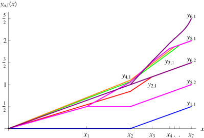
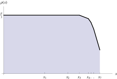
Figure 2: The eigenvalue distribution $y_{a,I}(x)$ (left) for all nodes and density $\rho(x)$ (right) for the $\widehat{D}_{5}$ quiver with CS levels: $(k_{2},k_{3},k_{4},k_{5},k_{6})=(2,2,3,4,4)$.

After a saturation occurs, the total number of independent variables is reduced by one. Thus, at this point, we remove one variable from the Lagrangian, revise the inequalities and solve the equations of motion again until a new saturation is encountered. This process is iterated until all $y_{a}$’s are related, determining a maximum of $(\sum_{a}n_{a}-1)$ regions or until the eigenvalue distribution terminates, $i.e.$, $\rho(x)=0$. Once the eigenvalue density $\rho(x)$ is determined in all regions, the value of $\mu$ (and therefore $F$) is found from the normalization condition (2.3).

The solution to the $\widehat{D}_{4}$ quiver consists of five regions and was solved in [22]. Assuming that $p_{1}\geq p_{2}\geq p_{3}\geq p_{4}\geq 0$, it was found that

$$\frac{1}{\mu^{2}}=-\frac{1}{4p_{1}}+\frac{2p_{1}+3p_{2}-p_{3}}{(p_{1}+p_{2})^{2}}-\frac{1}{2(p_{1}+p_{2}+p_{3}-p_{4})}-\frac{1}{2(p_{1}+p_{2}+p_{3}+p_{4})}\,.$$ (3.2)

We now discuss the solution to the $\widehat{D}_{5}$ quiver, consisting of seven regions. We assume that $k_{6}\geq k_{5}\geq k_{4}\geq k_{3}\geq k_{2}\geq 0$ with $k_{1}=-(k_{2}+k_{3}+k_{4}+2k_{5}+2k_{6})$ implying $p_{1}\geq p_{2}\geq p_{3}\geq p_{4}\geq p_{5}\geq 0$. The solution is summarized in Table 1 and Fig. 2 shows the eigenvalue distributions and density (further details are given in Appendix B).

Region	$x_{i}$	$\delta y(x=x_{i})$	$\rho_{i}(x)$
1	$\frac{\mu}{3(k_{2}+k_{3}+k_{4}+2k_{5}+2k_{6})}$	$y_{1,1}-y_{5,2}=-\frac{1}{2}$	$\frac{1}{3}\mu$
2	$\frac{4\mu}{6k_{2}+9k_{3}+9k_{4}+12k_{5}+18k_{6}}$	$y_{5,2}-y_{6,2}=-\frac{1}{2}$	$\frac{1}{3}\mu$
3	$\frac{2\mu}{3(2k_{2}+k_{3}+k_{4}+2k_{5}+2k_{6})}$	$y_{2,1}-y_{6,2}=0$	$\frac{1}{3}\mu$
4	$\frac{2\mu}{2k_{2}+3(k_{3}+k_{4}+2k_{5}+2k_{6})}$	$y_{5,1}-y_{6,2}=\frac{1}{2}$	$\frac{1}{2}\mu+\frac{1}{4}x(k_{1}-k_{2})$
5	$\frac{2\mu}{2k_{2}+3k_{3}+5k_{4}+4k_{5}+6k_{6}}$	$y_{4,1}-y_{6,2}=\frac{1}{2}$	$\mu+xk_{1}$
6	$\frac{2\mu}{2k_{2}+5k_{3}+3k_{4}+4k_{5}+6k_{6}}$	$y_{3,1}-y_{6,2}=\frac{1}{2}$	$\frac{3}{2}\mu+\frac{1}{4}x(6k_{1}-k_{3}-3k_{4}-2k_{6})$
7	$\frac{2\mu}{2k_{2}+3k_{3}+3k_{4}+4k_{5}+6k_{6}}$	$y_{6,1}-y_{6,2}=1$	$2\mu+x(2k_{1}-k_{3}-k_{4}-k_{6})$

Table 1: Key characteristics of the seven regions of the $\widehat{D}_{5}$ matrix model: their boundaries, the saturated inequalities and the eigenvalue densities, assuming $k_{6}\geq k_{5}\geq k_{4}\geq k_{3}\geq k_{2}\geq 0$.

From the information given in Table 1 and (2.3), we find

$$\frac{1}{\mu^{2}}= -\frac{1}{2k_{2}+5k_{3}+3k_{4}+4k_{5}+6k_{6}}-\frac{1}{2k_{2}+3k_{3}+5k_{4}+4k_{5}+6k_{6}}$$

$$+\frac{4(k_{3}+k_{4}+3k_{6}-2k_{1})}{(2k_{2}+3k_{3}+3k_{4}+4k_{5}+6k_{6})^{2}}$$

$$-\frac{1}{9(2k_{2}+k_{3}+k_{4}+2k_{5}+2k_{6})}-\frac{1}{2k_{2}+3k_{3}+3k_{4}+6k_{5}+6k_{6}}\,,$$

which, using the relations in (2.7) gives

$$\frac{1}{\mu^{2}}= -\frac{1}{18p_{1}}-\frac{1}{2(p_{1}+2p_{2})}+\frac{(2p_{1}+2p_{2}+3p_{3}-p_{4})}{(p_{1}+p_{2}+p_{3})^{2}}$$

$$-\frac{1}{2(p_{1}+p_{2}+p_{3}+p_{4}-p_{5})}-\frac{1}{2(p_{1}+p_{2}+p_{3}+p_{4}+p_{5})}\,.$$ (3.3)

Similarly, solving the $\widehat{D}_{6}$ matrix model as described above leads to a total of nine regions and integrating the eigenvalue density gives

$$\frac{1}{\mu^{2}}= -\frac{1}{48p_{1}}-\frac{1}{6(p_{1}+3p_{2})}-\frac{1}{2(p_{1}+p_{2}+2p_{3})}+\frac{2(p_{1}+p_{2}+p_{3})+3p_{4}-p_{5}}{(p_{1}+p_{2}+p_{3}+p_{4})^{2}}$$

$$-\frac{1}{2(p_{1}+p_{2}+p_{3}+p_{4}+p_{5}-p_{6})}-\frac{1}{2(p_{1}+p_{2}+p_{3}+p_{4}+p_{5}+p_{6})}\,,$$ (3.4)

for $p_{1}\geq p_{2}\geq...\geq p_{6}\geq 0$.

3.2 General Solution and Polygon Area

By comparing (3.2), (3.3) and (3.4), we propose that the free energy for $\widehat{D}_{n}$ quivers is determined by:

$$\frac{1}{\mu^{2}}= \,\frac{1}{2}\sum_{a=1}^{n-3}\frac{c_{a}}{\sum_{b=1}^{a-1}p_{b}+(n-a-1)p_{a}}+\frac{2\sum_{b=1}^{n-3}p_{b}+3p_{n-2}-p_{n-1}}{\left(\sum_{b=1}^{n-2}p_{b}\right)^{2}}$$

$$-\frac{1}{2}\left(\frac{1}{\sum_{b=1}^{n-1}p_{b}-p_{n}}+\frac{1}{\sum_{b=1}^{n}p_{b}}\right),$$ (3.5)

with $c_{a}\equiv\frac{-2}{(n-a-1)(n-a-2)}$ and $p_{1}\geq p_{2}\geq...\geq p_{n}>0$. We have verified that this is correct for the $\widehat{D}_{7},...,\widehat{D}_{10}$ matrix models.

For $\widehat{A}$-quivers, it was shown in [19] that $\text{Vol}(Y)$ can be interpreted as the area of a certain polygon. By rewriting (3.5) in a more suggestive form, we will show that there is a certain polygon (or rather a cone) whose area is related to $\text{Vol}(Y)$ for $\widehat{D}$-quivers as well. This construction will be particularly useful in Sections 5 and 6. We start by observing that the denominators appearing in (3.5) can be written as

$$\bar{\sigma}_{a}=\sum_{b=1}^{n}\left(|p_{a}-p_{b}|+|p_{a}+p_{b}|\right)-4\,|p_{a}|\,;\quad a=1,...,n\,,$$

$$\bar{\sigma}_{0}=2(n-2)\,,\qquad\bar{\sigma}_{n+1}=2\sum_{b=1}^{n}|p_{b}|\,.$$ (3.6)

The first step in rewriting (3.5) is to combine consecutive terms to get

$$\frac{\text{Vol}(Y)}{\text{Vol}(S^{7})}=\frac{1}{2}\left(\frac{1}{\bar{\sigma}_{0}\,\bar{\sigma}_{1}}+\sum_{a=1}^{n-1}\frac{p_{a}-p_{a+1}}{\bar{\sigma}_{a}\,\bar{\sigma}_{a+1}}+\frac{p_{n}}{\bar{\sigma}_{n}\,\bar{\sigma}_{n+1}}\right),$$ (3.7)

where we have used the relation (2.6). The next step is to introduce the vectors $\beta_{a}=(1,p_{a})$ together with $\beta_{0}=(0,1)$ and $\beta_{n+1}=(1,0)$. Defining the wedge product $(a,b)\wedge(c,d)=(ad-bc)$, we can write all the $\bar{\sigma}_{a}$’s in (3.6) in terms of $\gamma_{a,b}\equiv\left|\beta_{a}\wedge\beta_{b}\right|$ as follows

$$\bar{\sigma}_{a}=\sum_{b=1}^{n}\left(\gamma_{a,b}+\gamma_{a,-b}\right)-4\gamma_{a,n+1}\,;\quad a=0,...,n+1\,,$$ (3.8)

where we have also defined $\beta_{-a}\equiv(1,-p_{a})$. This finally leads to

$$\frac{\text{Vol}(Y)}{\text{Vol}(S^{7})}=\frac{1}{2}\sum_{a=0}^{n}\frac{\gamma_{a,a+1}}{\bar{\sigma}_{a}\,\bar{\sigma}_{a+1}}\,.$$ (3.9)

Now, let us consider the vectors $\beta_{a}$, $a=0,...,n+1$ as defining a set of vertices $v_{a}$ given by

$$v_{a}=v_{0}+\textstyle{\sum_{b=0}^{a-1}}\,\beta_{b}\,,$$

where $v_{0}$ is a base point (undetermined for the moment). This set of vertices $v_{a}$ in turn defines a new set of edges by the equations $v_{a}\wedge x=1/2$. Then, the set of intersection points of consecutive edges, given by $w_{a}=\beta_{a}/(2\,v_{a}\wedge v_{a+1})$, together with the origin defines a cone $\mathcal{C}$ whose area is given by

$$\text{Area}(\mathcal{C})=\frac{1}{8}\sum_{a=0}^{n}\frac{\beta_{a+1}\wedge\beta_{a}}{(v_{a}\wedge v_{a+1})(v_{a+1}\wedge v_{a+2})}\,.$$ (3.10)

The denominators $v_{a}\wedge v_{a+1}=v_{a}\wedge(v_{a}+\beta_{a})=v_{a}\wedge\beta_{a}=\left(v_{0}+\textstyle{\sum_{b=0}^{a-1}\beta_{b}}\right)\wedge\beta_{a}$ depend on the choice of base point $v_{0}$. Choosing $v_{0}=(-n+2,-1)$, we can set $(v_{a}\wedge v_{a+1})=-1/2\,\bar{\sigma}_{a}$ leading to

$$\frac{\text{Vol}(Y)}{\text{Vol}(S^{7})}=\text{Area}(\mathcal{C})\,.$$ (3.11)

We also note that by rescaling the cone $\mathcal{C}$ by a factor $2\mu$, we can actually interpret $\rho(x)$ as the height of the cone. In Fig. 3 we show the rescaled cone corresponding to the $\widehat{D}_{5}$ quiver. The $x$ coordinates of the vertices of this cone correspond to the location of the kinks in $\rho(x)$ in Fig. 2. Thus, $1/2=\int dx\,\rho(x)=4\mu^{2}\,\text{Area}(\mathcal{C})$, from where (3.11) follows immediately.

Figure 3: Schematic cone for the $\widehat{D}_{5}$-quiver. The height of the cone gives the density $\rho(x)$ in the regions defined by the $x$ coordinates of the vertices $w_{a}$.

This construction is analogous to the polygon for the $\widehat{A}$-quiver [19]. The vectors $\beta_{a}$ in that case correspond to the $(1,q_{a})$ charges of five-branes involved in the brane description of the theory. The addition of the two extra vectors $\beta_{0}$ and $\beta_{n+1}$ in the present case seems to suggest that one should also include $(0,1)$ and $(1,0)$ branes in the description of these theories.

We would like to comment that solving the matrix model under a different ordering of the $p$’s amounts to permuting them correspondingly in the expression (3.9). Moreover, regardless of the sign and ordering of $p$’s, the denominators appearing in the expression for $\text{Vol}(Y)$ are always given by the $\bar{\sigma}$’s in (3.8). In the next section we will propose a general expression, which is valid for any value of the CS levels and is explicitly invariant under Seiberg duality.

4 General Formula for $\widehat{D}_{n}$ Quivers

It was shown in [23, 24] that the free energy is invariant under a generalized Seiberg duality [25, 26]. For ADE quivers, Seiberg duality can be reinterpreted as the action of the Weyl group, which acts by permuting and changing the sign of an even number of $p$’s in the case of $\widehat{D}$-quivers. Thus, we would like to have an expression for $\text{Vol}(Y)$ that does not assume any particular relation among CS levels and is explicitly invariant under Seiberg duality. It was proposed in [22] that this can be written as a rational function whose numerator is given by $\sum_{\mathcal{R}_{+}}\det(\alpha_{1}...\alpha_{n})^{2}\prod_{a=1}^{n}|\alpha_{a}\cdot p|$, where $\mathcal{R}_{+}$ denotes all $n$-subsets of positive roots. Note that under Weyl transformations the $\bar{\sigma}_{a}$’s defined in (3.8) are simply shuffled among each other. Based on this, we propose that the general expression for the volume corresponding to $\widehat{D}_{n}$ quivers is given by

$$\frac{\text{Vol}(Y)}{\text{Vol}(S^{7})}=\frac{\sum_{\mathcal{R}_{+}}\det(\alpha_{1}...\alpha_{n})^{2}\prod_{a=1}^{n}|\alpha_{a}\cdot p|}{2\prod_{a=0}^{n+1}\bar{\sigma}_{a}}\,.$$ (4.1)

As we will prove below, (4.1) reduces to (3.9) when the CS levels are ordered.

We recall that in the corresponding formula for $\widehat{A}$-quivers, the numerator could be interpreted as a sum over tree graphs [15]. In a similar way, we will show now that the numerator of (4.1) can be interpreted as a sum over certain graphs known as signed graphs [27] (see also [28, 29, 30] and references therein). A graph $\Gamma=(V,E)$ consists of a set of vertices $V$ and a set $E$ of unordered pairs from $V$ (the edges). A signed graph $(\Gamma,\sigma)$ is a graph $\Gamma$ with a signing $\sigma:\,E\rightarrow\{+1,-1\}$ associated to each edge. With these definitions, we can associate a signed graph to each term in the numerator of (4.1). Recall that the roots $\alpha_{a}$ for $D_{n}$ are of the form $\left(e_{i}\pm e_{j}\right)$, where $e_{i}$ are the canonical unit vectors of dimension $n$ and $i\neq j$. To a root of the type $\left(e_{i}-e_{j}\right)$ we associate a positive edge ($\sigma=1$) connecting the nodes $i$ and $j$ in the graph, and to a root of the type $\left(e_{i}+e_{j}\right)$ we associate a negative edge ($\sigma=-1$). Then, we think of the matrix $I=(\alpha_{1}...\,\alpha_{n})$ as an incidence matrix for a diagram with $n$ vertices and $n$ edges. Due to Euler’s theorem, such graphs must contain loops. If the graph contains more than one loop then it must be disconnected. Loops are naturally associated a sign as well, given by the product of the signs of all the edges forming the loop. As we shall explain below, the determinant in (4.1) selects diagrams containing only negative loops. Some examples of diagrams contributing to the numerator for $\widehat{D}_{4}$ are shown in Fig. 4, where dashed lines represent negative edges and solid lines positive ones.

Figure 4: Some signed graphs contributing to the numerator for $\widehat{D}_{4}$. The first diagram, for example, contributes a term $4|(p_{1}+p_{2})(p_{2}-p_{3})(p_{3}-p_{4})(p_{4}-p_{1})|$.

To understand why the determinant vanishes for diagrams with positive loops, it is useful to introduce the operation acting on graphs called ‘switching’. Switching is defined with respect to a vertex $v\in V$, and it acts by reversing the signs of all the edges connected to that vertex. This operation preserves the value of $(\det I)^{2}$ since it corresponds to multiplying some rows and columns of the incidence matrix $I$ by $-1$. It is easy to see that by various switching operations one can turn any loop with an even number of negative edges into a loop made entirely of positive edges. Then, $\text{det}\,I$ will vanish simply because the columns in $I$ associated to these edges add up to zero. On the other hand, if there are an odd number of negative edges in the loop, the above argument does not apply. In fact, one can easily check that $(\det I)^{2}=4$ for each negative loop. Thus, we can also write (4.1) as

$$\frac{\text{Vol}(Y)}{\text{Vol}(S^{7})}=\frac{\sum_{(V,E,\sigma)∈\mathcal{T^{-}}}4^{L_{-}}\prod_{(a,b)\in E}|p_{a}-\sigma p_{b}|}{2\prod_{a=0}^{n+1}\bar{\sigma}_{a}}\,,$$ (4.2)

where $\mathcal{T^{-}}$ denotes the set of signed diagrams with $n$ vertices and $n$ edges (connected or disconnected) and no positive loops, $L_{-}$ is the number of negative loops in the diagram, and $\sigma$ the sign of the corresponding edge. Using a generalized matrix-tree formula, we now show that (4.2) in fact reduces to (3.9) for $p_{a}>p_{a+1}$.

4.1 Generalized Matrix-tree Formula

We define the $n\times n$ adjacency matrix $A$ for a signed graph by:

$$A_{aa}=\sum_{b=1}^{n-1}(\gamma_{a,b}+\gamma_{a,-b})\,,\qquad A_{ab}=-\gamma_{a,b}+\gamma_{a,-b}\,.$$

The generalized matrix-tree formula [29, 30] states that

$$\textstyle{\det A=\sum_{(V,E,\sigma)∈\mathcal{T^{-}}}4^{L_{-}}\prod_{(a,b)\in E}|p_{a}-\sigma p_{b}|}\,.$$ (4.3)

By row and column operations we can bring $A$ into the tri-diagonal form:

$$A=\begin{pmatrix}\bar{\sigma}_{1}+\bar{\sigma}_{2}+2\gamma_{12}&-\bar{\sigma}_{2}&0&\cdots&\cdots&0\\ -\bar{\sigma}_{2}&\bar{\sigma}_{2}+\bar{\sigma}_{3}+2\gamma_{23}&-\bar{\sigma}_{3}&\cdots&\cdots&\vdots\\ 0&-\bar{\sigma}_{3}&\ddots&\ddots&\vdots&\vdots\\ \vdots&\vdots&\ddots&\ddots&-\bar{\sigma}_{n-1}&0\\ \vdots&\cdots&\cdots&-\bar{\sigma}_{n-1}&\bar{\sigma}_{n-1}+\bar{\sigma}_{n}+2\gamma_{n-1,n}&-\bar{\sigma}_{n}\\ 0&\cdots&\cdots&0&-\bar{\sigma}_{n}&\frac{1}{2}\left(\bar{\sigma}_{n}+\bar{\sigma}_{n+1}\right)\end{pmatrix}$$

Using the fact that the determinant of tri-diagonal matrices satisfies a recursion relation, we have

$$\det A=\frac{1}{2}\left(\bar{\sigma}_{n}+\bar{\sigma}_{n+1}\right)\det A_{n-1}-\bar{\sigma}_{n}^{2}\det A_{n-2}\,,$$ (4.4)

$$\det A_{a}=\left(\bar{\sigma}_{a}+\bar{\sigma}_{a+1}+2\gamma_{a,a+1}\right)\det A_{a-1}-\bar{\sigma}_{a}^{2}\det A_{a-2}\,,$$ (4.5)

where $A_{a}$ denotes the $a\times a$ sub-matrix of $A$ for $a=1,...,n-1$. Then, using the identities: $\bar{\sigma}_{a+1}-\bar{\sigma}_{a}=-2(n-2-a)\gamma_{a,a+1}$ and

$$\sum_{d=0}^{a-1}\frac{(n-2-d)\gamma_{d,d+1}}{\bar{\sigma}_{d}\,\bar{\sigma}_{d+1}}=\frac{1}{2\,\bar{\sigma}_{a}}\,,$$

we can show that the recursion relation (4.5) is solved by

$$\det A_{a-1}=\prod_{b=0}^{a}\bar{\sigma}_{b}\,\sum_{d=0}^{a-1}\frac{(a-d)\gamma_{d,d+1}}{\bar{\sigma}_{d}\,\bar{\sigma}_{d+1}}\,.$$ (4.6)

Using (4.6) in (4.4), we have

$$\det A= \,\frac{1}{2}\prod_{b=0}^{n+1}\bar{\sigma}_{b}\,\left[\left(1+\frac{\bar{\sigma}_{n}}{\sigma_{n+1}}\right)\sum_{d=0}^{n-1}\frac{(n-d)\gamma_{d,d+1}}{\bar{\sigma}_{d}\,\bar{\sigma}_{d+1}}-\frac{2\bar{\sigma}_{n}}{\bar{\sigma}_{n+1}}\sum_{d=0}^{n-2}\frac{(n-1-d)\gamma_{d,d+1}}{\bar{\sigma}_{d}\,\bar{\sigma}_{d+1}}\right]$$

$$= \,\frac{1}{2}\prod_{b=0}^{n+1}\bar{\sigma}_{b}\,\sum_{d=0}^{n-1}\left[2\frac{\gamma_{d,d+1}}{\bar{\sigma}_{d}\,\bar{\sigma}_{d+1}}+\left(\frac{\bar{\sigma}_{n+1}-\bar{\sigma}_{n}}{\bar{\sigma}_{n+1}}\right)\frac{(n-2-d)\gamma_{d,d+1}}{\bar{\sigma}_{d}\,\bar{\sigma}_{d+1}}\right]$$

$$= \prod_{b=0}^{n+1}\bar{\sigma}_{b}\,\left[\sum_{d=0}^{n-1}\frac{\gamma_{d,d+1}}{\bar{\sigma}_{d}\,\bar{\sigma}_{d+1}}+\frac{1}{2}\frac{4\gamma_{n,n+1}}{\bar{\sigma}_{n+1}}\frac{1}{2\bar{\sigma}_{n}}\right]$$

$$= \prod_{b=0}^{n+1}\bar{\sigma}_{b}\,\sum_{d=0}^{n}\frac{\gamma_{d,d+1}}{\bar{\sigma}_{d}\,\bar{\sigma}_{d+1}}\,.$$

Finally, substituting (4.3) in (4.2) leads to

$$\frac{\text{Vol}(Y)}{\text{Vol}(S^{7})}=\frac{\det A}{2\prod_{b=0}^{n+1}\bar{\sigma}_{b}}=\frac{1}{2}\sum_{d=0}^{n}\frac{\gamma_{d,d+1}}{\bar{\sigma}_{d}\,\bar{\sigma}_{d+1}}\,,$$

recovering the expression (3.9).

5 Flavored $\widehat{D}_{n}$ Quivers and the F-theorem

The F-Theorem [8] states that the free energy (1.1) decreases along RG flows and is stationary at the RG fixed points of any three-dimensional field theory (supersymmetric or not). Thus, $F$ gives a good measure of the number of degrees of freedom, in analogy with the c-function in two dimensions and the anomaly coefficient, $a$ in four dimensions. This theorem was first tested in a variety of field theories [31, 32, 33] and recently it has been proven in [34, 35] for any three-dimensional field theory by relating $F$ to the entanglement entropy of a disk-like region. Here we check that it holds for the the class of theories we have discussed. We trigger the RG flow by adding massive non-chiral fundamental flavors in the UV. By integrating out non-chiral flavor fields, there is no effective shift in the CS levels. Thus, we are interested in comparing $F(k_{i};n_{F})$ to $F(k_{i};0)$. The addition of $n_{F}\neq 0$ in (2.4) introduces no additional complications and the matrix model is solved as explained in section 3. We solved the flavored $\widehat{D}_{n}$ matrix model for $n=4,...,9$ leading us to

$$\frac{\text{Vol}(Y)}{\text{Vol}(S^{7})}=\frac{1}{2}\left(\frac{\gamma_{01}}{\bar{\sigma}_{0}(\bar{\sigma}_{1}+n_{F})}+\sum_{a=1}^{n}\frac{\gamma_{a,a+1}}{(\bar{\sigma}_{a}+n_{F})(\bar{\sigma}_{a+1}+n_{F})}\right).$$ (5.1)

By comparing (5.1) with (3.9), it is clear that $F(k_{i};n_{F})\geq F(k_{i};0)$ verifying that

$$F_{UV}\geq F_{IR}\,,$$

in accordance with the F-theorem.

In terms of the polygon construction discussed in Section 3.2, adding flavor corresponds to adding the vector $\beta_{F}=(0,n_{F}/2)$ between $\beta_{0}$ and $\beta_{1}$. Then, (5.1) has the same form as (3.9) with $b=F,1,...,n$ in the definition (3.8).

6 Unfolding $\widehat{D}_{n}$ to $\widehat{A}_{2n-5}$

Here we provide a check of the formula (3.9), based on the folding$/$unfolding trick discussed in [36], which relates the free energy of various quiver gauge theories when some CS levels are identified. It can be used to change the gauge groups from unitary to orthosymplectic without changing the quiver or it can be used to change the quiver without changing the type of gauge group. Here we will deal with the latter use, as it relates the free energy of $\widehat{D}$-quivers to that of $\widehat{A}$-quivers.

When the external CS levels of a $\widehat{D}_{n}$ quiver are identified, it can be unfolded to an $\widehat{A}_{2n-5}$ quiver, as shown in Fig. 5. Each internal node in the $\widehat{D}$ quiver is duplicated to give two nodes with the same CS level, while the four external nodes combine to give two nodes with doubled CS levels. Each node in the $\widehat{A}$ quiver corresponds to a $U(2N)$ gauge group and the condition $\sum_{a}n_{a}k_{a}=0$ is automatically satisfied in the unfolded quiver. Using this, it can be shown that in the large $N$ limit, $Z_{D}=\sqrt{Z_{A}}$ and therefore the free energies are related by $F_{D}=\frac{1}{2}F_{A}$. Here we verify explicitly this proportionality by comparing the formula (3.9) to the corresponding formula for $\widehat{A}_{2n-5}$.

Figure 5: Unfolding $\widehat{D}_{n}$ to $\widehat{A}_{2n-5}$. Each node in the $\widehat{A}$ quiver corresponds to a $U(2N)$ gauge group.

Let us first look at the formula for the $\widehat{D}_{n}$ quiver when external CS levels are identified, $i.e.$, $k_{1}=k_{2}=k$ and $k_{3}=k_{4}=k^{\prime}$. Due to the relations in (2.7), this is ensured by setting $p_{1}=p_{n}=0$. Thus, we need the solution to the matrix model with the ordering $p_{2}\geq...\geq p_{n-1}\geq p_{n}\geq p_{1}\geq 0$. As mentioned at the end of Section 3, this is given by permuting the $p$’s in (3.9) accordingly. Then, setting $p_{1}=p_{n}=0$ gives

$$\frac{\text{Vol}(Y_{D})}{\text{Vol}(S^{7})}=\frac{1}{2}\left(\frac{p_{2}}{\bar{\sigma}_{2}^{2}}+\sum_{a=2}^{n-2}\frac{\gamma_{a,a+1}}{\bar{\sigma}_{a}\,\bar{\sigma}_{a+1}}+\frac{p_{n-1}}{(\bar{\sigma}_{n-1})^{2}}\right).$$ (6.1)

Now we wish to compare this expression with the corresponding one for $\widehat{A}_{2n-5}$ [19], namely

$$\frac{\text{Vol}(Y_{A})}{\text{Vol}(S^{7})}=\frac{1}{2}\sum_{a=1}^{2n-4}\frac{\gamma_{a,a+1}}{\sigma_{a}\,\sigma_{a+1}}\,,$$ (6.2)

where $\sigma_{a}=\sum_{a=1}^{2n-4}|q_{a}-q_{b}|$, $\gamma_{a,b}=|q_{a}-q_{b}|$ and $\sum_{a=1}^{2n-4}q_{a}=0$. The identification of opposite CS levels in the $\widehat{A}_{2n-4}$ quiver leads to $q_{a}=-q_{2n-3-a}$ (see Appendix A for details). Then, we assume that $q_{1}\geq...\geq q_{n-2}\geq 0\geq q_{n-1}\geq...\geq q_{2n-4}$ and

$$\sigma_{a}=\sum_{b=1}^{n-2}|q_{a}-q_{b}|+\sum_{b=n-1}^{2n-4}|q_{a}-q_{b}|=\sum_{b=1}^{n-2}(|q_{a}-q_{b}|+|q_{a}+q_{b}|)\,;\quad a=1,...,n-2\,.$$

Noting that $\sigma_{a}=\bar{\sigma}_{a}$ and $q_{a}=p_{a+1}$ for $a=1,...,n-2$, we have

$$\frac{\text{Vol}(Y_{A})}{\text{Vol}(S^{7})}= \,\frac{1}{2}\left(\sum_{a=1}^{n-3}\frac{\gamma_{a,a+1}}{\sigma_{a}\,\sigma_{a+1}}+\frac{\gamma_{n-2,n-1}}{\sigma_{n-2}\,\sigma_{n-1}}+\sum_{a=n-1}^{2n-5}\frac{\gamma_{a,a+1}}{\sigma_{a}\,\sigma_{a+1}}+\frac{\gamma_{2n-4,2n-3}}{\sigma_{2n-4}\,\sigma_{2n-3}}\right)$$

$$= \sum_{a=1}^{n-3}\frac{\gamma_{a,a+1}}{\bar{\sigma}_{a}\,\bar{\sigma}_{a+1}}+\frac{q_{n-2}}{\left(\bar{\sigma}_{n-2}\right)^{2}}+\frac{q_{1}}{\bar{\sigma}_{1}^{2}}$$

$$= \,\frac{p_{2}}{\bar{\sigma}_{2}^{2}}+\sum_{a=2}^{n-2}\frac{\gamma_{a,a+1}}{\bar{\sigma}_{a}\,\bar{\sigma}_{a+1}}+\frac{p_{n-1}}{(\bar{\sigma}_{n-1})^{2}}\,.$$ (6.3)

Thus, comparing (6.3) to (6.1) we have

$$\text{Vol}(Y_{D})=\frac{1}{2}\,\text{Vol}(Y_{A})\,.$$ (6.4)

This relation can also be seen clearly in terms of the areas of the corresponding polygons, as shown in Fig. 6 (the cone as defined in Section 3.2 has been doubled along the dotted line for visual clarity). The outer polygon corresponds to the $\widehat{A}$-quiver with opposite CS levels identified and the shaded region on the left represents the polygon corresponding to a general $\widehat{D}$-quiver; when $p_{1}=p_{n}=0$, this shaded region expands to fill half of the outer polygon on the right.

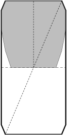
$\xrightarrow{\mathit{Unfolding}}$

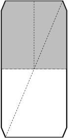
Figure 6: Polygons associated to the $\widehat{D}_{4}$ quiver (shaded region) and $\widehat{A}_{3}$ quiver (outer polygon). Upon unfolding, $\text{Area}(\mathcal{P}_{D})=1/2\,\text{Area}(\mathcal{P}_{A})$.

Recalling that the nodes of the unfolded $\widehat{A}$-quiver correspond to $U(2N)$ gauge groups, we verify that

$$\frac{F_{D}}{F_{A}}=\frac{N^{3/2}}{(2N)^{3/2}}\sqrt{\frac{\text{Vol}(Y_{A})}{\text{Vol}(Y_{D})}}=\frac{1}{2}\,.$$

7 Discussion

In this paper we have studied three-dimensional $\widehat{D}_{n}$ quiver Chern-Simons matter theories by using the localization method of Kapustin, Willet and Yaakov in the large $N$ limit. These field theories are believed to be dual to M-theory on $AdS_{4}\times Y$, where $Y$ is a tri-Sasaki Einstein manifold. We have explicitly solved the corresponding matrix models for various values of $n$, leading us to conjecture a general expression for the free energy and therefore for the volume of the corresponding space $Y$ given in (4.1). We have shown that the numerator of this expression can be interpreted as a sum over a class of graphs with edges that carry a sign, known as signed graphs. Using a generalized matrix-tree formula, we prove that for a particular ordering of CS levels, it can also be interpreted as the area of a certain polygon, given by (3.9). When external CS levels in the $\widehat{D}_{n}$ quiver are identified, the area of this polygon becomes half the area of the polygon corresponding to the $\widehat{A}_{2n-5}$ quiver, in accordance with the unfolding procedure. We have also studied the addition of massive flavor fields, showing that when they are integrated out, the area of the corresponding polygon always increases (thereby decreasing $F$), in accordance with the F-theorem.

The relevant tri-Sasaki Einstein space for a $\widehat{D}_{n}$ quiver is the base of the hyperkähler cone defined by the quotient $\mathbb{H}^{4n-8}///U(1)^{n-1}\times SU(2)^{n-3}$. To the best of our knowledge, the volumes of these spaces have not been computed. Thus, (4.1) can be considered as an AdS/CFT prediction for these volumes. A possible approach to proving the conjectured expression for the free energy would be to find the general solution to the matrix model, perhaps in terms of the polygon construction presented above, as it has been done for the $\widehat{A}$-quiver in [19]. Some questions which have not been addressed here are whether there is a group theory interpretation of the volume formula and whether its denominator can be written in a form that is universal for any ADE quiver.

Appendix A Roots of $\widehat{A}_{m-1}$ and $\widehat{D}_{n}$

Here we give some useful information about the roots for $\widehat{A}$ and $\widehat{D}$ Lie algebras. For $\widehat{A}_{m-1}$ we choose the following root basis

$$\tilde{\alpha}_{a}=e_{a}-e_{a+1}\,,\quad a=1,...,m-1\,;\qquad\tilde{\theta}=-e_{1}+e_{m}\,,$$

where $e_{a}$ are canonical unit vectors of dimension $m$. For $\widehat{D}_{n}$ we choose

$$\alpha_{i}=e_{i}-e_{i+1}\,,\quad i=1,...,n-1\,;\qquad\alpha_{n}=e_{n-1}+e_{n}\,,\qquad\theta=-(e_{1}+e_{2})\,,$$

where $e_{i}$ are the unit vectors of dimension $n$.

Figure 7: Dynkin diagrams for $\widehat{A}_{2n-5}$ and $\widehat{D}_{n}$.

In Fig. 7 we show the affine Dynkin diagrams for the $\widehat{A}$ and $\widehat{D}$ Lie algebras along with the roots associated with every node. At each node, the CS level is given by $\tilde{\alpha}\cdot q$ and $\alpha\cdot p$ for $\widehat{A}$ and $\widehat{D}$, respectively. The identification of opposite CS levels in the $\widehat{A}_{2n-5}$ quiver imposes $\tilde{\alpha}_{a}\cdot q=\tilde{\alpha}_{2n-4-a}\cdot q$ and hence $q_{a}=-q_{2n-3-a}$ for $a=1,...,n-2$. With these conventions, unfolding the $\widehat{D}$-quiver to the $\widehat{A}$-quiver relates $q_{a}=p_{a+1}$.

Appendix B $\widehat{D}_{5}$

Here we give the detailed solution of the matrix model for the $\widehat{D}₅$ quiver gauge theory. As discussed in Section 3, there are 7 regions defining a generic solution of this model. To keep the notation simple, the second index for the four $y$’s corresponding to the external nodes is suppressed.

Region 1: $0\leq x\leq\frac{\mu}{3(k_{2}+k_{3}+k_{4}+2k_{5}+2k_{6})}$

$$\rho=\frac{\mu}{3}\,;$$

$$y_{1}-y_{6,2}=\frac{\left(2k_{1}-k_{3}-k_{4}-2k_{6}\right)x}{4\rho}\,,\quad y_{2}-y_{6,2}=\frac{\left(2k_{2}-k_{3}-k_{4}-2k_{6}\right)x}{4\rho}\,,\quad y_{3}-y_{6,2}=\frac{k_{3}x}{2\rho}\,,$$

$$y_{4}-y_{6,2}=\frac{k_{4}x}{2\rho}\,,\quad y_{5,1}-y_{6,2}=y_{5,2}-y_{6,2}=-\frac{(k_{3}+k_{4}+2k_{6})x}{4\rho}\,,\quad y_{6,1}-y_{6,2}=0\,.$$

Region 2: $\frac{\mu}{3(k_{2}+k_{3}+k_{4}+2k_{5}+2k_{6})}\leq x\leq\frac{4\mu}{6k_{2}+9k_{3}+9k_{4}+12k_{5}+18k_{6}}$

$$\rho=\frac{\mu}{3}\,;$$

$$y_{1}-y_{5,2}=-\frac{1}{2}\,,\quad y_{2}-y_{6,2}=\frac{\left(2k_{2}-k_{3}-k_{4}-2k_{6}\right)x}{4\rho}\,,\quad y_{3}-y_{6,2}=\frac{k_{3}x}{2\rho}\,,$$

$$y_{4}-y_{6,2}=\frac{k_{4}x}{2\rho}\,,\quad y_{5,1}-y_{6,2}=-\frac{1}{2}-\frac{\left(2k_{1}+k_{3}+k_{4}+2k_{6}\right)x}{4\rho}\,,$$

$$y_{5,2}-y_{6,2}=\frac{1}{2}+\frac{\left(2k_{1}-k_{3}-k_{4}-2k_{6}\right)x}{4\rho}\,,\quad y_{6,1}-y_{6,2}=0\,.$$

Region 3: $\frac{4\mu}{6k_{2}+9k_{3}+9k_{4}+12k_{5}+18k_{6}}\leq x\leq\frac{2\mu}{3(2k_{2}+k_{3}+k_{4}+2k_{5}+2k_{6})}$

$$\rho=\frac{\mu}{3}\,;$$

$$y_{1}-y_{5,2}=-\frac{1}{2}\,,\quad y_{2}-y_{6,2}=-1-\frac{\left(k_{1}-k_{2}\right)x}{2\rho}\,,\quad y_{3}-y_{6,2}=-1-\frac{\left(2k_{1}-3k_{3}-k_{4}-2k_{6}\right)x}{4\rho}\,,$$

$$y_{4}-y_{6,2}=-1-\frac{\left(2k_{1}-k_{3}-3k_{4}-2k_{6}\right)x}{4\rho}\,,\quad y_{5,1}-y_{6,2}=-\frac{3}{2}-\frac{k_{1}x}{\rho}\,,$$

$$y_{5,2}-y_{6,2}=-\frac{1}{2}\,,\quad y_{6,1}-y_{6,2}=-2-\frac{\left(2k_{1}-k_{3}-k_{4}-2k_{6}\right)x}{2\rho}\,.$$

Region 4: $\frac{2\mu}{3(2k_{2}+k_{3}+k_{4}+2k_{5}+2k_{6})}\leq x\leq\frac{2\mu}{2k_{2}+3(k_{3}+k_{4}+2k_{5}+2k_{6})}$

$$\rho=\frac{\mu}{2}+\frac{x}{4}\left(k_{1}-k_{2}\right)\,;$$

$$y_{1}-y_{5,2}=-\frac{1}{2}\,,\quad y_{2}-y_{6,2}=0\,,\quad y_{3}-y_{6,2}=-\frac{1}{2}+\frac{\left(2k_{3}+k_{4}+k_{5}+2k_{6}\right)x}{2\rho}\,,$$

$$y_{4}-y_{6,2}=-\frac{1}{2}+\frac{\left(k_{3}+2k_{4}+k_{5}+2k_{6}\right)x}{2\rho}\,,\quad y_{5,1}-y_{6,2}=-\frac{1}{2}-\frac{\left(k_{1}-k_{2}\right)x}{2\rho}\,,$$

$$y_{5,2}-y_{6,2}=-\frac{1}{2}\,,\quad y_{6,1}-y_{6,2}=-1+\frac{\left(k_{3}+k_{4}+k_{5}+2k_{6}\right)x}{\rho}\,.$$

Region 5: $\frac{2\mu}{2k_{2}+3(k_{3}+k_{4}+2k_{5}+2k_{6})}\leq x\leq\frac{2\mu}{2k_{2}+3k_{3}+5k_{4}+4k_{5}+6k_{6}}$

$$\rho=\mu+xk_{1}\,;$$

$$y_{1}-y_{5,2}=-\frac{1}{2}\,,\quad y_{2}-y_{6,2}=0\,,\quad y_{3}-y_{6,2}=\frac{\left(3k_{3}+k_{4}+2k_{6}\right)x}{4\rho}\,,$$

$$y_{4}-y_{6,2}=\frac{\left(k_{3}+3k_{4}+2k_{6}\right)x}{4\rho}\,,\quad y_{5,1}-y_{6,2}=\frac{1}{2}\,,$$

$$y_{5,2}-y_{6,2}=-\frac{1}{2}\,,\quad y_{6,1}-y_{6,2}=\frac{\left(k_{3}+k_{4}+2k_{6}\right)x}{2\rho}\,.$$

Region 6: $\frac{2\mu}{2k_{2}+3k_{3}+5k_{4}+4k_{5}+6k_{6}}\leq x\leq\frac{2\mu}{2k_{2}+5k_{3}+3k_{4}+4k_{5}+6k_{6}}$

$$\rho=\frac{3\mu}{2}+\frac{x}{4}\left(6k_{1}-k_{3}-3k_{4}-2k_{6}\right)\,;$$

$$y_{1}-y_{5,2}=-\frac{1}{2}\,,\quad y_{2}-y_{6,2}=0\,,\quad y_{3}-y_{6,2}=\frac{1}{6}+\frac{\left(2k_{3}+k_{6}\right)x}{3\rho}\,,$$

$$y_{4}-y_{6,2}=\frac{1}{2}\,,\quad y_{5,1}-y_{6,2}=\frac{1}{2}\,,\quad y_{5,2}-y_{6,2}=-\frac{1}{2}\,,\quad y_{6,1}-y_{6,2}=\frac{1}{3}+\frac{\left(k_{3}+2k_{6}\right)x}{3\rho}\,.$$

Region 7: $\frac{2\mu}{2k_{2}+5k_{3}+3k_{4}+4k_{5}+6k_{6}}\leq x\leq\frac{2\mu}{2k_{2}+3k_{3}+3k_{4}+4k_{5}+6k_{6}}$

$$\rho=2\mu+x\left(2k_{1}-k_{3}-k_{4}-k_{6}\right)\,;$$

$$y_{1}-y_{5,2}=-\frac{1}{2}\,,\quad y_{2}-y_{6,2}=0\,,\quad y_{3}-y_{6,2}=\frac{1}{2}\,,\quad y_{4}-y_{6,2}=\frac{1}{2}\,,$$

$$y_{5,1}-y_{6,2}=\frac{1}{2}\,,\quad y_{5,2}-y_{6,2}=-\frac{1}{2}\,,\quad y_{6,1}-y_{6,2}=\frac{1}{2}+\frac{k_{6}x}{2\rho}\,.$$

Finally, the last saturation occurs at the end of this region with $y_{6,1}=y_{6,2}+1$.

Appendix C Exceptional Quivers

We have also solved the matrix models for the exceptional quivers $\widehat{E}_{6},\widehat{E}_{7}$ and $\widehat{E}_{8}$. They consist of eleven, seventeen and twenty-nine regions respectively. Here we give the corresponding free energies for a particular ordering of the CS levels. In Fig. 8, we show our conventions in labeling the nodes.

Figure 8: Labeling of Chern-Simons levels for $\widehat{E}_{6},\widehat{E}_{7}$ and $\widehat{E}_{8}$.

$\widehat{E}_{6}$

The matrix model for $\widehat{E}_{6}$ gives:

$$\frac{2}{\mu^{2}}= \frac{2(4k_{2}+11k_{3}+8k_{4}+4k_{5}+6k_{6}+4k_{7})}{(2k_{2}+5k_{3}+4k_{4}+2k_{5}+3k_{6}+2k_{7})^{2}}-\frac{1}{42(3k_{2}+6k_{3}+4k_{4}+2k_{5}+5k_{6}+k_{7})}$$

$$-\frac{1}{77(13k_{2}+12k_{3}+8k_{4}+4k_{5}+3k_{6}+2k_{7})}-\frac{1}{3(3k_{2}+6k_{3}+4k_{4}+2k_{5}+5k_{6}+4k_{7})}$$

$$-\frac{9}{6k_{2}+14k_{3}+13k_{4}+6k_{5}+9k_{6}+6k_{7}}-\frac{9}{11(6k_{2}+14k_{3}+13k_{4}+12k_{5}+9k_{6}+6k_{7})}\,,$$

under the assumptions that $k_{6}\geq k_{5}\geq k_{4}\geq k_{3}\geq k_{2}\geq 0$ and $k_{7}>3k_{2}+6k_{3}+4k_{4}+2k_{5}+4k_{6}$.

$\widehat{E}_{7}$

The matrix model for $\widehat{E}_{7}$ gives:

$$\frac{2}{\mu^{2}}= \frac{8k_{2}+24k_{3}+42k_{4}+4(8k_{5}+6k_{6}+3k_{7}+5k_{8})}{(2k_{2}+6k_{3}+10k_{4}+8k_{5}+6k_{6}+3k_{7}+5k_{8})^{2}}$$

$$-\frac{1}{2k_{2}+7k_{3}+10k_{4}+8k_{5}+6k_{6}+3k_{7}+5k_{8}}-\frac{1}{2k_{2}+6k_{3}+10k_{4}+9k_{5}+6k_{6}+3k_{7}+5k_{8}}$$

$$-\frac{1}{180(2k_{2}+3k_{3}+4k_{4}+3k_{5}+2k_{6}+k_{7}+2k_{8})}$$

$$-\frac{4}{15(4k_{2}+11k_{3}+2(9k_{4}+8k_{5}+7k_{6}+6k_{7})+9k_{8})}$$

$$-\frac{27}{7(6k_{2}+17k_{3}+28k_{4}+24k_{5}+20k_{6}+9k_{7}+15k_{8})}$$

$$-\frac{32}{21(8k_{2}+25k_{3}+42k_{4}+32k_{5}+22k_{6}+12k_{7}+27k_{8})}\,,$$

under the assumptions that $k_{7}\geq k_{6}\geq k_{5}\geq k_{4}\geq k_{3}\geq k_{2}\geq 0$ along with $4k_{3}+k_{4}>2k_{5}+k_{6}\,,k_{3}+2k_{4}+k_{5}>k_{7}\,,k_{4}+k_{5}>k_{6}\,\,\text{and}\,\,3k_{8}>6k_{3}+12k_{4}+15k_{5}+10k_{6}+5k_{7}$.

$\widehat{E}_{8}$

The solution of the matrix model for $\widehat{E}_{8}$ gives:

$$\frac{2}{\mu^{2}}= \frac{8k_{2}+24k_{3}+48k_{4}+74k_{5}+92k_{6}+48k_{7}+64k_{8}+32k_{9}}{(2k_{2}+6k_{3}+12k_{4}+18k_{5}+23k_{6}+12k_{7}+16k_{8}+8k_{9})^{2}}$$

$$-\frac{1}{3150(2k_{2}+3k_{3}+4k_{4}+5k_{5}+6k_{6}+3k_{7}+4k_{8}+2k_{9})}$$

$$-\frac{1}{2(k_{2}+3k_{3}+6k_{4}+9k_{5}+12k_{6}+6k_{7}+8k_{8}+4k_{9})}$$

$$-\frac{1}{2k_{2}+6k_{3}+13k_{4}+18k_{5}+23k_{6}+12k_{7}+16k_{8}+8k_{9}}$$

$$-\frac{27}{7(6k_{2}+18k_{3}+35k_{4}+52k_{5}+69k_{6}+38k_{7}+48k_{8}+24k_{9})}$$

$$-\frac{108}{35(12k_{2}+36k_{3}+70k_{4}+104k_{5}+138k_{6}+69k_{7}+103k_{8}+48k_{9})}$$

$$-\frac{36}{55(12k_{2}+36k_{3}+70k_{4}+104k_{5}+138k_{6}+69k_{7}+103k_{8}+68k_{9})}$$

$$-\frac{9}{154(6k_{2}+17(3k_{3}+4k_{4}+5k_{5}+6k_{6}+3k_{7}+4k_{8}+2k_{9}))}\,,$$

assuming that $k_{6}\geq k_{5}\geq k_{4}\geq k_{3}\geq k_{2}\geq 0\,,k_{7}>3k_{4}+6k_{5}+4k_{6}\,,2k_{4}+4k_{5}+6k_{6}+9k_{7}>k_{8}\,,2k_{3}+4k_{4}+6k_{5}+8k_{6}+4k_{7}+6k_{8}>k_{9}\,\,\text{and}\,\,2k_{9}>6k_{3}+12k_{4}+18k_{5}+24k_{6}+16k_{7}+11k_{8}$.

References

- [1] E. Witten, “Topological Quantum Field Theory”, Commun. Math. Phys. 117 (1988) 353.
- [2] V. Pestun, “Localization of Gauge Theory on a Four-sphere and Supersymmetric Wilson Loops”, Commun. Math. Phys. 313 (2012) 71 [arXiv:0712.2824 [hep-th]].
- [3] A. Kapustin, B. Willett and I. Yaakov, ‘‘Exact Results for Wilson Loops in Superconformal Chern-Simons Theories with Matter’’, JHEP 1003 (2010) 089 [arXiv:0909.4559 [hep-th]].
- [4] D. L. Jafferis, ‘‘The Exact Superconformal R-Symmetry Extremizes Z’’, JHEP 1205 (2012) 159 [arXiv:1012.3210 [hep-th]].
- [5] N. Hama, K. Hosomichi and S. Lee, ‘‘Notes on SUSY Gauge Theories on Three-Sphere’’, JHEP 1103 (2011) 127 [arXiv:1012.3512 [hep-th]].
- [6] J. Kallen and M. Zabzine, ‘‘Twisted Supersymmetric 5D Yang-Mills Theory and Contact Geometry’’, JHEP 1205 (2012) 125 [arXiv:1202.1956 [hep-th]].
- [7] D. L. Jafferis and S. S. Pufu, ‘‘Exact Results for Five-dimensional Superconformal Field Theories with Gravity Duals’’, 2012, arXiv:1207.4359 [hep-th].
- [8] D. L. Jafferis, I. R. Klebanov, S. S. Pufu and B. R. Safdi, ‘‘Towards the F-Theorem: N=2 Field Theories on the Three-Sphere’’, JHEP 1106 (2011) 102 [arXiv:1103.1181 [hep-th]].
- [9] J. M. Maldacena, ‘‘The Large N Limit of Superconformal Field Theories and Supergravity’’, Adv. Theor. Math. Phys. 2 (1998) 231 [arXiv:hep-th/9711200].
- [10] S. S. Gubser, I. R. Klebanov and A. M. Polyakov, ‘‘Gauge Theory Correlators from Noncritical String Theory’’, Phys. Lett. B 428 (1998) 105 [arXiv:hep-th/9802109].
- [11] E. Witten, ‘‘Anti-de Sitter Space and Holography’’, Adv. Theor. Math. Phys. 2 (1998) 253 [arXiv:hep-th/9802150].
- [12] N. Drukker, M. Marino and P. Putrov, ‘‘From Weak to Strong Coupling in ABJM Theory’’, Commun. Math. Phys. 306 (2011) 511 [arXiv:1007.3837 [hep-th]].
- [13] O. Aharony, O. Bergman, D. L. Jafferis and J. Maldacena, ‘‘N=6 Superconformal Chern-Simons-matter Theories, M2-branes and their Gravity Duals’’, JHEP 0810 (2008) 091 [arXiv:0806.1218 [hep-th]].
- [14] I. R. Klebanov and A. A. Tseytlin, ‘‘Entropy of Near Extremal Black p-branes’’, Nucl. Phys. B 475 (1996) 164 [arXiv:hep-th/9604089].
- [15] C. P. Herzog, I. R. Klebanov, S. S. Pufu and T. Tesileanu, ‘‘Multi-Matrix Models and Tri-Sasaki Einstein Spaces’’, Phys. Rev. D 83 (2011) 046001 [arXiv:1011.5487 [hep-th]].
- [16] D. Martelli and J. Sparks, ‘‘The Large N Limit of Quiver Matrix Models and Sasaki-Einstein Manifolds’’, Phys. Rev. D 84 (2011) 046008 [arXiv:1102.5289 [hep-th]].
- [17] S. Cheon, H. Kim and N. Kim, ‘‘Calculating the Partition Function of N=2 Gauge Theories on and AdS/CFT Correspondence’’, JHEP 1105 (2011) 134 [arXiv:1102.5565 [hep-th]].
- [18] D. L. Jafferis and A. Tomasiello, ‘‘A Simple Class of N=3 Gauge/Gravity Duals’’, JHEP 0810 (2008) 101 [arXiv:0808.0864 [hep-th]].
- [19] D. R. Gulotta, C. P. Herzog and S. S. Pufu, ‘‘From Necklace Quivers to the F-theorem, Operator Counting, and T(U(N))’’, JHEP 1112 (2011) 077 [arXiv:1105.2817 [hep-th]].
- [20] H.-U. Yee, ‘‘AdS/CFT with Tri-Sasakian Manifolds’’, Nucl. Phys. B 774 (2007) 232 [arXiv:hep-th/0612002].
- [21] B. Assel, C. Bachas, J. Estes and J. Gomis, ‘‘IIB Duals of D=3 N=4 Circular Quivers’’, 2012, arXiv:1210.2590 [hep-th].
- [22] D. R. Gulotta, J. P. Ang and C. P. Herzog, ‘‘Matrix Models for Supersymmetric Chern-Simons Theories with an ADE Classification’’, JHEP 1201 (2012) 132 [arXiv:1111.1744 [hep-th]].
- [23] B. Willett and I. Yaakov, ‘‘N=2 Dualities and Z Extremization in Three Dimensions’’, 2011, arXiv:1104.0487 [hep-th].
- [24] F. Benini, C. Closset and S. Cremonesi, ‘‘Comments on 3d Seiberg-like Dualities’’, JHEP 1110 (2011) 075 [arXiv:1108.5373 [hep-th]].
- [25] O. Aharony, ‘‘IR Duality in d=3 N=2 Supersymmetric USp(2N(c)) and U(N(c)) Gauge Theories’’, Phys. Lett. B 404 (1972) 71 [arXiv:hep-th/9703215].
- [26] A. Giveon and D. Kutasov, ‘‘Seiberg Duality in Chern-Simons Theory’’, Nucl. Phys. B 812 (2009) 1 [arXiv:0808.0360 [hep-th]].
- [27] F. Harary, ‘‘On the Notion of Balance of a Signed Graph’’, Michigan Math. J. 2 (1953-54) 143.
- [28] Thomas Zaslavsky, ‘‘The Geometry of Root Systems and Signed Graphs’’, The American Math. Monthly 88 (1981) 88.
- [29] Thomas Zaslavsky, ‘‘Signed Graphs’’, Discrete Applied Math. 4 (1982) 47.
- [30] Seth Chaiken, ‘‘A Combinatorial Proof of the All Minors Matrix Tree Theorem’’, SIAM. J. on Algebraic and Discrete Methods, 3 (1982) 319.
- [31] I. R. Klebanov, S. S. Pufu and B. R. Safdi, ‘‘F-Theorem Without Supersymmetry’’, JHEP 1110 (2011) 038 [arXiv:1105.4598 [hep-th]].
- [32] A. Amariti and M. Siani, ‘‘Z-extremization and F-theorem in Chern-Simons Matter Theories’’, JHEP 1110 (2011) 016 [arXiv:1105.0933 [hep-th]].
- [33] I. R. Klebanov, S. S. Pufu, S. Sachdev and B. R. Safdi, ‘‘Entanglement Entropy of 3-d Conformal Gauge Theories with Many Flavors’’, JHEP 1205 (2012) 036 [arXiv:1112.5342 [hep-th]].
- [34] H. Casini, M. Huerta and R. C. Myers, ‘‘Towards a Derivation of Holographic Entanglement Entropy’’, JHEP 1105 (2011) 036 [arXiv:1102.0440 [hep-th]].
- [35] H. Casini and M. Huerta, ‘‘On the RG Running of the Entanglement Entropy of a Circle’’, Phys. Rev. D 85 (2012) 125016 [arXiv:1202.5650 [hep-th]].
- [36] D. R. Gulotta, C. P. Herzog and T. Nishioka, ‘‘The ABCDEF’s of Matrix Models for Supersymmetric Chern-Simons Theories’’, JHEP 1204 (2012) 138 [arXiv:1201.6360 [hep-th]].