The Redshift–Space Cluster–Galaxy Cross–Correlation Function: I. Modeling Galaxy Infall onto Millennium Simulation Clusters and SDSS Groups

Abstract

The large scale infall of galaxies around massive clusters provides a potentially powerful diagnostic of structure growth, dark energy, and cosmological deviations from General Relativity. We develop and test a method to recover galaxy infall kinematics (GIK) from measurements of the redshift–space cluster–galaxy cross–correlation function $\xi^{s}_{cg}(r_{p},r_{\pi})$. Using galaxy and halo samples from the Millennium simulation, we calibrate an analytic model of the galaxy kinematic profiles comprised of a virialized component with an isotropic Gaussian velocity distribution and an infall component described by a skewed 2D $t$-distribution with a characteristic infall velocity $v_{r,c}$ and separate radial and tangential dispersions. We show that convolving the real-space cross-correlation function with this velocity distribution accurately predicts the redshift-space $\xi^{s}_{cg}$, and we show that measurements of $\xi^{s}_{cg}$ can be inverted to recover the four distinct elements of the GIK profiles. These in turn provide diagnostics of cluster mass profiles, and we expect the characteristic infall velocity $v_{r,c}(r)$ in particular to be insensitive to galaxy formation physics that can affect velocity dispersions within halos. As a proof of concept we measure $\xi^{s}_{cg}$ for rich galaxy groups in the Sloan Digital Sky Survey and recover GIK profiles for groups in two bins of central galaxy stellar mass. The higher mass bin has a $v_{r,c}(r)$ curve very similar to that of $10^{14}\,h^{-1}M_{\odot}$ halos in the Millennium simulation, and the recovered kinematics follow the expected trends with mass. GIK modeling of cluster–galaxy cross–correlations can be a valuable complement to stacked weak lensing analyses, allowing novel tests of modified gravity theories that seek to explain cosmic acceleration.

1 Introduction

As the largest bound systems in the universe, galaxy clusters carry imprints of cosmic growth via the distribution and motion of their surrounding dark matter and galaxies (see Allen et al., 2011; Kravtsov & Borgani, 2012, and references within). They can therefore play a powerful role in testing theories for the origin of cosmic acceleration, complementing geometrical probes such as supernovae and baryon acoustic oscillations. The key uncertainty in this approach is calibration of the relation between cluster observables (e.g., X-ray luminosity or temperature, optical galaxy richness, Sunyaev–Zel’dovich decrement) and halo mass. Stacked weak lensing has emerged as a robust approach to this problem because it is unaffected by the baryonic physics of the intracluster gas (Mandelbaum et al. 2006; Sheldon et al. 2009; Oguri et al. 2012, see Weinberg et al. 2012 for a review of this approach in the broader context of dark energy studies). Galaxy infall patterns (Gunn & Gott, 1972; Ryden & Gunn, 1987; Regos & Geller, 1989) offer an alternative probe of cluster mass profiles, which may prove a valuable complement to weak lensing if it can be implemented in a way that is insensitive to uncertainties of galaxy formation physics. The redshift–space cluster–galaxy cross–correlation function, $\xi^{s}_{cg}$, is a comprehensive characterization of the statistical relation between clusters and galaxies, influenced by both the real–space cross–correlation and the peculiar velocities induced by the cluster gravitational potential. This paper is the first of a three-part series which will describe the modeling of $\xi^{s}_{cg}$ and investigate its diagnostic power for cluster mass calibration and constraining cosmology.

In cluster–centric coordinates, the average galaxy kinematics are the result of competition between the cluster potential and Hubble expansion. At small distances, virial motion dominates, making the galaxy distribution elongated along the line-of-sight (LOS) direction (a.k.a. the “Fingers-of-God” effect; FOG) (Jackson, 1972). At larger distances, the galaxy kinematics become dominated by radial infall, with a typical turn–around radius of several $h^{-1}\mathrm{Mpc}$, where the characteristic infall velocity is equal to the Hubble flow. This coherent infall produces a squashing distortion in $\xi^{s}_{cg}$ at large scales, often referred to as the Kaiser effect (Kaiser 1987; see also Sargent & Turner 1977). These two redshift space distortion (RSD) effects (see Hamilton 1998 for a pedagogical review) are also seen in the redshift–space galaxy auto–correlation functions (e.g., Reid et al., 2012, and references within), but since galaxies feel a much stronger central potential near clusters than in the field, both small scale dispersion and large scale infall are strongly enhanced in the $\xi^{s}_{cg}$ case.

The strong RSD in $\xi^{s}_{cg}$ allows reconstruction of the average galaxy kinematics around clusters, which are in turn determined by the average cluster mass profiles. For clusters of fixed mass $M$, $\xi^{s}_{cg}(r_{p},r_{\pi})$ at projected separation $r_{p}$ and LOS separation $r_{\pi}$ can be derived by convolving the real–space cross–correlation function $\xi^{r}_{cg}$ with the LOS velocity distribution function $f(v_{\mathrm{los}}|r_{p},y)$ (Peebles, 1980; Fisher, 1995),

$$\xi^{s}_{cg}(r_{p},r_{\pi})+1=\left[\xi^{r}_{cg}\left(\sqrt{r_{p}^{2}+y^{2}}\right)+1\right]\ast f(v_{\mathrm{los}}|r_{p},y),$$ (1)

where $y$ is the LOS separation in real space. The real–space $\xi^{r}_{cg}$ has a roughly power–law form, so the strongest features in $\xi^{s}_{cg}$ arise largely from $f(v_{\mathrm{los}}|r_{p},y)$. In this paper, we first develop an analytic description of the average galaxy infall kinematics (GIK) around cluster–mass halos found in the Millennium simulation (Springel, 2005). We show that applying this model to Equation 1 accurately reproduces the simulated $\xi^{s}_{cg}$, and we show that the analysis can be reversed to infer the correct GIK from measurements of $\xi^{s}_{cg}(r_{p},r_{\pi})$. As an illustrative application to observed data, we measure $\xi^{s}_{cg}$ for galaxy groups (Yang et al., 2007) identified in the Sloan Digital Sky Survey (SDSS; York et al. 2000) and apply our model to infer the infall kinematics.

At small scales, the redshift–space distribution of $\xi^{s}_{cg}$ depends mainly on the velocity dispersion profile of the virialized cluster component. At large separations, one must consider the mean radial velocity profile and the profiles of radial and tangential velocity dispersions. (In fact, we will show that the velocity distributions are significantly non–Gaussian and exhibit internal correlations, all of which must be modeled to describe $\xi^{s}_{cg}$ accurately.) All four of these profiles can be reconstructed from our $\xi^{s}_{cg}$ modeling techniques, and all four of them provide diagnostics of cluster mass. We are particularly hopeful that the mean radial flow will prove to be a tool for inferring average mass profiles that is insensitive to galaxy formation physics. The cluster velocity dispersion profile can be affected at the $10\--20\%$ level by orbital anisotropy and potentially by other effects such as preferential destruction of galaxies that pass near the cluster center or incomplete relaxation of substructures. The velocity dispersions of galaxies within infalling halos may also be affected by biases arising from galaxy formation physics. However, the mean velocity of galaxies in an infalling halo should, on average, match the mean velocity of the halo itself, as galaxies and dark matter are affected by the same gravitational potential. We will test this conjecture in future work.

Figure 1: Three representations of the average galaxy distribution around Millennium clusters with mass between $1.259-1.585\times 10^{14}M_{\odot}$ in the redshift–projected separation plane. Left panel: Number of stacked galaxies in $r_{p}$-$c\Delta z$ cells. Middle panel: Cluster–galaxy correlation function in redshift space $\xi^{s}_{cg}$. Right panel: $\xi^{s}_{cg}$ normalized by the projected cluster–galaxy correlation function $w_{p}$ at each $r_{p}$. The yellow solid U-shape curve delineates the characteristic scale of $r_{\pi}$ at which $\xi^{s}_{cg}$ drops by one e–fold at fixed $r_{p}$, relative to its value at $r_{\pi}=0$. The contour levels for each panel are colour–coded by the top colour bar.

Around individual clusters, the galaxy distribution in the ($r_{p}$, $r_{\pi}$) plane shows a distinctive trumpet–shaped pattern, and the distribution in $r_{\pi}$ at fixed $r_{p}$ often shows a caustic–like discontinuity (Diaferio & Geller, 1997). N-body simulations suggest that the caustic location provides a direct measure of the escape velocity profile, which can in turn be converted to a cluster mass profile (Diaferio 1999; see Serra et al. 2011 for the current state of the art). Rines et al. (2003) have used this technique to infer cluster mass profiles extending beyond the virial radius (also see Rines & Diaferio, 2006; Geller et al., 2012; Rines et al., 2012). However, measurements for any individual cluster are affected by galaxy shot noise and by departures from spherical symmetry (White et al., 2010), and it is not clear whether averaging measurements from multiple clusters will yield an unbiased mean result. Our initial motivation for this study was, in part, to generalize the “caustic method” to the case where an overlapping cluster survey and galaxy redshift survey provide a large total number of cluster–galaxy pairs, even though the numbers around an individual cluster may be too small for caustic detection. Although we will draw connections between $\xi^{s}_{cg}$ and the trumpet–shaped patterns of the caustic method, our approach ultimately does not rely on finding discontinuities in the data or identifying them with the escape velocity profile. Instead it relies on the general predictions of velocity distributions around massive halos in cosmological N-body simulations. Previous analyses of $\xi^{s}_{cg}$ include the study of Croft et al. (1999) using APM galaxy clusters and the study of Li et al. (2012) using velocity dispersion profiles of groups in the SDSS. Both studies assume Gaussian LOS velocity distributions with a mean radial infall profile. Here we adopt a more comprehensive approach to model not only the first two moments of velocity distributions, but the full GIK from the inner $1\,h^{-1}\mathrm{Mpc}$ to scales beyond $40\,h^{-1}\mathrm{Mpc}$.

One can imagine two somewhat different ways to go from GIK modeling of $\xi^{s}_{cg}$ to constraints on cosmological parameters. One is to calibrate the average masses of clusters in bins of cluster observables, then combine this calibration with cluster counts to extract cosmological constraints via the halo mass function, analogous to approach of Rozo et al. (2010) using stacked weak lensing. The second is to extract constraints directly from $\xi^{s}_{cg}$ itself, marginalizing over uncertainties in galaxy bias. Our primary goals in this paper are to understand the physical origin of the features in $\xi^{s}_{cg}$ and develop a method for inferring GIK statistics from $\xi^{s}_{cg}$ measurements. In the second paper of this series we will investigate GIK as a method for measuring mean cluster mass profiles, with particular attention to galaxy bias effects. In the third paper we will investigate the cosmological information that can be derived from $\xi^{s}_{cg}$, in comparison to and combination with cluster weak lensing (Rozo et al., 2010; Zu et al., 2012).

In the context of standard dark energy models, $\xi^{s}_{cg}$ and stacked weak lensing analyses involve different types of systematic uncertainties. In the context of modified gravity theories of cosmic acceleration, they also provide distinct information. Gravitational lensing and the motions of non–relativistic tracers are affected by different combinations of gravitational potentials, which are equal in GR but unequal in many modified gravity theories (Jain & Khoury, 2010). Furthermore, transitions between “unshielded” and “shielded” regimes of modified gravity can produce distinctive features in the density and velocity fields around clusters (Lombriser et al., 2012; Lam et al., 2012), which may reveal themselves as unusual features in $\xi^{s}_{cg}$. We will investigate this sensitivity to alternative gravity theories in future work.

We begin our study by characterizing the GIK mass halos in the Millennium simulation with a compact analytic description. In §3 we show that the GIK model, in combination with the real–space $\xi^{r}_{cg}$, accurately reproduces the Millennium $\xi^{s}_{cg}$. In §4 we show that the GIK parameters can be reconstructed from measurements of $\xi^{s}_{cg}$, and in §5 we apply our methodology to measurements of $\xi^{s}_{cg}$ for SDSS groups. We summarize our results and discuss prospects for this approach in §6.

2 $\mathbf{\xi^{s}_{cg}}$ and Galaxy Infall Kinematics Around Millennium Simulation Halos

To investigate the average galaxy velocity distribution as a function of cluster–centric radius, we make use of the semi–analytic model (SAM) galaxies inside the Millennium simulation (Springel, 2005), which evolves $2160^{3}$ dark matter particles with $M_{p}=8.6\times 10^{8}\,h^{-1}M_{\odot}$ in a periodic box 500$h^{-1}\mathrm{Mpc}$ on a side. The underlying cosmological model is inflationary cold dark matter with a cosmological constant ($\Lambda$CDM), though the values of the matter density $\Omega_{m}$ and power spectrum normalization $\sigma_{8}$ are somewhat high compared to current estimates. The SAM galaxies are then constructed by assigning an empirical galaxy formation recipe along the merger trees of dark matter halos (De Lucia & Blaizot, 2007). Since the galaxy kinematics are primarily determined by the long–range gravitational forces that are unaware of the detailed baryonic physics inside galaxies, we can mostly treat the kinematics of galaxies and their host sub–halos as equal. The only exception is within the cluster virial radius, where the prescriptions for dynamical friction may alter the kinematics of galaxies after their host sub–halos fail to survive above the resolution limit of simulation because of tidal truncation (Ghigna et al., 2000; Gao et al., 2004; Kravtsov et al., 2004). The particular dynamical friction prescription adopted in De Lucia & Blaizot (2007) uses a variant of the classic formula from Binney & Tremaine (1987) to calculate the friction time scale. After this time scale, galaxies are assumed to merge onto the central galaxies of the main halo. The uncertainties in the dynamical friction time scale are significant, but they only affect the very inner region that our analysis is insensitive to. Therefore, we believe the galaxy kinematics measured from the SAM sample are representative of $\Lambda$CDM+General Relativity (GR) models. We will comment on the potential impacts of different dynamical friction prescriptions on our GIK model in Paper II.

To obtain a decent signal-to-noise ratio, we select SAM galaxies with absolute SDSS $r$-band magnitude $M_{r}<-18$ at $z=0.1$, which produces a sample size of $6791721$ galaxies. We also repeated our kinematics measurements using a brighter sample with $M_{r}<-20$ and found negligible differences except for relatively larger noise. We nonetheless will investigate the dependence of GIK on galaxy type and luminosity in Paper II. We selected clusters in six mass bins with $0.1$ dex in bin width, which corresponds to at most $25\%$ difference in mass, and $\leq 8\%$ difference in overall velocity amplitude within each bin (assuming characteristic velocities $v\propto M^{1/3}$). The narrow bin width ensures that the scatter we measure in the galaxy velocities within each mass bin is intrinsic, instead of extrinsic scatter induced by the scatter in cluster masses within that bin. The mass bins are indicated by the top left panel of Fig. 5 (discussed further below). The clusters are identified by spherical overdensity in the simulation, and the cluster mass $M_{c}$ is defined as the mass inside a sphere with enclosed density $200$ times the mean matter density $\Omega_{m}$. Throughout our analysis, we choose our fiducial mass bin to be $M_{c}=1.259\--1.585\times 10^{14}\,h^{-1}M_{\odot}$.

Figure 2: Definition of the various position and velocity vectors in the cluster–centric coordinate (black solid axes), where red and blue solid ellipses represent the central and satellite galaxies. The LOS direction is along the z-axis. Gray solid axes indicate the local cartesian coordinate carried by the satellite. The blue dashed ellipse indicates the position of satellite in redshift space after displacement caused by $v_{\mathrm{los}}$.

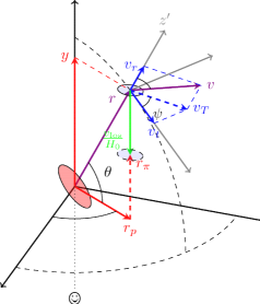
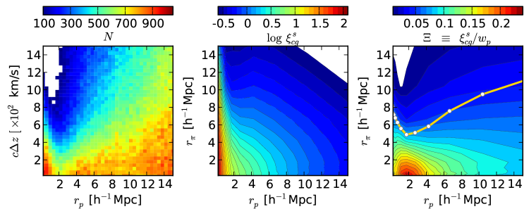
Fig. 1 compares three different ways of illustrating the average distribution of galaxies around clusters in redshift space, using our fiducial cluster mass bin as an example. The left panel simply shows the stacked number counts in cells of equal area on the redshift–$r_{p}$ plane. As mentioned in the introduction, this resembles the traditional way in which the “caustic” curve is identified for individual clusters — we can see an enhancement of the galaxy number distribution at small redshift separations forming the trumpet-shaped pattern. At small $r_{p}$, the galaxy distribution is stretched along the LOS by virial motions, but at $r_{p}\sim 2\,h^{-1}\mathrm{Mpc}$ it is highly compressed along the LOS by infall. While there are strong gradients in $r_{\pi}$ at each $r_{p}$, there is not an obvious line of discontinuity, perhaps because caustics of individual clusters are washed out by scatter in the stack.

Note that although the cells in this representation have equal area, those at large $r_{p}$ have larger volumes in 3-dimensional redshift space because each cell represents a cylindrical ring with radius $r_{p}$ ($V_{\mathrm{cell}}\propto r_{p}^{2}$). The middle panel shows the central quantity in this paper, the redshift–space cluster–galaxy correlation function $\xi^{s}_{cg}$. Since it is equivalent to the overdensity of galaxies around clusters, the dominant feature we see, other than the FOG and Kaiser effects, is the declining trend of overdensity with distance. To highlight the cluster RSD effects at fixed $r_{p}$, in the right panel we plot the contours of $\Xi$, which is defined as the ratio between $\xi^{s}_{cg}(r_{p},r_{\pi})$ and the projected correlation function $w_{p}(r_{p})$ at given $r_{p}$. Since $w_{p}(r_{p})$ is the integral of $\xi^{s}_{cg}$ along $r_{\pi}$ at fixed $r_{p}$, the ratio $\Xi$ has no information that is not already in $\xi^{s}_{cg}$, but by scaling out the radial trend it highlights the RSD effects. The highest peak for $\Xi$ is no longer at the origin (i.e., cluster center), but migrates horizontally to the region around $r_{p}\simeq 2h^{-1}\mathrm{Mpc}$, meaning that the relative distribution of galaxies along $r_{\pi}$ is the most compact at $r_{p}\simeq 2\,h^{-1}\mathrm{Mpc}$ and becomes more spread at both small and large scales. The yellow solid curve in the right panel quantifies this compactness — it shows the characteristic LOS distance $r_{\pi,c}$ at which the amplitude of $\Xi$ drops by $1/e$ from $\Xi(r_{\pi}=0)$ at each $r_{p}$. The curve has a characteristic U-shape, indicating a more compact distribution of galaxies at intermediate projected radii. Note that because $\Xi\propto\xi^{s}_{cg}$ at each $r_{p}$, this U-shaped curve would occupy the same locus in the $\xi^{s}_{cg}$ plot of the middle panel, although we do not show it there.

Figure 3: Joint probability distributions of radial and tangential velocities $P(v_{r},v_{t})$ from the simulation (top panels) and the best–fit using our GIK model (bottom panels), in four different radial bins marked at the bottom of each panel. The colour scales used by panels in the same column are identical, indicated by the colour bar on top.

What determines the location of this characteristic U-shaped curve? It bears some resemblance to the caustic curve for individual clusters, where the fall–off of the galaxy distribution on the redshift–$r_{p}$ diagram is believed to be the natural boundary imposed by the escape velocities at different radii. Indeed, in Fig. 1 the U-shaped curve in the right panel is similar in shape to isodensity contours in the left panel, with the normalization by the mean expected galaxy number removing the somewhat arbitrary geometric weighting ($\propto r_{p}^{2}$) of the straight number–count diagram. However, with no clear discontinuity in $\xi^{s}_{cg}$ or $\Xi$, we cannot relate this curve directly to escape velocities. To explain it quantitatively, we need to understand the average galaxy velocity distribution function around clusters, and in particular, $f(v_{\mathrm{los}}|r_{p},y)$.

Figure 4: Probability distributions of tangential (top panels) and radial velocities (bottom panels) at the same four radial bins as in Fig. 3. In each panel, the gray solid curve shows the 1D marginal distribution. For the left two panels, red dashed and blue dotted curves show the relative contribution from the virialized and infall components, respectively; for the right two top (bottom) panels, blue, green, and red curves show the conditional probability distributions of $v_{t}$ ($v_{r}$) at three different $v_{r}$ ($v_{t}$), as labeled.

For each mass bin of clusters, we stacked all the galaxies in the cluster–centric coordinate to produce a synthetic cluster of that mass bin. Although individual clusters vary in shape and lumpiness, the synthetic clusters are isotropic and smooth by construction. Therefore, in order to fully describe $f(v_{\mathrm{los}}|r_{p},y)$, we only need to measure the joint probability distribution function (PDF) of radial velocity $v_{r}$ and “half” the tangential velocity component $v_{t}$, at each radius $r$, $P(v_{r},v_{t}|r)$, so that

$$f(v_{\mathrm{los}}|r_{p},y)=\int_{-\infty}^{+\infty}P\left(v_{r},v_{t}=\frac{v_{\mathrm{los}}-v_{r}\sin\theta}{\cos\theta}\bigg{|}r\right)\frac{dv_{r}}{\cos\theta},$$ (2)

where $r=\sqrt{r_{p}^{2}+y^{2}}$ and $\theta=\tan^{-1}y/r_{p}$. Here $v_{t}$ represents the tangential velocity ($v_{T}$) component that is projected in the plane of LOS axis and galaxy position vector in the cluster–centric frame (see the 3D diagram in Fig. 2). Given an isotropic cluster, this projected component is $v_{t}=|v_{T}|\cos\psi$ where $\psi$ is randomly distributed between $-90$ and $90$ degrees, hence “half” of $v_{T}$. To avoid redundancy, hereafter we refer to $v_{t}$ simply as the “tangential velocity”. Note that we subtract Hubble flow when defining $v_{r}$, and the probability distribution of $v_{t}$ is symmetric about zero.

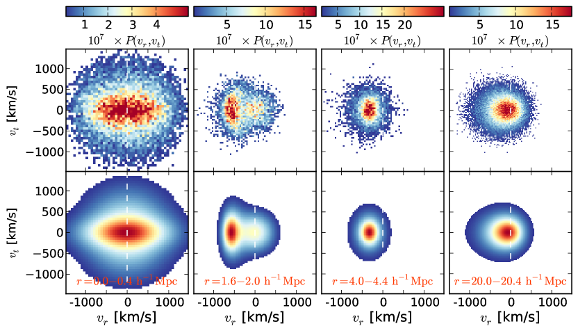
The top panels of Fig. 3 shows the measured $P(v_{r},v_{t})$ for four radial bins that represent four distinctive regimes of GIK around clusters. Starting from the innermost radial bin ($r=0.0\--0.4h^{-1}\mathrm{Mpc}$), the joint velocity distribution appears to be a single component ellipse with the major axis in the radial velocity direction, indicating a preference for radially oriented orbits that may arise from galaxies on first infall or second passage, whose velocity directions have not been randomized (Bertschinger, 1985). Going slightly further out ($r=1.6\--2.0h^{-1}\mathrm{Mpc}$), the joint distribution is clearly resolved into two parts, one virialized Gaussian component with zero means of $v_{r}$ and $v_{t}$, and one radial velocity–dominated component skewed toward negative radial velocities (infall). At $r=4.0\--4.4h^{-1}\mathrm{Mpc}$, near the turn–around radius where infall velocity is comparable to Hubble flow, the virialized component disappears while the infall component has a mean $v_{r}\simeq 400\,\mathrm{kms}^{-1}$ but no skewness. On very large scales ($r=20.0\--20.4h^{-1}\mathrm{Mpc}$), the joint distribution is still largely infall, but skewed toward positive velocities. The joint velocity distribution measured for any of the other radial bins is qualitatively similar to one of the four bins shown here, or some interpolation between two of them. To ensure an accurate description of $f(v_{\mathrm{los}}|r_{p},y)$ at $(r_{p},r_{\pi})<30\,h^{-1}\mathrm{Mpc}$, where the measurements of $\xi^{s}_{cg}$ are most precise, we need to model $P(v_{r},v_{t})$ across all scales from the inner $1\,h^{-1}\mathrm{Mpc}$ to beyond $40\,h^{-1}\mathrm{Mpc}$.

Figure 5: Best–fit GIK (galaxy infall kinematics) model parameters as functions of radius for six mass bins. (a): characteristic infall velocity; (b): fraction of the virialized component; (c): velocity dispersion of the virialized component; (d): radial velocity dispersion of the infall component; (e): tangential velocity dispersion of the infall component; (f): parameter for describing skewness in the radial velocity axis; (g): degrees of freedom for overall kurtosis.

Motivated by the top panels of Fig. 3, we adopt a two–component mixture model for the velocity distribution at any given cluster–centric radius $r$, with the virialized component described by a 2D Gaussian $\mathcal{G}$ and the infall component by a 2D skewed $t$-distribution $\mathcal{T}$:

$$P(v_{r},v_{t})\equiv P(\mathbf{v})=f_{\mathrm{vir}}\cdot\mathcal{G}(\mathbf{v})+(1-f_{\mathrm{vir}})\cdot\mathcal{T}(\mathbf{v}),$$ (3)

where $f_{\mathrm{vir}}\geq 0$ is the fraction of galaxies in the virialized component, approaching zero at large $r$. We refer to the radius beyond which $f_{\mathrm{vir}}=0$ as the “shock radius” $r_{\mathrm{sh}}$, since it marks (at least within the model) the boundary between single–component and two–component flow. By definition $\mathcal{G}$ has zero mean in both radial and tangential axes, and we find it adequate to assume equal dispersions, making $\mathcal{G}$ a function of only one parameter, the virial dispersion $\sigma_{\mathrm{vir}}$ (which is still allowed to vary with $r$). For the infall component, describing the varying degrees of skewness and kurtosis at different $r$ requires a functional form $\mathcal{T}$ with greater complexity. We adopt the skewed $t$–distribution parameterization from Azzalini & Capitanio (2003), with two parameters describing the higher order moments of the velocity distribution ($\alpha$ and $\mathtt{dof}$) in addition to three parameters for the mean and dispersions ($v_{r,c}$, $\sigma_{\mathrm{rad}}$, and $\sigma_{\mathrm{tan}}$). The full expression is

$$\mathcal{T}(\mathbf{v}) = 2\,t_{2}(\mathbf{v};\mathtt{dof})\times$$ (4)

$$T_{1}\left\{\boldsymbol{\alpha}^{T}\boldsymbol{\omega}^{-1}(\mathbf{v}-\mathbf{\bar{v}})\cdot\left(\frac{\mathtt{dof}+2}{Q_{v}+\mathtt{dof}}\right);\mathtt{dof}+2\right\},$$

where $\mathbf{\bar{v}}=\bigl{(}v_{r,c},0\bigl{)}$, $\boldsymbol{\alpha}=\bigl{(}\alpha,0\bigl{)}$, and $\boldsymbol{\omega}=\bigl{(}\sigma_{\mathrm{rad}},\sigma_{\mathrm{tan}}\bigl{)}$ are 2-element vectors, and $Q_{v}=(\mathbf{v}-\mathbf{\bar{v}})^{T}\Sigma^{-1}(\mathbf{v}-\mathbf{\bar{v}})$ is a scalar where

$$\Sigma=\begin{pmatrix}\sigma_{\mathrm{rad}}^{2}&0\\ 0&\sigma_{\mathrm{tan}}^{2}\end{pmatrix}.$$ (5)

For the two rhs terms in Equation 4, $t_{2}$ is the density function of 2D $t$-variate with $\mathtt{dof}$ degrees of freedom,

$$t_{2}(\mathbf{v};\mathtt{dof})=\frac{\Gamma\{(\mathtt{dof}+2)/2\}}{|\Sigma|^{1/2}(\pi\,\mathtt{dof})^{1/2}\Gamma(\mathtt{dof}/2)}\left(1+\frac{Q_{v}}{\mathtt{dof}}\right)^{(\mathtt{dof}+2)/2},$$ (6)

and $T_{1}(x;\mathtt{dof}+2)$ denotes the scalar $t$-distribution function with $\mathtt{dof}+2$ degrees of freedom. Generally speaking, $\boldsymbol{\alpha}$ controls the skewness of $P(v_{r},v_{t})$ in the radial velocity direction, while $\mathtt{dof}$ adjusts the kurtosis in both directions, with lower $\mathtt{dof}$ corresponding to longer non–Gaussian tails. Since $P(v_{r},v_{t})$ is symmetric in the tangential velocity axis, $\boldsymbol{\alpha}$ is reduced to one parameter $\alpha$. $\sigma_{\mathrm{rad}}$ and $\sigma_{\mathrm{tan}}$ describe the dispersion in each direction, and $v_{r,c}$ is the characteristic radial velocity. Therefore, we have seven parameters in total for $P(v_{r},v_{t})$ at every $r$: virialized fraction $f_{\mathrm{vir}}$, velocity dispersion of the virialized component $\sigma_{\mathrm{vir}}$, characteristic infall velocity $v_{r,c}$, two velocity dispersions of the infall component $\sigma_{\mathrm{rad}}$ and $\sigma_{\mathrm{tan}}$, skewness parameter $\alpha$, and kurtosis parameter $\mathtt{dof}$ (effectively reducing to five parameters at $r>r_{\mathrm{sh}}$). With seven parameters, Equation 3 provides an excellent fit for the measured $P(v_{r},v_{t})$ at all scales, as shown visually in the bottom panels of Fig. 3, and in greater detail below. We considered other parameterizations for the infall component, such as sums of Gaussians, but we were unable to find a compact description as accurate as the skewed $t$-distribution, so we obtained poor results in modeling $\xi^{s}_{cg}$.

Figure 6: Functional fits (black curves) to the radial profiles of each GIK parameter measured in simulation (blue circles). Similar to Fig. 5, but only for the fiducial mass bin ($M_{c}=1.259-1.585\times 10^{14}M_{\odot}$). In each panel, the gray shaded area below the radius of maximum infall indicates the regime where cut–offs are required to match the mixing of virial and infall components as shown in the left panel of Fig. 3. Dashed vertical lines indicate the turn–around radius, where the Hubble flow (gray solid line in the top left panel) is equal to the characteristic infall velocity and the skewness parameter $\alpha$ crosses zero in the bottom left panel.

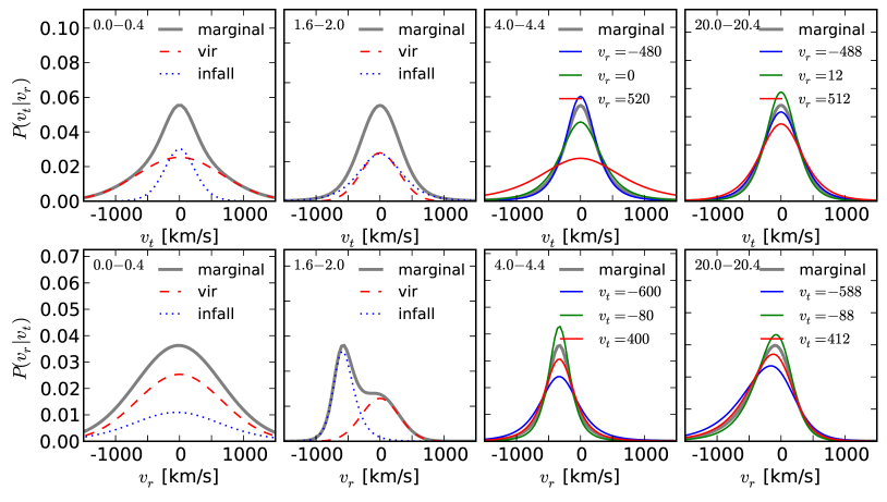
Using the best–fit GIK models, we take a closer look into the properties of $P(v_{r},v_{t})$ at different radii in Fig. 4. In each panel, the gray thick curve shows the 1D marginal probability distribution of tangential ($P(v_{t})$, top) or radial ($P(v_{r})$, bottom) velocities. In the left two columns where $r<r_{\mathrm{sh}}$, the 1D marginal probability distributions of $v_{t}$ (top) and $v_{r}$ (bottom) are decomposed into virialized (red dashed) and infall (blue dotted) components. For the innermost bin, the infall component has a much broader spread in radial velocities than in tangential velocities, signaling its non-virial origin (also see Fig. 3). The second bin shows a more prominent infall component with much smaller radial dispersion in the mixture (bottom). In the right two columns where only infall happens, we show the conditional probability distribution of $v_{t}$ at three fixed values of $v_{r}$ in the top panels, and vice versa in the bottom panels. For the $r=4.0\--4.4\,h^{-1}\mathrm{Mpc}$ bin, as is also apparent in Fig. 3, the conditional distributions show little skewness. However, the conditional probability of $v_{t}$ shows higher kurtosis at more probable values of $v_{r}$. In other words, if we divide the infall population at fixed $r$ into streams of different $v_{r}$, the dominant streams have a more sharply peaked tangential velocity distribution $P(v_{t}|v_{r})$. For instance in the 3rd column, the blue curve in the top panel shows $P(v_{t}|v_{r})$ for the stream of $v_{r}=-480\,\mathrm{kms}^{-1}$, which is near the peak of $P(v_{r})$ according to the bottom panel. Compared to the other two streams of zero (green) and positive radial velocity (red), the blue distribution has many fewer galaxies with $|v_{t}|>500\,\mathrm{kms}^{-1}$. Similarly, the conditional probability of $v_{r}$ also shows higher kurtosis when $v_{t}$ is closer to zero (e.g., green curve in the bottom panel). This kurtosis relation between $v_{t}$ and $v_{r}$ is also apparent in the $r=20.0\--20.4\,h^{-1}\mathrm{Mpc}$ bin, and it is ubiquitous at other distances. In addition, extra skewness in $P(v_{r})$ develops at other distances, and the degree of skewness correlates with $v_{t}$, as seen in the bottom right panel. The skewness switches sign at scales below the turn–around radius, where the radial velocity distributions are negatively skewed (second column, bottom panel, blue dotted curve). The GIK model provides a faithful description of the skewness and kurtosis measured in the simulations, but to avoid clutter, we do not show the simulation measurements in Fig. 4 — the goodness of fit will be ultimately tested in the modeling of $f(v_{\mathrm{los}}|r_{p},y)$.

Figure 7: LOS velocity distribution in nine cells of different projected ($r_{p}$) and LOS ($y$) separations in real space for the fiducial mass bin. Blue histograms and black curves show the measurements from the simulation and the prediction from our best–fit GIK model. The inset panel on top left of each panel indicates the relative position of each cell (red dot) relative to the cluster center (yellow quadrant).

Figure 8: Comparison between the predicted and measured $\xi^{s}_{cg}$ at nine different projected separations for the fiducial mass bin. Blue circles and red triangles with error bars show the simulation measurements with peculiar velocity turned on and off, respectively. Solid curves show the predictions from the best–fit GIK model when peculiar velocity is on, while dashed curves show the direction transformation from $\xi^{r}_{cg}$ to $\xi^{s}_{cg}$ when peculiar velocity is off.

Figure 9: Top panels: Powered exponential fits (solid curves) to the measured (top left) and predicted (top right) profiles of $\xi^{s}_{cg}/w_{p}$ at different $r_{p}$ for the fiducial mass bin. Bottom panels: Best–fit characteristic LOS distance $r_{\pi,c}$ (bottom left) and shape parameter $\beta$ (bottom right) from the top panels; Blue circles and solid curves show the best–fits to simulation measurements and predictions from the GIK model, respectively. The dashed curve in the bottom right panel shows the best–fit $r_{\pi,c}$ for the $\xi^{s}_{cg}$ measured when peculiar velocity is turned off.

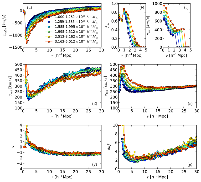
We fit the GIK model with seven parameters to the measurements of $P(v_{r},v_{t})$ at radial bins from $0$ to $40$ $h^{-1}\mathrm{Mpc}$ for six bins of clusters in the simulation. The results are shown in Fig. 5, and we will discuss each panel in turn. The top left panel shows the profiles of the characteristic infall velocity $v_{r,c}$. At given mass, the absolute value of $v_{r,c}$ becomes larger with decreasing distance, peaking at some characteristic radius of maximum infall $r_{\mathrm{mi}}$. Below $r_{\mathrm{mi}}$, as we see in the left column of Fig. 3, the infall component blends into the virialized population, reducing $v_{r,c}$ sharply to zero. The amplitude of $v_{r,c}$ scales with mass as approximately $M^{1/3}$, therefore providing a clear diagnostic of cluster masses. The top middle and right panels show the profiles of virialized fraction $f_{\mathrm{vir}}$ and dispersion of the virial velocities $\sigma_{\mathrm{vir}}$, respectively. The cutoffs below $\sim 1\,h^{-1}\mathrm{Mpc}$ are caused by the same blending effect below $r_{\mathrm{mi}}$, where $f_{\mathrm{vir}}$ stays approximately constant at $0.65$. In this regime, the seperation between the virialized and infall components is no longer sharp (see Fig. 3, left), so while our fit to $P(v_{r},v_{t})$ is accurate, the physical significance of individual parameters is less clear. There are plateaus in the $\sigma_{\mathrm{vir}}$ profiles at $r$$\sim$$2\--4\,h^{-1}\mathrm{Mpc}$ depending on mass, possibly indicating the pre–heating induced by shear flow at the surface where infall and virialized component first contact; however, the virialized component is only $\sim 10\%$ of the total at these radii. The amplitude of $\sigma_{\mathrm{vir}}$ profiles and the extents of both $\sigma_{\mathrm{vir}}$ and $f_{\mathrm{vir}}$ profiles scale with mass. Returning to the infall component, cluster masses affect both the amplitude and shape of the $\sigma_{\mathrm{rad}}$ (middle left) and $\sigma_{\mathrm{tan}}$ (middle right) profiles. More massive clusters induce infall streams with larger (smaller) $\sigma_{\mathrm{rad}}$ on smaller (larger) scales, while $\sigma_{\mathrm{tan}}$ increases monotonically with cluster mass on all scales $r\leq 20\,h^{-1}\mathrm{Mpc}$. Finally, there is little variation of the profiles of $\alpha$ and $\mathtt{dof}$ with mass. The $\alpha$ profiles cross zero at different distances depending on the $v_{r,c}$ profile of each mass bin, but since $\alpha$ decreases slowly with distance at fixed mass, the amplitudes of different curves do not change much. The degrees of freedom start from extremely high values (near–Gaussian tails) at the cluster center, reach a minimum at $\sim 5\,h^{-1}\mathrm{Mpc}$ (a Lorentz distribution has $\mathtt{dof}=1$), then rise up again on large scales. Despite the insensitivity to cluster mass, the systematic variation of $\alpha$ and $\mathtt{dof}$ with radius, not otherwise captured by simple Gaussian or exponential streaming models, is pivotal to the accurate modeling of $f(v_{\mathrm{los}}|r_{p},y)$ and $\xi^{s}_{cg}$ at relevant scales. The interdependence of radial and tangential velocities, seen in Fig. 4, are aslo required for accurate modeling. The cutoffs of $\sigma_{\mathrm{tan}}$ and $\alpha$ profiles on small scales have the same blending origin as those of $v_{r,c}$ and $f_{\mathrm{vir}}$.

Figure 10: Effects of perturbing each GIK component on the characteristic U-shaped curve of $\xi^{s}_{cg}$. In each row, the amplitude of one of the components (from top to bottom: fraction and velocity dispersion of the virialized component $f_{vir}$ and $\sigma_{vir}$ , radial velocity profile $v_{rad}$, radial velocity dispersion $\sigma_{rad}$, and tangential velocity dispersion $\sigma_{tan}$) is changed from its fiducial value by $\pm 50\%$, and we fit powered exponential functions to the predicted $\xi^{s}_{cg}$ at each $r_{p}$. The right panels show the impact of these changes on the $r_{\pi,c}(r_{p})$ curves, comparing the predictions of the modified model (blue and red) to the fiducial model (black).

To summarize, Fig. 5 shows that higher mass clusters have, as expected, higher amplitude characteristic infall curves $v_{r,c}$, virialized components with higher velocity dispersion $\sigma_{\mathrm{vir}}$ that extend to large radii $r_{\mathrm{sh}}$, and higher tangential velocity dispersions $\sigma_{\mathrm{tan}}$ within the infall component. The radial dispersion $\sigma_{\mathrm{rad}}$ has weaker mass dependence that reverses sign at $r$$\sim$$5\,h^{-1}\mathrm{Mpc}$, and the profiles of $\alpha(r)$ and $\mathtt{dof}(r)$, which control the shape of the distribution function of the infall component, show nearly universal, mass–independent bahavior. We are especially interested in extracting the characteristic infall curves $v_{r,c}(r)$, as these probe the extended mass profile around clusters and should be insensitive to physics that may alter the dispersions of satellite galaxies within halos. The smooth behaviour and systematic trends in Fig. 5 suggest that isolating $v_{r,c}$ will be feasible, and the profiles of $\sigma_{\mathrm{vir}}(r)$ and $\sigma_{\mathrm{tan}}(r)$ offer additional mass diagnostics. The main area of uncertainty is the cutoff behaviour below the maximum infall radius $r_{\mathrm{mi}}\approx 1\,h^{-1}\mathrm{Mpc}$. This should have little impact in practical applications, as shot noise and “fiber collision” effects (Blanton et al., 2003) make $\xi^{s}_{cg}$ difficult to measure at small $r_{p}$, and $\xi^{s}_{cg}$ at a given $r_{p}$ is absolutely unaffected by any scales $r<r_{p}$.

Figure 11: Constraints on each component of the GIK model from the simulation measurements of $\xi^{s}_{cg}$. Yellow and gray contours indicate the $68\%$ and $95\%$ confidence regions. The blue star in the top left panel and dashed curves in the remaining panels show the direct measurements from the simulation.

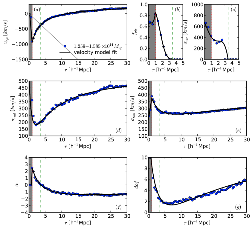
To describe the variations of these seven parameters with $r$, we fit them with analytic functions chosen to match the numerically measured shapes. We fit $v_{r,c}(r)$ with a 3-parameter function,

$$v_{r,c}(r)=q_{1}-\frac{p_{1}}{(r+r_{\mathrm{mi}})^{\beta_{1}}},$$ (7)

where $r_{\mathrm{mi}}$ is the maximum infall radius beyond which $v_{r,c}$ is exponentially cut off to zero, $q_{1}$ controls the maximum amplitude, and $p_{1}$ and $\beta_{1}$ together control the asymptote and slope of the large scale power–law behaviour, respectively. The virialized fractions are well described by a “powered exponential”,

$$f_{\mathrm{vir}}(r)=\exp\left\{-\left(\frac{r}{r_{0}}\right)^{3}\right\},$$ (8)

where $r_{0}$ is a characteristic radius of the cluster. We set the radius at which $f_{\mathrm{vir}}(r)$ falls to $0.3\%$ as the shock radius $r_{\mathrm{sh}}$, which corresponds to $1.8\,r_{0}$, and we set $f_{\mathrm{vir}}(r>r_{\mathrm{sh}})=0$. The velocity dispersion profiles of the virialized component can be described by

$$\sigma_{\mathrm{vir}}(r)=\sigma_{0}\left\{1+\left(1-\frac{r}{r_{*}}\right)^{\nu}\right\}^{3},$$ (9)

where we find $\nu=1.315$ provides a good fit to all the mass bins, and we impose the constraint that the plateau happens at $r=r_{\mathrm{sh}}$, so that $r_{*}$ is determined by the best–fit $r_{\mathrm{sh}}$ from $f_{\mathrm{vir}}$ via $r_{*}\equiv 2^{-1/\nu}r_{\mathrm{sh}}=0.59\,r_{\mathrm{sh}}$. The remaining four nuisance profiles are well described by one generic function,

$$\left\{\sigma_{\mathrm{rad}},\,\sigma_{\mathrm{tan}},\,\alpha,\,\mathtt{dof}\right\}(r)=q_{i}-p_{i}\frac{r}{(r+r_{i})^{\beta_{i}}},\quad\mbox{$i\in\{2,3,4,5\}$},$$ (10)

where the effects of $q_{i}$, $p_{i}$, and $\beta_{i}$ are similar to that of $q_{0}$, $p_{0}$, and $\beta_{0}$ in Equation 7, except that the minima happen at $r_{i}/(\beta_{i}-1)$ instead of $r_{i}$.

The best–fit functions are shown in Fig. 6 for the fiducial mass bin. The gray shaded area in each panel indicates the $r<r_{\mathrm{mi}}$ regime, where we apply simple cut–offs (exponential or polynomial) to mimic the rough measurements from simulation. We emphasize again that the cut–offs do not affect the modeling of $f(v_{\mathrm{los}}|r_{p},y)$ and $\xi^{s}_{cg}$ at $r_{p}>r_{\mathrm{mi}}$. The gray line in the top left panel indicates the amplitude of Hubble flow, crossing $v_{r,c}(r)$ at the turn–around radius, which is indicated in each panel by the vertical dashed line.

3 Modeling of $\mathbf{\xi^{s}_{cg}}$

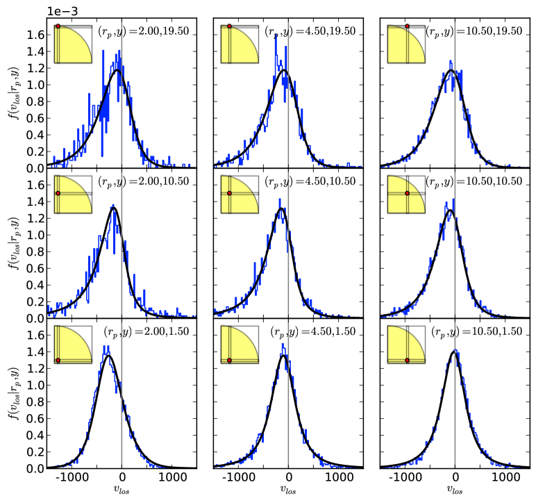
The GIK model describes average galaxy motions around clusters in 3D, but the modeling of $\xi^{s}_{cg}$ requires predicting the 1D galaxy motions projected along the LOS at any given ($r_{p},y$). Fig. 7 compares the LOS velocity distribution $f(v_{\mathrm{los}}|r_{p},y)$ measured directly from the simulation to that predicted from the best–fit GIK model (i.e., using the functional fits shown in Fig. 6), at nine different cells around clusters in the fiducial mass bin. The relative position of each cell around the cluster center is indicated by the red dot in the inset quadrant. Although the GIK model is calibrated using the same simulation that $f(v_{\mathrm{los}}|r_{p},y)$ is measured from, the agreement we see in Fig. 7 in all panels is highly non–trivial — the 2D mixture model accurately recovers the varying degrees of skewness and kurtosis of LOS velocity distributions at different positions of $(r_{p},y)$, whereas a less comprehensive model (e.g., only fitting to the first and second moments, or treating tangential and radial velocities independently) would fail. The agreement in Fig. 7 also reconfirms that our best–fit GIK model provides an excellent description of the galaxy kinematics in the Millennium simulation.

Once we predict $f(v_{\mathrm{los}}|r_{p},y)$, it is straightforward to predict $\xi^{s}_{cg}$ by convolving $f(v_{\mathrm{los}}|r_{p},y)$ with the real–space cluster–galaxy correlation function $\xi^{r}_{cg}$, then compare to the $\xi^{s}_{cg}$ measured directly from simulation. The convolution is, expressed in a form more explicit than Equation 1,

$$\xi^{s}_{cg}(r_{p},r_{\pi})+1 = H_{0}\int_{-\infty}^{+\infty}\left[\xi^{r}_{cg}\big{(}\sqrt{r_{p}^{2}+y^{2}}\big{)}+1\right]\times$$ (11)

$$f\big{(}H_{0}(r_{\pi}-y)|r_{p},y\big{)}dy.$$

To make sure that the $\xi^{s}_{cg}$ comparison is unaffected by any inaccuracies in $\xi^{r}_{cg}$, we use the $\xi^{r}_{cg}$ directly measured from simulation to convolve with $f(v_{\mathrm{los}}|r_{p},y)$. For measuring $\xi^{r}_{cg}$, we count the numbers of galaxies around clusters in spherical shells of successive radii, ranging from $10\,h^{-1}\mathrm{kpc}$ to $50\,h^{-1}\mathrm{Mpc}$ with logarithmic intervals, average over all clusters in each bin, and normalize by the galaxy numbers expected in a randomly located shell of equal volume. We measure $\xi^{s}_{cg}$ in a similar way, counting galaxies in cylindrical rings of successive $r_{\pi}$ for each $r_{p}$ (assuming a distant–observer approximation so that the LOS is an axis of the box).

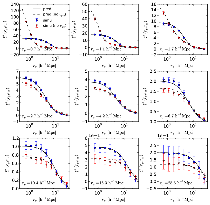
Fig. 8 compares the $\xi^{s}_{cg}$ from convolution to the simulation measurements for the fiducial mass bin from $r_{p}=0.7\,h^{-1}\mathrm{Mpc}$ to $25.5\,h^{-1}\mathrm{Mpc}$ ($r_{p}$ increasing from top to bottom, left to right). In each panel, blue circles with errorbars are the $\xi^{s}_{cg}$ measured directly from the simulation, while the solid curves are predictions from the best–fit GIK model using Equation 11; red triangles with errorbars are the $\xi^{s}_{cg}$ measured when the peculiar velocity of each object is set to zero in the simulation, i.e., setting $\xi^{s}_{cg}(r_{p},r_{\pi})\equiv\xi^{r}_{cg}\left(\sqrt{r_{p}^{2}+r_{\pi}^{2}}\right)$. There is overall good agreement between $\xi^{s}_{cg}$ predicted from the best–fit GIK model and measured from simulation, except for the $r_{p}=4.2\,h^{-1}\mathrm{Mpc}$ and $6.7\,h^{-1}\mathrm{Mpc}$ panels where the model predictions are slightly higher than the measurements at small $r_{\pi}$. The minor discrepancy probably comes from the stochastic noise in measurements along one particular sight line (similar to cosmic variance), as there is already discrepancy for the no–$v_{\mathrm{pec}}$ cases (red triangles vs. dashed curves) in the same two panels before convolving with $f(v_{\mathrm{los}}|r_{p},y)$ — the redshift space correlations are measured along the $z$–axis of simulation box, while the real space correlation is measured assuming isotropy of the entire box.

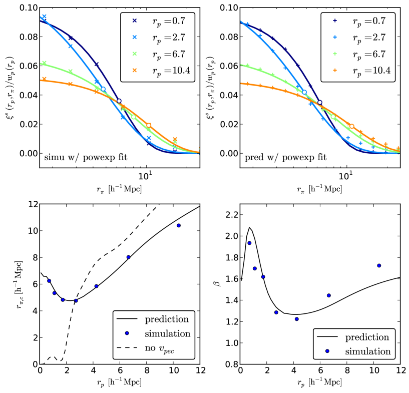
By comparing the two cases ($v_{\mathrm{pec}}$ vs. no–$v_{\mathrm{pec}}$) within each panel, Fig. 8 also nicely illustrates the two major RSD effects — $\xi^{s}_{cg}$ along the LOS is suppressed by random dispersion for small $r_{p}$, but is amplified by galaxy infall for large $r_{p}$. To further quantify these deformations, we fit a powered exponential function to the $\xi^{s}_{cg}$ at each $r_{p}$, which is equivalent to fitting a normalized powered exponential function to $\Xi$

$$\Xi(r_{\pi}|r_{p})\equiv\frac{\xi^{s}_{cg}(r_{p},r_{\pi})}{w_{p}(r_{p})}\bigg{|}_{r_{p}}\sim\exp\left\{-\left|\frac{r_{\pi}}{r_{\pi,c}}\right|^{\beta}\right\},$$ (12)

where $r_{\pi,c}$ is the characteristic length scale at which $\xi^{s}_{cg}$ drops to $1/e$ of its maximum value at $r_{\pi}=0$. The shape parameter $\beta$ yields a Gaussian cutoff for $\beta=2$ and simple exponential for $\beta=1$, though any value is allowed in the fit.

Fig. 9 summarizes the fits of $\Xi$ measured from simulation (crosses in the top left panel) and predicted by the best–fit GIK model (plus symbols in the top right panel) at four different $r_{p}$. The fits (solid curves) in the two panels are very similar, so we focus on the top left panel here. The open circle through each curve indicates the position of $r_{\pi,c}$, which migrates from $\sim 6.5\,h^{-1}\mathrm{Mpc}$ at $r_{p}=0.7\,h^{-1}\mathrm{Mpc}$ inward to $\sim 5.0\,h^{-1}\mathrm{Mpc}$ at $r_{p}=2.7\,h^{-1}\mathrm{Mpc}$, and then outward to $\sim 8$ and $10\,h^{-1}\mathrm{Mpc}$ at $r_{p}=6.7$ and $10.4\,h^{-1}\mathrm{Mpc}$, respectively. This “precession” of $r_{\pi,c}(r_{p})$ is more clearly shown in the bottom left panel, where the blue circles and solid curves plot the migration of $r_{\pi,c}$ as function of $r_{p}$ from fits to the measurements and model predictions, respectively. This characteristic U-shaped curve is the same one shown in the right panel of Fig. 1. Also shown in the bottom left panel is $r_{\pi,c}(r_{p})$ for the no–$v_{\mathrm{pec}}$ case, which grows monotonically with increasing $r_{p}$. This can be easily understood for a power–law $\xi^{r}_{cg}\propto r^{-\gamma}$, where $\xi^{s}_{cg}(r_{p},r_{\pi})\propto(1+(r_{\pi}/r_{p})^{2})^{-\gamma/2}$ with no $v_{\mathrm{pec}}$, hence $r_{\pi,c}\propto r_{p}$. The change of slope around $r_{p}\simeq 2.5\,h^{-1}\mathrm{Mpc}$ for the no–$v_{\mathrm{pec}}$ case is caused by the change of $\gamma$ during transition from the 1-halo to 2-halo regime. The bottom right panel shows the corresponding changes of $\beta$ as function of $r_{p}$, which largely follow (in a slightly lagged fashion) the variations in $r_{\pi,c}(r_{p})$, and which are again well described by the GIK model. We will focus on $r_{\pi,c}(r_{p})$ as the representative feature of $\xi^{s}_{cg}$ in the next section.

Note that the powered–exponential is not intended to be a viable model of $\Xi$, just a compact and visually appealing way of quantifying the characteristics of $\Xi$. Therefore, although the powered–exponentials do not fit well on scales larger than $\sim 15\,h^{-1}\mathrm{Mpc}$, the best–fit $r_{\pi,c}$ and $\beta$ still effectively capture the main features of each curve.

4 Bayesian Inference of Velocity Distribution

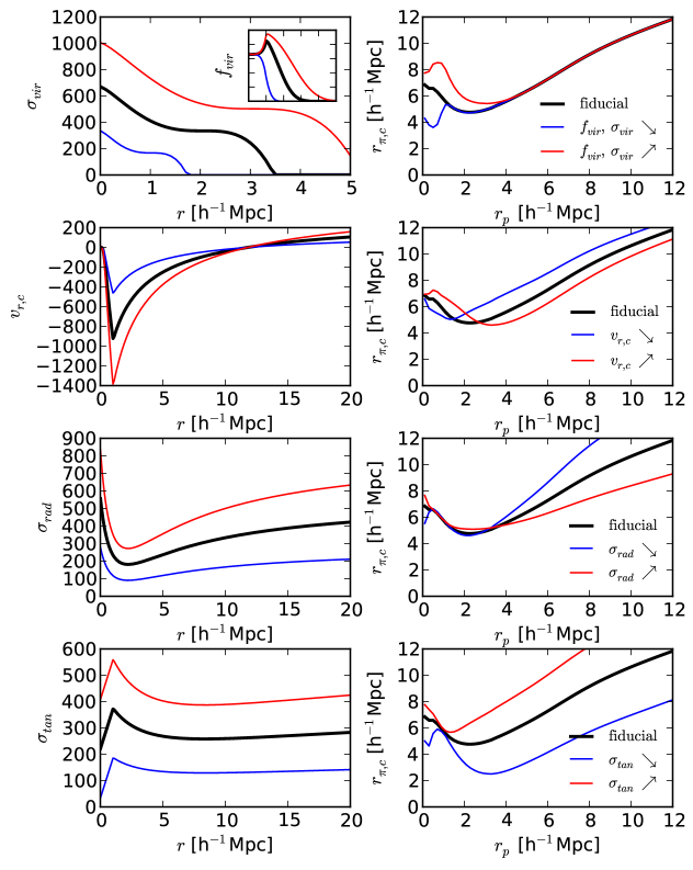
Armed with an accurate GIK model that correctly predicts the $\xi^{s}_{cg}$ signal, we are in the position to investigate the origin of the “U-shaped curve” of Fig. 1, and, more importantly, to examine the intrinsic degeneracies within the modeling of $\xi^{s}_{cg}$, which carries valuable information that we hope to exploit robustly. To achieve this understanding, we perturb the elements of the velocity field one at a time, changing the amplitude of a single model component by $\pm 50\%$ while holding others fixed. In §2 we found that among the seven parameters in the GIK model (see Fig. 5), $\alpha$ and $\mathtt{dof}$ are insensitive to cluster mass, so we focus on the remaining five parameters, linking $\sigma_{\mathrm{vir}}$ and $f_{\mathrm{vir}}$ so that there are four independent GIK components. Each row in Fig. 10 shows the results of perturbing the amplitude of one component: properties of the virialized population $\sigma_{\mathrm{vir}}$+$f_{\mathrm{vir}}$, characteristic infall velocity $v_{r,c}$, radial velocity dispersion of the infall population $\sigma_{\mathrm{rad}}$, or tangential velocity dispersion of the infall population $\sigma_{\mathrm{tan}}$. For the first row, we change the amplitude of $\sigma_{\mathrm{vir}}$ by changing the value of $\sigma_{0}$ in Equation 9, and we simultaneously change the value of $r_{\mathrm{sh}}$ proportionally with $\sigma_{0}$, which in turn expands $f_{\mathrm{vir}}$ along the $r$ axis (the inset axis). For the rest, since they all have similar parameterization, we change the amplitudes via multiplying $p_{i}$ and $q_{i}$ in Equation 7 and 10 by the same factor. We will describe each row in turn, from top to bottom.

• When $\sigma_{\mathrm{vir}}$ is increased and $f_{\mathrm{vir}}$ is expanded, the virialized region becomes hotter and larger, producing more flattened $\xi^{s}_{cg}$ for $r_{p}<r_{\mathrm{sh}}$ while having no effect for $r_{p}\geq r_{\mathrm{sh}}$. This is the portion of the FOG effect caused by virialized dispersion.

• When the infall velocity $v_{r,c}$ is faster (more negative), galaxies at large $r_{p}$ are shifted closer to the cluster center (more “Kaiser compression”), therefore reducing $r_{\pi,c}$. However, at small $r_{p}$ the infall is strong enough to send galaxies from one side of the cluster in real space ($y<0$ or $y>0$) to the opposite side in redshift space ($r_{\pi}>0$ or $r_{\pi}<0$). This is the portion of the FOG effect caused by infall. The characteristic projected separation $r_{p}^{*}$ at which the U-shaped curve reaches a minimum is then set by the transition from large–scale compression to small–scale inversion, shifting to a larger scale when infall becomes stronger. The value of $r_{\pi,c}$ at the minimum also decreases slightly as $v_{r,c}$ increases.

• When $\sigma_{\mathrm{rad}}$ is higher, the velocity ellipses of $P(v_{r},v_{t})$ are more elongated along the radial velocity axis. Since the ellipses sit mostly at the negative half of the radial velocity axis, higher $\sigma_{\mathrm{rad}}$ effectively leads to overall stronger infall. However, at smaller LOS distance ($y<r_{p}$), the LOS velocity distribution is insensitive to the changes in $\sigma_{\mathrm{rad}}$ ($\theta<\pi/4$ in Equation 2), so the stronger infall only starts to affect $r_{\pi,c}$ at large scales where $r_{\pi,c}$ is comparable to $r_{p}$, and the impact on $r_{\pi,c}$ increases as a function of $r_{p}$.

• When $\sigma_{\mathrm{tan}}$ is higher, the velocity ellipses of $P(v_{r},v_{t})$ are more stretched along the tangential velocity axis, effectively increasing the dispersions of $v_{\mathrm{los}}$ without modifying the mean. Therefore, similar to the effect of $\sigma_{\mathrm{vir}}$ on small scales, higher $\sigma_{\mathrm{tan}}$ increases $r_{\pi,c}$ on all scales, though the fractional impact is largest at $r_{\pi}\gtrsim r_{\mathrm{sh}}$.

The basic U-shape of the $r_{\pi,c}$ vs. $r_{p}$ curve is straightforward to understand: FOG stretching at small $r_{p}$ gives way to Kaiser compression at intermediate $r_{p}$ which gives way to Hubble flow expansion at large $r_{p}$. However, Fig. 10 shows that the detailed shape of this curve, and more generally of $\xi^{s}_{cg}(r_{p},r_{\pi})$, reflects a complex interplay among the four components of the galaxy kinematics around clusters.

Figure 12: Measurements of $\xi^{s}_{cg}$ for SDSS groups in three bins of BCG stellar mass. The yellow U-shaped curve in each panel shows the characteristic LOS distance $r_{\pi,c}$ at each projected separation $r_{p}$. The contour scales are the same for all panels, indicated by the colour bars on top.

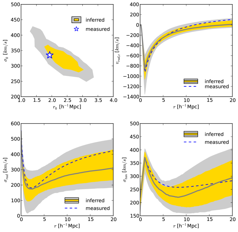
Crucially, the impact of each GIK component has a distinct scale and amplitude dependence, suggesting that they can be inferred from $\xi^{s}_{cg}$ measurements with only limited degeneracy. To confirm this expectation, we construct a Gaussian likelihood model with the measurements of $\xi^{s}_{cg}$ in Fig. 8 as the input data, and the functional parameters introduced in §2 as our model parameters. The parameters we vary in the model are, $\{q_{1}$, $p_{1}$, $\beta_{1}\}$ for the characteristic infall velocity (Equation 7), $\{r_{0}$, $\sigma_{0}\}$ for the virialized component (Equations 9 and 8), $\{q_{2}$, $p_{2}$, $r_{2}$, $\beta_{2}\}$ for the radial velocity dispersion (Equation 10), and $\{q_{3}$, $p_{3}$, $r_{3}$, $\beta_{3}\}$ for the tangential velocity dispersion (Equation 10). In this way, we allow maximum freedom for the shape and amplitude of each component to vary during the fit. We keep the remaining parameters fixed to their best–fit values in Fig. 6, as they appear to be insensitive to cluster masses (see Fig. 5) — we keep the radial profiles of $\alpha$ and $\mathtt{dof}$ fixed in amplitude and shape, and we maintain the shapes of the $\sigma_{\mathrm{vir}}$ and $f_{\mathrm{vir}}$ profiles, while allowing them to change scale along both axes via $r_{0}$ and $\sigma_{0}$. The Gaussian log–likelihood is thus

$$\ln\mathcal{L}(\xi^{s}_{cg}|\boldsymbol{\theta})\propto-\frac{1}{2}\left(\xi^{s}_{cg}-\xi^{s}_{cg}(\boldsymbol{\theta})\right)^{T}C^{-1}\left(\xi^{s}_{cg}-\xi^{s}_{cg}(\boldsymbol{\theta})\right),$$ (13)

where

$$\boldsymbol{\theta}\equiv\{q_{1},p_{1},\beta_{1},r_{0},\sigma_{0},q_{2},p_{2},r_{2},\beta_{2},q_{3},p_{3},r_{3},\beta_{3}\},$$ (14)

and $C$ is the data covariance matrix measured from Jackknife re–sampling of the simulation volume. For demonstration purposes, we use the direct simulation measurements of $\xi^{r}_{cg}$ to convolve with the predicted $f(v_{\mathrm{los}}|r_{p},y)$. When applying the model to observations, $\xi^{r}_{cg}$ should either be inverted from the measured $w_{p}$ (see §5) or directly predicted from theoretical models (papers II and III).

We adopt a Bayesian approach, assuming uninformative priors for all the parameters that are allowed to vary. For the parameter inference, we sample the posterior distributions using a Markov Chain Monte Carlo (MCMC), where an adaptive Metropolis step method is utilized during the burn–in period. The whole chain has 15,000 iterations, 5,000 of which belong to the burn–in period, where auto–correlation tests show good convergence before actual sampling. We emphasize that while we used the $r_{\pi,c}(r_{p})$ curve for illustration in Fig. 10, our statistical inference of GIK uses the full $\xi^{s}_{cg}(r_{p},r_{\pi})$, as indicated by Equation 13.

Fig. 11 presents the constraints on the four GIK components inferred from the MCMC when we apply this fitting procedure to the $\xi^{s}_{cg}$ measurements from the fiducial mass bin. Yellow and gray contours show the $68\%$ and $95\%$ confidence limits, respectively. For the constraints on $v_{r,c}$, $\sigma_{\mathrm{rad}}$, and $\sigma_{\mathrm{tan}}$ profiles, we compute the median (68% and 95%) curves discretely at each $r$ as the median (68% and 95%) functional values calculated from all the iterations at that $r$, rather than the functional values calculated from the median (68% and 95%) parameters. The blue star in the top left panel and blue dashed curves in the other panels indicate the direct fits to simulation measurements of GIK in Fig. 6. The constraints derived from $\xi^{s}_{cg}$ show overall agreement with the direct fits, confirming that the distinctive effect of each GIK component allows us to constrain the overall model with minimal ambiguity. In particular, the characteristic radial infall curve $v_{r,c}(r)$ is inferred with small uncertainty from this cluster sample ($N_{\mathrm{cluster}}=691$) . The medians are slightly offset from the fiducial values, possibly because of the same stochastic noise that causes the discrepancies in Fig. 8, but the offsets are smaller than the $68\%$ statistical uncertainty.

5 Application to SDSS Groups

We defer a comprehensive calibration and application of the GIK model to the future, but as a proof of concept, we apply the current GIK model to $\xi^{s}_{cg}$ measured for rich galaxy groups found in the SDSS. We employ the group catalog of Yang et al. (2007) in the local universe ($z<0.2$) found in the spectroscopic data of SDSS Data Release 7 (DR7; Abazajian et al., 2009). Each group was identified initially with a friends-of-friends scheme in the redshift space and kept in the catalog by an iterative adaptive filter method. For more details on the construction of the catalog, we refer the reader to Yang et al. (2007). Small groups are likely to suffer more contamination and to have weaker infall patterns. We therefore select $6691$ groups that have relatively high stellar mass ($\log M_{*}/M_{\odot}\geq 11.0$) in their brightest cluster galaxies (BCGs) and have at least three identified galaxy members; We describe these groups as our “cluster” sample. We divide the $6691$ clusters further into three BCG stellar mass bins, with $\log M_{*}=11.00\--11.20$ ($N_{c}=4018$), $\log M_{*}=11.20\--11.40$ ($N_{c}=2027$), and $\log M_{*}=11.40\--11.90$ ($N_{c}=646$), respectively. For the first–cut analysis here, we will use the positions of BCGs as the cluster centers, without modeling the mis–centering effect (Skibba et al., 2011). For the galaxy sample, we use the dr72safe0 sample within the NYU Value-Added Galaxy Catalog (Blanton et al., 2005) derived from the main spectroscopic sample in DR7, containing $N_{g}=534206$ galaxies with K+E–corrected $r$-band magnitudes between $-24$ and $-16$ at $z<0.2$.

In contrast to the simulation where the expected number of cluster–random galaxy pairs is known precisely, we have to construct random catalogs of galaxy samples that have the same angular and redshift selection functions as the observed galaxy sample. We generate the angular completeness map in the format of non–overlapping polygons from the dr72safe0 window function using MANGLE (Swanson et al., 2008), then draw $N_{g}$ random galaxy coordinates from each polygon based on its spectroscopic completeness. To account for the redshift selection function, we randomly shuffle the redshifts of observed galaxies and assign them to the random coordinates. This shuffling procedure is equivalent to drawing redshifts from the parent redshift distribution of the observed sample when $N_{g}$ is large. To reduce the random noise, we repeat the process for ten times and construct a random galaxy sample with $N_{r}=10\times N_{g}$.

We measure $\xi^{s}_{cg}$ using the Davis & Peebles (1983) estimator,

$$\xi^{s}_{cg}(r_{p},r_{\pi})=\frac{N_{r}}{N_{g}}\frac{N_{CG}(rp,r_{\pi})}{N_{CR}(rp,r_{\pi})}-1,$$ (15)

where $N_{CG}$ and $N_{CR}$ are the cluster–galaxy pairs and cluster–random galaxy pairs, respectively. We estimate measurement uncertainties on $\xi^{s}_{cg}$ using the Jackknife re–sampling method. In addition, we also measure the projected cluster–galaxy correlations $w_{p}$ from the same data and random galaxy samples using an integration length of $r_{\pi}^{\mathrm{max}}=40\,h^{-1}\mathrm{Mpc}$.

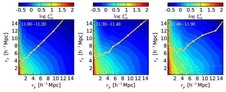
Fig. 12 shows the $\xi^{s}_{cg}$ measured for the three bins of clusters and the characteristic U-shaped curves derived from $\xi^{s}_{cg}$. The colour scales are the same in all panels, so it is clear that clusters in higher stellar mass bins have on average higher masses, showing stronger correlation signals at fixed ($r_{p},r_{\pi}$). The BCG stellar mass, however, is only a loose indicator of total cluster mass. To completely model $\xi^{s}_{cg}$ measured in bins of BCG stellar mass, we should predict $\xi^{r}_{cg}$ and $f(v_{\mathrm{los}}|r_{p},y)$ as functions of $M$ to get $\xi^{s}_{cg}(M)$, then convolve $\xi^{s}_{cg}(M)$ with scatter in the $M_{*}$–$M$ relation weighted by the cluster mass function $dn/dM$. This type of comprehensive model has been used to interpret weak lensing measurements (Sheldon et al., 2009) for SDSS MaxBCG clusters by Rozo et al. (2010), Tinker et al. (2012), and Zu et al. (2012), and we will adopt it for $\xi^{s}_{cg}$ modeling in future work. For our first–cut analysis here, we will infer average GIK properties of the Yang et al. (2007) groups by treating each $M_{*}$-bin as though it were a single halo mass bin.

Figure 13: Projected correlations $w_{p}$ (left), 3D real space correlations $\xi^{r}_{cg}$ (middle), and characteristic U-shaped curves (right) for SDSS groups of different BCG stellar mass. Left: Circles with error bars show the measurements of $w_{p}$ from SDSS and solid curves are the best–fit models. Middle: Solid curves show the $\xi^{r}_{cg}$ inverted from best–fit $w_{p}$ in the left panel. Dashed and dotted curves show the contributions from the 1-h and 2-h terms in the model. Right: Same as the yellow curves shown in Fig. 12.

Figure 14: Similar to Fig. 11, but for the $\xi^{s}_{cg}$ measurements from SDSS groups with BCG $\log\,M_{*}/M_{\odot}=11.2-11.4$ (green contours) and $11.4-11.9$ (red contours). The dashed curve in the top right panel shows the characteristic infall velocity of clusters in mass bin $1.0\--1.259\times 10^{14}\,h^{-1}M_{\odot}$, measured from the Millennium simulation.

Figure 15: Comparison between the predicted and measured $\xi^{s}_{cg}$ at ten different projected separations for SDSS groups. Green circles and red triangles with error bars show the measurements for the two BCG stellar mass bins (marked in the top left panel), respectively. Solid curves show the predictions from the best–fit GIK model.

The first step is to reconstruct $\xi^{r}_{cg}$ from the measurements of $w_{p}$. We adopt the $\xi^{r}_{cg}$ prescription from Zu et al. (2012). This prescription, similar to that of Hayashi & White (2008), sets the value of $\xi^{r}_{cg}$ at each $r$ as the maximum of a Navarro–Frenk–White profile (Navarro et al., 1996, 1997, NFW) and a biased non–linear matter correlation function. We refer to these two components as “1-h” (for one–halo) and “2-h” (for two–halo), respectively. To ensure a reasonable behaviour of $\xi^{r}_{cg}$ on large scales, we fix the non–linear matter correlation to be that from a flat $\Lambda$CDM $(\Omega_{m}=0.23,\sigma_{8}=0.79)$ universe at $z=0.1$, computed from the HALOFIT model (Smith et al., 2003). Therefore, the $\xi^{r}_{cg}$ model has three parameters, including cluster bias, scale radius, and normalization of the NFW profile. For more details about the modeling and calibration of $\xi^{r}_{cg}$, we refer the readers to Zu et al. (2012). We compute $w_{p}$ by integrating $\xi^{r}_{cg}$ using the same $r_{\pi}^{\mathrm{max}}=40\,h^{-1}\mathrm{Mpc}$ and fit it to the measured $w_{p}$ for each cluster bin. As pointed out by Croft et al. (1999) and Li et al. (2012), although this reconstruction does not necessarily recover the correct 1-h and 2-h terms, it provides a reasonable estimate of the underlying $\xi^{r}_{cg}$.

Fig. 13 shows the results of this reconstruction. The left panel compares the measured $w_{p}$ to the best–fits using the 3–parameter model, showing good agreement for the two highest stellar mass bins, with some discrepancies on large scales for the lowest bin. These discrepancies may be caused by deficiency of our simplified $w_{p}$ model, or by contamination from interlopers in the group catalog. To avoid further complications, we drop the lowest bin from our following analysis. The middle panel shows the best–fit $\xi^{r}_{cg}$ for each bin, and the corresponding 1-h and 2-h terms. The curves for the two higher stellar mass bins will be the input $\xi^{r}_{cg}$ for our Bayesian inferences below. In the right panel, we put together the three U-shaped curves shown individually in Fig. 12. They are qualitatively similar to the curves we see in simulation, and the variation with BCG stellar mass is as expected — higher mass bins have stronger infall and larger dispersion of virial motions, thus smaller $r_{\pi,c}$ on large scales but larger $r_{\pi,c}$ on small scales.

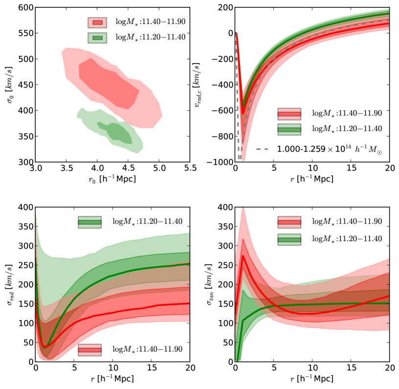
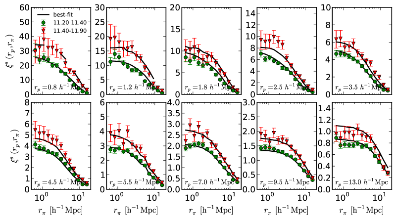
Given the best–fit $\xi^{r}_{cg}$ reconstructed from $w_{p}$, we apply the same Bayesian inference described in §4 to the measurements of $\xi^{s}_{cg}(r_{p},r_{\pi})$ for each of the two higher stellar mass bins of SDSS clusters. We vary the same set of parameters listed in Equation 14. All the input data points of $\xi^{s}_{cg}$ are shown in Fig. 15 (discussed further below) as red triangles and blue circles with error bars. Fig. 14 presents the constraints on the average GIK for the two bins. The overall results are remarkably similar to what we see in the simulation (compare to Fig. 11), but with some anomalies that likely arise from observational uncertainties. In particular, the two inferred values of $r_{0}$ (radius at which $f_{\mathrm{vir}}=1/e$) are considerably larger than expected for clusters with $M\sim 10^{14}\,h^{-1}M_{\odot}$ (e.g., $r_{0}<3h^{-1}\mathrm{Mpc}$ for all the mass bins in Fig. 5). This difference is likely caused by a combination of mis–centering, contamination, and scatter between BCG stellar mass and cluster mass, all of which blur the $\xi^{s}_{cg}$ measurements on small scales, mimicking a much stronger virial component. However, even though we do not model these systematic effects, we find trends of each GIK component with stellar mass that track the trends with cluster mass seen in the simulation (Fig. 5). In particular, the high stellar mass bin has a higher amplitude of virial dispersion $\sigma_{0}$, stronger infall $v_{r,c}$, smaller dispersion in radial velocities $\sigma_{\mathrm{rad}}$, and higher (comparable) dispersion in tangential velocities $\sigma_{\mathrm{tan}}$ on small (large) scales. The dashed curve in the upper right panel of Fig. 14 repeats the black points in Fig. 5a, marking the infall curve $v_{r,c}(r)$ measured for $1.0\--1.259\times 10^{14}\,h^{-1}M_{\odot}$ halos in the Millennium simulation. The agreement with our SDSS measurement for the higher stellar mass bin is very good, indicating that the mass scale of these BCG $\log\,M_{*}/M_{\odot}=11.4\--11.9$ groups is about $10^{14}\,h^{-1}M_{\odot}$, while that of the $\log\,M_{*}/M_{\odot}=11.2\--11.4$ groups is lower. (Li et al., 2012) obtained a similar mass estimate for the $\log\,M_{*}/M_{\odot}=11.4\--11.9$ groups using the internal satellite kinematics (see their fig. 10).

Fig. 15 compares the $\xi^{s}_{cg}$ measured from the SDSS to that predicted from our best–fit models at ten different $r_{p}$ for the two stellar mass bins. The model provides a good overall fit to the measurements from $r_{p}=0.8\,h^{-1}\mathrm{Mpc}$ to $13\,h^{-1}\mathrm{Mpc}$ in the perpendicular direction, and from $r_{\pi}=0.3\,h^{-1}\mathrm{Mpc}$ to $r_{\pi}=26\,h^{-1}\mathrm{Mpc}$ in the LOS direction for each $r_{p}$.

6 Conclusion

We have developed a methodology for modeling the redshift–space cluster–galaxy cross–correlation function $\xi^{s}_{cg}(r_{p},r_{\pi})$, calibrating and testing it with halo and galaxy catalogs from the Millennium simulation and presenting a first–cut observational application to galaxy groups in the SDSS redshift survey. The crucial input to this modeling is the line–of–sight velocity distribution $f(v_{\mathrm{los}}|r_{p},y)$, which we derive from a more complete description of the galaxy velocity distribution $P(v_{r},v_{t})$ that we refer to as the GIK (galaxy infall kinematics) model. Our GIK model is a 2D mixture of one virialized component (Gaussian, with zero means and equal dispersions of radial and tangential velocities) and one infall component (bivariate $t$-distribution skewed along the radial velocity axis). This 2D mixture correctly accounts for the higher moments of the velocity distributions (skewness and kurtosis) and the internal correlation between radial and tangential velocities, providing an excellent fit to the galaxy kinematics around simulated clusters from the inner $1\,h^{-1}\mathrm{Mpc}$ to beyond $40\,h^{-1}\mathrm{Mpc}$. After convolution with the real–space cluster–galaxy correlation function, the GIK model accurately reproduces the redshift–space cluster–galaxy correlation function $\xi^{s}_{cg}$ measured in the simulation.

The features of $\xi^{s}_{cg}$, which we summarized by the characteristic U-shaped curve $r_{\pi,c}(r_{p})$, are shaped by the complex interplay among the four distinct elements of the GIK model: the virialized velocity sphere, the characteristic radial infall velocity, and the radial and tangential velocity dispersions of the infall component. However, each of these elements affects $r_{\pi,c}(r_{p})$ differently, and using the Millennium mock data we have demonstrated that the $\xi^{s}_{cg}$ measurement alone is sufficient to allow reconstruction of the underlying GIK around clusters. We are especially interested in the characteristic infall curve $v_{r,c}(r)$, as we expect it to provide a diagnostic of extended cluster mass profiles that is insensitive to galaxy formation physics that might affect velocity dispersions within halos. As a proof of concept, we measure $\xi^{s}_{cg}$ for SDSS groups and apply our modeling to infer the GIK for two bins of BCG stellar mass. The four GIK components show the trends expected if total halo mass correlates with BCG stellar mass, and the infall curve $v_{r,c}(r)$ for the higher mass bin is in excellent agreement with the Millennium simulation prediction for $10^{14}\,h^{-1}M_{\odot}$ halos.

In principle, the full galaxy pairwise velocity distribution (as function of galaxy properties), probed by the redshift–space galaxy auto–correlation function $\xi^{s}_{gg}$, contains more information than available in $\xi^{s}_{cg}$. Current theoretical efforts, both in configuration space (Tinker et al., 2006; Tinker, 2007; Reid & White, 2011) and in Fourier space (Seljak & McDonald, 2011; Okumura et al., 2012a, b; Vlah et al., 2012; Gil-Marín et al., 2012; Zhang et al., 2012), are converging to percent–level accuracy of modeling $\xi^{s}_{gg}$ on linear scales (and a few percent on quasi–linear scales), but they are significantly worse on the non–linear scales where measurements are the most precise (Scoccimarro, 2004). We have shown that galaxy infall onto clusters is relatively straightforward to model, thanks to the deep potential and high clustering bias of cluster mass halos. While clusters are rare compared to galaxies, increasing measurement shot noise relative to $\xi^{s}_{gg}$, the high bias of clusters boosts the signal, so the loss of statistical power may be limited, and high mass halos are an interesting population to isolate in any case. The eROSITA satellite (Merloni et al., 2012) and deep optical imaging surveys from the Dark Energy Survey (The Dark Energy Collaboration, 2005) and LSST (LSST Science Collaboration, 2009) should detect $\sim 10^{5}$ clusters above a $10^{14}\,M_{\odot}$ threshold, so with an overlapping galaxy redshift survey the potential measurement precision for $\xi^{s}_{gg}$ is very high.

In future work we will investigate the sensitivity of GIK to galaxy formation physics, including the dependence on large scale spatial bias and velocity dispersion biases within halos. In observational studies with sufficient statistics, one can test for systematics by checking that different galaxy samples (e.g., blue vs. red) lead to the same cosmological conclusions. The main observational systematics are scatter between the cluster observable and mass and mis–centering of clusters (in both angular and redshift positions). The large radius of the virial component that we find for our SDSS groups is likely a consequence of mis–centering effects. Cosmological analyses can incorporate scatter and mis–centering into the model predictions and marginalize over uncertainties in their description. However, mis–centering effects must be calibrated for any given cluster finding algorithm and observational data set with detailed simulations.

As a probe of dark energy and modified gravity, GIK modeling of galaxy clusters complements stacked weak lensing analysis in both observational requirements and information content. Stacked weak lensing relies on overlap between a cluster sample and a deep imaging survey; forecasts for Stage III and Stage IV dark energy experiments predict cluster weak lensing constraints that are competitive with those from supernovae, baryon acoustic oscillations, and cosmic shear (see Weinberg et al. 2012, §6 and §8.4). GIK analysis requires overlap with a large galaxy redshift survey, such as the SDSS survey used here, the ongoing Baryon Acoustic Oscillation Spectroscopic Survey (BOSS; Eisenstein et al., 2011; Dawson et al., 2012) and its higher redshift successor eBOSS, and the deeper surveys planned for future facilities such as BigBOSS (Schlegel et al., 2009), DESpec (Abdalla et al., 2012), the Subaru Prime Focus Spectrograph (Ellis et al., 2012), Euclid (Laureijs et al., 2011), and WFIRST (Green et al., 2012). A combinaton of stacked weak lensing and $\xi^{s}_{gg}$ analysis for the same cluster sample would yield tigher dark energy constraints than either method on its own. Comparison of the two provides an important consistency test for GR, as many modified gravity models predict a “slip” between the gravitational potentials that govern weak lensing and non–relativistic tracers (Jain & Khoury, 2010, and references therein). Compared to $\Lambda$CDM+GR, modified gravity models predict distinctive signatures in halo statistics (Chan & Scoccimarro, 2009; Schmidt et al., 2009; Li & Barrow, 2011) and galaxy redshift–space distortions (Jennings et al., 2012). Most interesting of all for our purposes, screening effects in modified gravity models lead to distinctive signatures in halo density profiles (Lombriser et al., 2012) and galaxy phase–space density profiles around clusters (Lam et al., 2012). Redshift–space cluster–galaxy cross–correlations may be an especially sensitive diagnostic of such effects, so they could allow stringent tests of these theories, or even yield smoking gun evidence that deviations from GR on cosmological scales drive the accelerating expansion of the universe.

References

- Abazajian et al. (2009) Abazajian K. N. et al., 2009, The Astrophysical Journal Supplement Series, 182, 543
- Abdalla et al. (2012) Abdalla F. et al., 2012, arXiv:1209.2451
- Allen et al. (2011) Allen S. W., Evrard A. E., Mantz A. B., 2011, Annual Review of Astronomy and Astrophysics, 49, 409
- Azzalini & Capitanio (2003) Azzalini A., Capitanio A., 2003, Journal of the Royal Statistical Society: Series B (Statistical Methodology), 65, 367–389
- Bertschinger (1985) Bertschinger E., 1985, The Astrophysical Journal Supplement Series, 58, 39
- Binney & Tremaine (1987) Binney J., Tremaine S., 1987, Galactic dynamics
- Blanton et al. (2003) Blanton M. R., Lin H., Lupton R. H., Maley F. M., Young N., Zehavi I., Loveday J., 2003, The Astronomical Journal, 125, 2276
- Blanton et al. (2005) Blanton M. R. et al., 2005, The Astronomical Journal, 129, 2562
- Chan & Scoccimarro (2009) Chan K. C., Scoccimarro R., 2009, Physical Review D, 80, 104005
- LSST Science Collaboration (2009) LSST Science Collaboration, 2009, arXiv:0912.0201
- The Dark Energy Collaboration (2005) The Dark Energy Collaboration, 2005, arXiv:astro-ph/0510346
- Croft et al. (1999) Croft R. A., Dalton G. B., Efstathiou G., 1999, Monthly Notices of the Royal Astronomical Society, 305, 547–562
- Davis & Peebles (1983) Davis M., Peebles P. J. E., 1983, The Astrophysical Journal, 267, 465
- Dawson et al. (2012) Dawson K. S. et al., 2012, arXiv:1208.0022
- De Lucia & Blaizot (2007) De Lucia G., Blaizot J., 2007, Monthly Notices of the Royal Astronomical Society, 375, 2
- Diaferio (1999) Diaferio A., 1999, Monthly Notices of the Royal Astronomical Society, 309, 610
- Diaferio & Geller (1997) Diaferio A., Geller M. J., 1997, The Astrophysical Journal, 481, 633
- Eisenstein et al. (2011) Eisenstein D. J. et al., 2011, The Astronomical Journal, 142, 72
- Ellis et al. (2012) Ellis R. et al., 2012, arXiv:1206.0737
- Fisher (1995) Fisher K. B., 1995, The Astrophysical Journal, 448, 494
- Gao et al. (2004) Gao L., White S. D. M., Jenkins A., Stoehr F., Springel V., 2004, Monthly Notices of the Royal Astronomical Society, 355, 819
- Geller et al. (2012) Geller M. J., Diaferio A., Serra K. J. R. A. L., 2012, arXiv:1209.5675
- Ghigna et al. (2000) Ghigna S., Moore B., Governato F., Lake G., Quinn T., Stadel J., 2000, The Astrophysical Journal, 544, 616
- Gil-Marín et al. (2012) Gil-Marín H., Wagner C., Verde L., Porciani C., Jimenez R., 2012, arXiv:1209.3771
- Green et al. (2012) Green J. et al., 2012, arXiv:1208.4012
- Gunn & Gott (1972) Gunn J. E., Gott, J. Richard I., 1972, The Astrophysical Journal, 176, 1
- Hamilton (1998) Hamilton A. J. S., 1998, in , p. 185
- Hayashi & White (2008) Hayashi E., White S. D. M., 2008, Monthly Notices of the Royal Astronomical Society, 388, 2–14
- Jackson (1972) Jackson, J. C. 1972, Monthly Notices of the Royal Astronomical Society, 156, 1P
- Jain & Khoury (2010) Jain B., Khoury J., 2010, Annals of Physics, 325, 1479
- Jennings et al. (2012) Jennings E., Baugh C. M., Li B., Zhao G.-B., Koyama K., 2012, Monthly Notices of the Royal Astronomical Society, 425, 2128
- Kaiser (1987) Kaiser N., 1987, Monthly Notices of the Royal Astronomical Society, 227, 1
- Kravtsov & Borgani (2012) Kravtsov A. V., Borgani S., 2012, Annual Review of Astronomy and Astrophysics, 50, 353
- Kravtsov et al. (2004) Kravtsov A. V., Gnedin O. Y., Klypin A. A., 2004, The Astrophysical Journal, 609, 482
- Lam et al. (2012) Lam T. Y., Nishimichi T., Schmidt F., Takada M., 2012, arXiv:1202.4501
- Laureijs et al. (2011) Laureijs R. et al., 2011, arXiv:1110.3193
- Li & Barrow (2011) Li B., Barrow J. D., 2011, Physical Review D, 83, 24007
- Li et al. (2012) Li C., Jing Y. P., Mao S., Han J., Peng Q., Yang X., Mo H. J., van den Bosch F., 2012, The Astrophysical Journal, 758, 50
- Lombriser et al. (2012) Lombriser L., Schmidt F., Baldauf T., Mandelbaum R., Seljak U., Smith R. E., 2012, Physical Review D, 85, 102001
- Mandelbaum et al. (2006) Mandelbaum R., Seljak U., Cool R. J., Blanton M., Hirata C. M., Brinkmann J., 2006, Monthly Notices of the Royal Astronomical Society, 372, 758
- Merloni et al. (2012) Merloni A. et al., 2012, arXiv:1209.3114
- Navarro et al. (1996) Navarro J. F., Frenk C. S., White S. D. M., 1996, The Astrophysical Journal, 462, 563
- Navarro et al. (1997) Navarro J. F., Frenk C. S., White S. D. M., 1997, The Astrophysical Journal, 490, 493
- Oguri et al. (2012) Oguri M., Bayliss M. B., Dahle H., Sharon K., Gladders M. D., Natarajan P., Hennawi J. F., Koester B. P., 2012, Monthly Notices of the Royal Astronomical Society, 420, 3213
- Okumura et al. (2012a) Okumura T., Seljak U., Desjacques V., 2012a, arXiv:1206.4070
- Okumura et al. (2012b) Okumura T., Seljak U., McDonald P., Desjacques V., 2012b, Journal of Cosmology and Astro-Particle Physics, 02, 010
- Peebles (1980) Peebles P. J. E., 1980, The large-scale structure of the universe
- Regos & Geller (1989) Regos E., Geller M. J., 1989, The Astronomical Journal, 98, 755
- Reid et al. (2012) Reid B. A. et al., 2012, arXiv:1203.6641
- Reid & White (2011) Reid B. A., White M., 2011, Monthly Notices of the Royal Astronomical Society, 417, 1913
- Rines & Diaferio (2006) Rines K., Diaferio A., 2006, The Astronomical Journal, 132, 1275
- Rines et al. (2012) Rines K., Geller M. J., Diaferio A., Kurtz M. J., 2012, arXiv:1209.3786
- Rines et al. (2003) Rines K., Geller M. J., Kurtz M. J., Diaferio A., 2003, The Astronomical Journal, 126, 2152
- Rozo et al. (2010) Rozo E. et al., 2010, The Astrophysical Journal, 708, 645–660
- Ryden & Gunn (1987) Ryden B. S., Gunn J. E., 1987, The Astrophysical Journal, 318, 15
- Sargent & Turner (1977) Sargent W. L. W., Turner E. L., 1977, The Astrophysical Journal Letters, 212, L3
- Schlegel et al. (2009) Schlegel D. J. et al., 2009, arXiv:0904.0468
- Schmidt et al. (2009) Schmidt F., Lima M., Oyaizu H., Hu W., 2009, Physical Review D, 79, 83518
- Scoccimarro (2004) Scoccimarro R., 2004, Physical Review D, 70, 83007
- Seljak & McDonald (2011) Seljak U., McDonald P., 2011, Journal of Cosmology and Astro-Particle Physics, 11, 039
- Serra et al. (2011) Serra A. L., Diaferio A., Murante G., Borgani S., 2011, Monthly Notices of the Royal Astronomical Society, 412, 800
- Sheldon et al. (2009) Sheldon E. et al., 2009, The Astrophysical Journal, 703, 2217
- Skibba et al. (2011) Skibba, R. A., van den Bosch, F. C., Yang, X., et al. 2011, Monthly Notices of the Royal Astronomical Society, 410, 417
- Smith et al. (2003) Smith R. E. et al., 2003, Monthly Notices of the Royal Astronomical Society, 341, 1311–1332
- Springel (2005) Springel V., 2005, Monthly Notices of the Royal Astronomical Society, 364, 1105
- Swanson et al. (2008) Swanson M. E. C., Tegmark M., Hamilton A. J. S., Hill J. C., 2008, Monthly Notices of the Royal Astronomical Society, 387, 1391
- Tinker (2007) Tinker J. L., 2007, Monthly Notices of the Royal Astronomical Society, 374, 477
- Tinker et al. (2012) Tinker J. L. et al., 2012, The Astrophysical Journal, 745, 16
- Tinker et al. (2006) Tinker J. L., Weinberg D. H., Zheng Z., 2006, Monthly Notices of the Royal Astronomical Society, 368, 85
- Vlah et al. (2012) Vlah Z., Seljak U., McDonald P., Okumura T., Baldauf T., 2012, arXiv:1207.0839
- Weinberg et al. (2012) Weinberg D. H., Mortonson M. J., Eisenstein D. J., Hirata C., Riess A. G., Rozo E., 2012, arXiv:1201.2434
- White et al. (2010) White M., Cohn J. D., Smit R., 2010, Monthly Notices of the Royal Astronomical Society, 408, 1818
- Yang et al. (2007) Yang X., Mo H. J., van den Bosch F. C., Pasquali A., Li C., Barden M., 2007, The Astrophysical Journal, 671, 153
- York et al. (2000) York D. G. et al., 2000, The Astronomical Journal, 120, 1579
- Zhang et al. (2012) Zhang P., Pan J., Zheng Y., 2012, arXiv:1207.2722
- Zu et al. (2012) Zu Y., Weinberg D. H., Rozo E., Sheldon E. S., Tinker J. L., Becker M. R., 2012, arXiv:1207.3794