Statistical similarity between the compression of a porous material and earthquakes

Abstract

It has been long stated that there are profound analogies between fracture experiments and earthquakes; however, few works attempt a complete characterization of the parallelisms between these so separate phenomena. We study the Acoustic Emission events produced during the compression of Vycor (SiO₂). The Gutenberg-Richter law, the modified Omori’s law, and the law of aftershock productivity hold for a minimum of 5 decades, are independent of the compression rate, and keep stationary for all the duration of the experiments. The waiting-time distribution fulfills a unified scaling law with a power-law exponent close to 2.45 for long times, which is explained in terms of the temporal variations of the activity rate.

Mechanical failure of materials is a complex phenomenon underlying many accidents and natural disasters ranging from the fracture of small devices under fatigue to earthquakes. Despite the vast separation of spatial, temporal, energy, and strain-rate scales Ben_Zion_review ; Main , and the differences in geometry, boundary conditions, loading, structure of the medium, and interactions, it has been proposed that laboratory experiments on brittle fracture in heterogeneous materials can be a model for earthquake occurrence Mogi62 ; Scholz68 ; Bonamy . As the main stresses on Earth’s crust are compressive Main , experiments of materials loaded under compression seem the most suitable to draw analogies with seismicity. But due to the fact that compression stabilizes crack propagation, traditional assumptions applied to samples loaded under tension are not valid in compression, making the compression problem much more challenging conceptually Girard .

Some fundamental findings of statistical seismology have also been reported in compressive-failure experiments. First, the Gutenberg-Richter law Utsu_GR states that the number of earthquakes as a function of their radiated energy $E$ decreases as a power law, i.e., $p(E)dE\propto E^{-\epsilon}dE$ (with $\epsilon=1+2b/3$ and $b$ close to 1). Numerous experiments on compressive failure report power-law distributions in some measure of the size of the events Mogi62 ; Main ; Alava_review ; Davidsen_fracture ; however, there is considerable scatter in the power-law exponents, which in addition can either decrease with the evolution of the damage Alava_review , or show not so simple variations Main . In general, there is a strong influence of the external variables of the experiment, mainly on applied stress Main . Nevertheless, it is possible that some of the early results are artifacts due to low counts and poor statistical analysis.

The existence of power-law distributions and therefore of scale invariance has led some authors to relate fracture with a second-order phase transition Alava_review ; Bonamy ; Girard , although others point towards a first-order transition Alava_review ; Rundle_review , a debate that replicates in earthquakes Bak_book ; Sornette_critical_book ; Rundle_review ; Ben_Zion_review . In any case, the broad range of responses triggered by the usual slow perturbation is the signature of crackling noise Sethna_nature (a characterization that does not depend on the underlying mechanisms generating the output of the system).

The (modified) Omori’s law Utsu_omori accounts for the fact that the number of earthquakes per unit time decreases as a power law since the sudden rise of activity provoked by a “mainshock”, with an exponent $p$ around 1. The counterparts of this law in fracture have some problems of interpretation (whole rupture of the sample is the mainshock Scholz68 versus similarity should hold also for microfracturing bursts Hirata87 ). Further, sometimes it is not possible to distinguish the decay from an exponential form Mogi62 ; Hirata87 , or the resulting $p$ is far from 1, although it has been claimed that the $p-$exponent decreases as the experiment progresses Hirata87 .

Time between consecutive events, or waiting times, have also been measured in experiments under compression Mogi62 ; Alava_review . The Omori’s law implies that the probability density of these times should also follow a power-law decay with an exponent close to 1 Corral_Christensen . However, the reciprocal is not true, since power-law waiting times do not necessarily imply an underlying Omori’s law and therefore they are not a proof of the fulfillment of this law.

A coherent picture of waiting times in statistical seismology did not start to consolidate until Bak et al. proposed their unified scaling law Bak.2002 , measuring waiting times above a minimum energy in different regions together. All the dependence on the size of the regions and on the minimum energy turned out to be governed solely by a unique parameter: the mean seismic activity rate $\langle r\rangle$, in such a way that the waiting time probability density fulfills a scaling law, $D(\delta)=\langle r\rangle\Phi(\langle r\rangle\delta)$, with $\delta$ the waiting time and the scaling function $\Phi$ showing a power-law decay with exponent $1-\nu$ around 1 for small arguments and another power law with exponent $2+\xi$ above 2 for large arguments Corral_physA.2004 . Although the first exponent is a consequence of the Omori’s law, the second one is genuinely new, related with the distribution of background seismic rates Corral_Christensen .

Compression experiments have shown good agreement with a restricted version of this law Davidsen_fracture , which considers the special case of a single spatial region and a regime of stationary seismicity (eliminating time periods with Omori-like decay Corral_prl.2004 ). In this case the scaling function turns out to be well approximated by a flatter power-law decay (with $1-\nu$ around 0.3), followed by an exponential decay Corral_prl.2004 ; Saichev_Sornette_times .

Finally, another fundamental statistical law of seismic occurrence is the productivity law Helmstetter03 , which establishes that the rate of earthquakes (i.e., aftershocks) triggered by a mainshock of energy $E$ is proportional to $E^{2\alpha/3}$, with $\alpha\simeq 0.8$. As far as we know this law has not been reproduced in brittle fracture experiments but in plastic deformation Weiss_Miguel .

Therefore, there is no single compressive-failure experiment that reproduces simultaneously the above mentioned fundamental laws of statistical seismicity (Gutenberg-Richter, Omori, productivity, and the unified waiting-time scaling law). The situation for tensile failure and other types of tests is analogous Bonamy ; Alava_review ; Mogi67 ; Astrom , although the results of Ref. Grob are particularly notable, including spatial measurements.

In this Letter we report on the failure under compression of a highly porous material, showing that the four main laws of statistical seismicity hold, with unprecedented statistics, and with robust exponents across different experiments. In contrast to the other laws, the unified scaling law, which yields the best quantitative agreement with earthquakes, is not stationary but arises from the temporal variations of the activity rate.

We perform uniaxial compression experiments of Vycor, a mesoporous silica ceramics (40% porosity), loaded at a constant compression rate $R$ for three different experiments at $R=$ 0.2, 1.6, and 12.2 kPa/s (considering that the section of the sample keeps constant). Compression is applied without lateral confinement until the shrinkage of the samples is above 20%, leading to multifragmentation. statistics. Simultaneous recording of Acoustic Emission (AE) is performed by using a detector coupled to the upper compression plate. The signal is preamplified (60 dB), band filtered (between 20 kHz and 2 MHz) and analyzed by means of a PCI-2 acquisition system from EurophysicalAcoustics (Mistras Group) working at 1 MSPS. An AE avalanche event starts at the time $t_{i}$ when the preamplified signal $V(t)$ crosses a fixed threshold of 26 dB, and finish when the signal remains below threshold for more than 200 $\mu$s. The energy $E_{i}$ associated to each event $i$ is computed as the integral of $V^{2}(t)$ for the duration of the event divided by a reference resistance. More details of the experiment can be found in Ref. Salje .

Fig. 1(a) shows an example of the raw results for the experiment at $R=1.6$ kPa/s. The jerky evolution of the specimen’s height is apparent, as well as the broad range of values of the event energy detected at the transducer. Another view of this intermittent dynamics is provided in Fig. 1(b) by the AE activity rate $r(t)$ (counting events every 60 s) and the cumulative number of events, $N(t)=\int_{0}^{t}r(t)dt$. Despite an apparent correlation between the most energetic events and large changes in height, one observes also regions with high acoustic activity not associated with noticeable sample shrinkage.

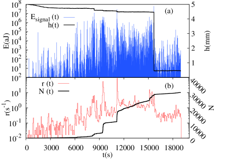
Figure 1: (color online) (a) Example of the outcome of a compression experiment at $R=1.6$ kPa/s, showing the change in the specimen’s height $h$ versus time (proportional to stress) and the energy of the AE avalanches, in logarithmic scale. (b) Time evolution of the AE activity rate and of the total number of events.

Fig. 2 shows the histograms that estimate the probability densities of the energiesSalje ; Baro_Vives , considering time windows of $3\times 10^{3}$s. All the distributions show a power-law behavior $p(E)\propto E^{-\epsilon}$, with an exponent in the range $\epsilon=1.40\pm 0.05$, stable for the whole experiment; this is the signature of a remarkable stationarity in the energy dissipation, which appears as independent of applied stress, in contrast to previous works Alava_review (therefore, the apparent non-stationarity of $E$ in Fig. 1 is due to a much larger number of events in the central part). The value of the exponent (obtained by maximum likelihood (ML) estimation Baro_Vives ) holds for about 7 decades and is robust against the thresholding of the data (fitting only values of $E$ larger than $E_{min}$) and quite independent of $R$, as shown in the inset of Fig. 2 Salje ; Baro_Vives ; smalldev . Although the resulting exponent turns out to be below the most accepted value for earthquakes, $\epsilon\simeq 1.67$, Kagan has noticed that this value is inflated due to systematic biases and one could instead expect $\epsilon$ close to 1.5 (i.e., $b\simeq 3/4$) Kagan_tectono10 . Reciprocally, systematic biases of the energy cannot be completely ruled out in AE experiments Alava_review ; Bonamy .

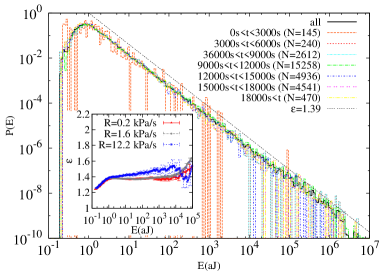
Figure 2: (color online) Distribution of avalanche energies during the full experiment with $R=1.6$ kPa/s and during 7 different subperiods. The line shows the behavior corresponding to $\epsilon=1.39$. The inset shows the ML-fitted exponent $\epsilon$ as a function of a lower threshold $E_{min}$ for the three experiments.

The next step in our analysis has been the computation of the number of aftershocks (AS) in order to compare with Omori’s law for earthquakes. We have considered as mainshocks (MS) all the events with energies in a certain predefined energy interval. After eachMS we study the sequence of subsequent events until an event with an energy larger than the energy of the MS is found, which finishes the sequence of AS. Then we divide the time line from the MS towards the future in intervals, for which we count the number of AS in each of them. Averages of the different sequences corresponding to all MS in the same energy range are performed, normalizing each interval by the number of sequences that reached such a time distance. The results presented in Figs.  3(a-c) show that the tendency to follow Omori’s law is clear, in some cases for up to 6 decades, with an exponent $p=0.75\pm 0.10$. (compare with Ref. Sornette_Ouillon ). Foreshocks, obtained in an analogous way, show a similar behavior, with a slightly smaller value of $p$.

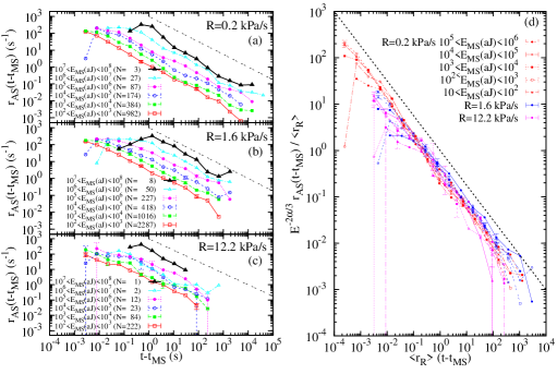
Figure 3: (color online) Number of aftershocks per unit time, $r$, as a function of the time distance to the main shock. MS are defined as the events in the energy range indicated by the legend. $n$ values indicate the number of sequences analyzed for each range. The dashed line indicates the Omori’s behavior with slope $-0.75$. Rescaled Omori plot showing the fulfillment of the productivity law, with $\alpha\simeq 0.5$.

The previous Omori’s plot allows also to estimate the exponent $\alpha$ of the productivity law, by rescaling the vertical axis with $E^{2\alpha/3}$, finding the optimum $\alpha$ which leads to the collapse of the data; i.e., $r_{AS}/E^{2\alpha/3}$ should be only a function of the time since the mainshock. The results in Fig. 3(d) show that $\alpha=0.5\pm 0.1$. This is again somewhat smaller than the counterpart for earthquakes, but the drift is compatible with the one found for the energy distribution, in other words, the ratio of exponents $(\epsilon-1)/\alpha$ is the same. Remarkably, a collapse can be obtained not only for mainshocks of different energies in the same experiment but also across experiments with different $R$, rescaling $r_{AS}$ as $r_{AS}E^{-2\alpha/3}/\langle r_{R}\rangle$, and the time since the MS, $t-t_{MS}$, as $(t-t_{MS})\langle r_{R}\rangle$, with $\langle r_{R}\rangle$ giving the mean number of events per unit time (see the figure).

These results already suggest that there is a certain similarity in the correlation between avalanches that extends from geophysical scales of the order of hundreds of km to our small samples with cracks much smaller than the mm scale. To deepen into the comparison we have proceeded to the analysis of the interevent or waiting times, defined as $\delta_{j}=t_{j}-t_{j-1}$, with $j$ labeling only the events with energy larger than a given $E_{min}$. The estimations of the waiting-time probability densities, $D(\delta;E_{min})$, for different $E_{min}$ and different experiments are shown in Fig. 4(a), displaying a power-law decay with exponent $1-\nu=0.93\pm 0.05$ for most of the time range, as implied by the Omori’s law. In order to compare the shape of the distributions we rescale the axes as $\langle r(E_{min})\rangle\delta$ and $D(\delta;E_{min},R)/\langle r(E_{min})\rangle$, with $\langle r(E_{min})\rangle$ giving the mean number of events per unit time with $E\geq E_{min}$. Fig. 4(b) shows how the different distributions collapse into a single one, signaling the existence of a scaling law; for a single experiment, as the activity rate verifies the Gutenberg-Richter law, the collapse “unifies” this law with the temporal properties Bak.2002 . For different experiments the collapse implies the similarity versus the compression rate $R$. Moreover, the plot also shows that a second power law emerges for the rightmost tail of the distributions, with an exponent $2+\xi=2.45\pm 0.08$ footnote .

To make clear the correspondence with earthquakes Fig. 4(b) also includes seismic data for different spatial windows in Southern California Bak.2002 ; Corral_physA.2004 . Although the previously reported value of $\xi$ for earthquakes Corral_physA.2004 is a bit smaller than for the experiment, the similarity is remarkable, taking into account that the earthquake measurements are taken over different spatial windows, whereas for the AE data we do not have access to such degrees of freedom.

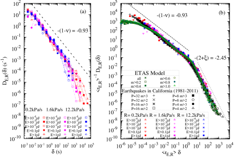
Figure 4: (color online) (a) Distribution of waiting times for different values of $E_{min}$ and the compression rate $R$. (b) The same data under rescaling, including also the results of the ETAS model and earthquakes from Southern-California divided into $P\times P$ regions Bak.2002 ; Corral_physA.2004 for the period Jan 1984 – Jun 2011.

How can we get then essentially the same behavior in such different situations? The answer lies in the variations of the activity rate. Let us consider a single Omori sequence, for which the waiting-time density depends on the background activity rate $\mu$ through a scaling form Corral_Christensen ,

$$D(\delta|\mu)=\frac{\mu}{(\mu\delta)^{1-\nu}}f(\mu\delta),$$ (1)

where $\nu$ is close to 0 and $f$ can be a decreasing exponential, or another function showing the same behavior at $0$ and $\infty$. If the background rate is not fixed but evolves during the experiment, the resulting density will be

$$D(\delta)\propto\int_{\mu_{min}}^{\mu_{max}}d\mu\rho(\mu)\mu D(\delta|\mu),$$ (2)

where $\rho(\mu)$ is the density of background rates. Substituting the previous equation and considering that $\mu$ is distributed between $\mu_{min}$ and $\mu_{max}$ with $\rho(\mu)\propto 1/\mu^{1-\xi}$ leads to $D(\delta)\propto 1/\delta^{1-\nu}$ for $\delta\ll\mu_{max}^{-1}$ (because the rescaled integral goes to zero as $\delta^{1+\xi+\nu}$) but $D(\delta)\propto 1/\delta^{2+\xi}$ for $\delta\gg\mu_{max}^{-1}$ (because the rescaled integral converges to a constant). This behavior for $\rho(r)$ can arise from a time evolution of the form $\mu(t)\propto t^{1/\xi}$, as $\rho(\mu)\propto|dt/d\mu(t)|$ Corral_Christensen . So, when the background rate varies across different scales (as in Fig. 1(b)) and this takes place through a power law, a second power law arises in $D(\delta)$. The experimental outcome suggests then $\xi\simeq 0.5$. We have simulated the Epidemic Type Aftershock (ETAS) model Helmstetter_Sornette_jgr02 , defined by the fact that each earthquake $i$, with a Gutenberg-Richter energy, triggers a sequence with a rate equal to $K{E_{i}}^{2\alpha/3}/(c+t-t_{i})^{1+\theta}$, and the overall rate is the linear superposition of these rates plus a background rate. The “microscopic” exponent $1+\theta$ corresponds to an observable $p=1-\theta$ Helmstetter_Sornette_jgr02 . Using as input the experimental values of $\epsilon$, $p$, and $\alpha$, together with $c=0.001$ s, and $\mu$ increasing slowly as $\mu(t)\propto 1-\cos\omega t$ (essentially a power law with $\xi=1/2$) we obtain very good concordance with the previous calculations (see Fig. 4(b)) when the branching ratio (given by $Kb/(\theta c^{\theta}(b-\alpha))$) is very close to criticality, i.e. 0.99. Also, the measurement of $r(t)$, using different time intervals, leads to a distribution with a power-law tail of the form $1/\sqrt{r}$ for small $r$ (not shown). This explanation could hold also for Ref. Santucci_Vanel_Ciliberto .

In summary, we have presented experimental results on the compression of a highly porous material, obtaining good fulfillment of some fundamental laws of statistical seismology. Laws involving the measurement of energy and the Omori’s law show some bias in the exponent with respect the earthquake case, whereas for the unified scaling law the quantitative agreement is much better. As our experiment does not allow the measurement of the location of the events, it has been not possible to test laws regarding spatial properties, which constitute also an important body of knowledge for the characterization of seismicity Grob . However, the validity of the unified scaling law in our experiments is associated to temporal variations of the background activity rate, rather than to spatial variations.

We acknowledge financial support from the Spanish Ministry of Science (MAT2010-15114), and the Austrian Science Fund (FWF) P23982-N20.

References

- (1) Y. Ben-Zion, Rev. Geophys. 46, RG4006, (2008).
- (2) I. Main., Rev. Geophys. 34, 433–462, (1996).
- (3) K. Mogi, Bull. Earthquake Res. Inst. 40, 125–173, (1962).
- (4) C. H. Scholz, Bull. Seismol. Soc. Am. 58, 1117–1130, (1968).
- (5) D. Bonamy, J. Phys. D: Appl. Phys. 42, 214014, (2009).
- (6) L. Girard, J. Weiss, and D. Amitrano Phys. Rev. Lett. 108, 225502, (2012).
- (7) T. Utsu, Pure Appl. Geophys. 155, 509–535, (1999).
- (8) M. J. Alava, P. K. V. V. Nukala, and S. Zapperi, Adv. Phys. 55, 349–476, (2006).
- (9) J. Davidsen, S. Stanchits, and G. Dresen, Phys. Rev. Lett. 98, 125502, (2007).
- (10) J. B. Rundle, D. L. Turcotte, R. Shcherbakov, W. Klein, and C. Sammis, Rev. Geophys. 41, 1019, (2003).
- (11) P. Bak, How Nature Works, The Science of Self-Organized Criticality, Copernicus, New York, (1996).
- (12) D. Sornette, Critical Phenomena in Natural Sciences, Springer, Berlin, 2nd edition, (2004).
- (13) J. P. Sethna, K. A. Dahmen, and C. R. Myers, Nature 418, 242–250, (2001).
- (14) T. Utsu, Y. Ogata, and R. S. Matsu’ura, J. Phys. Earth 43, 1–33, (1995).
- (15) T. Hirata, J. Geophys. Res. 92 B, 6215–6221, (1987).
- (16) A. Corral and K. Christensen, Phys. Rev. Lett. 96, 109801, (2006).
- (17) P. Bak, K. Christensen, L. Danon, and T. Scanlon, Phys. Rev. Lett. 88, 178501, (2002).
- (18) A. Corral, Physica A 340, 590–597, (2004).
- (19) A. Corral, Phys. Rev. Lett. 92, 108501, (2004).
- (20) A. Saichev and D. Sornette, Phys. Rev. Lett. 97, 078501, (2006).
- (21) A. Helmstetter, Phys. Rev. Lett. 91, 058501, (2003).
- (22) J. Weiss and M. C. Miguel, Mat. Sci. Eng. A 387-389, 292–296, (2004).
- (23) K. Mogi, Tectonophys. 5, 35–55, (1967).
- (24) J. Åström et al., Phys. Lett. A 356, 262–266, (2006).
- (25) M. Grob et al., Pure Appl. Geophys. 166, 777–799, (2009).
- (26) E. K. H. Salje et al., Phil. Mag. Lett. 91, 554–560, (2011).
- (27) J. Baró and E. Vives, Phys. Rev. E 85, 066121, (2012).
- (28) The small deviation corresponding to the largest compression rate kPa/s can be due to some non-trivial effects of overlapping and/or distortion of the avalanches.
- (29) Y. Y. Kagan, Tectonophys. 490, 103–114, (2010).
- (30) D. Sornette and G. Ouillon, Phys. Rev. Lett. 94, 038501, (2005).
- (31) On the other hand, if we restrict to stationary conditions (constant activity rate) the behavior is then similar to that of Refs. Davidsen_fracture ; Astrom ; Corral_prl.2004 .
- (32) A. Helmstetter and D. Sornette, J. Geophys. Res. 107 B, 2237, (2002).
- (33) S. Santucci, L. Vanel, and S. Ciliberto, Eur. Phys. J. Special Top. 146, 341–356, (2007).