Confinement in high- temperature lattice gauge theories

Abstract:

There has been substantial progress in understanding a class of SU(N) gauge theories that are confining at high temperatures. This class includes theories with center-symmetric Polyakov loop deformations or with periodic adjoint fermions. The crucial role of monopoles in lattice gauge theories of this type can be understood analytically. The basic mechanisms occur in the two-dimensional O(3) spin model, deformed by appropriate mass term to give an XY model. Vortices of the XY model are constituents of O(3) instantons just as SU(N) magnetic monopoles are constituents of KvBLL instantons. Similar methods applied to an SU(2) lattice gauge theory yield an effective U(1) description in which monopoles are responsible for confinement.

1 High-$T$ confinement on $R^{3}\times S^{1}$

It is now possible to construct four-dimensional gauge theories for which confinement may be reliably demonstrated using semiclassical methods [1, 2]. Essentially, these models exhibit confinement at high temperature. All of the models in this class have one or more small compact directions, and the methods and concepts are largely taken from finite the physics of gauge theories at finite temperature. These models combine the effective potential for the Polyakov loop $P$, $Z(N)$ center symmetry, instantons, and monopoles into a satisfying picture of confinement. At temperature $T\gg\Lambda$, we have $g^{2}\left(T\right)\ll 1$ so semiclassical methods may be used reliably. The one-loop effective potential for the Polyakov loop shows that gauge theories are generally in the deconfined phase at high $T$. However, it is possible to regain the confined phase by modifying the action. This leads to a perturbative calculation of possible phase structures, which turns out to be very rich, as well as a perturbative understanding of Polyakov loop physics in the confined phase. Furthermore, there is a non-perturbative mechanism for confinement, as measured by spatial Wilson loops. In this confinement mechanism, a key role is played by finite-temperature instantons, also known as calorons, and their monopole constituents.

The simplest approach to restoring confinement at high $T$ deforms the pure gauge theory by adding additional terms to the gauge action [1, 3, 4]. For $SU(2)$, a deformation of the form

$$S\rightarrow S-\beta\int d^{3}x\,H_{A}Tr_{A}P\left(\vec{x},x_{4}\right)$$ (1)

can be used, where the value of $x_{4}$ is arbitrary. If the coefficient $H_{A}$ is sufficiently negative, the deformation will counteract the effects of the one-loop effective potential, and $Z(N)$ symmetry will hold for large $T$. The schematic form of the phase diagram in the $T-H_{A}$ plane for an $SU(2)$ gauge theory with a deformation of either type is shown in Fig. 1. Positive values of $H_{A}$ favor $Z(2)$ symmetry-breaking, and the critical temperature will decrease as $H_{A}$ increases. In the limit $H_{A}\rightarrow\infty$, the Polyakov loops will only take on values in $Z(2)$; this is therefore an Ising limit. On the other hand, negative values of $H_{A}$ favor $Tr_{F}P=0$. This leads to a rise in the critical temperature. For the specific deformation considered here, the critical line switches to first-order behavior at a tricritical point. This is familiar but non-universal behavior in $Z(2)$ models [5]. For sufficiently negative $H_{A}$, we reach the semiclassical region where the running coupling $g(T)$ is small and semiclassical methods may be applied reliably. The right-hand axis shows the correspondence with an alternative approach to restoring confinement, adjoint fermions [2], as the fermion mass is varied.

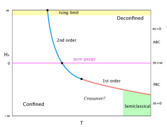
Figure 1: $SU(2)$ phase diagram

The analysis of instanton effects in this model is based on Polyakov’s study of the Georgi-Glashow model in three dimensions [6]. This is an $SU(2)$ gauge model coupled to an adjoint Higgs scalar, a role that is played in the four-dimensional theory by $A_{4}$. The monopole solutions of the field equations in four dimensions are instantons in three dimensions. Polyakov showed that a gas of such three-dimensional monopoles gives rise to non-perturbative confinement in three dimensions, even though the theory appears to be in a Higgs phase perturbatively. This analysis carries over to four-dimensional theories that are confined at high $T$.

2 $O(3)$ model in $d=2$

It is natural to ask if the continuum methods and results have parallels in lattice gauge theory. We illustrate how lattice theories handle topological content using the two-dimensional $O(3)$ model. Like QCD, this is an asymptotically free theory that has instantons [7]. As in finite temperature QCD, instantons can be decomposed into constituents [8]. In the case of the $O(3)$ model, these constituents can be identified with XY-model vortices [9]. In Fig. 2, a classical instanton solution is shown, with the arrows denoting the field components in the $\sigma_{1}-\sigma_{2}$ plane, and the colors denoting the value of $\sigma_{3}$. The embedding of the vortex-antivortex solution within the instanton is obvious.

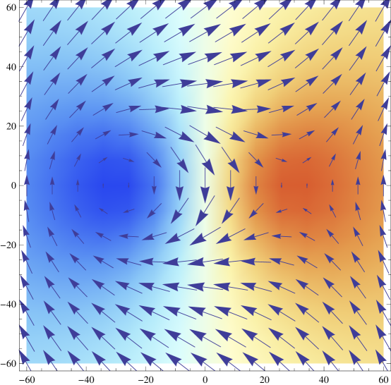
Figure 2: Instanton solution in $O(3)$ model.

The $O(3)$ model can be deformed into an XY model by the addition of a mass term for $\sigma_{3}$ [9, 10, 11]:

$$S\rightarrow S+\int d^{2}x\,\frac{1}{2}h\sigma_{3}^{2}$$ (2)

in a manner similar to finite-temperature QCD. The mass term breaks the classical conformance invariance of the model and makes it effectively Abelian at large distances. It is physically obvious that as $h$ increases, the deformed $O(3)$ model will become more and more like an XY model, and the constituent vortices inside instantons should be identified with the Kosterlitz-Thouless vortices of the XY model. To make this identification precise, we consider a lattice form of the deformed $O(3)$ model.

The lattice action is given by

$$S=-\sum_{x,\mu}K\vec{\sigma}(x)\cdot\vec{\sigma}(x+\mu)+\sum_{x}\frac{1}{2}h\sigma_{3}^{2}(x)$$ (3)

where $x$ is now a lattice site and $\mu$ one of two lattice directions. We parametrize $\vec{\sigma}$ as

$$\vec{\sigma}=\left(\sqrt{1-\sigma_{3}^{2}}\cos\theta,\sqrt{1-\sigma_{3}^{2}}\sin\theta,\sigma_{3}\right).$$ (4)

We can decompose the action as

$$S=-\sum_{x,\mu}K_{eff}\left(x,\mu\right)\cos\left[\theta\left(x\right)-\theta\left(x+\mu\right)\right]+S_{3}$$ (5)

where

$$K_{eff}\left(x,\mu\right)=K\sqrt{1-\sigma_{3}^{2}\left(x\right)}\sqrt{1-\sigma_{3}^{2}\left(x+\mu\right)}$$ (6)

and

$$S_{3}=-\sum_{x,\mu}K\sigma_{3}(x)\sigma_{3}(x+\mu)+\sum_{x}\frac{1}{2}h\sigma_{3}^{2}(x)$$ (7)

both depend only on $\sigma_{3}$.

At this point, we can follow well-known arguments to obtain a form for the model that explicitly includes vortex effects [12]. We write the partition function as

$$Z=\int_{S^{2}}\left[d\sigma\right]e^{-S}=\int_{-1}^{+1}\left[d\sigma_{3}\left(x\right)\right]e^{-S_{3}}\int_{S^{1}}\left[d\theta\right]\prod_{x,\mu}e^{K_{eff}\left(x,\mu\right)\cos\left(\nabla_{\mu}\theta\left(x\right)\right)}$$ (8)

where $\nabla_{\mu}\theta\left(x\right)\equiv\theta(x+\mu)-\theta(x)$. For each link, we expand the interaction in a character expansion, which is a Fourier series:

$$Z=\int_{-1}^{+1}\left[d\sigma_{3}\left(x\right)\right]e^{S_{3}}\int_{S^{1}}\left[d\theta\right]\prod_{x,\mu}\sum_{n_{\mu}\left(x\right)\in Z}I_{n_{\mu}\left(x\right)}(K_{eff}\left(x,\mu\right))e^{in_{\mu}\left(x\right)\nabla_{\mu}\theta\left(x\right)}$$ (9)

where $I_{n}$ is a modified Bessel function. This step introduces integer variables $n_{\mu}\left(x\right)$ on every link. We now make use of the asymptotic form of $I_{n}$ for $K_{eff}\gg 1$, using what is called the Villain approximation, obtaining

$$Z=\int_{-1}^{+1}\left[d\sigma_{3}\left(x\right)\right]e^{S_{3}}\int_{S^{1}}\left[d\theta\right]\prod_{x,\mu}\sum_{n_{\mu}\left(x\right)\in Z}\frac{1}{\sqrt{2\pi K_{eff}\left(x,\mu\right)}}e^{K_{eff}\left(x,\mu\right)-n_{\mu}^{2}\left(x\right)/2K_{eff}\left(x,\mu\right)}e^{in_{\mu}\left(x\right)\nabla_{\mu}\theta\left(x\right)}$$ (10)

Although this step appears here as an approximation, it is really a small deformation of the action that does not change the critical properties of the model. It is now easy to integrate over the $\theta$ variables, which leads to the constraint$\nabla_{\mu}n_{\mu}\left(x\right)=0$. This in turns allows us to write $n_{\mu}(x)=\epsilon_{\mu\nu}\nabla_{\nu}m(X)$ where $m\left(X\right)$ is an integer-valued field on the dual lattice site $X$ which is displaced from $x$ by half a lattice spacing in each direction. The partition function is now

$$Z=\int_{-1}^{+1}\left[d\sigma_{3}\left(x\right)\right]e^{-S^{\prime}_{3}}\sum_{\{m\left(X\right)\}\in Z}e^{-\sum_{X,\nu}\left(\nabla_{\nu}m\left(X\right)\right)^{2}/2K_{eff}\left(x,\mu\right)}$$ (11)

where

$$S^{\prime}_{3}=S_{3}-\sum_{x,\mu}\left[K_{eff}\left(x,\mu\right)-\frac{1}{2}\log\left(2\pi K_{eff}\left(x,\mu\right)\right)\right]$$ (12)

The final step is to introduce a new field $\phi(x)\in R$ using a periodic $\delta$-function, effectively performing a Poisson resummation:

$$Z=\int_{-1}^{+1}\left[d\sigma_{3}\left(x\right)\right]e^{S^{\prime}_{3}}\int_{R}\left[d\phi\left(X\right)\right]e^{-\sum_{X,\nu}\left(\nabla_{\nu}\phi\left(X\right)\right)^{2}/2K_{eff}\left(x,\mu\right)}\sum_{\{m\left(X\right)\}\in Z}e^{2\pi im\left(X\right)\phi\left(X\right)}.$$ (13)

We see from this form of the partition function that vortices are explicitly present in the functional integral, induced by source $m(X)$ on the dual lattice. For each configuration $\{m\left(X\right)\}$, the integral over $\phi$ and $\sigma_{3}$ must be carried out. This can be done using standard perturbative methods. Each dual lattice site $X$ where $m(X)\neq 0$, will be the site of a vortex of charge $m(X)$. In a dilute gas approximation, we can see that the size of the vortex core will in general be set by the scale-setting parameter $h$, which determines the region around $X$ where $\sigma_{3}$ is significantly different from zero. The contribution of the vortex core to the total weight of a given configuration $\{m\left(X\right)\}$ can be captured in a vortex activity $y$, which represents the Boltzmann weight of the classical lattice vortex solution times a functional determinant factor, just as in the continuum. It is clear that in the limit where $h$ is very large, $\sigma_{3}$ will be essentially zero everywhere, and we recover the $XY$ model with $K_{eff}\simeq K$ and a vortex core size on the order of the lattice spacing. Note that the $Z(2)$ symmetry under $\sigma_{3}\rightarrow-\sigma_{3}$ means that for each vortex winding number $m$, there are two types of vortices depending on the behavior of $\sigma_{3}$ in the core, as in the continuum. For $h>0$, the large-distance behavior is that of an XY model, giving a continuous path between the $O(3)$ model and the vortex Coulomb gas phase of the XY model. If we keep only the $m=1$ contributions, we have essentially a lattice sine-Gordon model

$$Z=\int_{R}\left[d\phi\left(X\right)\right]\exp\left[-\sum_{X,\mu}\frac{1}{2\bar{K}_{eff}}\left(\nabla_{\mu}\phi\left(X\right)\right)^{2}+\sum_{X}4y\cos\left(2\pi\phi\left(X\right)\right)\right]$$ (14)

where $\bar{K}_{eff}$ is the value of $K_{eff}$ away from the vortex cores. All of the physics associated with the short-ranged $\sigma_{3}$ field is contained in $\bar{K}_{eff}$ and $y$.

3 High-T confinement for lattice $SU(2)$ in $d=4$

The $(3+1)$-dimensional $SU(2)$ gauge theory at high temperatures can be treated in much the same way as the two-dimensional $O(3)$ model. It is convenient to work in Polyakov gauge, where $A_{4}$ is diagonal and time-independent so that the Polyakov loop is given by $P=\exp\left(iA_{4}/T\right)=\exp\left(i\theta\tau_{3}\right)$. A sufficiently strong deformation term will make the expected value of the timelike link variable $U_{4}=\exp(iA_{4})$ significantly different from one. This in term will give large masses to the off-diagonal parts of the $U_{j}$ fields. The off-diagonal fields will be important only inside monopole cores where $A_{4}$ is small. Outside monopole cores, the model is effectively Abelian.

A simplified approach is to take the deformation term to be very strong and assume that all the fields are independent of $x_{4}$. We take the the timelike links $U_{4}\left(\vec{x,}t\right)$ to be diagonal and independent of $t$: $U_{4}\left(\vec{x}\right)=\exp\left(i\tau_{3}\theta_{0}\left(\vec{x}\right)\right)$. A strong deformation term forces $\left\langle Tr_{F}P\right\rangle=0$ with an expected value for $\left\langle\theta_{0}\right\rangle$, given by $N_{t}\left\langle\theta_{0}\right\rangle=\pi/2$. As in the $O(3)$ case, we can define the (dimensionally-reduced) spatial gauge fields as

$$U_{j}\left(\vec{x}\right)=\sqrt{1-\left(U_{j}^{1}\left(\vec{x}\right)\right)^{2}-\left(U_{j}^{2}\left(\vec{x}\right)\right)^{2}}\exp\left(i\tau_{3}\theta_{j}\left(\vec{x}\right)\right)+i\tau_{1}\cdot U_{j}^{1}\left(\vec{x}\right)+i\tau_{2}\cdot U_{j}^{2}\left(\vec{x}\right)$$ (15)

The expectation value $\left\langle U_{0}\right\rangle$ makes the $U_{j}^{1}$ and $U_{j}^{2}$ fields massive, and they do not contribute to the large-distance behavior. This leaves us with an effective three-dimensional $U(1)$ gauge theory. The dual of a a three-dimensional Abelian gauge theory is an Abelian spin system, in this case again yielding a lattice sine-Gordon model as in the continuum [13].

The above simplified approach, based on the early application of dimensional reduction, is in fact too simple. As in the $O(3)$ model, where there were two types of vortices and two types of antivortices distinguished by their behavior in the vortex core, there are four Eucldean monopole solutions, not two [14, 15, 16, 17]. The BPS-type monopole and anti-monopole solutions can be constructed as conventional time-independent monopole solutions, and are thus included in the simplified approach. On the other hand, the KK-type solutions are constructed from the BPS solutions using an $x_{4}$-dependent, non-periodic gauge transformation that changes the instanton charge of a field configuration[17]. Thus, a proper treatment of both types of monopoles is necessary. After accounting carefully for both types of solutions, the dual form of the partition function in the confined phase is

$$Z=\int_{R}\left[d\phi\left(X\right)\right]\exp\left[-\sum_{X,\mu}\frac{g^{2}}{8N_{t}}\left(\nabla_{\mu}\phi\left(X\right)\right)^{2}+\sum_{X}4y\cos\left(2\pi\phi\left(X\right)\right)\right]$$ (16)

which has the same form as the corresponding continuum result, where the effective action has the form

$$S_{eff}=\int d^{3}x\left[\frac{g^{2}(T)T}{32\pi^{2}}\left(\partial_{j}\phi\right)^{2}-4y\cos(\phi)\right].$$ (17)

The two results are equivalent after identifying $T^{-1}$ with $N_{t}$ and rescaling the $\phi$ field.

4 Conclusions

We have seen that non-Abelian lattice theories deformed to Abelian effective theories work in the same way as their continuum counterparts, and lattice duality reproduces semiclassical continuum duality in these cases. In the case of $SU(2)$ lattice gauge theory, there is a continuous path between the confined phase of SU(2) and the monopole-dominated phase of lattice U(1) gauge theory. The lattice theories know something about continuum topology, but care must be exercised. One particularly interesting feature of the lattice analysis is that the construction works for $O(N)$ models with $N>3$ when a term of the form

$$\sum_{x}\frac{1}{2}h\sum_{j=3}^{N}\sigma_{j}^{2}(x)$$ (18)

is added to the lattice action. It is clear on physical grounds that all the $O(N)$ models should reduce to an XY model at large distances when deformed appropriately. However, instantons only appear in the $O(3)$ model. It is apparent that not all non-perturbative contributions are clearly associated with instantons and that instanton methods are in some sense incomplete prescriptions for determining the non-perturbative content of a theory; see the recent work of Argyres and Unsal for a related continuum perspective [18, 19].

References

- [1] J. C. Myers and M. C. Ogilvie, Phys. Rev. D 77, 125030 (2008) [arXiv:0707.1869 [hep-lat]].
- [2] M. Unsal, Phys. Rev. Lett. 100, 032005 (2008) [arXiv:0708.1772 [hep-th]].
- [3] M. C. Ogilvie, P. N. Meisinger and J. C. Myers, PoS LAT 2007, 213 (2007) [arXiv:0710.0649 [hep-lat]].
- [4] M. Unsal and L. G. Yaffe, Phys. Rev. D 78, 065035 (2008) [arXiv:0803.0344 [hep-th]].
- [5] H. Nishimura and M. C. Ogilvie, Phys. Rev. D 85, 065021 (2012) [arXiv:1111.6101 [hep-th]].
- [6] A. M. Polyakov, Nucl. Phys. B 120, 429 (1977).
- [7] A. M. Polyakov, Phys. Lett. B 59, 79 (1975).
- [8] D. J. Gross, Nucl. Phys. B 132, 439 (1978).
- [9] M. C. Ogilvie and G. S. Guralnik, Nucl. Phys. B 190, 325 (1981).
- [10] I. I. Satija and R. Friedberg, Nucl. Phys. B 200, 457 (1982).
- [11] I. Affleck, Phys. Rev. Lett. 56, 408 (1986).
- [12] J. V. Jose, L. P. Kadanoff, S. Kirkpatrick and D. R. Nelson, Phys. Rev. B 16, 1217 (1977).
- [13] T. Banks, R. Myerson and J. B. Kogut, Nucl. Phys. B 129, 493 (1977).
- [14] T. C. Kraan and P. van Baal, Phys. Lett. B 428, 268 (1998) [hep-th/9802049].
- [15] T. C. Kraan and P. van Baal, Nucl. Phys. B 533, 627 (1998) [hep-th/9805168].
- [16] K. -M. Lee and C. -h. Lu, Phys. Rev. D 58, 025011 (1998) [hep-th/9802108].
- [17] N. M. Davies, T. J. Hollowood, V. V. Khoze and M. P. Mattis, Nucl. Phys. B 559, 123 (1999) [hep-th/9905015].
- [18] P. Argyres and M. Unsal, Phys. Rev. Lett. 109, 121601 (2012) [arXiv:1204.1661 [hep-th]].
- [19] P. C. Argyres and M. Unsal, JHEP 1208, 063 (2012) [arXiv:1206.1890 [hep-th]].