Some results about ergodicity in shape for a crystal growth model

Abstract

We study a crystal growth Markov model proposed by Gates and Westcott ([1], [2]). This is an aggregation process where particles are packed in a square lattice accordingly to prescribed deposition rates. This model is parametrized by three values $(\beta_{i},~{}i=0,1,2)$ corresponding to depositions on three different types of sites. The main problem is to determine, for the shape of the crystal, when recurrence and when ergodicity do occur. In [3] and [4] sufficient conditions are given both for ergodicity and transience. We establish some improved conditions and give a precise description of the asymptotic behavior in a special case.

1 Definitions and first properties

Let $n$ be an integer, $n\geq 2$. We consider a set of $n$ aligned sites, each site corresponding to a growing pile of particles. The state of a lamellar crystal (see [5]) is described by a vector $x=(x(1),\dots,x(n))\in\mathbb{N}^{n}$, where the value of $x(i)$ may be thought of as the height of the pile above site $i$. If $1\leq j\leq n$, $e_{j}$ will stand for the unitary vector:

$$e_{j}(i)=\delta_{i,j}.$$

For $x\in\mathbb{N}^{n}$ and $1\leq j\leq n$, let $V_{j}(x)$ be the number of sites adjacent to $j$ whose pile is strictly higher than the pile at site $j$. Namely,

$$V_{j}(x)=\mathds{1}_{\{x(j-1)>x(j)\}}+\mathds{1}_{\{x(j+1)>x(j)\}}\in\{0,1,2\}.$$

For $V_{j}(x)$ to be well-defined for $j=1$ and $j=n$, we adopt from now on the convention that $x(0)=x(n+1)=0$, unless otherwise specified. This is the so-called zero condition, which amounts to add a leftmost and a rightmost site that stay at height $0$ forever. Another natural convention is the periodic condition that consists in deciding that $x(0)=x(n)$ and $x(n+1)=x(1)$, but we believe that all the results here can be transposed to periodic condition (in the same way as Theorem 1.1 in [3]). We shall also use the infinite condition (resp. the zero-infinite condition), that is $x(0)=x(n+1)=\infty$ (resp. $x(0)=0,x(n+1)=\infty$), and anything relative to this condition will be denoted with the superscript $\infty$ (resp. the superscript $0/\infty$).

Definition 1.

Let $n\geq 2$ and $\beta=(\beta_{0},\beta_{1},\beta_{2})\in]0,+\infty[^{3}$. We say that $(X^{n}_{t},t\geq 0)$ is a crystal process with $n$ sites and parameter $\beta$ if it is a Markov process on $\mathbb{N}^{n}$ with transition rates given by

$$\begin{cases}q(x,x+e_{j})=\beta_{V_{j}(x)},&j=1,\dots,n,\\ q(x,y)=0,&\text{if }y\notin\{x+e_{1},\dots,x+e_{n}\}.\end{cases}$$

For a configuration $x$, we define the shape $h$ of $x$ by

$$h=\left(\Delta_{1}x,\dots,\Delta_{n-1}x\right),$$

where

$$\Delta_{j}x=x(j)-x(j+1),~{}j=1,\dots,n-1.$$

Knowing $h$ is equivalent to knowing $x$ up to vertical translation. It is important to remark that $V_{j}(x)$ only depends on $x$ through $h$, and $V_{j}(h)$ will denote the value of $V_{j}(x)$ for any $x$ whose shape is $h$. Let us define, for $j=1,\dots,n$, the vector

$$f_{j}=\begin{cases}e_{1},&\text{ if }j=1,\\ e_{j}-e_{j-1},&\text{ if }1<j<n,\\ -e_{n-1},&\text{ if }j=n.\end{cases}$$

The object of main interest is the process of the shape of $X^{n}$, that we now define, rather than the process $X^{n}$ itself.

Definition 2.

The shape process with $n$ sites and parameter $\beta$ is defined by

$$H^{n}_{t}=\left(\Delta_{1}X^{n}_{t},\dots,\Delta_{n-1}X^{n}_{t}\right),$$

where $X^{n}$ is a crystal process with $n$ sites and parameter $\beta$. $H^{n}$ is a Markov process on $\mathbb{Z}^{n-1}$ with transition mechanism given by

$$\begin{cases}q(h,h+f_{j})=\beta_{V_{j}(h)},&j=1,\dots,n,\\ q(h,h^{\prime})=0,&\text{if }h^{\prime}\notin\{h+f_{1},\dots,h+f_{n}\}.\end{cases}$$

These processes have a basic symmetry property, namely the process $(X^{n}_{t}(n),\dots,$ $X^{n}_{t}(1))$ has the same distribution as $X^{n}$, and consequently the process $(-\Delta_{n-1}X^{n},\dots$
$-\Delta_{1}X^{n})$ has the same distribution as $H^{n}$. There is a convenient construction of $X^{n}$, and hence of $H^{n}$, that we now describe and will later refer as the Poisson construction. As we will see later, the interest of this construction is to yield useful couplings. Let $b_{0}$, $b_{1}$ and $b_{2}$ be the $\beta_{k}$’s ranked in the increasing order. We take a family of Poisson processes $(N_{k,j},~{}0\leq k\leq 2,~{}1\leq j\leq n)$ such that

• $N_{k,j}$ has intensity $b_{k}$,

• the triples $(N_{0,j},N_{1,j},N_{2,j})_{1\leq j\leq n}$ are mutually independent,

• for any $j$ there exist three processes $\tilde{N}_{0,j},~{}\tilde{N}_{1,j}$ and $\tilde{N}_{2,j}$, mutually independent, with intensities $b_{0},~{}b_{1}-b_{0}$ and $b_{2}-b_{1}$ respectively, such that

  $$N_{0,j}=\tilde{N}_{0,j},\quad N_{1,j}=\tilde{N}_{0,j}+\tilde{N}_{1,j},\quad N_{2,j}=\tilde{N}_{0,j}+\tilde{N}_{1,j}+\tilde{N}_{2,j}.$$

We build the process $(X^{n}_{t},t\geq 0)$ starting from $x_{0}$ letting $X^{n}_{0}=x_{0}$, and at any jump time $t$ of some $N_{k,j}$,

$$X^{n}_{t}=\begin{cases}X^{n}_{t^{-}}+e_{j},&\text{ if }\beta_{V_{j}(X^{n}_{t^{-}})}\geq b_{k},\\ X^{n}_{t^{-}},&\text{otherwise.}\end{cases}$$ (1)

It is not hard to check that this process has the Markov property and the desired jump rates. Hence it is a crystal process starting from $x_{0}$ with $n$ sites and parameter $\beta$.
For any positive function $f$ on $\mathbb{N}$ or $\mathbb{R}_{+}$, we write

$$f(x)=\mathcal{O}_{exp}(x)$$

if there exists $\alpha,C>0$ such that $f(x)\leq Ce^{-\alpha x}$. If $f$ also depends on some other variable $t$, the notation

$$f(x,t)=\mathcal{O}_{exp}^{t}(x)$$

means that the same inequality holds with constants $C$ and $\alpha$ being independent of $t$.
We say that the process $X^{n}$ is ergodic in shape, resp. transient in shape, whenever the process $H^{n}$ is ergodic, resp. transient. The notation $\mathbb{P}_{x}$, resp. $\mathbb{P}_{h}$, will stand for the distribution of the trajectory $(X^{n}_{t},t\geq 0)$ starting from $x$, resp. of the trajectory $(H^{n}_{t},t\geq 0)$ starting from $h$. If there is any ambiguity on the parameter $\beta$, the notation $\mathbb{P}_{x}^{\beta}$ will be used instead. The null vector will be denoted by $\mathbf{0}$.
This simple model was first described by Gates and Westcott in [1], where attention was focused on the special case $\beta_{2}>\beta_{0}$, and

$$\beta_{1}=(\beta_{0}+\beta_{2})/2.$$

Under this assumption the process $H^{n}$ with periodic conditions enjoys a remarkable dynamic reversibility property that implies ergodicity, and even allows to derive an exact computation of the invariant distribution. Unfortunately without this assumption on $\beta$, there is no such simple way to determine whether ergodicity occurs or not. However we can make a naive remark: since $\beta_{0}$ is the statistic speed of peaks and $\beta_{2}$ is the one of holes, basic intuition says that increasing $\beta_{0}$ should make the shape more irregular, making the process $H^{n}$ more likely to be transient. Conversely, increasing $\beta_{2}$ should make the shape smoother, making the process $H^{n}$ more likely to be recurrent.
Gates and Westcott later proved several results about the problem of recurrence in shape for other parameters, by means of Foster criteria with quite simple Lyapunov functions. Theorem 2 in [4] states that for periodic conditions and $n\geq 2$, $H^{n}$ is transient if $\beta_{2}<\beta_{0}$. Ergodicity is shown to hold for

$$\beta_{1},\beta_{2}>(n-1)^{2}\beta_{0},$$ (2)

and a similar condition for ergodicity is also obtained for a process with a two-dimensional grid of sites. Of course when $n$ is large such conditions are very restrictive.
The family $(\Delta_{j}X^{n}_{t},t\geq 0)$ is said to be exponentially tight if

$$\mathbb{P}_{\mathbf{0}}(|\Delta_{j}X^{n}_{t}|\geq k)=\mathcal{O}_{exp}^{t}(k).$$

We also say that the family $(H^{n}_{t},t\geq 0)$ is exponentially tight if for $j=1,\dots n-1$, $(\Delta_{j}X^{n}_{t},t\geq 0)$ is exponentially tight. Obviously, exponential tightness of the process $(H^{n}_{t},t\geq 0)$ implies that it is ergodic with an invariant distribution having exponential tails.
From Theorem 1.2 in [3] we get:

Theorem 1.

If $n\geq 2$ and $\beta_{0}<\beta_{1}\leq\beta_{2}$ then $(H^{n}_{t},t\geq 0)$ is exponentially tight, and hence ergodic. Moreover there exists $d_{n}<\beta_{1}$ such that

$$\mathbb{P}_{\mathbf{0}}(X^{n}_{t}(n)\geq d_{n}t)=\mathcal{O}_{exp}(t).$$

We point out that this result is actually given for $\beta_{0}<\beta_{1}<\beta_{2}$ but the reader may verify that its proof works exactly the same if we take $\beta_{1}=\beta_{2}$. We will pick up several ideas of the approach in [3] in order to give weaker conditions for ergodicity in shape. Our notations will be consistent with this reference as much as possible. Before stating our results we begin by defining two useful notions: growth rate and monotonicity.

Proposition 1.

Suppose that $H^{n}$ is ergodic and let $\pi^{n}$ be its invariant distribution. There exists $v^{n}>0$ such that for $j=1,\dots,n$, almost surely,

$$\lim_{t\to\infty}\frac{X^{n}_{t}(j)}{t}=v^{n}.$$

Moreover, for any $j=1,\dots,n$, we have $v^{n}=\sum_{h\in\mathbb{Z}^{n-1}}\beta_{V_{j}(h)}\pi^{n}(h)$.

Proof.

Let $j\in\{1,\dots,n\}$. Since $(X^{n}_{t}(j),t\geq 0)$ is a counting process with intensity $\beta_{V_{j}(X^{n}_{t})}$, we have that

$$M_{t}:=X^{n}_{t}(j)-\int_{0}^{t}\beta_{V_{j}(X^{n}_{s})}\mathrm{d}s\text{ is a martingale},$$ (3)

and also

$$L_{t}:=M_{t}^{2}-\int_{0}^{t}\beta_{V_{j}(X^{n}_{s})}\mathrm{d}s\text{ is a martingale}.$$ (4)

Since ergodicity yields the a.s. convergence

$$\lim_{t\to\infty}\frac{1}{t}\int_{0}^{t}\beta_{V_{j}(X^{n}_{s})}\mathrm{d}s=\sum_{h\in\mathbb{Z}^{n-1}}\beta_{V_{j}(h)}\pi^{n}(h),$$

it now remains to show that $\lim t^{-1}M_{t}=0$, a.s.  But (3) allows us to use Doob’s inequality: for $r\leq t$,

$$\mathbb{P}\left(\sup_{s\in[r,t]}\frac{|M_{s}|}{s}\geq\varepsilon\right) \leq\mathbb{P}\left(\sup_{s\in[r,t]}|M_{s}|\geq r\varepsilon\right)$$

$$\leq\frac{\mathbb{E}[M_{t}^{2}]}{r^{2}\varepsilon^{2}}$$

$$\leq\frac{Kt}{r^{2}\varepsilon^{2}},$$

where $K=\max(\beta_{0},\beta_{1},\beta_{2})$. The last inequality is a direct consequence of (4). Thus we have $\mathbb{P}(\sup_{n^{2}\leq s\leq(n+1)^{2}}s^{-1}|M_{s}|\geq\varepsilon)\leq K(n+1)^{2}/(\varepsilon^{2}n^{4})$, and we may can conclude by Borel-Cantelli’s lemma. ∎

For $n=2$, the simplicity of the dynamics allows us to compute the exact value of the growth rate:

Proposition 2.

$H^{2}$ is ergodic if and only if $\beta_{1}>\beta_{0}$. In this case, $v^{2}=\frac{2\beta_{0}\beta_{1}}{\beta_{0}+\beta_{1}}$.

Proof.

$H^{2}_{t}=X^{2}_{t}(1)-X^{2}_{t}(2)$ is a random walk on $\mathbb{Z}$, whose jump rates are given by:

$$\begin{cases}q(i,i+1)=\beta_{0},~{}q(i,i-1)=\beta_{1},&\text{ if }i>0,\\ q(0,1)=q(0,-1)=\beta_{0},&\\ q(i,i+1)=\beta_{1},~{}q(i,i-1)=\beta_{0},&\text{ if }i<0.\end{cases}$$

Thus the first assertion is straightforward. If $\beta_{1}>\beta_{0}$, it is easy to check that the probability measure

$$\mu(\{i\})=\frac{\beta_{1}-\beta_{0}}{\beta_{1}+\beta_{0}}\left(\frac{\beta_{0}}{\beta_{1}}\right)^{|i|}$$

is a reversible measure for this random walk, so it is the invariant distribution of the process. We can then compute:

$$v^{2}=\sum_{i\in\mathbb{Z}}\pi_{2}(\{i\})(\beta_{0}\mathds{1}_{i\geq 0}+\beta_{1}\mathds{1}_{i<0})=\beta_{0}\pi^{2}(\mathbb{Z}_{+})+\beta_{1}\pi^{2}(\mathbb{Z}_{-}^{*})=\frac{2\beta_{0}\beta_{1}}{\beta_{0}+\beta_{1}}.$$

∎

We define the canonical partial order $\leq$ in an obvious way: for two configurations $x,y\in\mathbb{N}^{n}$, we write $x\leq y$ if

$$x(j)\leq y(j),~{}1\leq j\leq n.$$

The process $X^{n}$ is said to be attractive if for any $x\leq y$, there exists a coupling of two processes $(X^{n}_{t},t\geq 0)$ and $(Y^{n}_{t},t\geq 0)$, with distributions $\mathbb{P}_{x}$ and $\mathbb{P}_{y}$, such that almost surely,

$$\forall t\geq 0,~{}X^{n}_{t}\leq Y^{n}_{t}.$$

Lemma 1.

Let $n\geq 2$. If $\beta_{0}\leq\beta_{1}\leq\beta_{2}$, then $X^{n}$ is attractive.

Proof.

Let $x\leq y$. We consider $X^{n}$ and $Y^{n}$ obtained with the above Poisson construction, with $X^{n}_{0}=x$, $Y^{n}_{0}=y$, both using the same Poisson processes. Suppose that

$$X^{n}_{t^{-}}(j)=Y^{n}_{t^{-}}(j)$$

and $N_{k,j}$ jumps at time $t$. We then have $V_{j}(X^{n}_{t^{-}})\leq V_{j}(Y^{n}_{t^{-}})$. Consequently, if $X^{n}_{\cdot}(j)$ jumps at time $t$, then so does $Y^{n}_{\cdot}(j)$ and hence the inequality $X^{n}(j)\leq Y^{n}(j)$ is preserved. ∎

We are now interested in comparing two processes with same initial states, but different numbers of sites, or different parameters. In general it is not true that increasing one of the parameters increases the process himself. However we have a weaker result which is sufficient for our purpose.

Lemma 2.

Let $n\geq 2$ and $\beta\in]0,+\infty[^{3}$. If $\beta_{0}\leq\beta_{1}\leq\beta_{2}$ and $n\leq m$, then there exists a coupling of two processes $X^{n}$ and $X^{m}$ distributed as $\mathbb{P}_{x}^{\beta,n}$ and $\mathbb{P}_{x}^{\beta,m}$, such that

$$\forall t\geq 0,~{}X^{n}_{t}\leq X^{m}_{t}.$$

Let $\beta^{\prime}\in]0,+\infty[^{3}$. If $\beta$ and $\beta^{\prime}$ are such that $\beta_{k}\leq\beta^{\prime}_{\ell}$ for $k\leq\ell$, then there exists a coupling of two processes $X^{n}_{t}$ and $X^{\prime n}_{t}$ distributed as $\mathbb{P}_{x}^{\beta,n}$ and $\mathbb{P}_{x}^{\beta^{\prime},n}$, such that

$$\forall t\geq 0,~{}X^{n}_{t}\leq X^{\prime n}_{t}.$$

Proof.

Here again we can use Poisson constructions in such a way that the obtained processes enjoy the desired properties. The details are left to the reader. ∎

2 Results

As already noticed, $X^{n}$ is transient in shape (for periodic conditions) when $\beta_{2}<\beta_{0}$. This is not a surprise since this inequality says that peaks grow faster than holes. Our first Theorem describes more precisely the asymptotic behaviour of the process $X^{n}$, with zero-condition, under this assumption. It says that almost surely the shape ultimately adopts a comb shape. The exact form of the comb actually depends on the position of $\beta_{1}$ relatively to $\beta_{2}$ and $\beta_{0}$ so we actually establish three analogue results. To illustrate this we show three simulations showing realizations of $t^{-1}X^{n}_{t}$ for $t=1000$ and three different parameters.

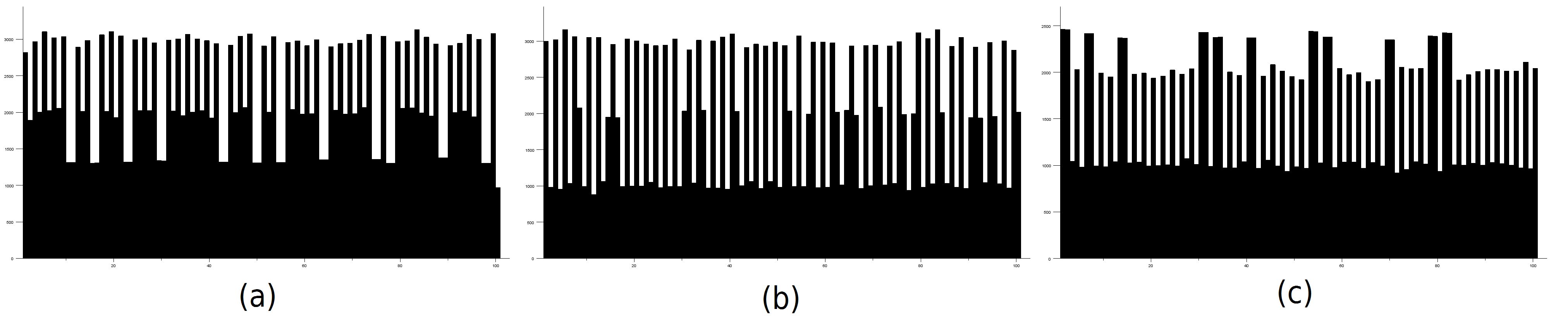
Figure 1: $X^{n}_{t}$ pour $n=100$, $t=1000$, et (a) $\beta=(3,1,2)$, (b) $\beta=(3,2,1)$, (c) $\beta=(2,3,1)$.

Before stating the result we need to introduce some further notation. We write $t^{-1}X^{n}_{t}$ for the vector $\left(t^{-1}X^{n}_{t}(1),\dots,t^{-1}X^{n}_{t}(n)\right)$. For two vectors $a=(a_{1},\dots a_{k})$ and $b=(b_{1},\dots b_{\ell})$ we denote by $(a,b)$ the vector $(a_{1},\dots a_{k},b_{1},\dots b_{\ell})$. $(-)$ denotes the empty vector. Let $\mathcal{E}_{1}$ be the set of all the $n$-uples of the form

$$(a_{1},\beta_{2},a_{2},\dots,a_{k-1},\beta_{2},a_{k}),$$ (5)

where $k\in\mathbb{N}$, and $a_{i}=(\beta_{0})\text{ or }(v^{2},v^{2})$ for $1\leq i\leq k$. Similarly we define $\mathcal{E}_{2}$ as the set of all the $n$-uples of the form

$$(\beta_{i_{1}},\dots\beta_{i_{n}}),$$ (6)

where $i_{j}\in\{0,1,2\}$, $i_{j}\neq i_{j+1}\text{ for }1\leq j\leq n-1$ and $i_{1},i_{n}\neq 2$. Let $H^{n,\infty}$ be the shape process with infinite condition. The proof of Proposition 2 also works with $H^{2}$ being replaced by $H^{2,\infty}$, $\beta_{0}$ by $\beta_{1}$ and $\beta_{1}$ by $\beta_{2}$. Thus, whenever $\beta_{2}>\beta_{1}$ the process $H^{2,\infty}$ is ergodic with growth rate $v^{2,\infty}=2\beta_{1}\beta_{2}/(\beta_{1}+\beta_{2})$. Let $\mathcal{E}_{3}$ be the set of all $n$-uples of the form

$$(e_{L},\beta_{0},a_{1},\beta_{0},a_{2},\dots,a_{k-1},\beta_{0},a_{k},\beta_{0},e_{R}),$$ (7)

where $k\in\mathbb{N}$, $a_{i}=(\beta_{2})\text{ or }(v^{2,\infty},v^{2,\infty})$ for $1\leq i\leq k$, and $e_{L},e_{R}=(\beta_{1})$ or $(-)$.
In Section 3 we prove:

Theorem 2.

Let $n\geq 2$ and $x\in\mathbb{Z}^{n}$.

• If $\beta_{2}<\beta_{0}\leq\beta_{1}$ then $t^{-1}X^{n}_{t}$ converges $\mathbb{P}_{x}$-a.s. and

  $$\mathbb{P}_{x}\left(\lim_{t\to\infty}t^{-1}X^{n}_{t}\in\mathcal{E}_{1}\right)=1.$$

• If $\beta_{2}<\beta_{1}<\beta_{0}$ then $t^{-1}X^{n}_{t}$ converges $\mathbb{P}_{x}$-a.s. and

  $$\mathbb{P}_{x}\left(\lim_{t\to\infty}t^{-1}X^{n}_{t}\in\mathcal{E}_{2}\right)=1.$$

• If $\beta_{1}\leq\beta_{2}<\beta_{0}$ then $t^{-1}X^{n}_{t}$ converges $\mathbb{P}_{x}$-a.s. and

  $$\mathbb{P}_{x}\left(\lim_{t\to\infty}t^{-1}X^{n}_{t}\in\mathcal{E}_{3}\right)=1.$$

Remark. It is plausible that the almost sure convergence of $t^{-1}X^{n}_{t}$ holds even without the assumption $\beta_{2}<\beta_{0}$. For instance when $\beta_{0}<\beta_{2}<\beta_{1}$ our belief, confirmed by computer simulations, is that it is always the case that the $n$ sites ultimately divide in a certain number of blocks (possibly one in the ergodic case) of various widths separated by holes of unit length, each of these blocks being ergodic in shape. If this is true then each site admits an asymptotic speed which is either $v^{k}$, $k$ being the width of the block containing the site, or $\beta_{2}$ if the site is ultimately a hole. Unfortunately we have not been able to prove this.
The next results concern the process with parameters lying in the domain

$$\mathcal{D}=\{\beta=(\beta_{0},\beta_{1},\beta_{2}):\beta_{0}<\beta_{2}<\beta_{1}\}.$$

We point out that the three degrees of freedom actually reduce to two. We can indeed assume $\beta_{0}=1$ because otherwise we can work with the process $(X^{n}_{t/\beta_{0}},t\geq 0)$.
Our first result in that direction is an abstract condition for ergodicity. The value of $\beta_{0}$ being fixed from now on, our strategy is to give for each $\beta_{1}>\beta_{0}$ a threshold value of $\beta_{2}$ above which ergodicity holds. The main idea is to compare $X^{n}$ with an auxiliary process $\tilde{X}^{n}$ which is defined as the crystal process with parameters

$$\tilde{\beta}_{0}=\beta_{0},~{}\tilde{\beta}_{1}=\beta_{1}\text{ and }\tilde{\beta}_{2}=\beta_{1}.$$ (8)

Anything relative to the process $\tilde{X}^{n}$ will be denoted with the symbol $\sim$. For $\beta_{1}>\beta_{0}$ and $n\geq 2$ we define

$$\tilde{d}_{n}(\beta_{1})=\inf\{d>0:~{}\mathbb{P}_{\mathbf{0}}(\tilde{X}^{n}_{t}(n)\geq dt)=\mathcal{O}_{exp}(t)\}.$$

Clearly $\tilde{d}_{n}(\beta_{1})\in[\beta_{0},\beta_{1}]$. Moreover it follows from Lemma 2 that

$$\tilde{d}_{n}(\beta_{1})\text{ is an increasing function of both }n\text{ and }\beta_{1}.$$ (9)

Theorem 3.

If $\beta_{1}>\beta_{0}$ and $\beta_{2}>\tilde{d}_{n}(\beta_{1})$ then $H^{k}$ is ergodic for $k\leq n+2$.

Corollary 1.

If $\beta_{1},\beta_{2}>\beta_{0}$ then $H^{3}$ is ergodic.

In section 4 we shall prove Theorem 3, and Theorem 4 below, which is an application of Theorem 3.

Theorem 4.

Let $n\geq 2$ and $\beta\in\mathcal{D}$. The process $H^{k}$ is ergodic for $2\leq k\leq n+2$ if $\beta$ satisfies one of the following conditions:

• $\beta_{2}>n\beta_{0}$,

• $\beta_{2}>((n-1)\beta_{1}+\beta_{0})/n$.

Moreover $H^{k}$ is ergodic for any $k\geq 2$ if $\beta$ satisfies:

• $\beta_{2}>4\sqrt{2}\sqrt{\beta_{1}\beta_{0}}$.

Finally in Section 5 we establish that $H^{n}$ is transient for some parameters in $\mathcal{D}$. More precisely we show

Theorem 5.

Let $\beta_{0}>0$ and $\beta_{2}\in]\beta_{0},2\beta_{0}[$. Then there exists $B>\beta_{0}$ such that $H^{n}$ is transient for any $\beta_{1}>B$ and $n\geq 5$.

Before turning to the proofs we briefly comment the interest of the above assertions, with the following diagram in mind. In Theorem 4, condition (a) improves the only sufficient condition for ergodicity in $\mathcal{D}$ established so far, namely (2). Condition (b) provides for fixed $n$ a right-side neigbourhood of the set $\{\beta:\beta_{0}<\beta_{1}\leq\beta_{2}\}$ in which ergodicity still holds. Condition (c) is certainly the most important one since it yields a zone of ergodicity that does not depend on the number of sites, and Theorem 5 does the same for transience.

3 Proof of Theorem 2

The proof of Theorem 2 uses the following technical result.

Lemma 3.

Let $(Z_{t},t\geq 0)$ be a Markov process on some countable set $E$, and $A\subset E$. For any $F\subset E$ we define $T_{F}=\inf\{t\geq 0:Z_{t}\in F\}$. We assume that there exists $p>0,~{}N\in\mathbb{N}$ and some subsets $B_{1},\dots,B_{N}$ and $C_{1},\dots,C_{N}$ of $E$ such that

• for any $x\notin(A\cup B)$, where $B=\cup_{i=1}^{N}B_{i}$, we have

  $$\mathbb{P}_{x}(T_{B}<+\infty)=1,$$

• for any $i\in\{1,\dots,n\}$, and $x\in B_{i}\backslash A$,

  $$\mathbb{P}_{x}(T_{C_{i}\cup A}<+\infty)=1,$$

  and

  $$\mathbb{P}_{x}(Y_{T_{C_{i}\cup A}}\in A)\geq p.$$

Then for any $x\in A^{c}$, we have $\mathbb{P}_{x}(T_{A}<+\infty)=1$.

Proof.

We consider the partition $(B^{\prime}_{1},\dots B^{\prime}_{N})$ of the set $B$ given by $B^{\prime}_{1}=B_{1}$ and

$$B^{\prime}_{k}=B_{k}\backslash\left(\cup_{i=1}^{k-1}B_{i}\right),\quad 2\leq k\leq N.$$

We start off by defining inductively an increasing sequence of stopping times. For the well-definedness of this sequence we add an element $\partial$ to the set $E$ and use the conventions $\inf\varnothing=\infty$ and $Z_{\infty}=\partial$.
Let $x\notin A$. We define

$$\tau_{1}:=\inf\{t\geq 0:Z_{t}\in B\},$$

and let $i_{1}$ be such that $Z_{\tau_{1}}\in B^{\prime}_{i_{1}},$ and

$$\tau^{\prime}_{1}:=\begin{cases}\inf\{t\geq\tau_{1}:Z_{t}\in C_{i_{1}}\cup A\},&\text{if }Z_{\tau_{1}}\notin A,\\ \infty,&\text{ otherwise}.\end{cases}$$

For $n\geq 2$, we define

$$\tau_{n}:=\begin{cases}\inf\{t\geq\tau^{\prime}_{n-1}:Z_{t}\in B\},&\text{if }Z_{\tau^{\prime}_{n-1}}\notin A\cup\{\partial\},\\ \infty,&\text{otherwise},\end{cases},$$

and let $i_{n}$ be such that $Z_{\tau_{n}}\in B^{\prime}_{i_{n}}$ if $\tau_{n}<\infty$, and

$$\tau^{\prime}_{n}:=\begin{cases}\inf\{t\geq\tau_{n}:Z_{t}\in C_{i_{n}}\cup A\},&\text{if }Z_{\tau_{n}}\notin A\cup\{\partial\},\\ \infty,&\text{otherwise}.\end{cases}$$

In this construction the sequence $(Z_{\tau_{1}},Z_{\tau^{\prime}_{1}},\dots,Z_{\tau_{n}},Z_{\tau^{\prime}_{n}},\dots)$ is such that $Z_{\tau_{1}}\notin A,~{}Z_{\tau^{\prime}_{1}}\notin A,~{}Z_{\tau_{2}}\notin A\dots$ until one of its terms belongs to $A$, and all the following terms are equal to $\partial$. Proceeding by induction, the strong Markov property and assumptions (a) and (b) easily yield

$$\forall n\geq 1,~{}\mathbb{P}_{x}(Z_{\tau_{1}}\notin A,Z_{\tau^{\prime}_{1}}\notin A,\dots Z_{\tau_{n}}\notin A,Z_{\tau^{\prime}_{n}}\notin A)\leq(1-p)^{n}.$$

Letting $n$ go to infinity in this inequality, we get $\mathbb{P}_{x}(\forall t\geq 0,Z_{t}\notin A)=0$. ∎

Proof of Theorem 2 .

For any configuration $h$ and $i<j$, we denote by $\Delta_{i,j}(h)=h(i)+\dots+h(j-1)$ the height difference between sites $i$ and $j$. We consider the following subsets of $\mathbb{Z}^{n-1}$. To simplify notations, inside braces we denote by $x$ any configuration whose shape is $h$:

• $B_{i}=\{h\in\mathbb{Z}^{n-1}:h(i)=0\},~{}1\leq i\leq n-1,$

• $A_{i}=\{h\in\mathbb{Z}^{n-1}:h(i-1)\geq 0,h(i)\leq 0\},~{}2\leq i\leq n-1,$

• $A=\cup_{i=2}^{n-1}A_{i},$

• $C_{1}=\{h\in\mathbb{Z}^{n-1}:\min(x(1),x(2))=x(3)\},$

• $C_{i}=\{h\in\mathbb{Z}^{n-1}:\min(x(i),x(i+1))=\max(x(i-1),x(i+2))\},1\leq i\leq n-2,$

• $C_{n-1}=\{h\in\mathbb{Z}^{n-1}:\min(x(n-1),x(n))=x(n-2)\}.$

$C_{i}$ is the set of configurations in which the lower site of the block $\{i,i+1\}$ is at the same level as the higher site among the sites neighboring this block (there are two such sites unless $i=1$ or $i=n-1$). A little moment of thought will convince the reader of the following fact: in any configuration $h\in(A\cup B)^{c}$, there must be a unique site with maximal height. This will be used several times in this Section.
Before turning to the proof, we introduce further notations. If $1\leq a\leq b\leq n$ and $x_{0}\in\mathbb{N}^{b-a+1}$ we denote by

$$(X^{a:b,x_{0},t_{0}}_{t},t\geq 0)$$ (10)

the crystal process with $b-a+1$ sites starting from $x_{0}$ and defined in the same way as in (1) but using the Poisson processes $N_{k,j}(t_{0}+\cdot),~{}a\leq j\leq b,~{}0\leq k\leq 2.$ When $t_{0}=0$ this superscript will be dropped. Moreover for any vector $x\in\mathbb{R}^{n}$, we let $x(a:b):=(x(a),x(a+1),\dots,x(b))$.
We begin with the proof of (i), proceeding by induction on $n$. The case $n=1$ is straightforward and for $n=2$ the result is a consequence of Proposition 2. We now take $n\geq 3$ and assume that (i) holds for any $k<n$. For $Y\subset\mathbb{Z}^{n-1}$ we define $T_{Y}=\inf\{t\geq 0:H^{n}_{t}\in Y\}$, and we also use the following notations:

$$E_{Y}(t)=\{\forall s\geq t,H^{n}_{s}\in Y\},$$

and

$$F_{Y}=\cup_{t\geq 0}E_{Y}(t).$$

Let $i\in\{2,\dots,n-1\}$. On the event $E_{A_{i}}(t)$, after time $t$ the value of $X^{n}_{t}(i)$ is increased by one unit at the jump times of $N_{2,i}$, and only at these times. Indeed, for $s\leq t$, if both $H^{n}_{s}(i-1)>0$ and $H^{n}_{s}(i)<0$ then site $V_{i}(H^{n}_{s})=2$, and if one of them is $0$ then any jump of site $i$ is forbidden by the event $E_{A_{i}}(t)$. Consequently we have $E_{A_{i}}(t)\subset\{\forall s\geq t,X^{n}_{s}(i)=X^{n}_{t}(i)+N_{2,i}(s)-N_{2,i}(t)\}$ so for any $x\in\mathbb{Z}^{n}$,

$$\mathbb{P}_{x}\text{-ps, }F_{A_{i}}\subset\{\lim t^{-1}X^{n}_{t}(i)=\beta_{2}\}.$$ (11)

We now use the fact that as long as $H^{n}_{t}\in A_{i}$, the vectors $X^{n}_{t}(1:i-1)$ and $X^{n}_{t}(i+1:n)$ evolve like two independent crystal processes with $i-1$ (resp. $n-i$) sites. Namely on the event $E_{A_{i}}(t_{0})\cap\{X^{n}_{t_{0}}=x_{0}\}$, we have

• $X^{n}_{t_{0}+t}(1:i-1)=X_{t}^{1:i-1,x_{0}^{\ell},t_{0}}$, where $x_{0}^{\ell}=x_{0}(1:i-1)$, and

• $X^{n}_{t_{0}+t}(i+1:n)=X_{t}^{i+1:n,x_{0}^{r},t_{0}}$, where $x_{0}^{r}=x_{0}(i+1:n)$.

Thus the inductive hypothesis ensures that $\mathbb{P}_{x}$-a.s.,

$$F_{A_{i}}\subset\big{\{}t^{-1}X^{n}_{t}(1:i-1)\text{ and }t^{-1}X^{n}_{t}(i+1:n)$$ both converge

$$\text{and their limits have the form (\ref{A1})}\big{\}}.$$ (12)

Thanks to (11) and (12) it is sufficent to show that

$$\mathbb{P}_{h}(\cup_{i=2}^{n-1}F_{A_{i}})=1$$ (13)

to achieve the proof. We first prove the existence of a constant $r>0$ such that for any $h\in A_{i}$,

$$\mathbb{P}_{h}(E_{A_{i}}(0))\geq r.$$ (14)

On one hand, starting from $h\in A_{i}$ two transitions suffice to make site $i$ strictly lower than its two neighbours, so there exists $r_{1}>0$ such that for any $h\in A_{i}$,

$$\mathbb{P}_{h}\big{(}\forall t\leq 1,~{}H^{n}_{t}\in A_{i};~{}H^{n}_{1}(i-1)>0\text{ and }H^{n}_{1}(i)<0\big{)}\geq r_{1}.$$ (15)

On the other hand if $h^{\prime}$ is such that $h^{\prime}(i-1)>0$ and $h^{\prime}(i)<0$, we have the $\mathbb{P}_{h^{\prime}}$-a.s. inclusion $\{\forall t\geq 0,~{}N_{2,i}(t)\leq\min(N_{0,i-1}(t),N_{0,i+1}(t))\}\subset E_{A_{i}}(0)$. Since $\beta_{2}<\beta_{0}$ basic considerations about Poisson processes give the existence of $r_{2}>0$ such that for any $h^{\prime}$ as above,

$$\mathbb{P}_{h^{\prime}}(E_{A_{i}}(0))\geq r_{2}.$$ (16)

Hence (14) with $r=r_{1}r_{2}$ follows from (15) and (16). Finally (13) will follow form (14), the strong Markov property and the fact that for any $h\notin A$,

$$\mathbb{P}_{h}(T_{A}<+\infty)=1,$$ (17)

which now remains to be shown. To show (17) we shall check that assumptions (a) and (b) of Lemma 3 are fulfilled.
For (a) we take $h\notin(A\cup B)$. Let $i$ be the unique site with maximal height in configuration $h$. If $i>2$ then $h(i-2),h(i-1)<0$ (and if $i=2$ it is still the case by convention), so that on the event $\{T_{B}>t\}$, we have $H^{n}_{t}(i-1)=h(i-1)+N_{1,i-1}(t)-N_{0,i}(t),~{}\mathbb{P}_{h}$-a.s. Thus $\mathbb{P}_{h}(T_{B}=+\infty)\leq\mathbb{P}_{h}(\forall t\geq 0,h(i-1)+N_{1,i-1}(t)-N_{0,i}(t)<0)=0$. By the symmetry of the process, the case $i=1$ may be treated as the case $i=n$.
We now turn to (b) so we take an initial condition $h\in B_{i}\backslash A$. It is easy to see that there is some $i\in\{2,\dots n-1\}$ such that

$$h(1)<0,\dots,h(i-1)<0,h(i)=0,h(i+1)>0,\dots,h(n-1)>0.$$ (18)

Note that on the event $\{T_{C_{i}\cup A}>t\}$ all strict inequalities in (18) have to be preserved up to time $t$, hence $\{T_{C_{i}\cup A}>t\}\subset\{\forall s\in[0,t],V_{i-1}(H^{n}_{s})=1\}$. Consequently we have, for any configuration $x$ whose shape is $h$:

$$\mathbb{P}_{x}\text{-a.\@s.\@},~{}\{T_{C_{i}\cup A}>t\}\subset\{X^{n}_{t}(i-1)=x(i-1)+N_{1,i-1}(t)\}.$$

From a similar argument we also get:

$$\mathbb{P}_{x}\text{-a.\@s.\@},~{}\{T_{C_{i}\cup A}>t\}\subset\{\big{(}X^{n}_{t}(i),X^{n}_{t}(i+1)\big{)}=X_{t}^{i:i+1,(0,0)}\},$$

and combining the two last inclusions gives $\{T_{C_{i}\cup A}>t\}\subset\{H^{n}_{t}(i-1)=h(i-1)+N_{1,i-1}(t)-X_{t}^{i:i+1,(0,0)}(1)\},~{}\mathbb{P}_{x}\text{-a.\@s.\@}$ Letting $t\to\infty$ then gives

$$\mathbb{P}_{h}(T_{C_{i}\cup A}=+\infty)\leq\mathbb{P}(\forall t\geq 0,h(i-1)+N_{1,i-1}(t)-X_{t}^{i:i+1,(0,0)}(1)<0).$$ (19)

If $\beta_{1}>\beta_{0}$ the probability in (19) is equal to $0$ since a.s.,

$$\lim\frac{1}{t}\big{(}h(i-1)+N_{1,i-1}(t)-X_{t}^{i:i+1,(0,0)}(1)\big{)}=\beta_{1}-v^{2}>0,$$

where the last inequality is an easy consequence of the definition of $v^{2}$. If $\beta_{1}=\beta_{0}$ this probability is still null since $h(i-1)+X_{t}^{i:i+1,(0,0)}(1)-N_{1,i-1}(t)$ is then a symmetric random walk on $\mathbb{Z}$. Now by symmetry the case $i=1$ may be treated like the case $i=n-1$.
Finally, the distribution of the process $(X^{2}_{t},t\geq 0)$ being exchangeable, we have $\mathbb{P}_{h}(H^{n}_{T_{C_{i}\cup A}}\in C_{i}\cap A)\geq\mathbb{P}_{h}(H^{n}_{T_{C_{i}\cup A}}\in C_{i}\cap A^{c})$. In particular, $\mathbb{P}_{h}(H^{n}_{T_{C_{i}\cup A}}\in A)\geq 1/2$ and this concludes the proof of (i).
The proofs of (ii) and (iii) are based on the same ideas. Let us continue with (ii). It is straightforward for $n=1$. For $n=2$ it is easy: the process $H^{2}_{t}\in\mathbb{Z}$ is a nearest-neighbour random walk, namely $|H^{2}_{t}|$ is increased by one unit at rate $\beta_{0}$ and decreased by one unit at rate $\beta_{1}$ (except of course at $0$). We then have $\mathbb{P}_{h}(F_{\mathbb{N}}\cup F_{-\mathbb{N}})=1$, and this allows us to conclude.
As we did for (i), we shall use Lemma 3 to show that $\mathbb{P}_{h}(T_{A}<+\infty)=1$ for $h\notin A$, and conclude by induction. This time however, this is true only for $n\geq 4$, so we first have to treat the case $n=3$ separately.
For $n=3$ we let $K_{1}=\{h\in\mathbb{Z}^{2}:h(1)\geq 0,h(2)\leq 0\}$ and $K_{2}=\{h\in\mathbb{Z}^{2}:h(1)\leq 0,h(2)\geq 0\}$. As in the proof of (i) there exists $r>0$ such that $\mathbb{P}_{h}(E_{K_{i}}(0))\geq r$ for any $h\in K_{i}$, and once we know that $H^{3}_{t}$ stays forever in one of these two sets, we are done. Putting $K=K_{1}\cup K_{2}$ it is again sufficient, thanks to the Markov property, to show that for $h\in K^{c}$ we have $\mathbb{P}_{h}(T_{<}+\infty)=1$. Take for exemple $h(1),h(2)>0$. On the event $\{T_{K}>t\}$ we have $H^{3}_{t}(1)=h(1)+N_{1,1}(t)-N_{1,2}(t)$, $\mathbb{P}_{h}$-a.s., so $\mathbb{P}_{h}(T_{K}=+\infty)\leq\mathbb{P}(\forall t\geq 0,h(1)+N_{1,1}(t)-N_{1,2}(t)>0)=0$ because of the recurrence of the symmetric random walk on $\mathbb{Z}$.
We now fix $n\geq 4$ and check (a) in Lemma 3. Let $h\notin(A\cup B)$ and $i$ be the unique site with maximal height in configuration $h$. We may suppose that $i\geq 3$ without loss of generality thanks to the symmetry. On the event $\{T_{B}>t\}$, we have $H^{n}_{t}(i-2)=h(i-2)+N_{1,i-2}(t)-N_{1,i-1}(t),~{}\mathbb{P}_{h}\text{-a.\@s.\@}$ Again we get $\mathbb{P}_{h}(T_{B}=+\infty)=0$ by the recurrence of the symmetric random walk.
Now we check (b) in Lemma 3. Let $h\in B_{i}\backslash A$. We suppose that $2\leq i\leq n-1$, since the case $i=1$ is the same as $i=n-1$ thanks to the symmetry. On the event $\{T_{C_{i}\cup A}>t\}$, we have $\mathbb{P}_{h}$-a.s.,

$$\big{(}H^{n}_{t}(i-1),\Delta_{i-1,i+1}H^{n}_{t}\big{)}=\big{(}h(i-1),\Delta_{i-1,i+1}h\big{)}+\big{(}N_{1,i-1}(t),N_{1,i-1}(t)\big{)}-X_{t}^{i:i+1,(0,0)}.$$

We define the events

$$G_{1}(t)=\{\forall s\geq t,X_{s}^{i:i+1,(0,0)}(1)<X_{s}^{i:i+1,(0,0)}(2)\},$$

$$G_{2}(t)=\{\forall s\geq t,X_{s}^{i:i+1,(0,0)}(1)>X_{s}^{i:i+1,(0,0)}(2)\}.$$

We have $\{T_{C_{i}\cup A}=+\infty\}\cap G_{1}(t)\subset\{\forall s\geq t,H^{n}_{s}(i-1)=H^{n}_{t}(i-1)+\big{(}N_{1,i-1}(s)-N_{1,i-1}(t)\big{)}-\big{(}N_{1,i}(s)-N_{1,i}(t)\big{)}\}$. Thus using the recurrence of the symmetric random walk we get

$$\mathbb{P}_{h}(\{T_{C_{i}\cup A}=+\infty\}\cap G_{1}(t)) \leq\mathbb{P}_{h}\big{(}\forall s\geq t,H^{n}_{t}(i-1)+(N_{1,i-1}(s)-N_{1,i-1}(t))$$

$$\quad-(N_{1,i}(s)-N_{1,i}(t))<0\big{)}=0.$$ (20)

Similarly we have $\{T_{C_{i}\cup A}=+\infty\}\cap G_{2}(t)\subset\{\forall s\geq t,\Delta_{i-1,i+1}H^{n}_{s}=\Delta_{i-1,i+1}H^{n}_{t}+\big{(}N_{1,i-1}(s)-N_{1,i-1}(t)\big{)}-\big{(}N_{1,i+1}(s)-N_{1,i+1}(t)\big{)}\}$ and we deduce that

$$\mathbb{P}_{h}(\{T_{C_{i}\cup A}=+\infty\}\cap G_{2}(t))=0.$$ (21)

From the above remark on the crystal process with $2$ sites, we obtain

$$\mathbb{P}\left[\left(\bigcup_{t\geq 0}G_{1}(t)\right)\cup\left(\bigcup_{t\geq 0}G_{2}(t)\right)\right]=1,$$

and consequently (20) and (21) imply that $\mathbb{P}_{h}(\{T_{C_{i}\cup A}=+\infty\})=0$. The fact that $\mathbb{P}_{h}(H^{n}_{T_{C_{i}\cup A}}\in A)\geq 1/2$ follows from a symmetry argument as in the proof of (i).
Finally the proof of (iii) is analogous to the proof of (i). We shall show that with probability 1, some sites become, and remain forever higher than their neighbours. When this happens the configuration is broken in two disjoint parts, but this time infinite boundaries can be created and have to be taken into account. For this reason it is necessary to study the three types of boundary conditions (0, 1 or 2 infinite boundaries) to make the induction work. Thus our inductive hypothesis contains three statements. Let
$(\mathcal{H}_{n})$: For any $x\in\mathbb{N}^{n}$, $t^{-1}X^{n}_{t}$ converges $\mathbb{P}_{x}$-a.s.(resp. $\mathbb{P}^{\infty}_{x}$-a.s. and $\mathbb{P}^{0,\infty}_{x}$-a.s.) to some random variable $G$ (resp. $G^{\infty}$ and $G^{0,\infty}$), which takes the form

$$(b_{\ell},\beta_{0},a_{1},\beta_{0},a_{2},\dots,a_{k-1},\beta_{0},a_{k},\beta_{0},b_{r}),$$ (22)

where $b_{\ell}$ and $b_{r}$ are given by:

• for $G$, $b_{\ell},b_{r}=(\beta_{1})$ or $()$;

• for $G^{0,\infty}$, $b_{\ell}=(\beta_{1})$ or $()$, and $b_{r}=(\beta_{2})$ or $(v^{2,\infty},v^{2,\infty})$;

• for $G^{\infty}$, $b_{\ell},b_{r}=(\beta_{2})$ or $(v^{2,\infty},v^{2,\infty})$.

It is tedious but easy to check that vectors of the form (22) concatenate together into a vector of $\mathcal{E}_{3}$. Since $(\mathcal{H}_{1})$ and $(\mathcal{H}_{2})$ are straightforward, the problem is again reduced to showing that the separation in two blocks occurs almost surely for $n\geq 3$. Putting $D_{i}=\{h:h(i-1)\geq 0,h(i)\leq 0\}$ for $i=1,\dots n$ (the signs of $h(0)$ and $h(n)$ are stressed by the boundaries), we have to show that:

$$\mathbb{P}_{h}(\cup_{i=1}^{n}F_{D_{i}})=1,\quad\mathbb{P}_{h}^{\infty}(\cup_{i=2}^{n1}F_{D_{i}})=1,\quad\text{ and }\mathbb{P}_{h}^{0,\infty}(\cup_{i=1}^{n-1}F_{D_{i}})=1.$$

But $\beta_{0}$ now is the smallest parameter, so we easily get the analogous of (14), and it remains to prove that

$$\mathbb{P}_{h}(T_{D}<+\infty)=1,\quad\mathbb{P}^{\infty}_{h}(T_{D^{\infty}}<+\infty)=1,\quad\text{ and}\quad\mathbb{P}^{0,\infty}_{h}(T_{D^{0,\infty}}<+\infty)=1,$$

where $D=\cup_{i=1}^{n}D_{i}$, $D^{\infty}=\cup_{i=2}^{n-1}D_{i}$ and $D^{0,\infty}=\cup_{i=1}^{n-1}D_{i}$.
The first equality is straightforward since any configuration belongs to the set $D$. To prove the second and third equalities we can follow exactly the proof of (i), except that $A_{i}$ is replaced by $D_{i}$, $\beta_{2}$ and $\beta_{0}$ invert their roles, $v^{2}$ is replaced by $v^{2,\infty}$ and the sets $C_{i}$ are defined with opposite inequalities. ∎

4 Proof of Theorems 3 and 4

We recall that in this section we always assume that

$$\beta_{0}<\beta_{2}<\beta_{1}.$$

We first need to introduce some further notations:

• $\Delta_{j}^{s,t}X^{n}:=X^{n}_{t}(j)-X^{n}_{s}(j)$ ;

• $\tau^{j}_{t}:=\sup\{s\leq t:\Delta_{j}X^{n}_{s}=0\}$. This is not a stopping time.

• $P_{\lambda}$ will stand for a random variable with Poisson($\lambda$) distribution.

• $a^{+}:=\max(a,0)$, $a\in\mathbb{R}$.

Remark. Since $\Delta_{j}X^{n}_{t}$ has the same distribution as $-\Delta_{n-j}X^{n}_{t}$, showing the exponential tightness of $(H^{n}_{t},t\geq 0)$ amounts to checking that for any $j$, $\mathbb{P}_{\mathbf{0}}(\Delta_{j}X^{n}_{t}\geq k)=\mathcal{O}_{exp}^{t}(k)$, that is exponential tightness for $((\Delta_{j}X^{n}_{t})^{+},t\geq 0)$.

Lemma 4.

We assume that for some $C_{j},\alpha_{j}>0$,

$$\forall t\geq 0,~{}\forall\ell\in\mathbb{N}\cap[0,t],~{}\mathbb{P}_{\mathbf{0}}(\Delta_{j}X^{n}_{t}>0;~{}\tau^{j}_{t}\in[\ell-1,\ell[)\leq C_{j}e^{-\alpha_{j}(t-\ell)}.$$ (23)

Then $((\Delta_{j}X^{n}_{t})^{+},t\geq 0)$ is exponentially tight.

Proof.

Let $t\geq 0$, and put $m=\min\{q\in\mathbb{N}:t-q\leq\frac{k}{2\beta_{1}}\}$. We have $k/(4\beta_{1})\leq(t-m)\leq k/(2\beta_{1})$, as soon as $k\geq 4\beta_{1}$ and $t\geq\frac{k}{2\beta_{1}}.$ But we may suppose these two restrictions fulfilled: the first one because the conclusion does not depend on the values of $\mathbb{P}_{\mathbf{0}}(\Delta_{j}X^{n}_{t}\geq k)$ for any finite number of $k$, and the second one because, if it is not then the conclusion easily follows from $\mathbb{P}_{\mathbf{0}}(\Delta_{j}X^{n}_{t}\geq k)\leq\mathbb{P}(P_{\beta_{1}t}\geq k)\leq\mathbb{P}(P_{k/2}\geq k)=\mathcal{O}_{exp}(k)$.
We decompose

$$\mathbb{P}_{\mathbf{0}}(\Delta_{j}X^{n}_{t}\geq k)\leq\mathbb{P}_{\mathbf{0}}(\Delta_{j}X^{n}_{t}\geq k,\tau^{j}_{t}\geq m)+\mathbb{P}_{\mathbf{0}}(\Delta_{j}X^{n}_{t}>0,\tau^{j}_{t}\leq m).$$

In this sum, the first term is less than $\mathbb{P}(N_{j,1}(t)-N_{j,1}(m)\geq k)\leq(P_{\beta_{1}(t-m)}\geq k)\leq\mathbb{P}(P_{k/2}\geq k)=\mathcal{O}_{exp}(k)$, and the second term is bounded by $\sum_{\ell\leq m}C_{j}e^{-\alpha_{j}(t-\ell)}\leq\sum_{t-\ell\geq k/(4\beta_{1})}C_{j}e^{-\alpha_{j}(t-\ell)}\leq\sum_{u\geq 0}C_{j}e^{-\alpha_{j}(k/(4\beta_{1})+u)}=C_{j}(1-e^{-\alpha_{j}})^{-1}e^{-\frac{\alpha_{j}}{\beta_{1}}k}.$ ∎

Lemma 5.

Let $\beta_{0}<\beta_{2}<\beta_{1}$ and $1\leq j\leq n-1$. We suppose that for $i=1,\dots,j-1$, $((\Delta_{i}X^{n}_{t})^{+},t\geq 0)$ is exponentially tight, and that there exists $d_{j}<\beta_{2}$ such that

$$\mathbb{P}_{\mathbf{0}}(\tilde{X}^{j}_{t}(j)\geq d_{j}t)=\mathcal{O}_{exp}(t),$$ (24)

where $\tilde{X}^{j}$ is defined by (8) Then $((\Delta_{j}X^{n}_{t})^{+},t\geq 0)$ is exponentially tight.
For $j=n-1$, it is not necessary to assume (24).

Proof.

We first take $j\leq n-2$, and choose a constant $L>0$ such that

$$d_{j}+\frac{j}{L}<\beta_{2}.$$ (25)

The conclusion will follow from (23) that we now prove. The events

$$A_{1}:=\left\{\max_{i=1,\dots j-1}\Delta_{i}X^{n}_{\ell}>\frac{t-\ell}{L}\right\}\text{ and }A_{2}:=\left\{\Delta_{j}X^{n}_{\ell}>\frac{t-\ell}{L},\tau^{j}_{t}\in[\ell-1,\ell[\right\}$$

satisfy

$$\mathbb{P}_{\mathbf{0}}(A_{1}),\mathbb{P}_{\mathbf{0}}(A_{2})\leq D_{j}e^{-\gamma_{j}(t-\ell)},\text{ for some }D_{j},\gamma_{j}>0.$$

The bound for $\mathbb{P}_{\mathbf{0}}(A_{1})$ holds by assumption, and the bound for $\mathbb{P}_{\mathbf{0}}(A_{2})$ holds because $\mathbb{P}_{\mathbf{0}}(A_{2})\leq\mathbb{P}(N_{j,1}(\ell)-N_{j,1}(\ell-1)>\frac{t-\ell}{L})=\mathbb{P}(P_{\beta_{1}}>\frac{t-\ell}{L})$. We now remark that $\{\Delta_{j}X^{n}_{t}>0;~{}\tau^{j}_{t}\in[\ell-1,\ell[\}\cap A_{1}^{c}\cap A_{2}^{c}\subset\{\Delta_{j}X^{n}_{s}>0,\forall s\in[\ell,t];~{}\max_{i=1,\dots j}\Delta_{i}X^{n}_{\ell}\leq\frac{t-\ell}{L}\}$, so it now remains to show that for some $C_{j},\alpha_{j}>0$,

$$\forall t\geq 0,\forall\ell\leq t,\mathbb{P}_{\mathbf{0}}\left(\Delta_{j}X^{n}_{s}>0,\forall s\in[\ell,t];~{}\max_{i=1,\dots j}\Delta_{i}X^{n}_{\ell}\leq\frac{t-\ell}{L}\right)\leq C_{j}e^{-\alpha_{j}(t-\ell)}.$$

Denoting by $A$ this last event, we note that $A\subset\{\Delta_{j}^{\ell,t}X^{n}>(d_{j}+\frac{j-1}{L})(t-\ell)\}\cup\{\Delta_{j+1}^{\ell,t}X^{n}\leq(d_{j}+\frac{j}{L})(t-\ell)\}$, so

$$\mathbb{P}_{\mathbf{0}}(A)\leq \mathbb{P}_{\mathbf{0}}\left(A\cap\{\Delta_{j+1}^{\ell,t}X^{n}\leq(d_{j}+\frac{j}{L})(t-\ell)\}\right)$$ (26)

$$+\mathbb{P}_{\mathbf{0}}\left(A\cap\{\Delta_{j}^{\ell,t}X^{n}>(d_{j}+\frac{j-1}{L})(t-\ell)\}\right).$$

Since $\{\Delta_{j+1}^{\ell,t}X^{n}\leq(d_{j}+\frac{j}{L})(t-\ell)\}\cap\{\Delta_{j}X^{n}_{s}>0,\forall s\in[\ell,t]\}\subset\{N_{j+1,2}(t)-N_{j+1,2}(\ell)\leq(d_{j}+\frac{j}{L})(t-\ell)\}$, the first term in the sum (26) is less than

$$\mathbb{P}\left(P_{\beta_{2}(t-\ell)}\leq(d_{j}+\frac{j}{L})(t-\ell)\right),$$

which is $\mathcal{O}_{exp}(t-\ell)$ by (25). Putting $E_{j}=\{x\in\mathbb{N}^{j}:\max_{i=1,\dots j-1}\Delta_{i}x\leq\frac{t-\ell}{L}\}$ and using the Markov property, the second term in (26) is less than

$$\sup_{x\in E_{j}}\mathbb{P}_{x}\left(\Delta_{j}^{0,t-\ell}X^{j}>(d_{j}+\frac{j-1}{L})(t-\ell)\right) \leq\sup_{x\in E_{j}}\mathbb{P}_{x}\left(\Delta_{j}^{0,t-\ell}\tilde{X}^{j}>(d_{j}+\frac{j-1}{L})(t-\ell)\right)$$

$$\leq\mathbb{P}_{\mathbf{0}}\left(\tilde{X}^{j}_{t-\ell}(j)>d_{j}(t-\ell)\right)$$

$$=\mathcal{O}_{exp}(t-\ell),$$

where the first inequality follows from Lemma 2, the second one from Lemma 1 and the fact that $\max(x)-x(j)\leq(j-1)/L$ for $x\in E_{j}$, and the equality is assumption (24). This concludes the proof for $j\leq n-2$.
We now treat the case $j=n-1$. Applying Theorem 1 to $\tilde{X}^{n}$, we get (24) for some constant $d_{n-1}<\beta_{1}$. This time we take $L$ such that $d_{n-1}+\frac{n-1}{L}<\beta_{1}$. We still have (26). Note that on the event $\{\Delta_{n-1}X^{n}_{t}>0\}$, we must have $V_{n}(X^{n}_{t})=1$. Hence in the sum (26) we proceed as for $j<n-1$ for the second term, and the first term is less than $\mathbb{P}\left(P_{\beta_{1}(t-\ell)}\leq\left(d_{n-1}+\frac{n-1}{L}\right)(t-\ell)\right)=\mathcal{O}_{exp}(t-\ell)$. ∎

Proof of Theorem 3 .

With (9) in mind, our hypothesis implies that $\beta_{2}>\tilde{d}_{k}(\beta_{1})$ for $k\leq n$. Hence we only have to prove the desired result with $k=n+2$. Let us take $r\in]\tilde{d}_{n}(\beta_{1}),\beta_{2}[$. By Lemma 2, we have

$$\mathbb{P}_{\mathbf{0}}(\tilde{X}^{j}_{t}(j)\geq rt)=\mathcal{O}_{exp}(t),~{}j=1,\dots,n.$$

We show by induction on $j$ that for $j=1,\dots n+1$, we have:

$$(\mathcal{H}_{j}):\qquad((\Delta_{j}X^{n+2}_{t})^{+},t\geq 0)\text{ is exponentially tight,}$$

which by the remark preceding Lemma 4 is a sufficient condition for $H^{n+2}$ to be ergodic. For $j=1$ we simply apply Lemma 5, whose assumptions are clearly satisfied since $\beta_{2}>\beta_{0}$ and $\tilde{X}^{1}_{t}$ is a simple Poisson process with intensity $\beta_{0}$. For $j\leq n$, the fact that $(\mathcal{H}_{i}),~{}i=1,\dots,j-1,$ imply $(\mathcal{H}_{j})$ is a direct consequence of Lemma 5. For $j=n+1$ it is still the case using the last assertion of Lemma 5.

∎

Proof of Theorem 4 .

In the light of Theorem 3, we shall be able to conclude if we show that for any $\varepsilon>0$:

$$\mathbb{P}_{\mathbf{0}}\left(\tilde{X}^{n}_{t}(n)\geq(n\beta_{0}+\varepsilon)t\right)=\mathcal{O}_{exp}(t)$$ (27)

$$\mathbb{P}_{\mathbf{0}}\left(\tilde{X}^{n}_{t}(n)\geq\left(\frac{(n-1)\beta_{1}+\beta_{0}}{n}+\varepsilon\right)t\right)=\mathcal{O}_{exp}(t)$$ (28)

$$\mathbb{P}_{\mathbf{0}}\left(\tilde{X}^{n}_{t}(n)\geq(4\sqrt{2}\sqrt{\beta_{1}\beta_{0}}+\varepsilon)t\right)=\mathcal{O}_{exp}(t)$$ (29)

First (27) simply follows from $\tilde{X}^{n}_{t}(n)\leq\max_{i=1,\dots,n}\tilde{X}^{n}_{t}(i)$ and the fact that $\max_{i=1,\dots,n}\tilde{X}^{n}_{t}(i)$ is dominated by a Poisson process with intensity $n\beta_{0}$.
We now prove (28). For notational convenience we define $g_{n}:=n^{-1}((n-1)\beta_{1}+\beta_{0})$. Let us take $\eta<2(n-1)^{-1}\varepsilon$ and let $\delta=n\varepsilon-n(n-1)\eta/2>0$. We have

$$\mathbb{P}_{\mathbf{0}}\left(\tilde{X}^{n}_{t}(n)\geq\left(g_{n}+\varepsilon\right)t\right) \leq\mathbb{P}_{\mathbf{0}}\left(\tilde{X}^{n}_{t}(n)\geq\left(g_{n}+\varepsilon\right)t;~{}\min_{i=1,\dots n-1}\Delta_{i}\tilde{X}^{n}_{t}\geq-\eta t\right)$$

$$+\mathbb{P}_{\mathbf{0}}\left(\min_{i=1,\dots n-1}\Delta_{i}\tilde{X}^{n}_{t}\leq-\eta t\right)$$

For $x\in\mathbb{N}^{n}$ we define

$$\Sigma x=\sum_{i=1}^{n}x(i).$$

Then

$$\mathbb{P}_{\mathbf{0}}\Big{(} \tilde{X}^{n}_{t}(n)\geq\left(g_{n}+\varepsilon\right)t;~{}\min_{1\leq i\leq n-1}\Delta_{i}\tilde{X}^{n}_{t}\geq-\eta t\Big{)}$$

$$\leq\mathbb{P}_{\mathbf{0}}\Big{(}\Sigma\tilde{X}^{n}_{t}\geq\sum_{j=1}^{n}(g_{n}+\varepsilon-(n-j)\eta)t\Big{)}$$

$$\leq\mathbb{P}_{\mathbf{0}}\Big{(}\Sigma\tilde{X}^{n}_{t}\geq(ng_{n}+\delta)t\Big{)}$$

$$=\mathcal{O}_{exp}(t),$$

because in any configuration $x$, $V_{j}(x)=0$ for at least one site, hence $\Sigma\tilde{X}^{n}_{t}$ is dominated by a Poisson process with intensity $ng_{n}$. The fact that also

$$\mathbb{P}_{\mathbf{0}}\left(\min_{i=1,\dots n-1}\Delta_{i}\tilde{X}^{n}_{t}\leq-\eta t\right)=\mathcal{O}_{exp}(t)$$

is a direct consequence of Theorem 1.
We finally turn to the proof of (29), and let $t_{0}:=1/(4\sqrt{2}\sqrt{\beta_{1}\beta_{0}})$. We shall show that for $k\geq 1$, $j\geq 0$ and $1\leq i\leq n$,

$$p^{i}_{k,j}:=\mathbb{P}_{\mathbf{0}}\left(\tilde{X}^{n}_{kt_{0}}(i)\geq k+j-1\right)\leq\left(\frac{1}{2}\right)^{j}.$$ (30)

This implies the desired result: if (30) holds, then for $\varepsilon>0$,

$$\mathbb{P}_{\mathbf{0}}(\tilde{X}^{n}_{t}(n)\geq(1/t_{0}+\varepsilon)t)\leq\mathbb{P}_{\mathbf{0}}(\tilde{X}^{n}_{t_{0}(\lfloor t/t_{0}\rfloor+1)}(n)\geq\lfloor t/t_{0}\rfloor+\lfloor\varepsilon t\rfloor)\leq(1/2)^{\lfloor\varepsilon t\rfloor}=\mathcal{O}_{exp}(t).$$

Here $\lfloor t/t_{0}\rfloor$ stands for the integer part of $t/t_{0}$. To prove (30) we proceed by induction, showing that $(\mathcal{H}_{\ell})$ holds for any $\ell\geq 1$, where

$$(\mathcal{H}_{\ell}):\quad\forall k\geq 1,j\geq 0\text{ with }k+j=\ell,\forall i\in\{1,\dots n\},~{}p^{i}_{k,j}\leq(1/2)^{j}.$$

In this proof we may and will suppose that

$$\beta_{1}\geq 2\beta_{0},$$ (31)

since otherwise we easily get $\tilde{d}_{n}(\beta_{1})\leq\beta_{1}\leq 2\beta_{0}\leq 4\sqrt{2}\sqrt{\beta_{1}\beta_{0}}$. For readability we define $\tau_{v,d}:=\inf\{s\geq 0:\tilde{X}^{n}_{s}(v)=d\}$.
A site $i$ is said to be a seed at level $\ell$ if the $\ell$-th square to be deposed at site $i$ is added at a moment when site $i$ is at least as high as its neighbours. This means that

$$V_{i}(\tilde{X}^{n}_{(\tau_{i,\ell})^{-}})=0.$$

For $i_{1}\leq i_{2}$ we say that $i_{1}$ extends to $i_{2}$ during the time interval $[s,t]$ if $N_{1,i_{1}+1}$, $N_{1,i_{1}+2},$ $\dots$, $N_{1,i_{2}}$ jump successively between times $s$ and $t$. For $i_{1}>i_{2}$ this definition is extended in an obvious way.
Inequality (30) for $j=0$, and hence $(\mathcal{H}_{1})$, are straightforward. We now suppose that $(\mathcal{H}_{\ell})$ holds and take $i\in\{1,\dots n\}$ and $k,j\geq 1$ with $k+j=l+1$. Then

$$p^{i}_{k,j} =\mathbb{P}_{\mathbf{0}}\Big{(}\tilde{X}^{n}_{kt_{0}}(i)\geq k+j-1\Big{)}$$

$$\leq\sum_{u=1}^{n}\sum_{m=1}^{k}\mathbb{P}_{\mathbf{0}}\Big{(}\tilde{X}^{n}_{(m-1)t_{0}}(u)<k+j-1;~{}\tilde{X}^{n}_{mt_{0}}(u)\geq$$

$$\qquad\qquad k+j-1;~{}u\text{ is a seed at level }k+j-1;~{}u\text{ extends }$$

$$\qquad\qquad\text{to }i\text{ during }[\tau_{u,k+j-1},kt_{0}]\Big{)}.$$

For this last event to be realized, the three following conditions have to be satisfied:

• $\tau_{u,k+j-2}\leq mt_{0}$,

• $N_{0,u}$ jumps at least one time in the time interval $[\max(\tau_{u,k+j-2},(m-1)t_{0}),mt_{0}]$,

• $u$ extends to $i$ after the first one of these jumps.

Using the fact that the Poisson distribution satisfies $\mathbb{P}(P_{\lambda}\geq 1)\leq\lambda$, it follows that

$$p^{i}_{k,j}\leq\sum_{u=1}^{n}\sum_{m=1}^{k}p^{u}_{m,k-m+j-1}\beta_{0}t_{0}\mathbb{P}_{0}\left(P_{(k-m+1)\beta_{1}t_{0}}\geq|u-i|\right),$$

and by the inductive hypothesis,

$$p^{i}_{k,j} \leq\sum_{m=1}^{k}(1/2)^{k-m+j-1}\beta_{0}t_{0}\sum_{u=1}^{n}\mathbb{P}_{0}\left(P_{(k-m+1)\beta_{1}t_{0}}\geq|u-i|\right)$$

$$\leq\sum_{m=1}^{k}(1/2)^{k-m+j-1}\beta_{0}t_{0}\sum_{v\in\mathbb{Z}}\mathbb{P}_{0}\left(P_{(k-m+1)\beta_{1}t_{0}}\geq|v|\right)$$

$$\leq(1/2)^{j-1}\beta_{0}t_{0}\sum_{m=1}^{k}(1/2)^{k-m}(1+2\mathbb{E}[P_{(k-m+1)\beta_{1}t_{0}}])$$

$$\leq(1/2)^{j-1}\beta_{0}t_{0}\left[\sum_{r=0}^{k-1}(1/2)^{r}+2\beta_{1}t_{0}\sum_{r=0}^{k-1}(r+1)(1/2)^{r}\right]$$

$$\leq(1/2)^{j-1}\beta_{0}t_{0}(2+8\beta_{1}t_{0})$$

$$\leq(1/2)^{j}.$$

The last inequality is a consequence of (31) and the choice of $t_{0}$. ∎

5 Proof of Theorem 5

The next lemma tells that when $n=3$, taking $\beta_{1}$ very large makes the growth rate $v^{3}$ close to its maximum value $3\beta_{0}$. We recall that by Corollary (1), $v^{3}$ exists as soon as we take $\beta_{1},\beta_{2}>\beta_{0}$

Lemma 6.

Let $\beta_{1},\beta_{2}>\beta_{0}$ and $\varepsilon>0$. We suppose that

$$\beta_{1}\geq\frac{27\beta_{0}^{2}\beta_{2}}{\varepsilon(\beta_{2}-\beta_{0})}.$$ (32)

Then the growth rate satisfies

$$v^{3}\geq 3\beta_{0}-\varepsilon.$$

Proof.

Here we denote by $A$ the set of configurations with a hole:

$$A=\{h\in\mathbb{Z}^{2}:h(1)>0,h(2)<0\}.$$

For $x\in\mathbb{N}^{3}$ we also say that $x\in A$ if the shape of $x$ belongs to $A$. We define a double sequence of stopping times by letting:

$T_{0}=0,$ $U_{1}=\inf\{t\geq 0:X^{3}_{t}\in A\}$, $T_{1}=\inf\{t>U_{1}:X^{3}_{t}\notin A\},$ $U_{k+1}=\inf\{t\geq T_{k}:X^{3}_{t}\in A\}$, $T_{k+1}=\inf\{t>U_{k+1}:X^{3}_{t}\notin A\},\text{ for }k\geq 2.$

We also define

$$Y_{n}:=\Sigma X^{3}_{T_{n}}.$$

The desired result will follow if we show that $\lim_{n\to\infty}Y_{n}/T_{n}\geq 9\beta_{0}-3\varepsilon$. We first claim that the sequence

$$I_{n}:=Y_{n}-(9\beta_{0}-3\varepsilon)T_{n}$$

is a submartingale. By the strong Markov property this is the case if for any $x\notin A$,

$$\mathbb{E}_{x}[Y_{1}-(9\beta_{0}-3\varepsilon)T_{1}]\geq 0.$$ (33)

To establish this inequality we make the following observations:

• Let $Z_{1}=\Sigma X^{3}_{U_{1}}$ be the number of jumps before hitting $A$. Starting from any $y\notin A$ the probability that the first jump leads to $A$ is less than $\beta_{0}/\beta_{1}$. Hence by the Markov property, $Z_{1}$ is stochastically larger than the geometrical distribution with parameter $\beta_{0}/\beta_{1}$, and consequently

  $$\mathbb{E}_{x}[Z_{1}]\geq\beta_{1}/\beta_{0}.$$ (34)

• Any $y\notin A$ with $\Sigma y\notin 3\mathbb{Z}$ has at least one site $j$ such that $V_{j}(y)=1$. Thus conditionally on $Z_{1}$, at least $(2Z_{1}/3-1)$ transitions until time $U_{1}$ occur with a rate larger than $\beta_{1}$, and the others occur with a rate at least $3\beta_{0}$. We deduce from this remark that $\mathbb{E}_{x}[U_{1}|Z_{1}]\leq\frac{2Z_{1}}{3\beta_{1}}+\frac{Z_{1}/3+1}{3\beta_{0}}$, and hence

  $$\mathbb{E}_{x}[U_{1}]\leq\left(\frac{2}{3\beta_{1}}+\frac{1}{9\beta_{0}}\right)\mathbb{E}_{x}[Z_{1}]+\frac{1}{3\beta_{0}}.$$ (35)

• The configuration $X^{3}_{U_{1}}$ belongs to the set $A\cap\{x\in\mathbb{N}^{3}:x(1)=x(2)+1\text{ or }x(3)=x(2)+1\}$. But clearly, for any $y$ in that set, the exit time from $A$ starting from $y$ is stochastically smaller than the hitting time of $0$ for a birth and death process on $\mathbb{Z}_{+}$ starting from $1$, with birth rate $\beta_{0}$ and death rate $\beta_{2}$. Hence

  $$\mathbb{E}_{x}[T_{1}-U_{1}]\leq\frac{1}{\beta_{2}-\beta_{0}}.$$ (36)

Now (35) and (36) yield

$$\mathbb{E}_{x}[Y_{1}-(9\beta_{0}-3\varepsilon)T_{1}] \geq\mathbb{E}_{x}[Z_{1}]-(9\beta_{0}-3\varepsilon)\left[\left(\frac{2}{3\beta_{1}}+\frac{1}{9\beta_{0}}\right)\mathbb{E}_{x}[Z_{1}]+\frac{1}{3\beta_{0}}+\frac{1}{\beta_{2}-\beta_{0}}\right]$$

$$=\left[\frac{2\varepsilon-6\beta_{0}}{\beta_{1}}+\frac{\varepsilon}{3\beta_{0}}\right]\mathbb{E}_{x}[Z_{1}]-(9\beta_{0}-3\varepsilon)\left(\frac{1}{3\beta_{0}}+\frac{1}{\beta_{2}-\beta_{0}}\right).$$

Condition (32) implies that $(2\varepsilon-6\beta_{0})/\beta_{1}+\varepsilon/(3\beta_{0})\geq 0$. Using (34) we then have

$$\mathbb{E}_{x}[Y_{1}-(9\beta_{0}-3\varepsilon)T_{1}] \geq\left[\frac{2\varepsilon-6\beta_{0}}{\beta_{1}}+\frac{\varepsilon}{3\beta_{0}}\right]\frac{\beta_{1}}{\beta_{0}}-(9\beta_{0}-3\varepsilon)\left(\frac{1}{3\beta_{0}}+\frac{1}{\beta_{2}-\beta_{0}}\right)$$

$$\geq\varepsilon\frac{\varepsilon\beta_{1}}{3\beta_{0}^{2}}-9\frac{\beta_{2}}{\beta_{2}-\beta_{0}},$$

which is nonnegative under (32). Thus (33) holds and we conclude that the sequence $I_{n}$ is a submartingale.
We define another sequence $(S_{k},k\geq 0)$ of integers by letting $S_{0}=0$, and for $k\geq 0$,

$$S_{k+1}=\inf\{n>S_{k}:H^{3}_{T_{n}}=\mathbf{0}\}.$$

We remark that $T_{S_{1}}=\inf\{t\geq 0:H^{3}_{t}=\mathbf{0}\text{ and }H^{3}_{t-}=(1,-1)\}$. But it is well known that for any ergodic Markov process on a countable set and any two states $s_{1}$ and $s_{2}$ with positive jump rate from $s_{1}$ to $s_{2}$, the time of first transition from $s_{1}$ to $s_{2}$ has finite expectation. From this remark we deduce that that $\mathbb{E}_{0}[T_{S_{1}}]<\infty$, and consequently we also have $\mathbb{E}_{0}|I_{S_{1}}|<\infty$. The submartingale property gives us $\mathbb{E}_{0}[I_{S_{1}}]\geq 0$. Since by the Markov property $I_{S_{k}}$ is the sum of $k$ independent copies of variables distributed as $I_{S_{1}}$, and the same holds for $T_{S_{k}}$, an application of the the law of large numbers gives:

$$3v^{3}=\lim_{k\to\infty}\frac{Y_{S_{k}}}{T_{S_{k}}}=\lim_{k\to\infty}\frac{I_{S_{k}}}{T_{S_{k}}}+9\beta_{0}-3\varepsilon=\frac{\mathbb{E}_{0}[I_{S_{1}}]}{\mathbb{E}_{0}[T_{S_{1}}]}+9\beta_{0}-3\varepsilon\geq 9\beta_{0}-3\varepsilon.$$

∎

Proof of Theorem 5.

We first recall a basic fact. If $(\mathcal{N}_{t},t\geq 0)$ is a Poisson process with intensity $\lambda$, and $f$ is some nonnegative deterministic function with $\lim_{\infty}f(t)/t=\mu>\lambda$, then

$$\mathbb{P}(\forall t\geq 0,\mathcal{N}_{t}\leq f(t))>0.$$ (37)

From Proposition 2 and Lemma 6 with $\varepsilon=3\beta_{0}-\beta_{2}$, we deduce that a sufficient condition for

$$\beta_{2}<\min(v^{2},v^{3})$$

is that $\beta_{1}>B$, where

$$B:=\max\left(\frac{\beta_{0}\beta_{2}}{2\beta_{0}-\beta_{2}},\frac{27\beta_{0}^{2}\beta_{2}}{(3\beta_{0}-\beta_{2})(\beta_{2}-\beta_{0})}\right).$$

For any $n\geq 5$ it is possible to decompose the $n$ sites in blocks of length $2$ or $3$ separated by holes of unit length. From now on we suppose for notational convenience that $n\in 3\mathbb{Z}+2$, so we only use blocks of length $2$ and hence only $\beta_{2}<v^{2}$ is necessary. Of course this assumption could be dropped and if it was, we would also need $\beta_{2}<v^{3}$.
We start from configuration $x:=(1,1,0,1,1,0,\dots,1,1,0,1,1)$ and show that the event $E=\{\forall t\geq 0,H^{n}_{t}\neq\mathbf{0}\}$ satisfies $\mathbb{P}_{x}(E)>0$. We use the notation (10) and remark that

$$E \supset\Big{\{}\forall t\geq 0,X^{n}_{t}(3)<\min\big{(}X^{n}_{t}(2),X^{n}_{t}(4)\big{)}\Big{\}}\cap\dots\cap\Big{\{}\forall t\geq 0,X^{n}_{t}(n-2)<$$

$$\qquad\min\big{(}X^{n}_{t}(n-3),X^{n}_{t}(n-1)\big{)}\Big{\}}$$

$$=\Big{\{}\forall t\geq 0,N_{3,2}(t)<\min\big{(}X_{t}^{1:2,(0,0)}(2),X_{t}^{4:5,(0,0)}(1)\big{)}\Big{\}}\cap\dots\cap\Big{\{}\forall t\geq 0,N_{n-2,2}(t)<$$

$$\qquad\min\big{(}X_{t}^{n-4:n-3,(0,0)}(2),X_{t}^{n-1:n,(0,0)}(1)\big{)}\Big{\}}.$$

The process $m_{t}=\min\big{(}X_{t}^{1:2}(2),X_{t}^{4:5}(1),\dots,X_{t}^{n-4:n-3}(2),X_{t}^{n-1:n}(1)\big{)}$ satisfies

$$\lim_{t\to\infty}\frac{m_{t}}{t}=v^{2},$$

and is independent of the Poisson processes $N_{3,2},N_{6,2},\dots,N_{n-2,2}$. Hence the result follows from (37) and the fact that $\beta_{2}<v_{2}$. ∎

Acknowledgements. The author wishes to thank Enrique Andjel and Étienne Pardoux for their continuous support during his research for this paper. He also wishes to express his sincere gratitude to Alexandre Gaudillière for stimulating discussions and his important contribution to Theorem 4.

References

- [1] D. J. Gates, and M. Westcott. Kinetics of polymer crystallization. I. Discrete and continuum models. Proc. Roy. Soc. London Ser. A., 416(1851):443–461, 1988.
- [2] D. J. Gates, and M. Westcott. Kinetics of polymer crystallization. II. Growth régimes. Proc. Roy. Soc. London Ser. A, 416(1851):463–476, 1988.
- [3] E. D. Andjel, M. V. Menshikov, and V. V. Sisko. Positive recurrence of processes associated to crystal growth models. Ann. Appl. Probab., 16(3):1059–1085, 2006.
- [4] D. J. Gates, and M. Westcott. Markov models of steady crystal growth. Ann. Appl. Probab., 3(2):339–355, 1993.
- [5] D. M. Sadler. On the growth of two dimensional crystals: 2. Assessment of kinetic theories of crystallization of polymers. Polymer, 28(9):1440–1455, 1987