The dual tree of a recursive triangulation of the disk

Abstract

In the recursive lamination of the disk, one tries to add chords one after another at random; a chord is kept and inserted if it does not intersect any of the previously inserted ones. Curien and Le Gall [Ann. Probab. 39 (2011) 2224–2270] have proved that the set of chords converges to a limit triangulation of the disk encoded by a continuous process $\mathscr{M}$. Based on a new approach resembling ideas from the so-called contraction method in function spaces, we prove that, when properly rescaled, the planar dual of the discrete lamination converges almost surely in the Gromov–Hausdorff sense to a limit real tree $\mathscr{T}$, which is encoded by $\mathscr{M}$. This confirms a conjecture of Curien and Le Gall.

and T1Supported by MAEE and MESR Procope Grant 23133PG (MAEE and MESR) and DAAD Procope Project 50085686.

1 Introduction and main results

In legalcu , Curien and Le Gall introduce the model of random recursive triangulations of the disk. The construction goes as follows: at $n=1$, two points are sampled independently with uniform distribution on the circle. They are connected by a chord (a straight line) which splits the disk into two fragments. Later on, at each step, two independent points are sampled uniformly at random on the circle and are connected by a chord if the latter does not intersect any of the previously inserted chords; in other words the two points are connected by a chord if they both fall in the same fragment. This gives rise to a sequence of laminations of the disk; for us a lamination will be a collection of chords which may only intersect at their end points. At time $n$, the lamination $\mathfrak{L}_{n}$ consists of the union of the chords inserted up to time $n$. As an increasing closed subset of the disk, $\mathfrak{L}_{n}$ converges, it is proved in legalcu that

$$\mathfrak{L}_{\infty}=\overline{\bigcup_{n\geq 1}\mathfrak{L}_{n}}$$

is a triangulation of the disk in the sense that any face of the complement is an open triangle whose vertices lie on the circumference of the circle (see al94circle ). Curien and Le Gall legalcu then study thoroughly the limit triangulation $\mathfrak{L}_{\infty}$; in particular, they compute the Hausdorff dimension of $\mathfrak{L}_{\infty}$ using a representation of the limit based on an encoding by a random function. The main purpose of the present paper is to study the tree that is dual to the lamination (as in planar dual). In particular, we prove that, seen as a metric space equipped with the graph distance suitably rescaled, the planar dual of the lamination $\mathfrak{L}_{n}$ converges almost surely to a nondegenerate random metric space $\mathscr{T}$, hence confirming a conjecture of Curien and Le Gall legalcu . Before we go further in our description or our results and approach (Section 1.2), we introduce the relevant notation and terminology.

1.1 Laminations, dual trees, encoding functions and convergence

Setting and notation

We consider the disk $\mathscr{D}:=\{z\in\mathbb{C}\dvtx 2\pi|z|\leq 1\}$ and the circle $\mathscr{C}=\{z\in\mathbb{C}\dvtx 2\pi|z|=1\}$ as subsets of the complex plane. For convenience, the circle $\mathscr{C}$ is identified with the unit interval where the points $0$ and $1$ have been glued: we identify $s\in[0,1]$ with the point $\frac{1}{2\pi}\exp(2\pi is)\in\mathscr{C}$. Accordingly, we let $[\![x,y]\!]$ denote the (closed) straight chord joining the two points of $\mathscr{C}$ corresponding to $x,y\in[0,1]$, $x<y$. At some time $n$, we let $\mathfrak{L}_{n}$ be the collection of inserted chords. The set $\mathscr{D}\setminus\mathfrak{L}_{n}$ consists of a number of connected components that we call fragments; the mass of a given fragment is the Lebesgue measure of its intersection with the circle $\mathscr{C}$.

The lamination encoded by a function

The key to studying the lamination $\mathfrak{L}_{n}$ and its dual tree is an encoding by a function, as in the pioneering work by Aldous al94circle , al94 . Let $C_{n}(s)$ denote the number of chords in $\mathfrak{L}_{n}$ which intersect the straight line going through the points $0$ and $s$ of the circle. A priori, for any $n\geq 1$, $C_{n}(s)$ is not properly defined at endpoints of chords, and we fix this issue by considering it as a right-continuous step function. This convention enables us to regard every relevant process on the unit interval throughout the paper as càdlàg (right-continuous with left-limits) and continuous at $1$, and we will do so. The function $C_{n}$ encodes the lamination $\mathfrak{L}_{n}$ in the following sense.

For a function $f\dvtx[0,1]\to[0,\infty)$ with $f(0)=f(1)=0$ having càdlàg paths, one defines a lamination $\mathfrak{L}_{f}$ as follows. Given $x,y\in(0,1)$, with $x<y$, the chord $[\![x,y]\!]$ is said to be compatible with $f$, or $f$-compatible, if there exists $w$ such that

$$\forall s\in(x,y)\qquad\mbox{one has }f(s)>w\quad\mbox{and}\quad\max\bigl{\{}f(x-),f(y)\bigr{\}}\leq w.$$

Then we define the lamination $\mathfrak{L}_{f}$ as the smallest compact subset of the disk which contains all the chords which are compatible with $f$. ($\mathfrak{L}_{f}$ is the set of chords which are either compatible with $f$, or the limit of compatible chords for the Hausdorff metric.) This definition is consistent with the ones in LePa2008a , legalcu , Ko2011b for the case of continuous excursions. Then the height processes $(C_{n})_{n\geq 1}$ encodes the laminations $(\mathfrak{L}_{n})_{n\geq 1}$ in the sense that $\mathfrak{L}_{n}=\mathfrak{L}_{C_{n}}$ for every $n\geq 1$. Laminations are seen as compact subsets of the disk $\mathscr{D}$, and we use the Hausdorff distance $\mathrm{d_{\mathrm{H}}}$ to compare them. To fix the notation, recall that for two compact subsets $A$ and $B$ of $\mathscr{D}$, we have

$$\mathrm{d_{\mathrm{H}}}(A,B)=\inf\bigl{\{}\varepsilon>0\dvtx A^{\varepsilon}\subseteq B,B^{\varepsilon}\subseteq A\bigr{\}},$$

where $A^{\varepsilon}=\{x\in\mathscr{D}\dvtx|x-a|<\varepsilon$ for some $a\in A\}$.

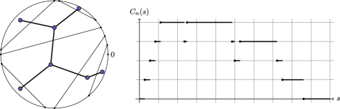
Figure 1: A lamination, its right-continuous height process and the corresponding rooted dual tree. Distances in the tree correspond to the number of chords separating fragments in the lamination.

Trees encoded by functions

Our main concern is the tree $T_{n}$ that is dual to the lamination $\mathfrak{L}_{n}$, and its scaling limit as $n\to\infty$. Each fragment in $\mathfrak{L}_{n}$ is associated with a node and two nodes $u$ and $v$ are connected in $T_{n}$ in the tree if and only if the corresponding fragments $S_{n}(u)$ and $S_{n}(v)$ share a chord $\ell$ of $\mathfrak{L}_{n}$ [more precisely $S_{n}(u)\cup S_{n}(v)\cup\ell$ is a connected component of $\mathscr{D}$]. Let $d_{n}$ be the graph distance in $T_{n}$, which comes with a natural distinguished point—the root—the fragment whose intersection with the circle $\mathscr{C}$ contains the point $0$. The encoding of laminations by functions turns out to also encode the dual tree. The value of the encoding function $C_{n}(s)$ at a given point $s\in[0,1]$ is precisely the height in $T_{n}$ (distance to the root) of the node corresponding to the face whose intersection with the circle contains the point $s$; see Figure 1. More precisely, the function $C_{n}$ actually encodes the metric structure of the dual tree $T_{n}$ in the following sense DuLe2005a , Aldous1993a , evans , LeGall2005 . Consider a càdlàg function $f\dvtx[0,1]\to[0,\infty)$ such that $f(0)=f(1)=0$ and $f(s)>0$ for all $s\in(0,1)$. Define $d_{f}:=[0,1]^{2}\to[0,\infty)$ by

$$d_{f}(x,y)=f(x)+f(y)-2\inf\bigl{\{}f(s)\dvtx x\wedge y\leq s\leq x\vee y\bigr{\}}.$$

One easily verifies that $d_{f}$ is a pseudo-metric on $[0,1]$. Let $x\sim y$ if $d_{f}(x,y)=0$. Write $\mathcal{T}_{f}$ for the quotient $[0,1]/\sim$ and consider the metric space $(\mathcal{T}_{f},d_{f})$. Then $(\mathcal{T}_{C_{n}},d_{C_{n}})$ is isometric to the dual tree $(T_{n},d_{n})$.

Real trees and Gromov–Hausdorff convergence

The natural scaling limits for large trees are real trees, which are encoded by continuous functions. A compact metric space $(X,d)$ is called a real tree if it is geodesic and acyclic:

• for every $x,y\in X$ there exists a unique isometry $\phi_{x,y}\dvtx[0,d(x,y)]\to X$ such that $\phi_{xy}(0)=x$ and $\phi_{xy}(d(x,y))=y$, and

• if $q$ is a continuous injective map from $[0,1]$ to $X$ such that $q(0)=x$ and $q(1)=y$ then $q([0,1])=\phi_{x,y}([0,d(x,y)])$.

For a càdlàg function $f$ with the properties above, the metric space $(\mathcal{T}_{f},d_{f})$ is a real tree.

Given two compact metric spaces $(X,d)$ and $(X^{\prime},d^{\prime})$, one defines the Gromov–Hausdorff distance $\mathrm{d_{\mathrm{GH}}}(X,X^{\prime})$ between $X$ and $X^{\prime}$ to be the infimum of all quantities $\delta_{\mathrm{H}}(\phi(X),\phi^{\prime}(X^{\prime}))$ ranging over the choice of compact metric spaces $(Z,\delta)$, and isometries $\phi\dvtx X\to Z$ and $\phi^{\prime}\dvtx X^{\prime}\to Z$, where $\delta_{\mathrm{H}}$ denotes the Hausdorff distance in $Z$. The distance $\mathrm{d_{\mathrm{GH}}}$ is a pseudo-metric between compact metric spaces, and induces a metric on the quotient space which identifies two metric spaces if they are isometric, see, for example, LeGall2005 , evans , Gromov1999 .

Comparing Hausdorff convergence of laminations and Gromov–Hausdorff convergence of their dual trees, the trees (or the height processes) are arguably the important objects: convergence of a sequence of increasing laminations as a subset of the complex plane only concerns the set of inserted chords, the time-scale and order in which they are inserted is completely irrelevant. Conversely, convergence of the (rescaled) height function implies convergence of the lamination under suitable mild additional assumptions; see Section 3.4.

1.2 Main results and general approach

Using the theory of fragmentation processes Bertoin2006 , Curien and Le Gall legalcu prove that there exists a random continuous process $\mathscr{M}$ which encodes the limiting triangulation in the sense that $\mathfrak{L}_{\infty}$ is distributed like $\mathfrak{L}_{\mathscr{M}}$. For this, they prove pointwise convergence of the encoding functions: for every $s\in[0,1]$, we have $n^{-\beta/2}C_{n}(s)\to\mathscr{M}(s)$ in probability, as $n\to\infty$, where the constant $\beta$ is given by

$$\beta=\frac{\sqrt{17}-3}{2}=0.561552\ldots.$$ (1)

They also show that for any $\varepsilon>0$, almost surely, the process $\mathscr{M}$ is $(\beta-\varepsilon)$-Hölder continuous and for any $s\in[0,1]$ we have

$$\mathbf{E}\bigl{[}\mathscr{M}(s)\bigr{]}=\kappa\bigl{(}s(1-s)\bigr{)}^{\beta}$$ (2)

for some constant $\kappa>0$ which was not identified in legalcu . Finally, the random function $\mathscr{M}$ inherits the recursive structure of the lamination process and satisfies the following distributional fixed-point equation: let $\mathscr{M}^{(0)},\mathscr{M}^{(1)}$ denote independent copies of $\mathscr{M}$, let also $(U,V)$ be independent of $(\mathscr{M}^{(0)},\mathscr{M}^{(1)})$ with density $2\mathbf{1}_{\{0\leq u\leq v\leq 1\}}$ on $[0,1]^{2}$. Then the process defined by

$$\qquad\cases{\displaystyle\bigl{(}1-(V-U)\bigr{)}^{\beta}\mathscr{M}^{(0)}\biggl{(}\frac{s}{1-(V-U)}\biggr{)},\qquad\mbox{if $s<U$},\vspace*{5pt}\cr\displaystyle\bigl{(}1-(V-U)\bigr{)}^{\beta}\mathscr{M}^{(0)}\biggl{(}\frac{U}{1-(V-U)}\biggr{)}+(V-U)^{\beta}\mathscr{M}^{(1)}\biggl{(}\frac{s-U}{V-U}\biggr{)},\vspace*{3pt}\cr\hskip 195.5pt\mbox{if $U\leq s<V$},\vspace*{5pt}\cr\displaystyle\bigl{(}1-(V-U)\bigr{)}^{\beta}\mathscr{M}^{(0)}\biggl{(}\frac{s-(V-U)}{1-(V-U)}\biggr{)},\qquad\mbox{if $s\geq V$,}}$$ (3)

is distributed like the initial process $\mathscr{M}$.

Note in passing that the constant $\beta$ defined in (1) appears in several contexts, such as the Hausdorff dimension of the standard random Cantor set, in the problem of parking arcs on the circle coffmall , bargne , in the analysis of the complexity of partial match retrieval algorithms in search trees FlPu1986 , FlGoPuRo1993 , cujo11 , BrNeSu12 or in models from biological physics phy . We prove that the convergence of $n^{-\beta/2}C_{n}$ to $\mathscr{M}$ is actually uniform with probability one. For any càdlàg or continuous function $f$, we denote its supremum by $\|f\|$.

Theorem 1.1

As $n\to\infty$, for the topology of uniform convergence on $[0,1]$,

$$n^{-\beta/2}C_{n}\to\mathscr{M}\qquad\mbox{almost surely and in }L^{m}\qquad\mbox{for all }m\in\mathbb{N}.$$ (4)

Up to a multiplicative constant, the process $\mathscr{M}$ is the unique solution of (3) (in distribution) with càdlàg paths subject to $\mathbf{E}[\|\mathscr{M}\|^{2}]<\infty$.

The theorem states $\|n^{-\beta/2}C_{n}-\mathscr{M}\|\to 0$ almost surely and in $L^{m}$ as $n\to\infty$. However, for technical reasons of measurability, the state space of càdlàg functions $\mathcal{D}[0,1]$ is endowed with the Skorokhod topology. We refer to the standard textbook by Billingsley bil68 for refined information on this matter.

Theorem 1.2

Almost surely as $n\to\infty$, we have

$$\bigl{(}\bigl{(}T_{n},n^{-\beta/2}d_{n}\bigr{)},\mathfrak{L}_{n}\bigr{)}\to\bigl{(}(\mathcal{T}_{\mathscr{M}},d_{\mathscr{M}}),\mathfrak{L}_{\mathscr{M}}\bigr{)}.$$

Here, the convergence of the components is with respect to the Gromov–Hausdorff distance between compact metric spaces and the Hausdorff metric on compact subsets of the disk $\mathscr{D}$.

The assertion about the convergence of the lamination is the main result in legalcu and we partially rely on their results to give a simplified proof using our approach. The convergence of the tree does not use any statement in legalcu , and proves the conjecture in Section 4.4 of legalcu . Note that the number of chords $N_{n}$ inserted by time $n$ is of order $\sqrt{n}$. More precisely, Curien and Le Gall legalcu show that $N_{n}/\sqrt{n}\rightarrow\sqrt{\pi}$ almost surely. So the volume of the tree $T_{n}$ is $N_{n}\sim(\pi n)^{1/2}$ and the order of magnitude of distances with respect to its volume is $N_{n}^{\beta}$.

In fact, it is not hard to see that $N_{n}$ is distributed like the number of maxima in a triangle when $n$ points are inserted uniformly at random and independent of each other. This quantity has been studied in detail by Bai et al. baihwang , who give exact formulas for the mean and the second moment together with first order expansions of all higher moments which imply asymptotic normality of $N_{n}$ after proper rescaling. We refer to Theorem 3 in baihwang for details.

The limit metric space $\mathcal{T}_{\mathscr{M}}$ is yet another natural random fractal real tree which does not come from a Brownian excursion Aldous1991a , Aldous1991b , Aldous1993a or another more general Lévy process LeLe1998 , DuLe2002 . Other examples include the fragmentation trees of Haas and Miermont HaMi2004a (see also HaMi12 ) and the minimum spanning tree of a complete graph whose scaling limit has been constructed by Addario-Berry et al. AdBrGoMi2012a .

A priori, the process $\mathscr{M}$ is not fully identified by the fixed-point equation (3) because of the free multiplicative constant. (Curien and Le Gall legalcu proved that the scaling constant $\kappa$ in (2) exists. They did not need to identify it for the main topic there is the limit lamination, which is not affected by this leading constant.) In order to identify $\mathscr{M}$ precisely, we study the asymptotics of $\mathbf{E}[C_{n}(\xi)]$ for an independent uniform random variable $\xi$. Let $\Gamma(s):=\int_{0}^{\infty}x^{s-1}e^{-x}\,dx$ denote the Gamma function.

Theorem 1.3

Let $\gamma=\beta/2+1$ and $\bar{\gamma}=\frac{-\sqrt{17}+1}{4}$. Then

$$\qquad\mathbf{E}\bigl{[}C_{n}(\xi)\bigr{]} = \frac{\sqrt{\pi}}{4}\sum_{k=1}^{n}\pmatrix{n\cr k}(-1)^{k+1}\frac{\Gamma(k-\gamma+1)\Gamma(k-\bar{\gamma}+1)}{k!\Gamma(k+3/2)\Gamma(2-\gamma)\Gamma(2-\bar{\gamma})}.$$ (5)

Furthermore, as $n\to\infty$,

$$\mathbf{E}\bigl{[}C_{n}(\xi)\bigr{]} = cn^{\beta/2}+O(1)$$

$$\eqntext{\displaystyle\mbox{with }c=\frac{\sqrt{\pi}\Gamma(2\gamma-1/2)}{2\Gamma(\gamma)\Gamma^{2}(\gamma+1/2)}=1.178226\ldots.}$$ (7)

The asymptotic expansion in (1.3) may be obtained from the work of Bertoin and Gnedin BeGn2004 on nonconservative fragmentations. More precisely, the first-order asymptotics is explicitly stated there, and the error term (that we need to prove the almost sure convergence in Theorems 1.1 and 1.2) follows from the same representation with a little more work. We include the explicit formula (5) since it seems that similar developments have attracted some interest in the community of analysis of algorithms ChHw2003 . Theorem 1.3 is not the heart of the matter here, but for the sake of completeness, we provide a proof in Appendix. Let $\mathrm{B}(x,y)=\int_{0}^{1}t^{x-1}(1-t)^{y-1}\,dt$ denote the beta function.

Corollary 1.4

The process $\mathscr{M}$ in (4) is such that

$$\mathbf{E}\bigl{[}\mathscr{M}(s)\bigr{]}=\kappa\bigl{(}s(1-s)\bigr{)}^{\beta},\qquad\kappa=\frac{c}{\mathrm{B}(\beta+1,\beta+1)}=3.34443\ldots,$$

where $c$ is given in (1.3), which identifies uniquely the solution of (3) among all processes with càdlàg paths subject to $\mathbf{E}[\|\mathscr{M}\|^{2}]<\infty$.

The homogeneous lamination

The lamination process we have introduced is actually an instance of a more general fragmentation process which is also discussed in legalcu , Section 2.4, using a two-stage split procedure: first pick a fragment with probability proportional to its mass to the power $\alpha$ (here $\alpha=2$), then choose the random chord within this fragment by sampling two independent uniform points on the intersection of the corresponding fragment with the circle. In the language of fragmentation theory Bertoin2006 , $\alpha$ is the index of self-similarity, and the actual split given the fragment is described by a dislocation measure, which is here (essentially) given by the two uniform points conditioned to fall in the same fragment. One may define related fragmentations where the next fragment to split is chosen with probability proportional to its mass to the power $\alpha\in\mathbb{R}$; the cases of interest here are those with $\alpha\geq 0$. When $\alpha\geq 0$, Curien and Le Gall legalcu , Section 2, have shown that the limit laminations are all identical. However, and although it encodes the same lamination for every $\alpha\geq 0$, the encoding process (related to the dual tree) depends on whether $\alpha>0$ or $\alpha=0$. The tree $(\mathcal{T}_{\mathscr{M}},d_{\mathscr{M}})$ is the scaling limit of the dual tree for every $\alpha>0$, but this raises the question of the dual tree in the case $\alpha=0$.

When $\alpha=0$, the choice of the next fragment is independent of its mass—hence homogeneous—and there is a drastic change in the behavior of the height process. At each step, the fragment containing the next chord is chosen uniformly at random. Note here that every trial yields a new insertion, and the lamination at time $n$ contains $n$ chords. Write $C_{n}^{h}(s)$ for the height in the dual tree of the fragment containing $s\in[0,1]$. Curien and Le Gall legalcu , Theorem 3.13, prove that for every $s\in(0,1)$ the quantity $n^{-1/3}C_{n}^{h}(s)$ converges almost surely as $n\to\infty$, where the pointwise limit $\mathscr{H}(s)$ may be described by a process $\mathscr{H}$ with continuous sample paths which satisfy another, similar but different, fixed-point equation (see Section 4).

In this case, the approach used to prove Theorem 1.2 yields the following result: let $T_{n}^{h}$ denote the tree dual to the homogeneous laminations $\mathfrak{L}_{n}^{h}$, and let $d_{n}^{h}$ denote the graph distance in $T_{n}^{h}$.

Theorem 1.5

Almost surely, as $n\to\infty$, we have

$$\bigl{(}\bigl{(}T_{n}^{h},n^{-1/3}d_{n}^{h}\bigr{)};\mathfrak{L}_{n}^{h}\bigr{)}\to\bigl{(}(\mathcal{T}_{\mathscr{H}},d_{\mathscr{H}});\mathfrak{L}_{\mathscr{H}}\bigr{)}.$$

The convergence of the dual tree is with respect to Gromov–Hausdorff topology, and the lamination converges for the Hausdorff topology on compact subsets of the disk.

The second assertion of the Theorem 1.5 has been proved in legalcu , and our contribution relies in the proof of convergence of the dual tree. Our approach to Theorem 1.5 relies on the same functional ideas developed for the self-similar case and the proof of Theorem 1.2. We explain them below in more detail.

As already indicated, we have $\mathfrak{L}_{\mathscr{M}}=\mathfrak{L}_{\mathscr{H}}$ almost surely. In terms of the dual trees, this corresponds to the fact that the equivalence relations given by $d_{\mathscr{M}}$ and $d_{\mathscr{H}}$ almost surely identify the same points on the unit interval. This highlights the difference between convergence in the Hausdorff distance solely relying on $\mathcal{T}_{\mathscr{M}}=\mathcal{T}_{\mathscr{H}}$ as collection of equivalence classes of $[0,1]$, not involving the geometry of the limit objects and convergence of the dual trees to $(\mathcal{T}_{\mathscr{M}},d_{\mathscr{M}})$ [and $(\mathcal{T}_{\mathscr{H}},d_{\mathscr{H}})$, resp.] seen as metric spaces.

About the main ideas

The main techniques in legalcu are inherently pointwise, and one of the main difference in spirit in our approach is to consider the problem as functional from the very beginning. In particular, we develop a new construction for the limit process $\mathscr{M}$. We construct the random process $Z$ (which is almost surely equal to $\mathscr{M}$) as the uniform limit of continuous functions $Z_{n}\dvtx[0,1]\to[0,\infty)$ which are designed so that $(Z_{n}(s),n\geq 0)$ is a nonnegative martingale for every $s\in[0,1]$. Unlike in legalcu where results entirely rely on an approach that is forward in time, we make use of the inherent recursive structure of the problem and study the telescoping sum representation

$$Z_{n}-Z_{0}=\sum_{i=0}^{n-1}(Z_{i+1}-Z_{i}).$$

More precisely, this backward approach is based on an $L^{2}$ argument using the fact that one can bound $\|Z_{i+1}-Z_{i}\|^{2}$ in terms of independent copies of $\|Z_{i}-Z_{i-1}\|$ corresponding to the two fragments created by the insertion of the first chord as in (3). The expansion of the square yields one contribution involving the single fragment ($\mathbf{E}[\|Z_{i}-Z_{i}\|^{2}]$) and one involving the first two fragments, which may be bounded using only $\mathbf{E}[|Z_{i}(\xi)-Z_{i-1}(\xi)|^{2}]$ for a uniform random variable $\xi$. So our representation allows to leverage the convergence at a uniformly distributed random point (Lemma 2.2) to deduce $\mathbf{E}[\|Z_{i+1}-Z_{i}\|^{2}]\leq\chi\cdot\mathbf{E}[\|Z_{i}-Z_{i-1}\|^{2}]$ for some $\chi<1$ and all $i$ sufficiently large leading to geometric convergence in a functional sense. The convergence of the discrete sequence $n^{-\beta/2}C_{n}$ is obtained in a similar vein. After using an appropriate embedding of both the sequence and the limit $Z$, our backward approach technically relies on ideas from the contraction method Ro91 , RaRu95 , NeRu04 ; see also NeSu12 for a recent development in function spaces. A somewhat similar approach toward functional convergence results relying on first establishing one-dimensional convergence at a specific point in the context of the Quicksort algorithm can be found in Ragab and Rösler ragabroe .

1.3 Related work on random laminations of the disk

The work of Curien and Le Gall legalcu was motivated by the pioneering work of Aldous al94circle , al94 who studied uniform random triangulations of the disk which arise as limiting objects for uniform triangulations of regular $n$-gons as $n\to\infty$. In the case of uniform random triangulations, the process which encodes the limit triangulation is the Brownian excursion, and the scaling limit of the sequence of dual trees is the Brownian continuum random tree introduced in Aldous1991a , Aldous1991b , Aldous1993a .

Among the recent work on laminations of the disk, one can mention CuKo2012a where Curien and Kortchemski showed that the Brownian triangulation is also the scaling limit of other random subsets of the disk, in particular, noncrossing trees (sets of noncrossing chords which form a tree) MaPa2002 , and dissections (noncrossing sets of chords) under the uniform distribution. By sampling tessellations according to a Boltzmann weight depending on the degree of the faces, Kortchemski Ko2011b obtained limit laminations which are not triangulations and are encoded by excursions of stable spectrally positive Lévy processes (with Lévy measure concentrated on $[0,\infty)$). Finally, Curien and Werner CuWe2011a have studied geodesic laminations of the Poincaré disk. They construct and study the unique random tiling of the hyperbolic plane into triangles with vertices on the boundary whose distribution is invariant under Möbius transformations and satisfies a certain spatial Markov property.

Plan of the paper

In Section 2, we give our construction of a continuous solution $Z$ of (3) with $\mathbf{E}[Z(s)]=\kappa(s(1-s))^{\beta}$. (Recall that $Z=\mathscr{M}$ almost surely.) The construction guarantees finiteness of all moments of the supremum $\|Z\|$ which is essential for our approach. Here, we also prove the characterization of $Z$ as a solution of (3) under additional conditions. In Section 3, we prove the uniform convergence of $n^{-\beta/2}C_{n}$ to $Z$. We also obtain an upper bound on the rate of convergence in the $L^{m}$ distance, $m\geq 1$, which yields the almost sure convergence in Theorem 1.1. Here, we also show how our results simplify the arguments to deduce convergence of the lamination. Section 4 is devoted to the proof of Theorem 4.1 which covers the homogeneous case $\alpha=0$. Finally, in Section 5 we prove some properties about the dual tree $\mathcal{T}_{Z}=\mathcal{T}_{\mathscr{M}}$, in particular about its fractal dimension. Our proof of Theorem 1.3 is based on generating functions and is given in Appendix to keep the body of the paper more focused.

2 A functional construction of the self-similar limit height process

Our aim in this section is to propose an alternative construction of the limit process $Z$. Although Curien and Le Gall legalcu have proved the existence of a continuous process $\mathscr{M}$ (which is almost surely equal to $Z$) using bounds on the moments on the increments and Kolmogorov’s criterion ReYo1991 , Theorem 2.1, we adopt here a functional approach that will later guide our proof of the convergence theorem (Theorem 1.1).

The process $Z$ is constructed in terms of a set of independent random variables on the unit interval as follows. First, we identify the nodes of the infinite binary tree with the set of finite words on the alphabet $\{0,1\}$,

$$\mathcal{T}=\bigcup_{n\geq 0}\{0,1\}^{n}.$$

The descendants of $u\in\mathcal{T}$ correspond to all the words in $\mathcal{T}$ with prefix $u$. Let $\{(U_{v},V_{v}),v\in\mathcal{T}\}$ be a set of independent and identically distributed two-dimensional random vectors with density $2\mathbf{1}_{\{0\leq u\leq v\leq 1\}}$ and $A^{+}=\{(u,v)\in[0,1]^{2}\dvtx u<v\}$. For convenience, we also set $U:=U_{\varnothing}$ and $V:=V_{\varnothing}$ and define

$$h(s)=\bigl{(}s(1-s)\bigr{)}^{\beta}.$$

Let $\mathcal{C}_{0}([0,1])$ denote the set of continuous functions $f$ on the unit interval vanishing at the boundary, that is, $f(0)=f(1)=0$. Define the operator $G\dvtx A^{+}\times\mathcal{C}_{0}([0,1])^{2}\to\mathcal{C}_{0}([0,1])$ by

$$G[u,v;f_{0},f_{1}](s)=\cases{\displaystyle\bigl{(}1-(v-u)\bigr{)}^{\beta}f_{0}\biggl{(}\frac{s}{1-(v-u)}\biggr{)},\qquad\mbox{if $s<U$},\vspace*{5pt}\cr\displaystyle\bigl{(}1-(v-u)\bigr{)}^{\beta}f_{0}\biggl{(}\frac{u}{1-(v-u)}\biggr{)}+(v-u)^{\beta}f_{1}\biggl{(}\frac{s-u}{v-u}\biggr{)},\vspace*{3pt}\cr\hskip 170.0pt\mbox{if $U\leq s<V$,}\vspace*{5pt}\cr\displaystyle\bigl{(}1-(v-u)\bigr{)}^{\beta}f_{0}\biggl{(}\frac{s-(v-u)}{1-(v-u)}\biggr{)},\qquad\mbox{if $s\geq V$.}}$$

For convenience, define

$$K_{0}(s;u,v) = \mathbf{1}_{\{s<u\}}\frac{s}{1-(v-u)}+\mathbf{1}_{\{s\geq v\}}\frac{s-(v-u)}{1-(v-u)}$$ (8)

$${}+\mathbf{1}_{\{u\leq s<v\}}\frac{u}{1-(v-u)},$$

$$K_{1}(s;u,v) = \mathbf{1}_{\{u\leq s<v\}}\frac{s-u}{v-u},$$

so that we have the more compact form

$$G[u,v;f_{1},f_{2}](s)=\bigl{(}1-(v-u)\bigr{)}^{\beta}f_{0}\bigl{(}K_{0}(s;u,v)\bigr{)}+(v-u)^{\beta}f_{1}\bigl{(}K_{1}(s;u,v)\bigr{)}.$$

For every node $u\in\mathcal{T}$, let $Z_{0}^{(u)}=\kappa h(s)$. Then define recursively

$$Z_{n+1}^{(u)}=G\bigl{(}U_{u},V_{u};Z_{n}^{(u0)},Z_{n}^{(u1)}\bigr{)},$$ (9)

and define $Z_{n}=Z_{n}^{\varnothing}$ to be the value observed at the root of $\mathcal{T}$. For every $s\in(0,1)$, one can verify that the sequence $(Z_{n}(s),n\geq 0)$ is a nonnegative martingale for the filtration $\mathcal{F}_{n}=\sigma((U_{u},V_{u})\dvtx|u|\leq n)$, so that $Z_{n}(s)$ converges almost surely. (This reduces to proving that $\mathbf{E}[G(U,V;h,h)(s)]=h(s)$ for every $s\in[0,1]$, and is essentially proved in the first moment calculation in Section 4.2 of legalcu .) The game is now to prove that this convergence is actually uniform for $s\in(0,1)$, which will yield the following theorem. (See Figure 2 for a simulation.)

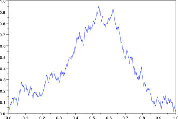
Figure 2: An instance of limit height process $Z/\kappa$ simulated using the approximations $Z_{n}/\kappa,n\geq 1$.

Theorem 2.1

For any $u\in\mathcal{T}$, almost surely, the sequence $Z_{n}^{(u)}$ converges uniformly to a continuous process $Z^{(u)}$. Almost surely, for every $s\in[0,1]$, we have

$$Z(s)=\cases{\displaystyle\bigl{(}1-(V-U)\bigr{)}^{\beta}Z^{(0)}\biggl{(}\frac{s}{1-(V-U)}\biggr{)},\qquad\mbox{if $s<U$,}\vspace*{5pt}\cr\displaystyle\bigl{(}1-(V-U)\bigr{)}^{\beta}Z^{(0)}\biggl{(}\frac{U}{1-(V-U)}\biggr{)}+(V-U)^{\beta}Z^{(1)}\biggl{(}\frac{s-U}{V-U}\biggr{)},\vspace*{3pt}\cr\hskip 190.0pt\mbox{if $U\leq s<V$,}\vspace*{5pt}\cr\displaystyle\bigl{(}1-(V-U)\bigr{)}^{\beta}Z^{(0)}\biggl{(}\frac{s-(V-U)}{1-(V-U)}\biggr{)},\qquad\mbox{if $s\geq V$.}}$$ (10)

Moreover, $\mathbf{E}[\|Z\|^{m}]<\infty$ for all $m\in\mathbb{N}$, $\mathbf{E}[Z(s)]=\kappa h(s)$ and writing $\mathcal{L}(X)$ for the law of $X$, we have $\mathcal{L}(Z^{(u)})=\mathcal{L}(Z)$ for all $u\in\mathcal{T}$.

From the theorem above and its proof given subsequently, one deduces that the random variable $Y=Z(\xi)$ where $\xi$ is an independent uniformly distributed random variable satisfies the following distribution fixed-point equation:

$$Y\stackrel{{\scriptstyle d}}{{=}}\bigl{(}1-(V-U)\bigr{)}^{\beta}Y+\mathbf{1}_{\{U\leq\xi<V\}}(V-U)^{\beta}\widehat{Y}.$$ (11)

Here, $\widehat{Y}$ is distributed as $Y$ and the random variables $Y$, $\widehat{Y}$, $\xi$, and $(U,V)$ are independent. In fact, this identity is at the very heart of the proof of Theorem 2.1 as will become clear below.

Note that any set of independent vectors $(U_{v},V_{v})_{v\in\mathcal{T}}$ with distribution $2\mathbf{1}_{\{0<u<v<1\}}$ can be used in the construction given in this section. It is in the next section where we make a specific choice of the set in order to couple the limit to the discrete lamination process. In sodawir , BrNeSu12 , a similar construction has been used in a related context: there, the uniform convergence follows from a bootstrap of the pointwise convergence which requires tedious verifications. Here, we prove directly that the convergence is uniform using an $L^{2}$ argument.

Write $\Psi=U/(1-(V-U))$. By the definition of $Z_{n}$, we have the following expansion:

$$\bigl{[}Z_{n+1}(s)-Z_{n}(s)\bigr{]}^{2}$$

$$\qquad=\bigl{(}1-(V-U)\bigr{)}^{2\beta}\bigl{[}Z_{n}^{(0)}\bigl{(}K_{0}(s;U,V)\bigr{)}-Z_{n-1}^{(0)}\bigl{(}K_{0}(s;U,V)\bigr{)}\bigr{]}^{2}$$

$$\quad\qquad{}+\mathbf{1}_{\{U\leq s<V\}}(V-U)^{2\beta}\bigl{[}Z_{n}^{(1)}\bigl{(}K_{1}(s;U,V)\bigr{)}-Z_{n-1}^{(1)}\bigl{(}K_{1}(s;U,V)\bigr{)}\bigr{]}^{2}$$

$$\quad\qquad{}+\mathbf{1}_{\{U\leq s<V\}}2\bigl{(}(V-U)\bigl{(}1-(V-U)\bigr{)}\bigr{)}^{\beta}\bigl{[}Z_{n}^{(0)}(\Psi)-Z_{n-1}^{(0)}(\Psi)\bigr{]}$$

$$\qquad\qquad{}\times\bigl{[}Z_{n}^{(1)}\bigl{(}K_{1}(s;U,V)\bigr{)}-Z_{n-1}^{(1)}\bigl{(}K_{1}(s;U,V)\bigr{)}\bigr{]}.$$

Define

$$q = \mathbf{E}\bigl{[}\bigl{(}1-(V-U)\bigr{)}^{2\beta}\bigr{]}+\mathbf{E}\bigl{[}(V-U)^{2\beta}\bigr{]}$$ (13)

$$= \frac{2}{2\beta+1}=\frac{2}{\sqrt{17}-2}<1,$$

$$q^{\prime} = 2\sqrt{\mathbf{E}\bigl{[}\bigl{(}(V-U)\bigl{(}1-(V-U)\bigr{)}\bigr{)}^{2\beta}\bigr{]}}.$$

Then equation (2) yields

$$\mathbf{E}\bigl{[}\|Z_{n+1}-Z_{n}\|^{2}\bigr{]}$$

$$\qquad\leq q\mathbf{E}\bigl{[}\|Z_{n}-Z_{n-1}\|^{2}\bigr{]}$$

$$\quad\qquad{}+2\mathbf{E}\bigl{[}\bigl{(}(V-U)\bigl{(}1-(V-U)\bigr{)}\bigr{)}^{\beta}$$

(14)

$$\hskip 60.0pt{}\times\bigl{|}Z_{n}^{(0)}(\Psi)-Z_{n-1}^{(0)}(\Psi)\bigr{|}\cdot\bigl{\|}Z_{n}^{(1)}-Z_{n-1}^{(1)}\bigr{\|}\bigr{]}$$

$$\qquad\leq q\mathbf{E}\bigl{[}\|Z_{n}-Z_{n-1}\|^{2}\bigr{]}$$

$$\quad\qquad{}+q^{\prime}\sqrt{\mathbf{E}\bigl{[}\|Z_{n}-Z_{n-1}\|^{2}\bigr{]}\cdot\mathbf{E}\bigl{[}\bigl{(}Z_{n}^{(0)}(\Psi)-Z_{n-1}^{(0)}(\Psi)\bigr{)}^{2}\bigr{]}}$$

by the Cauchy–Schwarz inequality. If we were to drop the second term in the last line above, we would have geometric convergence of $\mathbf{E}[\|Z_{n+1}-Z_{n}\|^{2}]$ since $q<1$. Now, the crucial observation is that, the second term may actually be shown to decrease geometrically using only the convergence at a uniformly random point. More precisely, the random variable $\Psi$ is uniform on $[0,1]$ and independent of $\{(U_{v},V_{v})\dvtx v\in\mathcal{T}_{0}\}$, where $\mathcal{T}_{0}=\{0u\dvtx u\in\mathcal{T}\}$. Thus,

$$Z_{n}^{(0)}(\Psi)-Z_{n-1}^{(0)}(\Psi)\stackrel{{\scriptstyle d}}{{=}}Z_{n}(\xi)-Z_{n-1}(\xi),$$

where $\xi$ is uniformly distributed on the unit interval and independent of $\{(U_{v},V_{v})\dvtx v\in\mathcal{T}\}$. The following lemma allows to bound the second summand in (2).

Lemma 2.2

There exists a constant $C_{1}>0$ such that, for all natural number $n\geq 1$,

$$\mathbf{E}\bigl{[}\bigl{(}Z_{n}(\xi)-Z_{n-1}(\xi)\bigr{)}^{2}\bigr{]}\leq C_{1}^{2}q^{n}.$$

For the sake of clarity, we take Lemma 2.2 for granted for now and show that it indeed implies exponential bounds for $\mathbf{E}[\|Z_{n+1}-Z_{n}\|^{2}]$.

Lemma 2.3

For any $0<\eta<1-q^{1/2}$, there exists a constant $C_{2}$ such that for all $n\geq 0$,

$$\mathbf{E}\bigl{[}\|Z_{n+1}-Z_{n}\|^{2}\bigr{]}\leq C_{2}\bigl{(}q^{1/2}+\eta\bigr{)}^{n}.$$

Write $\Delta_{n}=\mathbf{E}[\|Z_{n+1}-Z_{n}\|^{2}]$ for $n\geq 0$. Then the inequalities (2) and Lemma 2.2 yield, for every natural number $n$,

$$\Delta_{n}\leq q\Delta_{n-1}+C_{1}q^{\prime}q^{n/2}\Delta_{n-1}^{1/2}.$$ (15)

First, (15) clearly implies that $\Delta_{n}$ is bounded: we have

$$\Delta_{n}\leq\bigl{(}q+C_{1}q^{\prime}q^{n/2}\bigr{)}\cdot\max\{\Delta_{i}\vee 1\dvtx 0\leq i<n\}.$$

So, taking $n_{0}$ large enough that $q+C_{1}q^{\prime}q^{n/2}<1$ for all $n\geq n_{0}$, it follows that for all $n\geq n_{0}$, we have $\Delta_{n}\leq\max\{\Delta_{i},i\leq n_{0}\}\vee 1$.

Now, fix $0<\eta<1-q^{1/2}$ and $M$ such that $\Delta_{n}\leq M^{2}$ for all $n\in\mathbb{N}_{0}$. Let $n_{1}$ be large enough such that for any $n\geq n_{1}$, we have

$$\frac{MC_{1}q^{\prime}}{q^{1/2}+\eta}\biggl{(}\frac{q^{1/2}}{q^{1/2}+\eta}\biggr{)}^{n}\leq 1.$$

We now proceed by induction on $n\geq n_{1}$. Assume that $\Delta_{n}\leq C_{2}(q^{1/2}+\eta)^{n}$ for $n\leq n_{1}$ where the constant $C_{2}$ is chosen large enough such that $qC_{2}\leq(C_{2}-1)(q^{1/2}+\eta)$. Then by (15), we have

$$\Delta_{n+1} \leq qC_{2}\bigl{(}q^{1/2}+\eta\bigr{)}^{n}+MC_{1}q^{\prime}q^{n/2}$$

$$\leq \bigl{(}q^{1/2}+\eta\bigr{)}^{n+1}\biggl{[}\frac{C_{2}q}{q^{1/2}+\eta}+\frac{MC_{1}q^{\prime}}{q^{1/2}+\eta}\biggl{(}\frac{q^{1/2}}{q^{1/2}+\eta}\biggr{)}^{n}\biggr{]}$$

$$\leq C_{2}\bigl{(}q^{1/2}+\eta\bigr{)}^{n+1}$$

by our choice for $C_{2}$ and $n_{1}$, which completes the proof.

With Lemma 2.3 in hand, we may now complete the proof of Theorem 2.1. Proof of Theorem 2.1 The fact that there exists a continuous process $Z$ such that $Z_{n}\to Z$ uniformly almost surely follows from standard arguments: first, Markov’s inequality, monotone convergence and the Cauchy–Schwarz inequality imply that $\sup_{m\geq n}\|Z_{m}-Z_{n}\|\to 0$ in probability. It easily follows that also $\sup_{m,p\geq n}\|Z_{m}-Z_{p}\|\to 0$ in probability. By monotonicity, the latter convergence is actually almost sure. Thus, the sequence $(Z_{n},n\geq 0)$ is almost surely uniformly Cauchy. Since $Z_{n}$ is continuous for every $n\geq 0$, the completeness of $\mathcal{C}[0,1]$ implies the existence of a limit function $Z$ which is almost surely continuous.

The sequences $Z_{n}^{(0)}$ and $Z_{n}^{(1)}$, $n\geq 1$, also converge since they are both distributed like $Z_{n-1}$, $n\geq 1$. Write $Z^{(0)}$ and $Z^{(1)}$ their uniform almost sure limits. Letting $n\rightarrow\infty$, in the definition of $Z_{n}$ in (9) implies the equality in (10).

Next, we prove that $\sup_{n\geq 1}\mathbf{E}[\|Z_{n}\|^{m}]<\infty$ for any $m\in\mathbb{N}$ by induction on $m$. It is true for $m=1,2$ and we assume it holds for any $\ell<m$ with $m>2$. Then, by construction

$$\mathbf{E}\bigl{[}\|Z_{n}\|^{m}\bigr{]} \leq \underbrace{\bigl{(}\mathbf{E}\bigl{[}\bigl{(}1-(V-U)\bigr{)}^{m\beta}\bigr{]}+\mathbf{E}\bigl{[}(V-U)^{m\beta}\bigr{]}\bigr{)}}_{q_{m}}\cdot\mathbf{E}\bigl{[}\|Z_{n-1}\|^{m}\bigr{]}$$

$${}+\sum_{i=1}^{m-1}\pmatrix{m\cr i}\mathbf{E}\bigl{[}\|Z_{n-1}\|^{i}\bigr{]}\mathbf{E}\bigl{[}\|Z_{n-1}\|^{m-i}\bigr{]}.$$

The induction hypothesis implies that the summand in (2) is bounded uniformly in $n$. Since $q_{m}<1$, an easy induction on $n$ gives the desired result $\sup_{n\geq 1}\mathbf{E}[\|Z_{n}\|^{m}]<\infty$. It follows that $\mathbf{E}[\|Z\|^{m}]<\infty$ for any $m\in\mathbb{N}$.

Finally, the fact that $\mathbf{E}[Z_{n}(s)]=\kappa h(s)$ for all $n$, and thus $\mathbf{E}[Z(s)]=\kappa h(s)$, is essentially equivalent to the martingale property of $Z_{n}(s)$ mentioned above and can be found in legalcu , Section 4.2. This completes the proof.

It now remains to prove Lemma 2.2 about the bound on $\mathbf{E}[|Z_{n}(\xi)-Z_{n-1}(\xi)|^{2}]$. Proof of Lemma 2.2 Let $W_{0}=K_{0}(\xi,U,V)$ and $W_{1}=K_{1}(\xi,U,V)$. The key ingredient of the proof is the following observation:

1. [(O1)]

2. On the event $\{\xi\notin(U,V]\}$, the quantities $W_{0}$ and $V-U$ are independent and $W_{0}$ has uniform distribution. Moreover, given the event $\{U\leq\xi<V\}$, the quantities $W_{0}$, $W_{1}$ and $V-U$ are independent and both $W_{0}$ and $W_{1}$ have uniform distribution.

Using this observation in (2) directly implies the desired result

$$\mathbf{E}\bigl{[}\bigl{|}Z_{n+1}(\xi)-Z_{n}(\xi)\bigr{|}^{2}\bigr{]}\leq q\mathbf{E}\bigl{[}\bigl{|}Z_{n}(\xi)-Z_{n-1}(\xi)\bigr{|}^{2}\bigr{]},$$

since the mixed terms cancel out for the expected value $\mathbf{E}[Z_{n}^{(u)}(\xi)]=\kappa\mathrm{B}(\beta+1,\beta+1)$ is independent of $u\in\mathcal{T}$ and $n\geq 0$. To complete this section, we show that the process $Z$ we have constructed is characterized by the fixed-point equation (10) in a reasonable class of processes.

Proposition 2.4

The process $Z$ is the unique solution of the fixed-point equation (3) (in distribution) among all càdlàg processes subject to $\mathbf{E}[Z(\xi)]=\kappa\mathrm{B}(\beta+1,\beta+1)$ and $\mathbf{E}[\|Z\|^{2}]<\infty$.

The main part of the proof relies on the functional contraction method developed in NeSu12 . Let $\mathcal{M}(\mathcal{D}[0,1])$ denote the set of probability measures on $\mathcal{D}[0,1]$. Consider the map $T\dvtx\mathcal{M}(\mathcal{D}[0,1])\to\mathcal{M}(\mathcal{D}[0,1])$ which to $\mu\in\mathcal{M}(\mathcal{D}[0,1])$ assigns the law of the process

$$\bigl{(}1-(V-U)^{\beta}\bigr{)}X\bigl{(}K_{0}(s;U,V)\bigr{)}+(V-U)^{\beta}\widehat{X}\bigl{(}K_{1}(s;U,V)\bigr{)},$$

where $X,\widehat{X}$ are independent functions sampled according to $\mu$, both independent of $(U,V)$. Let $\mathcal{M}_{2}(h)\subseteq\mathcal{M}(\mathcal{D}[0,1])$ be the subset of measures $\mu$ such that if $X$ is $\mu$-distributed then $\mathbf{E}[\|X\|^{2}]<\infty$ and $\mathbf{E}[X(t)]=h(t)$ for all $t\in[0,1]$. Lemma 18 in NeSu12 asserts that $T$ is contractive with respect to the Zolotarev metric $\zeta_{2}$ in the space $\mathcal{M}_{2}(h)$ where the Lipschitz constant can be chosen as $q<1$ given in (13). This lemma relies on a discrete sequence [denoted $(X_{n})$ there] satisfying conditions (C1), (C2), (C3) formulated on page 20 in NeSu12 . In our setting, as we deal directly with the limiting fixed-point equation, conditions (C1) and (C3) reduce to the fact that $T(\mathcal{M}_{2}(h))\subseteq\mathcal{M}_{2}(h)$. This can be shown by a direct computation (see, e.g., legalcu , Section 4.2). Condition (C2) is satisfied for we have $q=\mathbf{E}[(1-(V-U))^{2\beta}]+\mathbf{E}[(V-U)^{2\beta}]<1$. Furthermore, Curien and Le Gall legalcu , Section 4.2, prove that the mean function of any solution $X$ of (3) with $\int_{0}^{1}\mathbf{E}[|X(s)|]<\infty$ is a multiple of $h$. This completes the proof.

3 Convergence of the discrete process

3.1 Notation and setting

Let $(U_{i}^{\prime},V_{i}^{\prime})_{i\geq 1}$ be a sequence of independent vectors, where for each $i\geq 1$, $U_{i}^{\prime},V_{i}^{\prime}$ are independent and have uniform distribution on the unit interval. We consider the lamination process built from this set of vectors as explained in the Introduction. Let us first explain the connection with the tree-based construction of Section 2. It should be intuitively clear how the family $(U_{v},V_{v})_{v\in\mathcal{T}}$ used to build the limit is constructed from $(U_{i}^{\prime},V_{i}^{\prime})_{i\geq 1}$; the precise statement requires additional notation.

Initially, there is a single fragment $S^{\varnothing}$ consisting of the entire disk $\mathscr{D}$, which is associated to the root $\varnothing\in\mathcal{T}$. For $n=1$, $U_{1}^{\prime}$ and $V_{1}^{\prime}$ of course both fall inside the unique fragment and we insert the chord connecting $U_{1}^{\prime}$ and $V_{1}^{\prime}$. This chord divides $S^{(\varnothing)}$ into two fragments $S^{(0)}$, $S^{(1)}$, where $S^{(0)}$ denotes the fragment containing $0$. Define

$$U:=U_{\varnothing}=\min\bigl{(}U_{1}^{\prime},V_{1}^{\prime}\bigr{)}\quad\mbox{and}\quad V:=V_{\varnothing}=\max\bigl{(}U_{1}^{\prime},V_{1}^{\prime}\bigr{)}.$$

In general, at some stage $n-1$, $n>1$, of the process, we have inserted some chords, and associated fragments to the nodes in a finite subtree $T_{n-1}$ of $\mathcal{T}$ (a connected set containing the root). Then, at step time $n>1$, if there is no node $u\in T_{n}$ such that one of $U_{n}^{\prime},V_{n}^{\prime}$ falls inside $S^{(u)}$ and the other outside (i.e., the chord connecting $U_{n}^{\prime}$ and $V_{n}^{\prime}$ does not intersect any other previously inserted chord), we insert the chord connecting them. Let $S^{(v)}$ be the smallest fragment containing both $U_{n}^{\prime}$ and $V_{n}^{\prime}$; the chord joining $U_{n}^{\prime}$ to $V_{n}^{\prime}$ splits $S^{(v)}$ into two fragments $S^{(v0)}$ and $S^{(v1)}$; the labeling is chosen such that $v0$ is closer to the root in the dual tree. Moreover, writing $\operatorname{Leb}$ for Lebesgue measure on the circle $\mathscr{C}$, we let

$$\ell^{(v)}=\operatorname{Leb}\bigl{(}S^{(v)}\cap\mathscr{C}\bigr{)}$$ (17)

be the mass of the fragment $S^{(v)}$, and

$$U_{v} = \frac{\min(U_{n}^{\prime},V_{n}^{\prime})-\operatorname{Leb}(\{s\notin S^{(v)}\cap\mathscr{C}\dvtx 0<s\leq\min(U_{n}^{\prime},V_{n}^{\prime})\})}{\ell^{(v)}},$$

$$V_{v} = \frac{\max(U_{n}^{\prime},V_{n}^{\prime})-\operatorname{Leb}(\{s\notin S^{(v)}\cap\mathscr{C}\dvtx 0<s\leq\max(U_{n}^{\prime},V_{n}^{\prime})\})}{\ell^{(v)}}.$$

Then $(U_{v},V_{v})_{v\in\mathcal{T}}$ is a set of independent random vectors each having density $2\mathbf{1}_{\{0<u<v<1\}}$. In the following, for any $u\in\mathcal{T}$, $Z^{(u)}$ will denote the process constructed in Section 2 using this set of vectors.

For any $n\in\mathbb{N}$, let $\tau_{0}(n)$ be the first time $k$ when there exist exactly $n$ integers $2\leq\ell_{1}<\cdots<\ell_{n}=k$ such that $U_{\ell_{i}}^{\prime},V_{\ell_{i}}^{\prime}$, $i=1,\ldots,n$, both take values in $S^{(0)}$ (actually $S^{(0)}\cap\mathscr{C}$). Analogously, let $\tau_{1}(n)$ be defined in the same way using the segment $S^{(1)}$. Observe that $\tau_{0}(n)$ and $\tau_{1}(n)$ are only the stopping times when $n$ trials have been made in $S^{(0)}$ and $S^{(1)}$, respectively, and that these trials may not have all led to the successful insertion of a chord. For $n\in\mathbb{N}$, let $C_{n}^{(0)}(s)$ be the number of chords intersecting the straight line going from $0$ to $\varphi_{0}(s)$ defined by

$$\varphi_{0}(s)=s\bigl{(}1-(V-U)\bigr{)}+(V-U)\mathbf{1}_{\{s>\Psi\}}$$

at time $\tau_{0}(n)$. Here and for the remainder of this section, we use $\Psi:=U/(1+U-V)$ as in Section 2. Note that $\varphi_{0}(s)$ is the natural parameterization for $C_{n}^{(0)}$ in the sense that $(C_{n}^{(0)})_{n\geq 0}$ has the same distribution as $(C_{n})_{n\geq 0}$. Observe that $C_{n}^{(0)}$ is well defined since $\tau_{0}(n)<\infty$ almost surely for all $n\in\mathbb{N}$. Analogously, let $C_{n}^{(1)}(s)$ be the number of chords intersecting the straight line going from $U$ to $\varphi_{1}(s)$ where

$$\varphi_{1}(s)=s(V-U)+U$$

at the stopping time $\tau_{1}(n)$. For convenience, let $C_{0}^{(0)}=C_{0}^{(1)}\equiv 0$. At time $n$, let $I^{(0)}_{n}$ and $I^{(1)}_{n}$ be the number of pairs among $(U_{i}^{\prime},V_{i}^{\prime})$, $i=2,\ldots,n$, whose components both fall in $S^{(0)}$ and $S^{(1)}$, respectively. Finally, let $F_{n}=n-1-I^{(0)}_{n}-I^{(1)}_{n}$ be the number of failures, or unsuccessful insertion attempts by time $n$ due to one point falling in $S^{(0)}$ and the other in $S^{(1)}$. Then, given the first chord $(U,V)$,

$$\mathcal{L}\bigl{(}I^{(0)}_{n},I^{(1)}_{n},F_{n}\bigr{)}$$

$$\qquad=\operatorname{Multi}\bigl{(}n-1;\bigl{(}1-(V-U)\bigr{)}^{2},(V-U)^{2},2(V-U)\bigl{(}1-(V-U)\bigr{)}\bigr{)}.$$

Almost surely, for every $s\in[0,1]$, we have

$$C_{n}(s)=\cases{\displaystyle C^{(0)}_{I^{(0)}_{n}}\biggl{(}\frac{s}{1-(V-U)}\biggr{)},\qquad\mbox{if $s<U$,}\vspace*{5pt}\cr\displaystyle C^{(0)}_{I^{(0)}_{n}}\biggl{(}\frac{U}{1-(V-U)}\biggr{)}+1+C^{(1)}_{I^{(1)}_{n}}\biggl{(}\frac{s-U}{V-U}\biggr{)},\vspace*{3pt}\cr\hskip 121.5pt\mbox{if $U\leq s<V$,}\vspace*{5pt}\cr\displaystyle C^{(0)}_{I^{(0)}_{n}}\biggl{(}\frac{s-(V-U)}{1-(V-U)}\biggr{)},\qquad\mbox{if $s\geq V$.}}$$ (18)

Let $\xi$ be a uniform random variable, independent of $(U_{i}^{\prime},V_{i}^{\prime})_{i\geq 1}$. Then, we let $X_{n}$ be the following rescaled version of $C_{n}$, for any $n\geq 1$:

$$X_{n}(s):=C_{n}(s)\frac{\kappa\mathrm{B}(\beta+1,\beta+1)}{\mathbf{E}[C_{n}(\xi)]}.$$

3.2 Uniform convergence in $L^{2}$

The main result of this section is the following theorem.

Theorem 3.1

As $n\to\infty$, we have $\mathbf{E}[\|X_{n}-Z\|^{2}]\rightarrow 0$.

The convergence in $L^{2}$ will be used in Section 3.3 as the base case of an inductive argument showing that one actually has uniform convergence in every $L^{m}$, $m\geq 2$.

The proof runs along similar lines as the construction of the limit process. It resembles ideas from the area of the contraction method such as in NeRu04 , NeSu12 . However, note that we are working with a coupling of the process to its limit; we do not introduce any metrics on a space of probability measures. The proof relies on the same trick which allowed us to construct the limit process $Z$ in Section 2, namely a bootstrapping of the convergence at a uniform point which is made possible by the immediate decoupling of the processes in two fragments when a chord is added.

In the following, given a real valued random variable $Y$, we write $\|Y\|_{2}$ for the $L^{2}$-norm of $Y$ defined by $\mathbf{E}[|Y|^{2}]^{1/2}$. The convergence at a uniformly random location reads:

Lemma 3.2

Let $\xi$ be a $[0,1]$-uniform random variable independent of $(U_{i}^{\prime},V_{i}^{\prime})_{i\geq 1}$. Then

$$\lim_{n\to\infty}\bigl{\|}X_{n}(\xi)-Z(\xi)\bigr{\|}_{2}=0.$$ (19)

We postpone the proof and show immediately how one leverages this information to prove that $X_{n}\to Z$ uniformly in $L^{2}$ as $n\to\infty$.

Proof of Theorem 3.1 Let $\mu(n)=\mathbf{E}[C_{n}(\xi)]$, where $\xi$ is an independent uniform random variable. We first rewrite the identity (18) in terms of the rescaled quantities $(X_{n})_{n\geq 0}$: with $X_{0}\equiv 0$, almost surely,

$$\qquad X_{n}(s) = \frac{\mu(I^{(0)}_{n})}{\mu(n)}\biggl{[}\mathbf{1}_{\{s\leq U\}}X^{(0)}_{I_{n}^{(0)}}\biggl{(}\frac{s}{1-(V-U)}\biggr{)}$$

$$\hskip 38.0pt{}+\mathbf{1}_{\{s>V\}}X^{(0)}_{I^{(0)}_{n}}\biggl{(}\frac{s-(V-U)}{1-(V-U)}\biggr{)}\biggr{]}$$

$${}+\mathbf{1}_{\{U<s\leq V\}}\biggl{[}\frac{1}{\mu(n)}+\frac{\mu(I^{(0)}_{n})}{\mu(n)}X^{(0)}_{I^{(0)}_{n}}(\Psi)+\frac{\mu(I^{(1)}_{n})}{\mu(n)}X^{(1)}_{I^{(1)}_{n}}\biggl{(}\frac{s-U}{V-U}\biggr{)}\biggr{]}.$$

Here, $(X^{(0)}_{n})_{n\geq 0}$ and $(X^{(1)}_{n})_{n\geq 0}$ are defined analogously to $(X_{n})_{n\geq 0}$ based on $(C_{n}^{(0)})_{n\geq 0}$ and $(C_{n}^{(1)})_{n\geq 0}$, respectively. The convergence of $X_{n}$ to $Z$ is naturally decomposed into two steps: first the convergence of the coefficients of the recurrence relation in (3.2), and second the contractive property of the limit recurrence. In order to reflect this decomposition, we define the accompanying sequence $(Q_{n})_{n\geq 0}$. Let $Q_{0}\equiv 0$ and for $n\geq 1$,

$$\qquad Q_{n}(s) := \frac{\mu(I^{(0)}_{n})}{\mu(n)}\biggl{[}\mathbf{1}_{\{s\leq U\}}Z^{(0)}\biggl{(}\frac{s}{1-(V-U)}\biggr{)}$$

$$\hskip 38.0pt{}+\mathbf{1}_{\{s>V\}}Z^{(0)}\biggl{(}\frac{s-(V-U)}{1-(V-U)}\biggr{)}\biggr{]}$$

$${}+\mathbf{1}_{\{U<s\leq V\}}\biggl{[}\frac{1}{\mu(n)}+\frac{\mu(I^{(0)}_{n})}{\mu(n)}Z^{(0)}(\Psi)+\frac{\mu(I^{(1)}_{n})}{\mu(n)}Z^{(1)}\biggl{(}\frac{s-U}{V-U}\biggr{)}\biggr{]}.$$

We first show that $\mathbf{E}[\|Q_{n}-Z\|^{2}]\rightarrow 0$. A direct application of the definition of $Q_{n}$, its coupling with the process $Z$, and the characterization of $Z$ in Theorem 2.1 implies the following bound for the supremum of $Q_{n}-Z$:

$$\|Q_{n}-Z\| \leq \biggl{(}3\biggl{|}\frac{\mu(I^{(0)}_{n})}{\mu(n)}-\bigl{(}1-(V-U)\bigr{)}^{\beta}\biggr{|}$$

$$\hskip 26.0pt{}+\biggl{|}\frac{\mu(I^{(1)}_{n})}{\mu(n)}-(V-U)^{\beta}\biggr{|}\biggr{)}\|Z\|+\frac{1}{\mu(n)}.$$

Here, the triangle inequality in $L^{2}$ is sufficient for our needs and we obtain:

$$\bigl{\|}\|Q_{n}-Z\|\bigr{\|}_{2} \leq \biggl{(}3\biggl{\|}\frac{\mu(I^{(0)}_{n})}{\mu(n)}-\bigl{(}1-(V-U)\bigr{)}^{\beta}\biggr{\|}_{2}$$

$$\hskip 26.0pt{}+\biggl{\|}\frac{\mu(I^{(1)}_{n})}{\mu(n)}-(V-U)^{\beta}\biggr{\|}_{2}\biggr{)}\bigl{\|}\|Z\|\bigr{\|}_{2}+\frac{1}{\mu(n)}.$$

By the asymptotic expansion of $\mu(n)$ in Theorem 1.3 (actually, $\mu(n)\sim cn^{\beta/2}$ as $n\to\infty$ is sufficient), it is easy to see that the term inside the bracket vanishes as $n\to\infty$. Since $\|Z\|$ is bounded in $L^{2}$, this implies $\mathbf{E}[\|Q_{n}-Z\|^{2}]\rightarrow 0$ as desired.

We now move on to showing that $\mathbf{E}[\|X_{n}-Z\|^{2}]\to 0$ as $n\to\infty$.

We will use the following properties that either hold true by construction or are easily checked by direct computations:

1. [(O2)]

2. For any $n\in\mathbb{N}_{0}$, we have $\mathcal{L}(X_{n}^{(0)},Z^{(0)})=\mathcal{L}(X_{n}^{(1)},Z^{(1)})=\mathcal{L}(X_{n},Z)$ and $((X_{n}^{(0)})_{n\geq 1},Z^{(0)})$ and $((X_{n}^{(1)})_{n\geq 1},Z^{(1)})$ are independent.

3. For any $n\in\mathbb{N}$, the random variables $I^{(0)}_{n},\Psi,((X_{m}^{(0)})_{m\geq 1},Z^{(0)})$ are independent. The same holds for $I^{(1)}_{n},((X_{m}^{(1)})_{m\geq 1},Z^{(1)})$.

The Minkowski inequality in $L^{2}$ is not good enough anymore, and one needs to develop the square and handle the terms separately. We have

$$\mathbf{E}\bigl{[}\|X_{n}-Q_{n}\|^{2}\bigr{]}$$

$$\qquad\leq\mathbf{E}\biggl{[}\biggl{(}\frac{\mu(I^{(0)}_{n})}{\mu(n)}\biggr{)}^{2}\cdot\bigl{\|}X^{(0)}_{I_{n}^{(0)}}-Z^{(0)}\bigr{\|}^{2}\biggr{]}$$

$$\quad\qquad{}+\mathbf{E}\biggl{[}\biggl{(}\frac{\mu(I^{(1)}_{n})}{\mu(n)}\biggr{)}^{2}\cdot\bigl{\|}X^{(1)}_{I_{n}^{(1)}}-Z^{(1)}\bigr{\|}^{2}\biggr{]}$$

$$\quad\qquad{}+2\mathbf{E}\biggl{[}\frac{\mu(I^{(0)}_{n})}{\mu(n)}\frac{\mu(I^{(1)}_{n})}{\mu(n)}\bigl{|}X^{(0)}_{I^{(0)}_{n}}(\Psi)-Z^{(0)}(\Psi)\bigr{|}\cdot\bigl{\|}X^{(1)}_{I_{n}^{(1)}}-Z^{(1)}\bigr{\|}\biggr{]}.$$

Using (O3), and the equalities in distribution for $(X^{(i)}_{m})_{m\geq 1}$, $i=0,1$ with $(X_{m})_{m\geq 1}$, and $(Z^{(i)}_{m})_{m\geq 1}$, $i=0,1$ with $(Z_{m})_{m\geq 1}$, this yields

$$\mathbf{E}\bigl{[}\|X_{n}-Q_{n}\|^{2}\bigr{]}$$

$$\qquad\leq\biggl{\{}\mathbf{E}\biggl{[}\biggl{(}\frac{\mu(I^{(0)}_{n})}{\mu(n)}\biggr{)}^{2}\biggr{]}+\mathbf{E}\biggl{[}\biggl{(}\frac{\mu(I^{(1)}_{n})}{\mu(n)}\biggr{)}^{2}\biggr{]}\biggr{\}}\sup_{i<n}\mathbf{E}\bigl{[}\|X_{i}-Z\|^{2}\bigr{]}$$ (25)

$$\quad\qquad{}+2\bigl{\|}X_{I^{(0)}_{n}}(\Psi)-Z(\Psi)\bigr{\|}_{2}\cdot\sup_{i<n}\bigl{\|}\|X_{i}-Z\|\bigr{\|}_{2}.$$

Let $\Delta(n):=\mathbf{E}[\|X_{n}-Z\|^{2}]$ and define

$$L_{n} = \mathbf{E}\biggl{[}\biggl{(}\frac{\mu(I^{(0)}_{n})}{\mu(n)}\biggr{)}^{2}\biggr{]}+\mathbf{E}\biggl{[}\biggl{(}\frac{\mu(I^{(1)}_{n})}{\mu(n)}\biggr{)}^{2}\biggr{]}.$$ (26)

Since $I^{(0)}_{n}\uparrow\infty$ almost surely, and $I_{n}^{(0)}$ and $\Psi$ are independent by (O3), Lemma 3.2 implies that as $n\to\infty$,

$$\bigl{\|}X_{I_{n}^{(0)}}(\Psi)-Z(\Psi)\bigr{\|}_{2}\to 0.$$

Let $\varepsilon_{n}$ be a sequence tending to zero as $n\to\infty$ such that, for all $n\geq 1$,

$$\bigl{\|}X_{I_{n}^{(0)}}(\Psi)-Z(\Psi)\bigr{\|}_{2}\leq\varepsilon_{n}\quad\mbox{and}\quad\mathbf{E}\bigl{[}\|Q_{n}-Z\|^{2}\bigr{]}\leq\varepsilon_{n}.$$

By (O2), (O3) and the fact that $\Psi$ is uniformly distributed on the unit interval, Lemma 3.2 together with (O2) and (3.2) yields

$$\mathbf{E}\bigl{[}\|X_{n}-Q_{n}\|^{2}\bigr{]}\leq L_{n}\cdot\sup_{i<n}\Delta(i)+2\varepsilon_{n}\cdot\sup_{i<n}\Delta(i)^{1/2}.$$

Altogether, we have for every $n\geq 1$

$$\Delta(n) \leq \mathbf{E}\bigl{[}\|X_{n}-Q_{n}\|^{2}\bigr{]}+\mathbf{E}\bigl{[}\|Q_{n}-Z\|^{2}\bigr{]}$$

$${}+2\sqrt{\mathbf{E}\bigl{[}\|X_{n}-Q_{n}\|^{2}\bigr{]}\cdot\mathbf{E}\bigl{[}\|Q_{n}-Z\|^{2}\bigr{]}}$$

$$\leq L_{n}\cdot\sup_{i<n}\Delta(i)+2\varepsilon_{n}\cdot\sup_{i<n}\Delta(i)^{1/2}+\varepsilon_{n}$$

$${}+2\sqrt{\varepsilon_{n}}\Bigl{(}L_{n}\cdot\sup_{i<n}\Delta(i)+\varepsilon_{n}\cdot\sup_{i<n}\Delta(i)^{1/2}\Bigr{)}^{1/2}.$$

Now, by the bounded convergence theorem, $L_{n}\to q:=\mathbf{E}[(1-(V-U))^{2\beta}]+\mathbf{E}[(V-U)^{2\beta}]$ as $n\to\infty$. Thus, since $2\beta>1$, $L_{n}$ eventually drops below one for $n$ sufficiently large, and it easily follows that $\Delta(n)$ is bounded.

To prove that $\Delta(n)\to 0$, let $K:=\sup_{n}\Delta(n)$ and $a:=\limsup_{n}\Delta(n)$. Then let $\delta>0$ be arbitrary and choose $\ell$ large enough such that $\Delta(n)\leq a+\delta$ for $n\geq\ell$. This $\ell$ being fixed, let $n_{0}\geq\ell$ be large enough such that for $n\geq n_{0}$ one has ${\mathbf{P}}(I_{n}^{(i)}\leq\ell)<\delta/K$ for $i=0,1$. Then, combining (LABEL:intriangle0) and the bound (3.2), conditioning on the value of $I_{n}^{(0)}$ and $I_{n}^{(1)}$, respectively, and splitting the integrand into the cases $\{I_{n}^{(0)}\leq\ell\}$ and $\{I_{n}^{(0)}>\ell\}$ and similarly for $I_{n}^{(1)}$, we obtain for all $n\geq n_{0}$

$$\Delta(n)\leq 2\delta+L_{n}(a+\delta)+2\varepsilon_{n}K^{1/2}+\varepsilon_{n}+2\sqrt{\varepsilon_{n}}\bigl{(}L_{n}\cdot K+\varepsilon_{n}\cdot K^{1/2}\bigr{)}^{1/2}.$$

First letting $n\to\infty$ and then $\delta\downarrow 0$, we obtain $a\leq qa$. The fact that $q<1$ implies that $a=0$, so that $\Delta(n)=\mathbf{E}[\|X_{n}-Z\|^{2}]\to 0$ as $n\to\infty$, which completes the proof.

Finally, it remains to prove the convergence at a uniform point stated in Lemma 3.2, which is the true cornerstone of our argument. Proof of Lemma 3.2 We proceed along the same lines as in the process case relying on arguments that have already been used in the construction of the limit in Section 2. First, we clearly have $\|Q_{n}(\xi)-Z(\xi)\|_{2}\rightarrow 0$ as the term is bounded by $\|\|Q_{n}-Z\|\|_{2}$ which was shown to vanish asymptotically in (3.2). Let $W_{0}=K_{0}(\xi,U,V)$ and $W_{1}=K_{1}(\xi,U,V)$. Then, by the recursions (3.2) and (3.2) for $X_{n}(s)$ and $Q_{n}(s)$ taken at $s=\xi$, we have

$$\mathbf{E}\bigl{[}\bigl{|}X_{n}(\xi)-Q_{n}(\xi)\bigr{|}^{2}\bigr{]}$$

$$\qquad\leq\mathbf{E}\biggl{[}\biggl{(}\frac{\mu(I^{(0)}_{n})}{\mu(n)}\biggr{)}^{2}\bigl{(}X^{(0)}_{I_{n}^{(0)}}(W_{0})-Z^{(0)}(W_{0})\bigr{)}^{2}\biggr{]}$$

$$\quad\qquad{}+\mathbf{E}\biggl{[}\biggl{(}\frac{\mu(I^{(1)}_{n})}{\mu(n)}\biggr{)}^{2}\bigl{(}X^{(1)}_{I_{n}^{(1)}}(W_{1})-Z^{(1)}(W_{1})\bigr{)}^{2}\biggr{]}$$ (29)

$$\quad\qquad{}+2\mathbf{E}\biggl{[}\mathbf{1}_{\{U\leq\xi<V\}}\frac{\mu(I^{(0)}_{n})}{\mu(n)}\frac{\mu(I^{(1)}_{n})}{\mu(n)}$$

$$\hskip 61.0pt{}\times\bigl{(}X^{(0)}_{I^{(0)}_{n}}(\Psi)-Z^{(0)}(\Psi)\bigr{)}\bigl{(}X^{(1)}_{I_{n}^{(1)}}(W_{1})-Z^{(1)}(W_{1})\bigr{)}\biggr{]}.$$

To handle these terms, we use another property which can be seen as an extension of (O3).

1. [(O4)]

2. For any $n\in\mathbb{N}$, we have independence of $I^{(0)}_{n},W_{0},((X^{(0)}_{m})_{m\geq 1},Z^{(0)})$. Moreover, on $\{U<\xi<V\}$, the quantities $(I^{(0)}_{n},I^{(1)}_{n})$ and $((X_{m}^{(0)})_{m\geq 1},\break Z^{(0)})$, $((X_{m}^{(1)})_{m\geq 1},Z^{(1)}$), $\Psi,W_{1}$ are independent.

Using (O2) and (O4), conditioned on the values of $I^{(0)}_{n}$ and $I^{(1)}_{n}$, one sees that the mixed term in (3.2) vanishes since $\mathbf{E}[X_{n}(\xi)]=\mathbf{E}[Z(\xi)]=\kappa\mathrm{B}(\beta+1,\beta+1)$ for all $n\geq 1$ and $\mu(0)=0$.

From there, again using (O2), (O4) and the fact that $W_{0},W_{1}$ are uniformly distributed on the unit interval for the first two terms in (3.2), we see that

$$\mathbf{E}\bigl{[}\bigl{|}X_{n}(\xi)-Q_{n}(\xi)\bigr{|}^{2}\bigr{]}\leq L_{n}\cdot\sup_{i<n}\mathbf{E}\bigl{[}\bigl{|}X_{i}(\xi)-Z(\xi)\bigr{|}^{2}\bigr{]},$$ (30)

where $L_{n}$ is the quantity defined in (26). As before, (30) above implies that the sequence $\mathbf{E}[|X_{n}(\xi)-Z(\xi)|^{2}]$ is bounded. The claim then follows from the same arguments (even simpler) as at the end of the proof of Theorem 3.1, starting from (3.2) and using again the fact that the mixed term there equals zero. We omit the details.

The fact that the mixed terms in (3.2) above vanish is crucial since at this point we have otherwise no control on the first moment. Moreover, the mixed terms vanish only when looking at the uniform location $\xi$: more precisely, one could not use this argument directly at a fixed location $s$ because for fixed $s$, $\Psi$ and $(s-U)/(V-U)$ are not independent. In other words, there is no obvious shortcut in our argument and it seems that there is no way around showing convergence at a uniform point first.

3.3 Uniform convergence in $L^{m}$, $m\geq 2$ and almost sure convergence

Corollary 3.3

For any $m\in\mathbb{N}$, we have $\mathbf{E}[\|X_{n}-Z\|^{m}]\rightarrow 0$.

First note that Theorem 3.1 implies $\|X_{n}-Z\|\rightarrow 0$ in probability. Moreover, by Theorem 2.1, $\mathbf{E}[\|Z\|^{m}]<\infty$ for all $m\geq 1$. The inductive argument used to prove $\sup_{n\geq 1}\mathbf{E}[\|Z_{n}\|^{m}]<\infty$ for all $m$ based on inequality (2) can be worked out similarly to show $\sup_{n\geq 1}\mathbf{E}[\|X_{n}\|^{m}]<\infty$ for all $m$, and we omit the details.

Taking more care on the error terms in the proof of Theorem 3.1, we can prove the following rate of convergence in $L^{2}$, which is the key to the proof of the almost sure uniform convergence of $X_{n}$ to $Z$. Here and subsequently, we use the big-O Landau symbols for sequences of time parameter $n$ as $n\to\infty$.

Lemma 3.4

Let $\xi$ be uniform in $[0,1]$, and independent of $(X_{n})_{n\geq 1}$ and $Z$. Then, for any $\kappa<2\beta-1$, we have $\mathbf{E}[|X_{n}(\xi)-Z(\xi)|^{2}]=O(n^{-\kappa})$ as $n\to\infty$.

Let $\operatorname{Bin}(n,p)$ have binomial distribution with parameters $n,p$. Using standard concentration results for the binomial distribution, it is easy to see that for any $\varrho>0$,

$$\mathbf{E}\biggl{[}\biggl{|}\frac{\operatorname{Bin}(n,p)}{n}-p\biggr{|}^{\varrho}\biggr{]}=O\bigl{(}n^{-\varrho/2}\bigr{)},$$ (31)

uniformly in $p\in[0,1]$. The difference between the limit $Z$ and the accompanying sequence $Q_{n}$ is easily bounded: first using the fact that $|x^{\beta}-y^{\beta}|\leq|x-y|^{\beta}$ in the right-hand side of (3.2) and then using the bound (31), we obtain

$$\mathbf{E}\bigl{[}\|Q_{n}-Z\|^{2}\bigr{]}=O\bigl{(}n^{-\beta}\bigr{)}.$$ (32)

Let $d(n)=\mathbf{E}[|X_{n}(\xi)-Z(\xi)|^{2}]$. Then, using (3.2), we obtain (recall that the mixed term equals zero)

$$d(n) \leq \mathbf{E}\bigl{[}\bigl{|}X_{n}(\xi)-Q_{n}(\xi)\bigr{|}^{2}\bigr{]}+\mathbf{E}\bigl{[}\bigl{|}Q_{n}(\xi)-Z(\xi)\bigr{|}^{2}\bigr{]}$$

$${}+2\bigl{\|}X_{n}(\xi)-Q_{n}(\xi)\bigr{\|}_{2}\cdot\bigl{\|}Q_{n}(\xi)-Z(\xi)\bigr{\|}_{2}$$

$$\leq \mathbf{E}\biggl{[}\biggl{(}\frac{\mu(I^{(0)}_{n})}{\mu(n)}\biggr{)}^{2}d\bigl{(}I_{n}^{(0)}\bigr{)}\biggr{]}+\mathbf{E}\biggl{[}\biggl{(}\frac{\mu(I^{(1)}_{n})}{\mu(n)}\biggr{)}^{2}d\bigl{(}I_{n}^{(1)}\bigr{)}\biggr{]}$$

$${}+O\bigl{(}\bigl{\|}X_{n}(\xi)-Q_{n}(\xi)\bigr{\|}_{2}\cdot n^{-\beta/2}\bigr{)}+O\bigl{(}n^{-\beta}\bigr{)}.$$

Fix $\kappa<2\beta-1$ and let $r_{n}:=\sup\{d(i)\cdot(i\vee 1)^{\kappa}\dvtx 0\leq i\leq n-1\}$. Then the inequality above implies that for all $n$ we have

$$d(n)\leq r_{n}n^{-\kappa}\ell_{n}+C_{3}n^{-\beta/2}$$

for some constant $C_{3}$ and

$$\qquad\ell_{n}:=\mathbf{E}\biggl{[}\biggl{(}\frac{\mu(I^{(0)}_{n})}{\mu(n)}\biggr{)}^{2}\biggl{(}\frac{I_{n}^{(0)}\vee 1}{n}\biggr{)}^{-\kappa}\biggr{]}+\mathbf{E}\biggl{[}\biggl{(}\frac{\mu(I^{(1)}_{n})}{\mu(n)}\biggr{)}^{2}\biggl{(}\frac{I_{n}^{(1)}\vee 1}{n}\biggr{)}^{-\kappa}\biggr{]}.$$ (33)

By the bounded convergence theorem, one has as $n\to\infty$

$$\ell_{n}\to\mathbf{E}\bigl{[}\bigl{(}1-(V-U)\bigr{)}^{2\beta-\kappa}\bigr{]}+\mathbf{E}\bigl{[}(V-U)^{2\beta-\kappa}\bigr{]}<1,$$

since our choice for $\kappa$ ensures that $2\beta-\kappa>1$. Thus, there exists $\gamma>0$ and $n_{0}$ large enough such that for all $n\geq n_{0}$ one has $\ell_{n}\leq 1-\gamma$. Now, let $n_{1}\geq n_{0}$ be large enough such that $r_{n_{0}}\gamma n^{-\kappa}>C_{3}n^{-\beta/2}$ for all $n\geq n_{1}$, which is possible since $2\beta-1<\beta/2$. An easy induction on $n$ then shows that for all $n\geq n_{1}$ we have

$$d(n)=\mathbf{E}\bigl{[}\bigl{|}X_{n}(\xi)-Z(\xi)\bigr{|}^{2}\bigr{]}\leq r_{n_{0}}n^{-\kappa}$$

as desired.

Lemma 3.5

For any $\kappa<2\beta-1$, we have $\mathbf{E}[\|X_{n}-Z\|^{2}]=O(n^{-\kappa})$.

As in the proof of Theorem 3.1, we abbreviate $\Delta(n)=\mathbf{E}[\|X_{n}-Z\|^{2}]$ and recall inequality (LABEL:intriangle0)

$$\mathbf{E}\bigl{[}\|X_{n}-Z\|^{2}\bigr{]} \leq \mathbf{E}\bigl{[}\|X_{n}-Q_{n}\|^{2}\bigr{]}+\mathbf{E}\bigl{[}\|Q_{n}-Z\|^{2}\bigr{]}$$

$${}+2\sqrt{\mathbf{E}\bigl{[}\|X_{n}-Q_{n}\|^{2}\bigr{]}\cdot\mathbf{E}\bigl{[}\|Q_{n}-Z\|^{2}\bigr{]}}.$$

We have already seen in the course of the proof of Lemma 3.4, equation (32) that $\mathbf{E}[\|Q_{n}-Z\|^{2}]=O(n^{-\beta})$. To bound the terms involving $\mathbf{E}[\|X_{n}-Q_{n}\|^{2}]$, we use equation (3.2) from the proof of Theorem 3.1.

Fix $\kappa<2\beta-1$ and $\kappa^{\prime}$ such that $\kappa<\kappa^{\prime}<2\beta-1$. Combining (3.3), (3.2), using Cauchy–Schwarz inequality to decouple the mixed term and applying Lemma 3.4, we obtain

$$\Delta(n) \leq \mathbf{E}\biggl{[}\biggl{(}\frac{\mu(I^{(0)}_{n})}{\mu(n)}\biggr{)}^{2}\Delta\bigl{(}I_{n}^{(0)}\bigr{)}\biggr{]}+\mathbf{E}\biggl{[}\biggl{(}\frac{\mu(I^{(1)}_{n})}{\mu(n)}\biggr{)}^{2}\Delta\bigl{(}I_{n}^{(1)}\bigr{)}\biggr{]}$$

$${}+O\Bigl{(}\sqrt{\mathbf{E}\bigl{[}\Delta\bigl{(}I_{n}^{(1)}\bigr{)}\bigr{]}\cdot\mathbf{E}\bigl{[}\bigl{(}I_{n}^{(0)}\vee 1\bigr{)}^{-\kappa^{\prime}}\bigr{]}}\Bigr{)}$$

$${}+O\bigl{(}\sqrt{\mathbf{E}\bigl{[}\|X_{n}-Q_{n}\|^{2}\bigr{]}}\cdot n^{-\beta/2}\bigr{)}+O\bigl{(}n^{-\beta}\bigr{)}.$$

This recurrence relation is almost identical to that in the proof of Lemma 3.4, and we only indicate how to deal with the extra term coming from the mixed term of (3.2). Write $R_{n}:=\sup\{\Delta(i)\cdot(i\vee 1)^{\kappa}\dvtx i<n\}$. Then

$$\mathbf{E}\bigl{[}\Delta\bigl{(}I_{n}^{(1)}\bigr{)}\bigr{]}\leq R_{n}n^{-\kappa}\mathbf{E}\biggl{[}\biggl{(}\frac{I_{n}^{(1)}\vee 1}{n}\biggr{)}^{-\kappa}\biggr{]}.$$

Since $\kappa,\kappa^{\prime}<1$, a standard application of a truncation argument, bounded and monotone convergence theorems imply that there exists a constant $C_{4}$ such that

$$\mathbf{E}\biggl{[}\biggl{(}\frac{I_{n}^{(1)}\vee 1}{n}\biggr{)}^{-\kappa}\biggr{]}\leq C_{4}\quad\mbox{and}\quad\mathbf{E}\biggl{[}\biggl{(}\frac{I_{n}^{(0)}\vee 1}{n}\biggr{)}^{-\kappa^{\prime}}\biggr{]}\leq C_{4}.$$

Thus, there exists a constant $C_{5}$ such that for all $n$ large enough,

$$\Delta(n)\leq R_{n}\ell_{n}n^{-\kappa}+C_{5}n^{-\beta/2}+C_{5}\sqrt{R_{n}}n^{-(\kappa+\kappa^{\prime})/2},$$

where $\ell_{n}$ is the quantity defined in (33). From here, the claim that $\Delta(n)=O(n^{-\kappa})$ follows by yet another induction on $n$ using the same arguments as above, and we omit the details.

Proposition 3.6

For any $m\geq 1$, and for any $\delta<\beta-1/2$, we have $\mathbf{E}[\|X_{n}-Z\|^{m}]=O(n^{-m\delta})$.

Again, we introduce the intermediate sequence $(Q_{n})_{n\geq 1}$. We proceed by induction on $m\geq 1$. Lemma 3.5 implies that $\|\|X_{n}-Z\|\|_{1}\leq\|\|X_{n}-Z\|\|_{2}=O(n^{-\kappa/2})$, for any $\kappa<2\beta-1$ so that the claim holds for the first two moments. We suppose now that for every $k<m$, and every $\delta\in(0,\beta-1/2)$, $\mathbf{E}[\|X_{n}-Z\|^{k}]=O(n^{-k\delta})$; so we will prove the claim for all $\delta$ at once.

Now fix $\delta\in(0,\beta-1/2)$, and pick $\eta\in(\delta,\beta-1/2)$. Note that the arguments used to prove that $\mathbf{E}[\|Q_{n}-Z\|^{2}]=O(n^{-\beta})$ also yield that for any $k\geq 1$, $\mathbf{E}[\|Q_{n}-Z\|^{k}]=O(n^{-k\beta/2})$. Write $\Delta_{k}(n):=\mathbf{E}[\|X_{n}-Z\|^{k}]$. By the induction hypothesis, there exists constants $K_{k}$, $k=1,\ldots,m-1$, such that $\Delta_{k}(n)\leq K_{k}(n\vee 1)^{-k\eta}$ for every $n\geq 0$.

Then, expanding the moments using the bound $\|X_{n}-Z\|\leq\|X_{n}-Q_{n}\|+\|Q_{n}-Z\|$, we obtain

$$\Delta_{m}(n) \leq \sum_{k=0}^{m}\pmatrix{m\cr k}\cdot\mathbf{E}\bigl{[}\|X_{n}-Q_{n}\|^{m-k}\cdot\|Q_{n}-Z\|^{k}\bigr{]}$$

$$\leq \sum_{k=0}^{m}\pmatrix{m\cr k}\cdot\mathbf{E}\bigl{[}\|X_{n}-Q_{n}\|^{m}\bigr{]}^{1-k/m}\cdot\mathbf{E}\bigl{[}\|Q_{n}-Z\|^{m}\bigr{]}^{k/m},$$

where the second inequality follows from Hölder’s inequality (for $1\leq k<m$, but one sees that the inequality is also valid when $k=0$ or $k=m$). Therefore, we have, for some constant $C_{6}$,

$$\Delta_{m}(n)\leq C_{6}\cdot\sum_{k=0}^{m}\pmatrix{m\cr k}n^{-k\beta/2}\cdot\mathbf{E}\bigl{[}\|X_{n}-Q_{n}\|^{m}\bigr{]}^{1-k/m}.$$ (35)

We now reexpress the term $\mathbf{E}[\|X_{n}-Q_{n}\|^{m}]$ in terms of $\Delta_{k}$, $k\in\{1,\ldots,m\}$ as follows:

$$\mathbf{E}\bigl{[}\|X_{n}-Q_{n}\|^{m}\bigr{]}$$

$$\qquad\leq\mathbf{E}\biggl{[}\biggl{(}\frac{\mu(I^{(0)}_{n})}{\mu(n)}\biggr{)}^{m}\bigl{\|}X^{(0)}_{I_{n}^{(0)}}-Z^{(0)}\bigr{\|}^{m}\biggr{]}+\mathbf{E}\biggl{[}\biggl{(}\frac{\mu(I^{(1)}_{n})}{\mu(n)}\biggr{)}^{m}\bigl{\|}X^{(1)}_{I_{n}^{(1)}}-Z^{(1)}\bigr{\|}^{m}\biggr{]}$$

$$\quad\qquad{}+\sum_{k=1}^{m-1}\pmatrix{m\cr k}\mathbf{E}\biggl{[}\biggl{(}\frac{\mu(I_{n}^{(0)})}{\mu(n)}\bigl{\|}X^{(0)}_{I^{(0)}_{n}}-Z^{(0)}\bigr{\|}\biggr{)}^{k}$$

$$\hskip 102.0pt{}\times\biggl{(}\frac{\mu(I_{n}^{(1)})}{\mu(n)}\bigl{\|}X^{(1)}_{I_{n}^{(1)}}-Z^{(1)}\bigr{\|}\biggr{)}^{m-k}\biggr{]}$$

$$\qquad\leq\mathbf{E}\biggl{[}\biggl{(}\frac{\mu(I_{n}^{(0)})}{\mu(n)}\biggr{)}^{m}\Delta_{m}\bigl{(}I_{n}^{(0)}\bigr{)}\biggr{]}+\mathbf{E}\biggl{[}\biggl{(}\frac{\mu(I_{n}^{(1)})}{\mu(n)}\biggr{)}^{m}\Delta_{m}\bigl{(}I_{n}^{(1)}\bigr{)}\biggr{]}$$

$$\quad\qquad{}+\sum_{k=1}^{m-1}\pmatrix{m\cr k}\mathbf{E}\biggl{[}\biggl{(}\frac{\mu(I_{n}^{(0)})}{\mu(n)}\biggr{)}^{k}\Delta_{k}\bigl{(}I_{n}^{(0)}\bigr{)}\cdot\biggl{(}\frac{\mu(I_{n}^{(1)})}{\mu(n)}\biggr{)}^{m-k}\Delta_{m-k}\bigl{(}I_{n}^{(1)}\bigr{)}\biggr{]}.$$

The induction hypothesis then implies that, for every $n\geq 0$, the last sum above is at most

$$n^{-m\eta}\sum_{k=1}^{m-1}\pmatrix{m\cr k}K_{k}K_{m-k}\mathbf{E}\biggl{[}\biggl{(}\frac{\mu(I_{n}^{(0)})}{\mu(n)}\biggl{(}\frac{I_{n}^{(0)}\vee 1}{n}\biggr{)}^{-\eta}\biggr{)}^{k}$$

$$\hskip 121.0pt{}\times\biggl{(}\frac{\mu(I_{n}^{(1)})}{\mu(n)}\biggl{(}\frac{I_{n}^{(1)}\vee 1}{n}\biggr{)}^{-\eta}\biggr{)}^{m-k}\biggr{]}.$$

But since $\mu(n)\sim cn^{-\beta/2}$ and $\eta<\beta-1/2<\beta/2$, the almost sure convergence of $(I_{n}^{(0)}/n,I_{n}^{(1)}/n)$ implies that the expected values above are all bounded, which implies that one actually has

$$\mathbf{E}\bigl{[}\|X_{n}-Q_{n}\|^{m}\bigr{]}$$

$$\qquad\leq\mathbf{E}\biggl{[}\biggl{(}\frac{\mu(I_{n}^{(0)})}{\mu(n)}\biggr{)}^{m}\Delta_{m}\bigl{(}I_{n}^{(0)}\bigr{)}\biggr{]}+\mathbf{E}\biggl{[}\biggl{(}\frac{\mu(I_{n}^{(1)})}{\mu(n)}\biggr{)}^{m}\Delta_{m}\bigl{(}I_{n}^{(1)}\bigr{)}\biggr{]}+C_{7}n^{-m\eta}$$

for some constant $C_{7}$. Let $R_{n}^{(m)}:=\sup\{i^{m\delta}\Delta_{m}(i)\dvtx i<n\}$ so that we have

$$\mathbf{E}\bigl{[}\|X_{n}-Q_{n}\|^{m}\bigr{]}\leq R^{(m)}_{n}n^{-m\delta}\ell_{n}^{(m)}+C_{7}n^{-m\eta},$$

where, as before,

$$\ell_{n}^{(m)}:=\mathbf{E}\biggl{[}\biggl{(}\frac{\mu(I^{(0)}_{n})}{\mu(n)}\biggl{(}\frac{I_{n}^{(0)}\vee 1}{n}\biggr{)}^{-\delta}\biggr{)}^{m}\biggr{]}+\mathbf{E}\biggl{[}\biggl{(}\frac{\mu(I^{(1)}_{n})}{\mu(n)}\biggl{(}\frac{I_{n}^{(1)}\vee 1}{n}\biggr{)}^{-\delta}\biggr{)}^{m}\biggr{]}<1-\gamma$$

for some $\gamma>0$ and all $n$ large enough.

From there, the same arguments we used before allow us to treat the recurrence relation in (35), and to conclude that $C_{n}$ is actually bounded. We omit the details, but just note that although the main term in the right-hand side of (35) is the one for $k=0$, the others cannot be dropped earlier or one would not be able to prove a rate better than $n^{-\beta/2}$, regardless of $m$.

Let $m$ be large enough such that $m(\beta-1/2)>2$. Then by Markov’s inequality, for any $\varepsilon>0$ and all $n$ large enough, we have

$${\mathbf{P}}\bigl{(}\|X_{n}-Z\|>\varepsilon\bigr{)}\leq\varepsilon^{-m}\cdot\mathbf{E}\bigl{[}\|X_{n}-Z\|^{m}\bigr{]}\leq\varepsilon^{-m}n^{-2}.$$

It follows that, for any $\varepsilon>0$, we have $\sum_{n\geq 1}{\mathbf{P}}(\|X_{n}-Z\|>\varepsilon)<\infty$, so that by the Borel–Cantelli lemma $\|X_{n}-Z\|\to 0$ almost surely as $n\to\infty$. Together with Theorem 2.1, Proposition 2.4 and Corollary 3.3 this shows Theorem 1.1 and the first part of Theorem 1.2.

In order to obtain almost sure convergence of $n^{-\beta/2}C_{n}$ rather than convergence in probability we have transferred rates of convergence for the coefficients in the recursive decomposition to the convergence of the sequence of interest by induction. This is a standard approach in the context of the contraction method particularly in function spaces, where convergence rates (with respect to more elaborate probability metrics) are necessary in order to deduce functional limit theorems on a distributional level; see NeSu12 for details.

3.4 Convergence of the lamination

In this section, we complete the proof of Theorem 1.2 by showing that the process convergence in Theorem 1.1 implies convergence of the lamination $\mathfrak{L}_{n}$ to $\mathfrak{L}_{Z}$. Note that, in general, it is not sufficient that $f_{n}\to f$ uniformly on $[0,1]$ for $\mathfrak{L}_{f_{n}}$ to converge to $\mathfrak{L}_{f}$, and we need additional arguments. We recall from legalcu , Definition 2.1, that a lamination $\mathfrak{L}$ is called maximal if for any $x,y\in\mathscr{C}$ with $[\![x,y]\!]\notin\mathfrak{L}$, the chord $[\![x,y]\!]$ intersects at least one of the chords in $\mathfrak{L}$. In other words, $\mathfrak{L}$ cannot be enlarged by the addition of other chords. Le Gall and Paulin LePa2008a have proved that for a geodesic lamination of the hyperbolic disk encoded by a continuous function $g$ to be maximal it suffices that $g$ has distinct local minima on the open interval $(0,1)$; the setting here is not exactly the same, but the statement is easily adapted and we omit the details (see also Proposition 2.5 in legalcu ). Maximal laminations $\mathfrak{L}$ coincide with triangulations of the disk, that is laminations in which every connected component of $\mathscr{D}\setminus\mathfrak{L}$ is an open triangle whose endpoints lie on the circle $\mathscr{C}$.

Let $\mathbb{L}$ denote the set of laminations of the disk which contain only finitely many chords and satisfy the additional properties that no chord has zero as an endpoint and that distinct chords do not share a common endpoint.

Lemma 3.7

Let $(\mathfrak{L}_{n})_{n\geq 0}$ be an increasing sequence in $\mathbb{L}$, and let $f_{n}$ be a function encoding $\mathfrak{L}_{n}$ in the sense that $\mathfrak{L}_{n}=\mathfrak{L}_{f_{n}}$. Suppose that $f_{n}\to g$ uniformly as $n\to\infty$ where $g$ is continuous on $[0,1]$. Then

$$\mathfrak{L}_{g}\subseteq\overline{\bigcup_{n\geq 1}\mathfrak{L}_{n}}.$$ (36)

Moreover, if $\mathfrak{L}_{g}$ is maximal, then $\mathfrak{L}_{n}\to\mathfrak{L}_{g}$ as $n\to\infty$ for the Hausdorff metric.

One can certainly not have $\mathfrak{L}_{g}=\lim_{n}\mathfrak{L}_{n}$ without any additional assumption such as maximality. To see this, consider, for instance, the case in which the scaling factors used to ensure convergence of $f_{n}$ grow too fast so that $g(s)=0$ for all $s\in[0,1]$; then the lamination $\mathfrak{L}_{g}$ is actually always empty.

We do not have a short argument why local minima of the limit function $Z$ are almost surely distinct. Thus, we refer to the legalcu , Corollary 5.3, for a direct proof of the inclusion

$$\overline{\bigcup_{n\geq 1}\mathfrak{L}_{n}}\subseteq\mathfrak{L}_{g}.$$

Together with Lemma 3.7, this finishes the proof of Theorem 1.2. Proof of Lemma 3.7 We first show that $\mathfrak{L}_{g}\subseteq\overline{\bigcup_{n\geq 1}\mathfrak{L}_{n}}$. Consider a chord $[\![x,y]\!]\subset\mathfrak{L}_{g}$ with $x<y$ and assume that it is compatible with $g$. By definition and continuity of $g$, one has $g(s)>g(x)=g(y)$ for all $s\in(x,y)$. Let $0<\varepsilon<(y-x)/3$ and $\delta=\inf_{s\in[x+\varepsilon,y-\varepsilon]}g(s)-g(x)$. Choose $n$ large enough such that $\|f_{n}-g\|<\delta/6$. Then, pick $\gamma\in(1/6,1/3)$ such that at every point of discontinuity $s\in[x,y]$ of $f_{n}$, we have $f_{n}(s)\neq g(x)+(1-\gamma)\delta$; this is possible since $f_{n}$ has at most finitely many jumps. For all $s\in[x+\varepsilon,y-\varepsilon]$, we have $f_{n}(s)>g(x)+\delta(1-\gamma)$ and $f_{n}(x),f_{n}(y)<g(x)+\gamma\delta$. Let

$$a_{n} =:= \inf\bigl{\{}a\leq x+\varepsilon\dvtx f_{n}(s)>g(x)+(1-\gamma)\delta\ \forall s\in\bigl{(}a,x+\varepsilon]\bigr{\}},$$

$$b_{n} =:= \sup\bigl{\{}b\geq y-\varepsilon\dvtx f_{n}(s)>g(x)+(1-\gamma)\delta\ \forall s\in[y-\varepsilon,b\bigr{)}\bigr{\}}.$$

Then $a_{n}\in[x,x+\varepsilon]$, $b_{n}\in[y-\varepsilon,y]$ and for all $s\in(a_{n},b_{n})$ we have $f_{n}(s)>g(x)+(1-\gamma)\delta$ and $\max\{f_{n}(a_{n}),f_{n}(b_{n})\}\leq g(x)+(1-\gamma)\delta$. By the choice of $\gamma$, we have $f_{n}(a_{n}-)=f_{n}(a_{n})$, and $[\![a_{n},b_{n}]\!]$ is $f_{n}$-compatible. It follows that $[\![a_{n},b_{n}]\!]\subset\mathfrak{L}_{n}$ and that, by construction,

$$[\![x,y]\!]\subset\bigcup_{n\geq 1}\mathfrak{L}_{n}^{2\varepsilon},$$

where we recall that $A^{\varepsilon}$ denotes the $\varepsilon$-fattening of $A$ in $\mathscr{D}$, $\{x\in\mathscr{D}\dvtx\exists a\in A$ and $|x-a|<\varepsilon\}$. Letting $\varepsilon\downarrow 0$ shows $[\![x,y]\!]\subset\overline{\bigcup_{n\geq 1}\mathfrak{L}_{n}}$. In the case that $[\![x,y]\!]$ is a limit of compatible chords one applies a similar argument to the sequence of $g$-compatible chords $([\![x_{k},y_{k}]\!],k\geq 1)$ such that $[\![x_{k},y_{k}]\!]\to[\![x,y]\!]$. Together, this gives $\mathfrak{L}_{g}\subseteq\overline{\bigcup_{n\geq 1}\mathfrak{L}_{n}}$.

If $\mathfrak{L}_{g}$ is maximal, then we cannot have $\mathfrak{L}_{g}\subsetneq\overline{\bigcup_{n\geq 1}\mathfrak{L}_{n}}$, since $\overline{\bigcup_{n\geq 1}\mathfrak{L}_{n}}$ is indeed a lamination. It follows that $\mathfrak{L}_{g}=\overline{\bigcup_{n\geq 1}\mathfrak{L}_{n}}$, which completes the proof.

4 The dual of the homogeneous lamination

In this section, we treat the case of the homogeneous lamination process, in which the chords are added to a uniformly random fragment, regardless of its mass. In this case, where the index of the fragmentation is $\alpha=0$, the limit process is different from $Z$, which is the common limit process to all fragmentations with a positive index $\alpha$ legalcu .

Let us first give a precise description of the process. As before, $(U_{v},V_{v})_{v\in\mathcal{T}}$ denotes a collection of independent random variables with density$2\mathbf{1}_{\{0<u<v<1\}}$. Independently of this set, let $(J_{n})_{n\geq 1}$ be a sequence of independent random variables where, for each $i\geq 1$, $J_{i}$ has uniform distribution on $\{1,\ldots,i\}$. For $n=1$, insert $U=U_{\varnothing}$, $V=V_{\varnothing}$ and split the disk into fragments $S^{(0)},S^{(1)}$ just as in the case $\alpha=2$. At time $n$, we choose an arbitrary labeling of the $n$ different available fragments $S^{(v_{1})},\ldots,S^{(v_{n})}$ and insert a chord in the fragment $S^{(v_{J_{n}})}$. Here, writing $c$ for the mass of the fragment (the one-dimensional Lebesgue measure of its intersection with the circle), the insertion is performed by choosing the endpoints to be given by the vector $(cU_{v_{J_{n}}},cV_{v_{J_{n}}})$ with respect to the fragment (the origin of the local coordinates is placed at the point corresponding to the unique chord which separates $S^{(v_{J_{n}})}$ from its ancestor in the dual tree).

The recursive decomposition for $C_{n}^{h}$ looks as in the case of $\alpha=2$, only the splitting random variable $(I_{n}^{(0)},I_{n}^{(1)})$ has a different distribution. [We use the same notation for the pair $(I_{n}^{(0)},I_{n}^{(1)})$ as in the case $\alpha=2$ for the sake of readability.] With $(C_{n}^{h,(0)})_{n\geq 0},(C_{n}^{h,(1)})_{n\geq 0}$ defined analogously to the case $\alpha=2$ (remember the beginning of Section 3 for details), we have for every $s\in[0,1]$

$$C_{n}^{h}(s)=\cases{\displaystyle C^{h,(0)}_{I^{(0)}_{n}}\biggl{(}\frac{s}{1-(V-U)}\biggr{)},\qquad\mbox{if $s\leq U$,}\vspace*{5pt}\cr\displaystyle C^{h,(0)}_{I^{(0)}_{n}}\biggl{(}\frac{U}{1-(V-U)}\biggr{)}+1+C^{h,(1)}_{I^{(1)}_{n}}\biggl{(}\frac{s-U}{V-U}\biggr{)},\vspace*{3pt}\cr\hskip 127.0pt\mbox{if $U<s\leq V$,}\vspace*{5pt}\cr\displaystyle C^{h,(0)}_{I^{(0)}_{n}}\biggl{(}\frac{s-(V-U)}{1-(V-U)}\biggr{)},\qquad\mbox{if $s>V$.}}$$ (37)

Note that the vector $(I_{n}^{(0)},I_{n}^{(1)})$ is a measurable function of $(J_{i})_{i=1,\ldots,n}$, and thus independent of $U$,$V$, $(C^{h,(0)}_{n})_{n\geq 1}$, and $(C^{h,(1)}_{n})_{n\geq 1}$. Moreover, $I_{n}^{(0)}+\break I_{n}^{(1)}=n-1$ and, since the underlying fragmentation is a Yule process, $I_{n}^{(1)}$ is uniform on $\{0,\ldots,n-1\}$.

As it has been observed by Curien and Le Gall legalcu , equation (37) implies that the limit process $\mathscr{H}$ satisfies a fixed-point equation in distribution: let $\mathscr{H}^{(0)}$, $\mathscr{H}^{(1)}$ denote independent copies of $\mathscr{H}$ such that $(\mathscr{H}^{(0)},\mathscr{H}^{(1)})$, $(U,V)$, $W$ are independent, $(U,V)$ has density $2\mathbf{1}_{\{0\leq u\leq v\leq 1\}}$ and $W$ is uniformly distributed on the unit interval. Then the process defined by, for every $s\in[0,1]$,

$$\cases{\displaystyle W^{1/3}\mathscr{H}^{(0)}\biggl{(}\frac{s}{1-(V-U)}\biggr{)},\qquad\mbox{if $s<U$,}\vspace*{5pt}\cr\displaystyle W^{1/3}\mathscr{H}^{(0)}\biggl{(}\frac{U}{1-(V-U)}\biggr{)}+(1-W)^{1/3}\mathscr{H}^{(1)}\biggl{(}\frac{s-U}{V-U}\biggr{)},\vspace*{3pt}\cr\hskip 148.5pt\mbox{if $U\leq s<V$,}\vspace*{5pt}\cr\displaystyle W^{1/3}\mathscr{H}^{(0)}\biggl{(}\frac{s-(V-U)}{1-(V-U)}\biggr{)},\qquad\mbox{if $s\geq V$,}}$$ (38)

is distributed like the original process $\mathscr{H}$. Furthermore, Curien and Le Gall legalcu , Section 8.1, prove that the limit process $\mathscr{H}$ satisfies

$$\mathbf{E}\bigl{[}\mathscr{H}(s)\bigr{]}=\kappa^{h}\bigl{(}s(1-s)\bigr{)}^{1/2}$$ (39)

for some constant $\kappa^{h}>0$.

The techniques we have used in the case $\alpha=2$ apply here, and allow us to prove the convergence of the dual tree $T_{n}^{h}$ in the Gromov–Hausdorff sense (Theorem 1.5). The limit process which is constructed using our functional approach is denoted by $H$, and is almost surely equal to the process $\mathscr{H}$ constructed in legalcu .

Theorem 4.1

As $n\to\infty$, we have

$$\mathbf{E}\bigl{[}\bigl{\|}n^{-1/3}C_{n}^{h}-H\bigr{\|}^{m}\bigr{]}\rightarrow 0$$

for all $m\in\mathbb{N}$. Moreover, for every $s\in[0,1]$ we have

$$\mathbf{E}\bigl{[}H(s)\bigr{]}=\kappa^{h}\bigl{(}s(1-s)\bigr{)}^{1/2}\qquad\mbox{where }\kappa^{h}=\frac{24}{\pi\Gamma(1/3)}.$$

Again, Theorem 4.1 is much stronger than what is needed to prove Theorem 1.5, and implies convergence of all moments of the height of the dual trees. Also, as in the self-similar case discussed in Sections 2 and 3, the leading constant $\kappa^{h}$ is identified using the asymptotic expansion of $C_{n}^{h}$ at an independent random location $\xi$.

Theorem 4.2

Let $\xi$ be a uniform random variable, independent of all remaining quantities. For every $n\geq 1$, we have

$$\mathbf{E}\bigl{[}C_{n}^{h}(\xi)\bigr{]}=\frac{\Gamma(n+4/3)}{\Gamma(4/3)n!}-1=\frac{n^{1/3}}{\Gamma(4/3)}-1+O\bigl{(}n^{-2/3}\bigr{)}.$$

The remainder of the section is dedicated to the proofs of the previous statements. However, since the techniques are essentially the same we have already used in Sections 2 and 3, we omit many details.

Mean at a uniform location

As in the case of the self-similar lamination, the leading constant is identified using the asymptotics for $C_{n}^{h}$ at a uniformly random point $\xi$, independent of the lamination. Write $Y_{n}^{h}:=C_{n}^{h}(\xi)$. Then we have

$$Y_{n}^{h}\stackrel{{\scriptstyle d}}{{=}}Y^{h}_{I_{n}^{(0)}}+\mathbf{1}_{\{U\leq\xi<V\}}\bigl{(}\widehat{Y^{h}}_{I_{n}^{(1)}}+1\bigr{)},$$

where $(\widehat{Y^{h}}_{n})_{n\geq 1}$ is independent copy of $(Y_{n}^{h})_{n\geq 1}$ and $(U,V)$, $(I_{n}^{(0)}$, $I_{n}^{(1)})$, $(Y_{n}^{h})_{n\geq 1}$, $(\widehat{Y_{n}^{h}})_{n\geq 1}$ are independent. Let now $\mu(n):=\mathbf{E}[Y_{n}^{h}]$. Taking expected values in the relation above yields

$$\mu(n)=\frac{1}{3}+\frac{4}{3n}\sum_{k=1}^{n-1}\mu(k).$$

Elementary manipulations yield

$$\frac{\mu(n)}{n+1}-\frac{\mu(n-1)}{n}=\frac{1-2\mu(n-1)}{3n(n+1)},$$

so that

$$\bigl{(}\mu(n)+1\bigr{)}=\bigl{(}\mu(n-1)+1\bigr{)}\biggl{(}1+\frac{1}{3n}\biggr{)},$$

which implies the exact formula for $\mu(n)$. The expansion follows by Stirling approximation.

The proofs of the remaining statements of Theorem 4.1 run along very similar lines as in the case $\alpha=2$. In order to bound the supremum of the process in $L^{p}$, we need to choose some $p\geq 1$ such that $\mathbf{E}[W^{p/3}+(1-W)^{p/3}]<1$. Here, the coefficients $W^{1/3},(1-W)^{1/3}$ are considerably larger than $(1-(V-U))^{\beta}$, $(V-U)^{\beta}$. For this reason, $p=2$ is not sufficient and it is necessary to work with $p=4$. However, note that the one-dimensional fixed-point equation for $Y^{h}=H(\xi)$ arising from (38) is

$$Y^{h}\stackrel{{\scriptstyle d}}{{=}}W^{1/3}Y^{h}+\mathbf{1}_{\{U\leq\xi<V\}}(1-W)^{1/3}\widehat{Y^{h}}.$$ (40)

Similarly to (11), $\widehat{Y^{h}}$ is distributed like $Y^{h}$ and $Y^{h},\widehat{Y^{h}},W,\xi,(U,V)$ are independent. Here, contraction in $L^{2}$ is guaranteed since the second coefficient is substantially decreased by an independent Bernoulli variable with success probability $1/3$.

Although the Brownian excursion has the same mean function (see 39), one easily verifies that $H=\mathscr{H}$ is not a Brownian excursion, and hence that $\mathcal{T}_{H}$ is not the Brownian continuum random tree (CRT). We use the recursive equation (40) for $\mathbf{E}[H(\xi)]$ to show the law of a standard Brownian excursion $(\mathbf{e}(s))_{s\in[0,1]}$ is not invariant by the transformation in (38). If it were true $\mathbf{E}[\mathbf{e}(\xi)^{2}]$ would equal

$$\tfrac{10}{3}\mathrm{B}\bigl{(}\tfrac{4}3,\tfrac{4}3\bigr{)}\mathbf{E}\bigl{[}\mathbf{e}(\xi)\bigr{]}$$ (41)

for a uniformly distributed random variable $\xi$ that is independent of $\mathbf{e}$. However, as $\mathbf{e}(\xi)$ has the standard Rayleigh distribution, we have $\mathbf{E}[\mathbf{e}(\xi)]=\sqrt{\pi}/2$ and $\mathbf{E}[\mathbf{e}(\xi)^{2}]=2$ which does not match the value in (41). Further information about $H(\xi)$ may be obtained using the homogeneous lamination process in continuous time: we find the following characterization of $H(\xi)$:

$$H(\xi)\cdot E^{1/3}\stackrel{{\scriptstyle d}}{{=}}E.$$

Here, $E$ denotes an exponential random variable with mean one, independent of $H$ and $\xi$. As we do not draw further implications from this identity, we do not give more details about its proof here.

Construction of the limit

We need an additional sequence of independent uniformly distributed random variables $(W_{v})_{v\in\mathcal{T}}$ that is independent of $(U_{v},V_{v})_{v\in\mathcal{T}}$. Let $W=W_{\varnothing}$. Define the operator $G^{h}\dvtx A^{+}\times(0,1)\times\mathcal{C}_{0}([0,1])^{2}\to\mathcal{C}_{0}([0,1])$ by

$$G^{h}[u,v,w;f_{0},f_{1}](s)=\cases{\displaystyle w^{1/3}f_{0}\biggl{(}\frac{s}{1-(v-u)}\biggr{)},\qquad\mbox{if $s<U$,}\vspace*{5pt}\cr\displaystyle w^{1/3}f_{0}\biggl{(}\frac{u}{1-(v-u)}\biggr{)}+(1-w)^{1/3}f_{1}\biggl{(}\frac{s-u}{v-u}\biggr{)},\vspace*{3pt}\cr\hskip 126.0pt\mbox{if $U\leq s<V$,}\vspace*{5pt}\cr\displaystyle w^{1/3}f_{0}\biggl{(}\frac{s-(v-u)}{1-(v-u)}\biggr{)},\qquad\mbox{if $s\geq V$.}}$$

For every node $u\in\mathcal{T}$, let $H_{0}^{(u)}=\kappa^{h}(s(1-s))^{1/2}$. Then define recursively

$$H_{n+1}^{(u)}=G^{h}\bigl{[}U_{u},V_{u},W_{u};H_{n}^{(u0)},H_{n}^{(u1)}\bigr{]},$$

or equivalently,

$$H_{n+1}^{(u)}(s)=W_{u}^{1/3}H_{n}^{(u0)}\bigl{(}K_{0}(s,U_{u},V_{u})\bigr{)}+(1-W_{u})^{1/3}H_{n}^{(u1)}\bigl{(}K_{1}(s,U_{u},V_{u})\bigr{)},$$

where the functions $K_{0},K_{1}$ are defined in (8). Finally, define $H_{n}=H_{n}^{\varnothing}$ to be the value observed at the root of $\mathcal{T}$. In order to prove uniform convergence of $H_{n}$ we investigate $\mathbf{E}[\|H_{n+1}-H_{n}\|^{4}]$. The analogue of (2) involves three different kinds of mixed terms and applying the $L^{p}$ inequality to any of them, we arrive at

$$\Delta_{n}\leq q\Delta_{n-1}+14q^{\prime}\bigl{(}\Theta_{n-1}^{3/4}\Delta_{n-1}^{1/4}+\Theta_{n-1}^{1/2}\Delta_{n-1}^{1/2}+\Theta_{n-1}^{1/4}\Delta_{n-1}^{3/4}\bigr{)}.$$ (42)

Here, we used the abbreviations

$$\Theta_{n} = \mathbf{E}\bigl{[}\bigl{(}H_{n}(\xi)-H_{n-1}(\xi)\bigr{)}^{4}\bigr{]},$$

$$\Delta_{n} = \mathbf{E}\bigl{[}\|H_{n+1}-H_{n}\|^{4}\bigr{]},$$

$$q = \mathbf{E}\bigl{[}W^{4/3}\bigr{]}+\mathbf{E}\bigl{[}(1-W)^{4/3}\bigr{]}=6/7<1,$$

$$q^{\prime} = \mathbf{E}\bigl{[}W(1-W)^{1/3}\bigr{]}+\mathbf{E}\bigl{[}W^{1/3}(1-W)\bigr{]}+\mathbf{E}\bigl{[}\bigl{(}W(1-W)\bigr{)}^{2/3}\bigr{]}.$$

Note that $\Delta_{n}$ and $q$ correspond to the analogous terms in the case $\alpha=2$ where we omit the superscript $h$ here. By the same arguments used to prove Lemma 2.2, we can show $\mathbf{E}[(H_{n}(\xi)-H_{n-1}(\xi))^{2}]\rightarrow 0$ exponentially fast. The following lemma whose proof is postponed is the necessary additional ingredient proving uniform convergence.

Lemma 4.3

Let $\bar{q}=\mathbf{E}[W^{2/3}+\mathbf{1}_{\{U\leq\xi<V\}}(1-W)^{2/3}]=\frac{4}{5}$. For any $p\in\mathbb{N}$, $p\geq 2$, we have

$$\mathbf{E}\bigl{[}\bigl{|}H_{n}(\xi)-H_{n-1}(\xi)\bigr{|}^{p}\bigr{]}=O\bigl{(}\bar{q}^{n}\bigr{)}.$$

Applying the lemma to the right-hand side of (42) and using the arguments in the proof of Theorem 2.1 yields that $H_{n}$ converges uniformly almost surely and in $L^{4}$ to a limit denoted by $H$. (We recall that $H=\mathscr{H}$ with probability one.)

Proof of Lemma 4.3 As already mentioned,

$$\mathbf{E}\bigl{[}\bigl{(}H_{n}(\xi)-H_{n-1}(\xi)\bigr{)}^{2}\bigr{]}=O\bigl{(}\bar{q}^{n}\bigr{)}$$

can be verified by the same arguments as in the case $\alpha=2$. By Jensen’s inequality, we have $\mathbf{E}[|H_{n}(\xi)-H_{n-1}(\xi)|]\leq C_{8}\bar{q}^{n/2}$ for some constant $C_{8}>0$. For transferring the rate to higher moments, we proceed by induction. Let $p\geq 3$ and assume the assertion is true for all $2\leq j\leq p-1$, that is, let $K_{2},\ldots,K_{p-1}$ such that $\mathbf{E}[|H_{n}(\xi)-H_{n-1}(\xi)|^{j}]\leq K_{j}\bar{q}^{n}$ for all $2\leq j\leq p-1$. By the observation in Lemma 2.2, denoting by $\xi^{\prime},\xi^{\prime\prime}$ independent random variables with uniform distribution that are independent of all remaining quantities, we have

$$\Delta_{n}^{(p)} := \mathbf{E}\bigl{[}\bigl{|}H_{n}(\xi)-H_{n-1}(\xi)\bigr{|}^{p}\bigr{]}$$

$$= \mathbf{E}\bigl{[}\bigl{|}W^{1/3}\bigl{(}H^{(0)}_{n-1}\bigl{(}\xi^{\prime}\bigr{)}-H^{(0)}_{n-2}\bigl{(}\xi^{\prime}\bigr{)}\bigr{)}$$

$$\hskip 13.0pt{}+\mathbf{1}_{\{U\leq\xi<V\}}(1-W)^{1/3}\bigl{(}H^{(1)}_{n-1}\bigl{(}\xi{{}^{\prime\prime}}\bigr{)}-H^{(1)}_{n-2}\bigl{(}\xi{{}^{\prime\prime}}\bigr{)}\bigr{)}\bigr{|}^{p}\bigr{]}$$

$$\leq \mathbf{E}\bigl{[}W^{p/3}+\mathbf{1}_{\{U\leq\xi<V\}}(1-W)^{p/3}\bigr{]}\Delta_{n-1}^{(p)}+\sum_{\ell=1}^{p-1}\pmatrix{p\cr\ell}K_{\ell}K_{p-\ell}\bar{q}^{(3/2)(n-1)}.$$

Note that $\mathbf{E}[W^{p/3}+\mathbf{1}_{\{U\leq\xi<V\}}(1-W)^{p/3}]=\frac{4}{p+3}<\bar{q}$. Thus, by a simple induction on $n$, we obtain $\Delta_{n}^{(p)}=O(\bar{q}^{n})$.

The discrete process

Let us give the coupling of the discrete process to its limit: for $u\in\mathcal{T}$ and $n\in\mathbb{N}$, let $I_{n}^{(u)}$ be the number of fragments $v\in\mathcal{T}$ at time $n$ with $v\in\mathcal{T}_{u}$. Here, $\mathcal{T}_{u}=\{uv\dvtx v\in\mathcal{T}\}$ is the set of nodes with prefix $u$. It is well known that the proportion $I_{n}^{(u0)}/\max(I_{n}^{(u)},1)$ converges almost surely to a uniform random variable as $n\to\infty$. We denote this limit by $W_{u}$. Then the sequence $(W_{v})_{v\in\mathcal{T}}$ is independent of the set $(U_{v},V_{v})_{v\in\mathcal{T}}$ and consists of independent random variables having uniform distribution. Based on these sets, for $u\in\mathcal{T}$, let $H^{(u)}$ be the process constructed above.

The uniform convergence of $X_{n}^{h}:=C_{n}^{h}/(\Gamma(4/3)\mathbf{E}[C_{n}^{h}(\xi)])$ to $H$ can be worked out analogously to the case $\alpha=2$ with similar modifications as for limit construction. The only essential difference is the verification of

$$\lim_{n\rightarrow\infty}\bigl{\|}X_{I_{n}^{(0)}}^{h,(0)}(\Psi)-H^{(0)}(\Psi)\bigr{\|}_{4}=0$$ (43)

instead of (19) in $L^{2}$. There is no additional difficulty in proving this $L^{4}$ convergence: first, convergence of the $L^{2}$ distance is obtained as in the proof of Theorem 3.1 and second, any absolute $p$th moment of $X_{n}^{h}(\xi)$ is bounded in $n$. This can be shown by induction on $p$ using the result for $p=2$ as a base case. Thus, (43) follows by dominated convergence. We leave out the remaining details of the proof, they should be clear from the arguments in Section 3.

Rates of convergence and almost sure convergence

The rates for the convergence of the $L^{p}$ norm $\mathbf{E}[\|X_{n}^{h}-H\|^{p}]$ are obtained by the same steps as in the case $\alpha=2$. First, note that given $W$, the random variable $I_{n}^{(0)}$ has binomial distribution with parameters $n-1,W$. Thus, by the bound (31), for any $k\geq 1$,

$$\mathbf{E}\bigl{[}\bigl{|}I_{n}^{(0)}/n-W\bigr{|}^{k/3}\bigr{]}=O\bigl{(}n^{-k/6}\bigr{)},$$

where we put $W:=W_{\varnothing}$. Based on the latter bound for $k=2$, using the same methods as in the case $\alpha=2$, it follows that for any $\kappa<\frac{1}{6}$:

$$\mathbf{E}\bigl{[}\bigl{(}X_{n}^{h}(\xi)-H(\xi)\bigr{)}^{2}\bigr{]}=O\bigl{(}n^{-\kappa}\bigr{)}.$$

Using the same arguments as in the proof of Proposition 3.6, we can easily generalize the result to higher moments. For any $m\geq 1$ and $\kappa<\frac{1}{12}$, we have

$$\mathbf{E}\bigl{[}\bigl{|}X_{n}^{h}(\xi)-H(\xi)\bigr{|}^{m}\bigr{]}=O\bigl{(}n^{-\kappa m}\bigr{)}.$$

As in the proof of Lemma 3.5 we can transfer the rate to the process level. Based on an inequality similar to (42), we see that for any $\kappa<\frac{1}{6}$,

$$\mathbf{E}\bigl{[}\bigl{\|}X_{n}^{h}-H\bigr{\|}^{4}\bigr{]}=O\bigl{(}n^{-\kappa}\bigr{)}.$$

Finally, analogously to Proposition 3.6, we can show that for any $m\geq 1$ and $\kappa<\frac{1}{24}$,

$$\mathbf{E}\bigl{[}\bigl{\|}X_{n}^{h}-H\bigr{\|}^{m}\bigr{]}=O\bigl{(}n^{-\kappa m}\bigr{)}.$$

The almost sure convergence $\|X_{n}^{h}-H\|\to 0$ follows as in the case $\alpha=2$ by an application of the Borel–Cantelli lemma relying on the latter display for sufficiently large $m$. This implies almost sure convergence of $n^{1/3}C_{n}^{h}$.

5 Properties of the limit dual tree $\mathcal{T}_{Z}$

In this section, we derive some important properties of the limit dual tree $\mathcal{T}_{Z}$. The first set of properties are standard and characterize the degrees in $\mathcal{T}_{Z}$. As in a discrete tree, for a real tree $\mathcal{T}$ and $x\in\mathcal{T}$, the degree of $x$ in $\mathcal{T}$ is the number of connected components of $\mathcal{T}\setminus\{x\}$. Points of degree one are called leaves. A real tree encoded by a continuous excursion $f\dvtx[0,1]\to[0,\infty)$ comes with a natural probability measure, the push-forward of Lebesgue measure on $[0,1]$ into the canonical projection $\pi_{f}\dvtx[0,1]\to\mathcal{T}_{f}$.

Proposition 5.1

The real tree $(\mathcal{T}_{Z},d_{Z})$ is almost surely compact, binary and has its mass concentrated on the leaves.

The compactness is an easy consequence of the fact that $\mathcal{T}_{Z}$ is the image of $[0,1]$ under the canonical projection, which is almost surely continuous for, for any $x,y\in[0,1]$,

$$d_{Z}\bigl{(}\pi_{Z}(x),\pi_{Z}(y)\bigr{)} = Z(x)+Z(y)-2\inf\bigl{\{}Z(s)\dvtx x\wedge y\leq s\leq x\vee y\bigr{\}}$$

$$\leq 2\sup\bigl{\{}\bigl{|}Z(s)-Z(t)\bigr{|}\dvtx|s-t|\leq|x-y|\bigr{\}}\to 0$$

as $|x-y|\to 0$, since $Z$ is uniformly continuous.

Curien and Le Gall legalcu , Proposition 5.4, have proved that the lamination encoded by $Z$ is almost surely a triangulation, which implies that $\mathcal{T}_{Z}$ has maximal degree at most three with probability one.

Finally, to prove that the mass measure is concentrated on the leaves, it suffices to show that for an independent uniform random variable $\xi$, $\pi_{Z}(\xi)\in\mathcal{T}_{Z}$ is a leaf with probability one. By the rotational invariance, the degree of $\pi_{Z}(\xi)$ is distributed like the degree of the root, say $\rho$. Now, since $Z(s)>0$ for all $s\in(0,1)$ with probability one (see legalcu , proof of Corollary 5.3), for all points $u,v\in\mathcal{T}_{Z}\setminus\{\rho\}$, the path from $u$ to $v$ in $\mathcal{T}_{Z}$ does not go through $\rho$, so that $\mathcal{T}_{Z}\setminus\{\rho\}$ has a single connected component.

We now look at the fractal dimension of $\mathcal{T}_{Z}$. For a metric space $(X,d)$, we write $N(X,\delta)$ for the smallest size of a covering of $X$ with balls of radius at most $\delta$. The box-counting dimension is a law of large numbers for the size of coverings by balls of small radius. More precisely, when

$$\liminf_{\delta\downarrow 0}\frac{\log N(X,\delta)}{\log(1/\delta)}=\limsup_{\delta\downarrow 0}\frac{\log N(X,\delta)}{\log(1/\delta)},$$

the common value is called the Minkowski or box-counting dimension and denote it by $\dim_{M}(X)$ Falconer1986 , Falconer1990a .

Proposition 5.2

Almost surely $\dim_{M}(\mathcal{T}_{Z})=1/\beta$.

The upper bound is a simple consequence of the continuity properties of the sample paths of $Z$. Since $Z$ is $\alpha$-Hölder continuous for every $\alpha<\beta$ legalcu , Theorem 1.1, there exists $C_{\alpha}<\infty$ almost surely such that for every $x,y\in[0,1]$ one has

$$\bigl{|}Z(x)-Z(y)\bigr{|}<C_{\alpha}|x-y|^{\alpha}.$$

For $r>0$, fix $\delta>0$ such that $C_{\alpha}\delta^{\alpha}=r$. Let $\pi_{Z}$ denote the canonical projection from $[0,1]$ to $\mathcal{T}_{Z}$. The collection $\{B(\pi_{Z}(i\delta),2r)\dvtx i=0,\dots,\lfloor\delta^{-1}\rfloor\}$ is a covering of $\mathcal{T}_{Z}$. Indeed, for any point $u\in\mathcal{T}_{Z}$, there is $x\in[0,1]$ such that $\pi_{Z}(x)=u$ and $i\delta\leq x<(i+1)\delta$ for some $i\leq\lfloor\delta^{-1}\rfloor$ and by definition of $\mathcal{T}_{Z}$

$$d_{Z}\bigl{(}u,\pi_{Z}(i\delta)\bigr{)} \leq Z(x)+Z(i\delta)-2\inf\bigl{\{}Z(s)\dvtx x\wedge i\delta\leq s\leq x\vee i\delta\bigr{\}}$$

$$\leq 2\sup\bigl{\{}\bigl{|}Z(s)-Z(t)\bigr{|}\dvtx|s-t|\leq\delta\bigr{\}}$$

$$< 2C_{\alpha}\cdot\delta^{\alpha}=2r.$$

It follows immediately that $N(\mathcal{T}_{Z},2r)\leq\delta^{-1}+1$ which implies that

$$\overline{\dim_{M}}(\mathcal{T}_{Z}):=\limsup_{r\downarrow 0}\frac{\log N(\mathcal{T}_{Z},2r)}{\log(1/2r)}\leq\frac{1}{\alpha}$$

for any $\alpha<\beta$. Letting $\alpha\to\beta$ yields the upper bound.

For the lower bound, for every $r>0$ small enough, we exhibit a set of about $r^{-1/\beta}$ points in $\mathcal{T}_{Z}$ in which any two points are at least at distance $2r$ apart. To this aim, we work directly with the fixed-point equation for $Z$, that we can expand in any way we like in order to exhibit a convenient partition of $\mathcal{T}_{Z}$. We rely on the fragmentation process underlying the construction of $\mathcal{T}_{Z}$.

We use the standard embedding of the process of chord insertion in continuous time, and modify slightly the point of view of Section 3.1, in which chords insertions may fail. Let $\mathbf{X}(t)=(X_{i}(t)\dvtx i\geq 1)$ be the element of $\ell^{1}_{\downarrow}:=\{(x_{1},x_{2},\ldots)\dvtx x_{1}\geq x_{2}\geq\ldots,\sum_{i\geq 1}x_{1}\leq 1\}$ representing the (ordered) sequence of fragment sizes at time $t$ in the self-similar fragmentation of index $1$ and dislocation measure corresponding to the uniform binary split of the mass Bertoin2006 . [Then at the times of the split events $\tau_{j}$, $j\geq 1$, $\mathbf{X}(\tau_{j})$ is distributed like the ordered sequence of masses of the fragments when $j$ chords have been inserted.]

Choosing one as the index of self-similarity turns out to be especially convenient: here, the number of chords $N_{t}$ at time $t$ is distributed like a $\operatorname{Poisson}(t)$ random variable. Given $N_{t}$, $\mathbf{X}(t)$ is distributed like the ordered sequence of spacings created by $N_{t}$ uniformly random variables in $[0,1]$. So $N_{t}$ is concentrated about $t$, and the number of fragments of mass at least $1/t$ is roughly of order $t$. More precisely, writing $(\gamma_{i})_{i\geq 1}$ for a sequence of i.i.d. exponential random variables with mean one, then conditional on $N_{t}=n$, the collection of masses of the $n+1$ fragments (in random order) is distributed like

$$\biggl{(}\frac{\gamma_{1}}{\sum_{j=1}^{n+1}\gamma_{j}},\ldots,\frac{\gamma_{n+1}}{\sum_{j=1}^{n+1}\gamma_{j}}\biggr{)}.$$

Hence, for any $\delta>0$, $\varepsilon\in(0,1/\beta)$ and $t=r^{-1/\beta+\varepsilon}$, writing $A_{\delta}$ for the event that $\#\{i\dvtx X_{i}(r^{-1/\beta+\varepsilon})\geq r^{1/\beta-\varepsilon}\}\geq\delta r^{-1/\beta+\varepsilon}$, we have

$${\mathbf{P}}\bigl{(}A_{\delta}^{c}\bigr{)} = {\mathbf{P}}\Biggl{(}\#\Biggl{\{}i\leq N_{t}\dvtx\gamma_{i}\geq r^{1/\beta-\varepsilon}\sum_{i=1}^{N_{t}}\gamma_{i}\Biggr{\}}<\delta r^{-1/\beta+\varepsilon}\Biggr{)}$$

$$\leq {\mathbf{P}}\biggl{(}\sum_{1\leq i\leq t/2}\mathbf{1}_{\{\gamma_{i}\geq 3\}}<\delta r^{-1/\beta+\varepsilon}\biggr{)}$$

$${}+{\mathbf{P}}\biggl{(}N_{t}\notin\biggl{[}\frac{t}{2},2t\biggr{]}\biggr{)}+{\mathbf{P}}\biggl{(}\sum_{1\leq i\leq 2t}\gamma_{i}\geq 3t\biggr{)}$$

$$\leq r^{1/\beta-\varepsilon}$$

for any $\delta<e^{-3}/2$ and for all $t$ large enough, by classical large deviations bounds. We now fix such a value for $\delta$ until the end of the proof.

For each $i\geq 1$ and $t\geq 0$, $X_{i}(t)$ is the mass of a subset $S_{i}(t)$ of the tree $\mathcal{T}_{Z}$. Furthermore, each subset $S_{i}(t)$ is a connected subset of $\mathcal{T}_{Z}$, and by the recursive representation of $Z$, the subtree of $\mathcal{T}_{Z}$ induced on $S_{i}(t)$ is distributed like a copy of $\mathcal{T}_{Z}$ in which all distances are multiplied by $X_{i}(t)^{\beta}$ (by the fixed-point equation for $Z$).

We now always consider the set of fragments at time $r^{-1/\beta+\varepsilon}$ for some $r>0$. Let $I(r)$ be the set of indices corresponding to fragments (at time $r^{-1/\beta+\varepsilon}$) which contain a point at distance greater than $r$ from the rest of the tree. Any covering of $\mathcal{T}_{Z}$ by balls of radius at most $r$ needs at least one center per element of $I(r)$, so that $N(\mathcal{T}_{Z},r)\geq\#I(r)$. Note that although the subset of $\mathcal{T}_{Z}$ induced by $S_{i}$ is a tree, the degree $\deg(i)$ of fragment $i$ (the number of connected components of $\mathcal{T}_{Z}\setminus S_{i}$) is not bounded. In particular, a large height does not guarantee the existence of a point far from $\mathcal{T}_{Z}\setminus S_{i}$. However, since the fragments are connected subsets of a tree, the average degree of the entire set of fragments is lower than two. Also, writing $B$ for the event that the number of fragments at time $r^{-1/\beta+\varepsilon}$ is at most $2r^{-1/\beta+\varepsilon}$, we have

$${\mathbf{P}}\bigl{(}B^{c}\bigr{)}={\mathbf{P}}\bigl{(}\operatorname{Poisson}\bigl{(}r^{-1/\beta+\varepsilon}\bigr{)}>2r^{-1/\beta+\varepsilon}\bigr{)}\leq r^{1/\beta-\varepsilon}$$ (45)

for all $r$ small enough. If both $A_{\delta}$ and $B$ occur then the average degree of the set of fragments of mass at least $r^{1/\beta+\varepsilon}$ is at most $4\delta^{-1}$. This implies that on $A_{\delta}\cap B$

$$\#\bigl{\{}i\dvtx X_{i}\bigl{(}r^{-1/\beta+\varepsilon}\bigr{)}\geq r^{1/\beta-\varepsilon},\deg(i)\leq 8\delta^{-1}\bigr{\}}\geq\frac{\delta}{2}r^{-1/\beta+\varepsilon}.$$ (46)

For a given fragment $S_{i}$ of degree at most $8\delta^{-1}$, the existence of a path of length at least $16\delta^{-1}r$ within the fragment implies that there is a point $u\in S_{i}$ at distance at least $r$ from $\mathcal{T}_{Z}\setminus S_{i}$. So, writing $Z_{i}$ for the height process within $S_{i}$, we have

$$\#I(r)\geq\#\bigl{\{}i\dvtx X_{i}\bigl{(}r^{-1/\beta+\varepsilon}\bigr{)}\geq r^{1/\beta-\varepsilon},\deg(i)\leq 8\delta^{-1},\|Z_{i}\|>16\delta^{-1}r\bigr{\}}.$$

Note that the scaling property of $Z$ implies that, for $i$ such that $X_{i}\geq r^{1/\beta-\varepsilon}$,

$${\mathbf{P}}\bigl{(}\|Z_{i}\|>16\delta^{-1}r\bigr{)}\geq{\mathbf{P}}\bigl{(}\|Z\|>16\delta^{-1}r^{\varepsilon\beta}\bigr{)}>1/2$$ (47)

for all $r$ small enough since $\|Z\|>0$ with probability one. Now, given the sequence of masses $X_{i}(r^{-1/\beta+\varepsilon})$ at time $r^{-1/\beta+\varepsilon}$, the internal structure of the fragments and in particular the processes $Z_{i}$ are independent. So, for every $r>0$ small enough, by (46) and (47), on the event $A_{\delta}\cap B$ the random variable $\#I(r)$ dominates a binomial random variable with parameters $\frac{\delta}{2}r^{-1/\beta+\varepsilon}$ and $1/2$. It follows that, for all $r$ small enough,

$$\mathbf{P}\biggl{(}\#I(r)\leq\frac{\delta}{8}r^{-1/\beta+\varepsilon}\bigg{|}A_{\delta},B\biggr{)}\leq\frac{16}{\delta}r^{1/\beta-\varepsilon}$$ (48)

by Chebyshev’s inequality. Putting (5), (45) and (48) together, the Borel–Cantelli lemma implies that almost surely for all $r$ small enough along the sequence $r=2^{-n}$, $n\geq 0$, we have

$$\#I(r)\geq\frac{\delta}{8}r^{-1/\beta+\varepsilon}.$$

Finally, since for $r\in[2^{-(n+1)},2^{-n})$ we have $N(\mathcal{T}_{Z},r)\geq N(\mathcal{T}_{Z},2^{-n})$, we obtain

$$\underline{\dim_{M}}(\mathcal{T}_{Z}):=\liminf_{r\downarrow 0}\frac{\log N(\mathcal{T}_{Z},r)}{\log(1/r)}\geq\liminf_{r\downarrow 0}\frac{\log\#I(r)}{\log(1/r)}\geq\frac{1}{\beta}-\varepsilon,$$

which proves the desired lower bound since $\varepsilon>0$ was arbitrary.

Appendix: Expected value at a uniform location: Proof of Theorem 1.3

Our approach is to first find a explicit formula for the mean, then extract precise asymptotics via complex analytic methods.

A recurrence relation

Under the model of Section 3, let $Y_{n}:=C_{n}(\xi)$. We start with the derivation of a recurrence relation for the quantity $\mu(n):=\mathbf{E}[Y_{n}]$. We have, by construction,

$$Y_{n}\stackrel{{\scriptstyle d}}{{=}}\mathbf{1}_{\{\xi\in S^{(0)}\cap\mathscr{C}\}}Y^{(0)}_{I_{n}^{(0)}}+\mathbf{1}_{\{\xi\in S^{(1)}\cap\mathscr{C}\}}\bigl{[}1+Y^{(0)}_{I_{n}^{(0)}}+Y^{(1)}_{I_{n}^{(1)}}\bigr{]},\qquad n\geq 1,$$ (1)

with independent copies $(Y^{(0)}_{n})_{n\geq 0},(Y^{(1)}_{n})_{n\geq 0}$ of $(Y_{n})_{n\geq 0}$, independent of $(\xi,U,V,I_{n}^{(0)},I_{n}^{(1)})$. For the definition of $S^{(0)}$ and $S^{(1)}$, see the beginning of Section 3.1. Observe that, given $\{\xi\in S^{(0)}\cap\mathscr{C}\}$, $\ell^{(0)}$, the mass of $S^{(0)}$ and defined in (17), is distributed as the maximum of three independent uniform random variables. Hence, it has the Beta$(3,1)$ distribution with density $3u^{2}$. Additionally, both $\ell^{(0)}$ given $\{\xi\in S^{(1)}\cap\mathscr{C}\}$, and $\ell^{(1)}$ given $\{\xi\in S^{(1)}\cap\mathscr{C}\}$ are distributed as the second smallest of three independent uniform random variable. Therefore, both have Beta$(2,2)$ distribution with density $6u(1-u)$.

Equation (1) implies that $\mu(n):=\mathbf{E}[Y_{n}]$ satisfies the following recurrence relation for all $n\geq 1$:

$$\mu(n) = \frac{1}{3}+\frac{2}{3}\sum_{k=1}^{n-1}\mu(k)\cdot\bigl{[}{\mathbf{P}}\bigl{(}\operatorname{Bin}\bigl{(}n-1,B_{3,1}^{2}\bigr{)}=k\bigr{)}$$

$$\hskip 78.0pt{}+{\mathbf{P}}\bigl{(}\operatorname{Bin}\bigl{(}n-1,B_{2,2}^{2}\bigr{)}=k\bigr{)}\bigr{]}$$

$$= \frac{1}{3}+\sum_{k=1}^{n-1}\mu(k)\pi_{n,k},$$

where we wrote

$$\pi_{n,k}=\pmatrix{n-1\cr k}\bigl{[}2\mathrm{B}(k+1,n-k)-\mathrm{B}(k+3/2,n-k)\bigr{]}.$$

An exact expression for $\mu(n)$

Although it is linear, the recurrence relation (A recurrence relation) involves an unbounded number of terms. We adopt an approach using generating functions which are particularly adapted. Define $M(z):=\sum_{n\geq 1}\mu(n)z^{n}$. Since $\mu(n)\leq n$ the convergence radius of $M(z)$ is exactly one. In a different but related case, Flajolet et al. FlGoPuRo1993 derived a differential equation for $M(z)$ from the recursion (A recurrence relation), which is explicitly solvable. In our case, this does not seem possible, and we follow ideas used by Chern and Hwang in ChHw2003 which rely on a differential equation for the Euler transform of $M(z)$. We start by defining the binomial and Euler transforms (see Knuth1973b , p. 137, or SeFl1996 , pp. 105–106).

Given a sequence of real numbers $(a(n),n\geq 0)$, the binomial transform $a^{*}$ of $a$ is defined by

$$a^{*}(n)=\sum_{k=0}^{n}\pmatrix{n\cr k}(-1)^{k}a(k).$$

The sequences $a$ and $a^{*}$ are then dual in the sense that $a=(a^{*})^{*}$. The binomial transform of a sequence of numbers is related to the Euler transform of its generating function. Given a function $f\dvtx\mathbb{C}\to\mathbb{C}$, analytic in a neighborhood of the origin, define its Euler transform $f^{*}$ by

$$f^{*}(z)=\frac{1}{1-z}f\biggl{(}\frac{z}{z-1}\biggr{)}.$$

Note that $f^{*}$ is also analytic in some neighborhood of zero. The function $f^{*}$ has the crucial property that its coefficients are given by the binomial transform of the coefficients of $f$. In particular, $M^{*}(z)=\sum_{n\geq 1}\mu^{*}(n)z^{n}$.

The basic observation is that $\pi_{n,k}$ may be expressed in terms which relate to binomial transforms. We give an expression for $\pi_{n,k}$ that may look slightly artificial, but actually exploits the structure and make the binomial transform explicit:

$$\pi_{n,k}=\sum_{j=k}^{n-1}\pmatrix{n-1\cr j}\pmatrix{j\cr k}(-1)^{j+k}\biggl{[}\frac{2}{j+1}-\frac{1}{j+3/2}\biggr{]}.$$ (3)

To see that (3) indeed holds, observe that we have

$$\pmatrix{n-1\cr k}\mathrm{B}(k+1,n-k) = \pmatrix{n-1\cr k}\int_{0}^{1}x^{k}(1-x)^{n-k-1}\,dx$$

$$= \pmatrix{n-1\cr k}\sum_{j=0}^{n-k-1}(-1)^{j}\pmatrix{n-k-1\cr j}\int_{0}^{1}x^{k+j}\,dx$$

$$= \pmatrix{n-1\cr k}\sum_{j=k}^{n-1}(-1)^{j+k}\pmatrix{n-k-1\cr j-k}\frac{1}{j+1}$$

$$= \sum_{j=k}^{n-1}\pmatrix{n-1\cr j}\pmatrix{j\cr k}\frac{(-1)^{j+k}}{j+1}.$$

The expression for the second term is obtained in the same way:

$$\pmatrix{n-1\cr k}\mathrm{B}(k+3/2,n-k) = \sum_{j=k}^{n-1}\pmatrix{n-1\cr j}\pmatrix{j\cr k}\frac{(-1)^{j+k}}{j+3/2},$$

which proves the identify in (3).

Using (3) and the binomial transform immediately yields

$$\sum_{k=1}^{n-1}\mu(k)\pi_{n,k} = \sum_{j=1}^{n-1}\pmatrix{n-1\cr j}(-1)^{j}\biggl{[}\frac{2}{j+1}-\frac{1}{j+3/2}\biggr{]}\mu^{*}(j).$$ (4)

Having in mind a second application of the binomial transform, this leads us to define

$$S(z)=\sum_{n\geq 1}\biggl{[}\frac{2}{n+1}-\frac{1}{n+3/2}\biggr{]}\mu^{*}(n)z^{n}.$$ (5)

The function $S(z)$ is crucial for our approach. We will exhibit two connections between $S(z)$ and $M(z)$ which will finally imply the preannounced differential equation for the Euler transform $M^{*}$ of $M$.

Since $M^{*}$ is analytic at the origin, the formal term-wise integration makes sense in a neighborhood of zero. Thus, (5) yields

$$\frac{d}{dz}\bigl{(}z^{3/2}S(z)\bigr{)}=z^{1/2}M^{*}(z)+z^{-1/2}\int_{0}^{z}M^{*}(u)\,du.$$ (6)

Furthermore, the recurrence relation for $\mu(n)$ in (A recurrence relation), together with (4) and (5) imply that

$$M(z) = \frac{1}{3}\frac{z}{1-z}+\frac{z}{1-z}S\biggl{(}\frac{z}{z-1}\biggr{)}.$$

In particular, for $w=z/(z-1)$

$$w^{1/2}(w-1)M^{*}(w)=\tfrac{1}3w^{3/2}+w^{3/2}S(w).$$ (7)

Combining (6) and (7) provides an integro-differential equation for $M^{*}$.

$$2w(w-1)\frac{d}{dw}M^{*}(w)+(w-1)M^{*}(w)-2\int_{0}^{w}M^{*}(u)\,du=w.$$

Direct comparison of the $n$th coefficient of both sides gives a one-term recursion for the Binomial transforms $\mu^{*}(n)$ for $n\geq 2$, which implies

$$\mu^{*}(n)=-\frac{1}{3}\prod_{j=2}^{n}\frac{2j^{2}-j-2}{j(2j+1)}.$$

Finally, using the duality of binomial transforms, we have just proved the first assertion of Theorem 1.3.

Asymptotic estimate for $\mu(n)$

The representation for $\mu(n)=\mathbf{E}[C_{n}(\xi)]$ in (5) involves an alternate series and is delicate to evaluate asymptotically: although some terms are exponentially large in absolute value, we know from the combinatorial setting that $\mu(n)\leq n$, so that an approach that focuses on the individual terms is bound to be rather intricate. For the asymptotic expansion, we will use methods based on Nörlund–Rice integrals which is standard for the calculus of finite differences Norlund1924a , FlSe1995a , FlSe2009a . We now show the asymptotic expression in (1.3).

First note that, writing $\gamma=(1+\sqrt{17})/4$ and $\bar{\gamma}=(1-\sqrt{17})/4$, we have

$$\frac{1}{3}\cdot\prod_{j=2}^{k}\frac{2j^{2}-j-2}{j(2j+1)}$$

$$\qquad=\frac{1}{3}\cdot\prod_{j=2}^{k}\frac{(j-\gamma)(j-\bar{\gamma})}{j(j+1/2)}$$

$$\qquad=\frac{1}{3}\cdot\frac{\Gamma(k+1-\gamma)}{\Gamma(2-\gamma)}\cdot\frac{\Gamma(k+2-\bar{\gamma})}{\Gamma(2-\bar{\gamma})}\cdot\frac{1}{\Gamma(k+1)}\cdot\frac{\Gamma(5/2)}{\Gamma(k+3/2)}=:f(k),$$

where it is understood that the last line above defines the function $f$ at the integer $k\geq 2$. Thus,

$$\mu(n)=\sum_{k=1}^{n}\pmatrix{n\cr k}(-1)^{k+1}f(k).$$

The definition of $f$ extends analytically to complex values $z$ for which none of the arguments of the Gamma functions takes a value in the nonpositive integers. So, we have so that writing

$$\mu(n) = \sum_{k=1}^{n}\pmatrix{n\cr k}(-1)^{k+1}f(k)$$

$$\eqntext{\displaystyle\mbox{with }f(z)=\frac{\sqrt{\pi}\Gamma(z-\gamma+1)\Gamma(z-\bar{\gamma}+1)}{4\Gamma(z+1)\Gamma(z+3/2)\Gamma(2-\gamma)\Gamma(2-\bar{\gamma})}.}$$ (8)

We may apply the results in Section 2 of FlSe1995a which yield the following integral representation for $\mu(n)$

$$\mu(n)=\frac{1}{2\pi i}\int_{\mathscr{C}}\frac{(-1)^{n+1}n!}{z(z-1)\cdots(z-n)}f(z)\,dz,$$ (9)

where $\mathscr{C}$ is any positive contour encircling the segment $[1,n]$, which lies in the domain of analyticity of $f$ and avoids the nonnegative integers. We take $\mathscr{C}$ to be the contour consisting of the vertical line $c+i\mathbb{R}$ and loops around the segment $[1,n]$ from $c-i\infty$ to $c+i\infty$. Observe that the integrand in (9) has singularities in the set $\Re(z)<1$ at $\gamma-1-\ell$ and $\bar{\gamma}-1-\ell$ for $\ell\geq 0$ and zero. All these singularities are simple poles. We would like to shift the vertical portion of the contour integration towards the left in order to peel off the first pole we meet, thus extracting the main asymptotic contribution.

It follows that for $0<c^{\prime}<\gamma-1$, and $\mathscr{C}^{\prime}$ the shift of the contour $\mathscr{C}$ which has its vertical part along $c^{\prime}+i\mathbb{R}$, we have

$$\mu(n) = \frac{(-1)^{n}n!\cdot\operatorname{Res}(f;\gamma-1)}{(\gamma-1)\cdots(\gamma-n-1)}$$

$${}+\frac{1}{2\pi i}\int_{c^{\prime}-i\infty}^{c^{\prime}+i\infty}\frac{(-1)^{n}n!}{z(z-1)\cdots(z-n)}f(z)\,dz,$$

because, by Stirling formula, $|f(z)|=O(|z|^{-1})$ as $|z|\to\infty$ inside the half-plane $\{\Re(z)\geq c^{\prime}\}$. We first estimate the main contribution, which comes from the term involving the residue $\operatorname{Res}(f;\gamma-1)$ of $f$ at $z=\gamma-1$. Using the fact that $(\gamma-1)(1-\bar{\gamma})=1/2$, we easily obtain

$$\frac{(-1)^{n}n!\cdot\operatorname{Res}(f;\gamma-1)}{(\gamma-1)\cdots(\gamma-n-1)} = cn^{\gamma-1}+O\bigl{(}n^{\gamma-2}\bigr{)},$$

where $c$ is the constant defined in (1.3).

In the same way, one proves that the remaining term in (Asymptotic estimate for $\mu(n)$) is $O(1)$ as $n\to\infty$: one first easily obtains that

$$\biggl{|}\frac{1}{2\pi i}\int_{c^{\prime}-i\infty}^{c^{\prime}+i\infty}\frac{(-1)^{n}n!}{z(z-1)\cdots(z-n)}f(z)\,dz\biggr{|}$$

$$\qquad\leq\frac{1}{2\pi}\int_{c^{\prime}-i\infty}^{c^{\prime}+i\infty}\frac{\Gamma(n+1)|\Gamma(1-c^{\prime})|}{|\Gamma(n-c^{\prime}+1)|}\frac{|f(z)|}{|z|}|\,dz|$$

$$\qquad=O\bigl{(}n^{c^{\prime}}\bigr{)}$$

by Stirling’s formula. To prove a bound of $O(1)$, one shifts again the vertical line to the left at and peels off the next residue, which happens to be at $z=0$: the residue itself contributes $O(1)$ and the remainder $O(n^{c^{\prime\prime}})$ for $c^{\prime\prime}<0$. We omit the details.

References

- (1) {bmisc}[auto:STB—2014/01/06—10:16:28] \bauthor\bsnmAddario-Berry, \bfnmL.\binitsL., \bauthor\bsnmBroutin, \bfnmN.\binitsN., \bauthor\bsnmGoldschmidt, \bfnmC.\binitsC. and \bauthor\bsnmMiermont, \bfnmG.\binitsG. (\byear2013). \bhowpublishedThe scaling limit of the minimum spanning tree of the complete graph. Preprint. Available at \arxivurlarXiv:1301.1664. \bptokimsref\endbibitem
- (2) {barticle}[mr] \bauthor\bsnmAldous, \bfnmDavid\binitsD. (\byear1991). \btitleThe continuum random tree. I. \bjournalAnn. Probab. \bvolume19 \bpages1–28. \bidissn=0091-1798, mr=1085326 \bptokimsref\endbibitem
- (3) {bincollection}[mr] \bauthor\bsnmAldous, \bfnmDavid\binitsD. (\byear1991). \btitleThe continuum random tree. II. An overview. In \bbooktitleStochastic Analysis (Durham, 1990) (\beditor\bfnmM. T.\binitsM. T. \bsnmBarlow and \beditor\bfnmN. H.\binitsN. H. \bsnmBingham, eds.) \bpages23–70. \bpublisherCambridge Univ. Press, \blocationCambridge. \biddoi=10.1017/CBO9780511662980.003, mr=1166406 \bptokimsref\endbibitem
- (4) {barticle}[mr] \bauthor\bsnmAldous, \bfnmDavid\binitsD. (\byear1993). \btitleThe continuum random tree. III. \bjournalAnn. Probab. \bvolume21 \bpages248–289. \bidissn=0091-1798, mr=1207226 \bptokimsref\endbibitem
- (5) {barticle}[mr] \bauthor\bsnmAldous, \bfnmDavid\binitsD. (\byear1994). \btitleRecursive self-similarity for random trees, random triangulations and Brownian excursion. \bjournalAnn. Probab. \bvolume22 \bpages527–545. \bidissn=0091-1798, mr=1288122 \bptokimsref\endbibitem
- (6) {barticle}[mr] \bauthor\bsnmAldous, \bfnmDavid\binitsD. (\byear1994). \btitleTriangulating the circle, at random. \bjournalAmer. Math. Monthly \bvolume101 \bpages223–233. \biddoi=10.2307/2975599, issn=0002-9890, mr=1264002 \bptokimsref\endbibitem
- (7) {barticle}[mr] \bauthor\bsnmBai, \bfnmZhi-Dong\binitsZ.-D., \bauthor\bsnmHwang, \bfnmHsien-Kuei\binitsH.-K., \bauthor\bsnmLiang, \bfnmWen-Qi\binitsW.-Q. and \bauthor\bsnmTsai, \bfnmTsung-Hsi\binitsT.-H. (\byear2001). \btitleLimit theorems for the number of maxima in random samples from planar regions. \bjournalElectron. J. Probab. \bvolume6 \bpages41 pp. (electronic). \biddoi=10.1214/EJP.v6-76, issn=1083-6489, mr=1816046 \bptokimsref\endbibitem
- (8) {barticle}[mr] \bauthor\bsnmBaryshnikov, \bfnmYuliy\binitsY. and \bauthor\bsnmGnedin, \bfnmAlexander\binitsA. (\byear2001). \btitleCounting intervals in the packing process. \bjournalAnn. Appl. Probab. \bvolume11 \bpages863–877. \biddoi=10.1214/aoap/1015345351, issn=1050-5164, mr=1865026 \bptokimsref\endbibitem
- (9) {bbook}[mr] \bauthor\bsnmBertoin, \bfnmJean\binitsJ. (\byear2006). \btitleRandom Fragmentation and Coagulation Processes. \bpublisherCambridge Univ. Press, \blocationCambridge. \biddoi=10.1017/CBO9780511617768, mr=2253162 \bptokimsref\endbibitem
- (10) {barticle}[mr] \bauthor\bsnmBertoin, \bfnmJean\binitsJ. and \bauthor\bsnmGnedin, \bfnmAlexander V.\binitsA. V. (\byear2004). \btitleAsymptotic laws for nonconservative self-similar fragmentations. \bjournalElectron. J. Probab. \bvolume9 \bpages575–593. \biddoi=10.1214/EJP.v9-215, issn=1083-6489, mr=2080610 \bptokimsref\endbibitem
- (11) {bbook}[mr] \bauthor\bsnmBillingsley, \bfnmPatrick\binitsP. (\byear1968). \btitleConvergence of Probability Measures. \bpublisherWiley, \blocationNew York. \bidmr=0233396 \bptokimsref\endbibitem
- (12) {bincollection}[auto:STB—2014/01/06—10:16:28] \bauthor\bsnmBroutin, \bfnmN.\binitsN., \bauthor\bsnmNeininger, \bfnmR.\binitsR. and \bauthor\bsnmSulzbach, \bfnmH.\binitsH. (\byear2012). \btitlePartial match queries in random quadtrees. In \bbooktitleProceedings of the ACM-SIAM Symposium on Discrete Algorithms (SODA) (\beditor\bfnmY.\binitsY. \bsnmRabani, ed.) \bpages1056–1065. \bptokimsref\endbibitem
- (13) {barticle}[mr] \bauthor\bsnmBroutin, \bfnmNicolas\binitsN., \bauthor\bsnmNeininger, \bfnmRalph\binitsR. and \bauthor\bsnmSulzbach, \bfnmHenning\binitsH. (\byear2013). \btitleA limit process for partial match queries in random quadtrees and -d trees. \bjournalAnn. Appl. Probab. \bvolume23 \bpages2560–2603. \biddoi=10.1214/12-AAP912, issn=1050-5164, mr=3127945 \bptokimsref\endbibitem
- (14) {barticle}[mr] \bauthor\bsnmChern, \bfnmHua-Huai\binitsH.-H. and \bauthor\bsnmHwang, \bfnmHsien-Kuei\binitsH.-K. (\byear2003). \btitlePartial match queries in random quadtrees. \bjournalSIAM J. Comput. \bvolume32 \bpages904–915 (electronic). \biddoi=10.1137/S0097539702412131, issn=0097-5397, mr=2001889 \bptokimsref\endbibitem
- (15) {barticle}[mr] \bauthor\bsnmCoffman, \bfnmE. G.\binitsE. G. \bsuffixJr., \bauthor\bsnmMallows, \bfnmC. L.\binitsC. L. and \bauthor\bsnmPoonen, \bfnmBjorn\binitsB. (\byear1994). \btitleParking arcs on the circle with applications to one-dimensional communication networks. \bjournalAnn. Appl. Probab. \bvolume4 \bpages1098–1111. \bidissn=1050-5164, mr=1304775 \bptokimsref\endbibitem
- (16) {barticle}[mr] \bauthor\bsnmCurien, \bfnmNicolas\binitsN. and \bauthor\bsnmJoseph, \bfnmAdrien\binitsA. (\byear2011). \btitlePartial match queries in two-dimensional quadtrees: A probabilistic approach. \bjournalAdv. in Appl. Probab. \bvolume43 \bpages178–194. \biddoi=10.1239/aap/1300198518, issn=0001-8678, mr=2761153 \bptokimsref\endbibitem
- (17) {bmisc}[auto:STB—2014/01/06—10:16:28] \bauthor\bsnmCurien, \bfnmN.\binitsN. and \bauthor\bsnmKortchemski, \bfnmI.\binitsI. (\byear2014). \bhowpublishedRandom noncrossing plane configurations: A conditioned Galton–Watson tree approach. Random Structures Algorithms. To appear. \bptokimsref\endbibitem
- (18) {barticle}[mr] \bauthor\bsnmCurien, \bfnmNicolas\binitsN. and \bauthor\bparticleLe \bsnmGall, \bfnmJean-François\binitsJ.-F. (\byear2011). \btitleRandom recursive triangulations of the disk via fragmentation theory. \bjournalAnn. Probab. \bvolume39 \bpages2224–2270. \biddoi=10.1214/10-AOP608, issn=0091-1798, mr=2932668 \bptokimsref\endbibitem
- (19) {barticle}[mr] \bauthor\bsnmCurien, \bfnmNicolas\binitsN. and \bauthor\bsnmWerner, \bfnmWendelin\binitsW. (\byear2013). \btitleThe Markovian hyperbolic triangulation. \bjournalJ. Eur. Math. Soc. (JEMS) \bvolume15 \bpages1309–1341. \biddoi=10.4171/JEMS/393, issn=1435-9855, mr=3055763 \bptokimsref\endbibitem
- (20) {barticle}[auto:STB—2014/01/06—10:16:28] \bauthor\bsnmDavid, \bfnmF.\binitsF., \bauthor\bsnmHagendorf, \bfnmC.\binitsC. and \bauthor\bsnmWiese, \bfnmK. J.\binitsK. J. (\byear2008). \btitleA growth model for rna secondary structures. \bjournalJ. Stat. Mech. Theory Exp. \bvolume2008 \bpagesP04008. \bptokimsref\endbibitem
- (21) {barticle}[mr] \bauthor\bsnmDuquesne, \bfnmThomas\binitsT. and \bauthor\bparticleLe \bsnmGall, \bfnmJean-François\binitsJ.-F. (\byear2002). \btitleRandom trees, Lévy processes and spatial branching processes. \bjournalAstérisque \bvolume281 \bpagesvi+147. \bidissn=0303-1179, mr=1954248 \bptokimsref\endbibitem
- (22) {barticle}[mr] \bauthor\bsnmDuquesne, \bfnmThomas\binitsT. and \bauthor\bparticleLe \bsnmGall, \bfnmJean-François\binitsJ.-F. (\byear2005). \btitleProbabilistic and fractal aspects of Lévy trees. \bjournalProbab. Theory Related Fields \bvolume131 \bpages553–603. \biddoi=10.1007/s00440-004-0385-4, issn=0178-8051, mr=2147221 \bptokimsref\endbibitem
- (23) {bbook}[mr] \bauthor\bsnmEvans, \bfnmSteven N.\binitsS. N. (\byear2008). \btitleProbability and Real Trees. \bseriesLecture Notes in Math. \bvolume1920. \bnoteLectures from the 35th Summer School on Probability Theory held in Saint-Flour, July 6–23, 2005. \bpublisherSpringer, \blocationBerlin. \biddoi=10.1007/978-3-540-74798-7, mr=2351587 \bptokimsref\endbibitem
- (24) {bbook}[mr] \bauthor\bsnmFalconer, \bfnmKenneth\binitsK. (\byear1990). \btitleFractal Geometry: Mathematical Foundations and Applications. \bpublisherWiley, \blocationChichester. \bidmr=1102677 \bptokimsref\endbibitem
- (25) {bbook}[mr] \bauthor\bsnmFalconer, \bfnmK. J.\binitsK. J. (\byear1986). \btitleThe Geometry of Fractal Sets. \bseriesCambridge Tracts in Mathematics \bvolume85. \bpublisherCambridge Univ. Press, \blocationCambridge. \bidmr=0867284 \bptokimsref\endbibitem
- (26) {barticle}[mr] \bauthor\bsnmFlajolet, \bfnmPhilippe\binitsP., \bauthor\bsnmGonnet, \bfnmGaston\binitsG., \bauthor\bsnmPuech, \bfnmClaude\binitsC. and \bauthor\bsnmRobson, \bfnmJ. M.\binitsJ. M. (\byear1993). \btitleAnalytic variations on quadtrees. \bjournalAlgorithmica \bvolume10 \bpages473–500. \biddoi=10.1007/BF01891833, issn=0178-4617, mr=1244619 \bptokimsref\endbibitem
- (27) {barticle}[mr] \bauthor\bsnmFlajolet, \bfnmPhilippe\binitsP. and \bauthor\bsnmPuech, \bfnmClaude\binitsC. (\byear1986). \btitlePartial match retrieval of multidimensional data. \bjournalJ. Assoc. Comput. Mach. \bvolume33 \bpages371–407. \biddoi=10.1145/5383.5453, issn=0004-5411, mr=0835110 \bptokimsref\endbibitem
- (28) {barticle}[mr] \bauthor\bsnmFlajolet, \bfnmPhilippe\binitsP. and \bauthor\bsnmSedgewick, \bfnmRobert\binitsR. (\byear1995). \btitleMellin transforms and asymptotics: Finite differences and Rice’s integrals. \bjournalTheoret. Comput. Sci. \bvolume144 \bpages101–124. \biddoi=10.1016/0304-3975(94)00281-M, issn=0304-3975, mr=1337755 \bptokimsref\endbibitem
- (29) {bbook}[mr] \bauthor\bsnmFlajolet, \bfnmPhilippe\binitsP. and \bauthor\bsnmSedgewick, \bfnmRobert\binitsR. (\byear2009). \btitleAnalytic Combinatorics. \bpublisherCambridge Univ. Press, \blocationCambridge. \biddoi=10.1017/CBO9780511801655, mr=2483235 \bptokimsref\endbibitem
- (30) {bbook}[mr] \bauthor\bsnmGromov, \bfnmMisha\binitsM. (\byear1999). \btitleMetric Structures for Riemannian and Non-Riemannian Spaces. \bseriesProgress in Mathematics \bvolume152. \bpublisherBirkhäuser, \blocationBoston, MA. \bidmr=1699320 \bptokimsref\endbibitem
- (31) {barticle}[mr] \bauthor\bsnmHaas, \bfnmBénédicte\binitsB. and \bauthor\bsnmMiermont, \bfnmGrégory\binitsG. (\byear2004). \btitleThe genealogy of self-similar fragmentations with negative index as a continuum random tree. \bjournalElectron. J. Probab. \bvolume9 \bpages57–97 (electronic). \biddoi=10.1214/EJP.v9-187, issn=1083-6489, mr=2041829 \bptokimsref\endbibitem
- (32) {barticle}[mr] \bauthor\bsnmHaas, \bfnmBénédicte\binitsB. and \bauthor\bsnmMiermont, \bfnmGrégory\binitsG. (\byear2012). \btitleScaling limits of Markov branching trees with applications to Galton–Watson and random unordered trees. \bjournalAnn. Probab. \bvolume40 \bpages2589–2666. \biddoi=10.1214/11-AOP686, issn=0091-1798, mr=3050512 \bptokimsref\endbibitem
- (33) {bbook}[auto] \bauthor\bsnmKnuth, \bfnmDonald E.\binitsD. E. (\byear1973). \btitleThe Art of Computer Programming: Sorting and Searching. \bpublisherAddison-Wesley, \blocationReading, MA. \bptokimsref\endbibitem
- (34) {bmisc}[auto:STB—2014/01/06—10:16:28] \bauthor\bsnmKortchemski, \bfnmI.\binitsI. (\byear2014). \bhowpublishedRandom stable laminations of the disk. Ann. Probab. To appear. \bptokimsref\endbibitem
- (35) {barticle}[mr] \bauthor\bparticleLe \bsnmGall, \bfnmJean-François\binitsJ.-F. (\byear2005). \btitleRandom trees and applications. \bjournalProbab. Surv. \bvolume2 \bpages245–311. \biddoi=10.1214/154957805100000140, issn=1549-5787, mr=2203728 \bptokimsref\endbibitem
- (36) {barticle}[mr] \bauthor\bparticleLe \bsnmGall, \bfnmJean-Francois\binitsJ.-F. and \bauthor\bparticleLe \bsnmJan, \bfnmYves\binitsY. (\byear1998). \btitleBranching processes in Lévy processes: The exploration process. \bjournalAnn. Probab. \bvolume26 \bpages213–252. \biddoi=10.1214/aop/1022855417, issn=0091-1798, mr=1617047 \bptokimsref\endbibitem
- (37) {barticle}[mr] \bauthor\bparticleLe \bsnmGall, \bfnmJean-François\binitsJ.-F. and \bauthor\bsnmPaulin, \bfnmFrédéric\binitsF. (\byear2008). \btitleScaling limits of bipartite planar maps are homeomorphic to the 2-sphere. \bjournalGeom. Funct. Anal. \bvolume18 \bpages893–918. \biddoi=10.1007/s00039-008-0671-x, issn=1016-443X, mr=2438999 \bptokimsref\endbibitem
- (38) {barticle}[mr] \bauthor\bsnmMarckert, \bfnmJean-François\binitsJ.-F. and \bauthor\bsnmPanholzer, \bfnmAlois\binitsA. (\byear2002). \btitleNoncrossing trees are almost conditioned Galton–Watson trees. \bjournalRandom Structures Algorithms \bvolume20 \bpages115–125. \biddoi=10.1002/rsa.10016, issn=1042-9832, mr=1871954 \bptokimsref\endbibitem
- (39) {barticle}[mr] \bauthor\bsnmNeininger, \bfnmRalph\binitsR. and \bauthor\bsnmRüschendorf, \bfnmLudger\binitsL. (\byear2004). \btitleA general limit theorem for recursive algorithms and combinatorial structures. \bjournalAnn. Appl. Probab. \bvolume14 \bpages378–418. \biddoi=10.1214/aoap/1075828056, issn=1050-5164, mr=2023025 \bptokimsref\endbibitem
- (40) {barticle}[auto:STB—2014/01/06—10:16:28] \bauthor\bsnmNeininger, \bfnmR.\binitsR. and \bauthor\bsnmSulzbach, \bfnmH.\binitsH. (\byear2014). \btitleOn a functional contraction method. \bjournalAnn. Probab. \bnoteTo appear. \bptokimsref\endbibitem
- (41) {bbook}[auto:STB—2014/01/06—10:16:28] \bauthor\bsnmNörlund, \bfnmN. E.\binitsN. E. (\byear1924). \btitleVorlesungen über Differenzenrechnung. \bpublisherSpringer, \blocationBerlin. \bptokimsref\endbibitem
- (42) {barticle}[mr] \bauthor\bsnmRachev, \bfnmS. T.\binitsS. T. and \bauthor\bsnmRüschendorf, \bfnmL.\binitsL. (\byear1995). \btitleProbability metrics and recursive algorithms. \bjournalAdv. in Appl. Probab. \bvolume27 \bpages770–799. \biddoi=10.2307/1428133, issn=0001-8678, mr=1341885 \bptokimsref\endbibitem
- (43) {barticle}[mr] \bauthor\bsnmRagab, \bfnmMahmoud\binitsM. and \bauthor\bsnmRoesler, \bfnmUwe\binitsU. (\byear2014). \btitleThe Quicksort process. \bjournalStochastic Process. Appl. \bvolume124 \bpages1036–1054. \biddoi=10.1016/j.spa.2013.09.014, issn=0304-4149, mr=3138605 \bptokimsref\endbibitem
- (44) {bbook}[mr] \bauthor\bsnmRevuz, \bfnmDaniel\binitsD. and \bauthor\bsnmYor, \bfnmMarc\binitsM. (\byear1991). \btitleContinuous Martingales and Brownian Motion. \bpublisherSpringer, \blocationBerlin. \bidmr=1083357 \bptokimsref\endbibitem
- (45) {barticle}[mr] \bauthor\bsnmRösler, \bfnmUwe\binitsU. (\byear1991). \btitleA limit theorem for “Quicksort.” \bjournalRAIRO Inform. Théor. Appl. \bvolume25 \bpages85–100. \bidissn=0988-3754, mr=1104413 \bptokimsref\endbibitem
- (46) {bbook}[auto:STB—2014/01/06—10:16:28] \bauthor\bsnmSedgewick, \bfnmR.\binitsR. and \bauthor\bsnmFlajolet, \bfnmP.\binitsP. (\byear1996). \btitleAn Introduction to the Analysis of Algorithm. \bpublisherAddison-Wesley, \blocationReading, MA. \bptokimsref\endbibitem