New Young Star Candidates in BRC 27 and BRC 34

Abstract

We used archival Spitzer Space Telescope mid-infrared data to search for young stellar objects (YSOs) in the immediate vicinity of two bright-rimmed clouds, BRC 27 (part of CMa R1) and BRC 34 (part of the IC 1396 complex). These regions both appear to be actively forming young stars, perhaps triggered by the proximate OB stars. In BRC 27, we find clear infrared excesses around 22 of the 26 YSOs or YSO candidates identified in the literature, and identify 16 new YSO candidates that appear to have IR excesses. In BRC 34, the one literature-identified YSO has an IR excess, and we suggest 13 new YSO candidates in this region, including a new Class I object. Considering the entire ensemble, both BRCs are likely of comparable ages, within the uncertainties of small number statistics and without spectroscopy to confirm or refute the YSO candidates. Similarly, no clear conclusions can yet be drawn about any possible age gradients that may be present across the BRCs.

1 Introduction

In 1991, Sugitani, Fukui, & Ogura presented a catalog of bright-rimmed clouds (BRCs) identified from a comparison of the Palomar Observatory Sky Survey (POSS) plates and the Infrared Astronomy Satellite (IRAS) point source catalog (PSC; Beichman et al. 1998). Sugitani et al. (1991) were limited to the northern hemisphere; Sugitani & Ogura (1994) continued the analysis (and their BRC numbering scheme) into the southern hemisphere. These BRCs were selected via a systematic search of the POSS regions for dark clouds edged by curved, bright rims, which also coincided with an IRAS source clearly within the rim, as opposed to on the rim’s edge. In order to illuminate the rim, these BRCs had to be in or around H II regions. The “heads” of the clouds are probably dense portions of the parental molecular cloud, which have been disturbed by the OB stars powering the H II region. Sugitani et al. interpreted these BRCs as likely results of radiation-driven implosions and consequently hosts to triggered star formation, as in, likely hosts to actively forming stars. Subsequently, Ogura et al. (2002) searched for young stellar objects (YSOs) around 28 of these BRCs by looking for stars bright in H$\alpha$ emission. They found many YSOs (or candidate YSOs), suggesting that, in fact, there was triggered star formation near these sites, and even pointed to a gradient in star formation, e.g., older stars further from the BRC (closer to the OB stars) and younger stars closer to the BRC. Similar structures with similar apparent waves of star formation have been found elsewhere as well (e.g., Smith et al. 2010).

Surveys in H$\alpha$ in H II regions, as noted by Ogura et al. (2002), can be difficult because of the brightness of the region, the distance of the complex, contamination from foreground and background stars (since most H II regions are located in or near the Galactic plane), and, more locally to the BRCs, the high density of the dust behind the bright rim. Since it is now commonly believed that every low-mass star goes through a period of having a circumstellar disk, young stars can be identified via an infrared (IR) excess, assumed to be due to circumstellar matter (an envelope and/or disk). A survey in the IR can be used to identify objects having an IR excess and thus distinguish candidate young stars from most foreground or background objects which do not themselves have an IR excess. The IR radiation also more easily penetrates the dusty environs of star-forming regions, particularly dark globules such as these BRCs. The Spitzer Space Telescope (Werner et al. 2004) has proven to be a very efficient machine for finding YSO candidates, particularly around some of these BRCs and their larger environs. For example, BRC 31 is a small part of the North America Nebula complex (see, e.g., Rebull et al. 2011a and references therein), and BRC 48 is part of the CG4+Sa101 region in the Gum Nebula complex (see, e.g., Rebull et al. 2011b and references therein).

Some of the less-well-known complexes where some BRCs are located were not observed with Spitzer as extensively as others. L. E. Allen, R. Gutermuth, G. Fazio and collaborators initiated a small-field ($\sim 5\arcmin\times 5\arcmin$), guaranteed time (GTO) survey of most of the BRCs with the Infrared Array Camera (IRAC; Fazio et al. 2004) at 3.6, 4.5, 5.8, and 8 $\mu$m, and with the Multiband Imaging Photometer for Spitzer (MIPS; Rieke et al. 2004) at 24 and 70 $\mu$m. Their goals were to attempt to locate a statistically unbiased sample of YSOs via a Spitzer color selection and attempt to better quantify whether or not the apparent age gradient reported by Ogura et al. (2002) could persist with Spitzer-identified sources. That work is still in preparation, but as a result of that project, there are at least small-field observations of several BRCs in the Spitzer Heritage Archive, even if the entire corresponding complex surrounding each of these BRCs has not necessarily been observed with Spitzer. For example, BRC 31 is included in the GTO survey, and is within the North America Nebula complex; it was re-observed in the context of mapping $\sim$7 square degrees of the entire complex, and the YSO candidates in the vicinity of BRC 31 were identified as part of the analysis of this larger map (Rebull et al. 2011a and references therein). In contrast, BRC 38 is included in the GTO survey, so therefore small IRAC and MIPS maps exist (Choudhury et al. 2010), but BRC 38 is part of the rim of the IC 1396 H II complex, which, most likely due to its large angular extent, has not been mapped in its entirety by Spitzer.

For the present study, we selected two of these relatively unstudied small fields, BRC 27 and BRC 34, to investigate in detail, looking at the IR properties of YSOs and YSO candidates identified in the literature and identifying new YSO candidates from their apparent IR excess. Our goal was to obtain as complete and reliable a list of YSOs in our two regions as possible. We obtained ground-based optical photometric data, combined them with these Spitzer data, and with data from the near-infrared (NIR) Two-Micron All-Sky Survey (2MASS; Skrutskie et al. 2006). We used the resulting multi-wavelength catalog to assemble our list of YSOs from the literature, YSO candidates from the literature, and new YSO candidates primarily identified via our mid-IR (MIR) Spitzer data.

BRC 27 is part of the CMa R1 molecular cloud. The source of the shock front that triggered the star formation in this region is still uncertain (Gregorio-Hetem et al. 2009). Soares & Bica (2002, 2003) estimated a distance of $\sim$1.2 kpc and age $\sim$1.5 Myr. This distance measurement is consistent with the findings of Shevchenko et al. (1999), who placed the distance at 1.05$\pm$0.15 kpc.

BRC 34 is one of several BRCs located along the rim of the IC 1396 H II complex, and is relatively unstudied at Spitzer bands or any other band. It is thought to be at about 800 pc, based on the distance to the OB stars powering the complex (e.g., Nakano et al. 2012).

We summarize the details of the literature studies of young stars in these regions in Section 2, and define some samples with which we will work through the rest of the paper. Our new observations and data reduction are described in Section 3. We select YSO candidates using Spitzer colors in Section 4, and discuss their overall properties in Section 5. Finally, we summarize our main points in Section 6.

2 Literature Sources

We now review in detail the literature for each of our BRCs. To set the stage for this, first we review briefly the evolution of a YSO, define some pertinent terms, and establish a star-forming region to which we will be comparing later in the paper (Section 2.1). Then, we describe what we did to resolve source identifications for each literature catalog for BRC 27 (Section 2.2) and BRC 34 (Section 2.3), with the former being far more complicated than the latter. We focus on the region of four-band IRAC coverage in each BRC (see Section 3.1 below). A summary of this section appears in Section 2.4, where we define the samples of “(literature-identified) YSOs,” “literature candidate YSOs”, and “new candidate YSOs.” We note here for completeness that some of the literature-identified YSOs and candidate YSOs are identified using wavelengths other than the MIR and as such may not have MIR excesses suggestive of circumstellar dust. They may, however, still be legitimate YSOs.

Cross-identifications, J2000 coordinates, and literature photometry and spectral types for the literature YSOs and literature YSO candidates are in Table 1.

2.1 Context: Definitions and Nomenclature

With the explosion of recently available tools, particularly in the infrared, with which we can study young stars, there has been an explosion of terminology. Most of the various terms have been collected in a “Diskionary” (Evans et al. 2009b), where it is noted that the same terms used by different teams can have different meanings. Here we briefly summarize the process of star formation and the relevant terms as it applies to our discussion here. For this paper, we will use the term “young stellar object” (YSO) to encompass all stages of star formation prior to hydrogen burning.

Early studies (e.g., Wilking et al. 2001; see also Lada & Wilking 1984, Lada 1987, Greene et al. 1994, and Bachiller 1996) of the low-mass star formation process developed terminology based on the shape of the observed spectral energy distribution (SED). The nomenclature we use here is also tied to the shape of the observed SED, and is consistent with (if not actually identical to) the definitions presented in Evans et al. (2009b). The earliest stage of star formation, Class 0, is defined as an object where most of the energy is being emitted at wavelengths longer than the infrared. The peak of the SED corresponds roughly to a temperature of $\sim$30 K. At this stage, there is thought to be a central mass concentration, entirely embedded within an envelope of gas and dust. This is also likely to be the shortest-lived phase; one of the most recent timescale estimates sets the timescale at $\sim$0.1-0.16 Myr (Evans et al. 2009a). The next stage of star formation, Class I, is likely to last $\sim$0.5 Myr (Evans et al. 2009a). This phase is again defined with respect to the shape of the SED – the slope of the SED between $\sim$2 and $\sim$20 $\mu$m, $\alpha$, is $\geq$0.3. In this phase, the energy emitted is still dominated by that from the envelope, but it is possible to still detect some evidence of a ‘photosphere’ of the YSO at the shortest bands (see, e.g., Figure 11 in Bachiller 1996). The next stage, the ‘Flat’ class, arises from the group of objects whose SED is in transition from an SED with a positive slope (where the peak of the energy distribution is due to the circumstellar material) to a negative slope (where the peak of the energy distribution is due to the YSO photosphere). For these objects, $-0.3\leq\alpha<0.3$. The next phase, Class II objects, may last $\sim$2 Myr (Evans et al. 2009a), and physically corresponds to a phase in which there is no more circumstellar envelope, but an optically thick circumstellar disk remains. The SED indicates that most of the energy comes from the YSO photosphere, though there is still a substantial contribution from the circumstellar accretion disk: $-1.6\leq\alpha<-0.3$. Finally, Class III objects have little or no excess emission in the infrared due to a circumstellar disk; for these objects, $\alpha<-1.6$. These objects may have tenuous dust disks but substantial gas disks from which they are still accreting; they may have no disk at all, but their youth is suggested by, e.g., fast rotation, or bright X-ray emission. Class III objects cannot be completely identified using only the IR; since so many of them have little or no disk, other wavelengths must be employed.

Complications to this scheme include the following. (a) Strictly speaking, the SED ‘class’ is an entirely empirical definition tied to the shape of the SED between $\sim$2 and $\sim$20 $\mu$m. The connection between the SED slope and the physical interpretation of ‘degree of embeddedness’ is a separate logical step, one replete with uncertainties such as the inclination of the system. An edge-on Class II object can resemble a flat or even a Class I object (see, e.g., Robitaille et al. 2007). In part because of this uncertainty, some authors (e.g., Smith et al. 2010, Evans et al. 2009b) have grouped objects into ‘stages’ rather than ‘classes,’ where ‘Class I’ objects are often but not always also ‘Stage I’ objects. (b) Older circumstellar disks may disperse “inside out” (e.g., Su et al. 2006), meaning an inner disk hole begins close to the YSO and widens outwards, or “homologously” (e.g., Currie & Kenyon 2009), meaning that the whole disk essentially evenly dissipates at all radii more or less simultaneously. (c) As protoplanets form in the circumstellar disk, they will sweep up matter, creating gaps in the disk. They will also collide, producing a second generation of dust. This second generation dust disk is a so-called ‘debris disk’. A late stage disk broadband SED is not necessarily readily distinguishable from a primordial disk with a large inner disk hole. (d) Timescales for all of these stages are statistical determinations from ensembles of stars; individual stars may retain or disperse disks at different rates such that, e.g., Class IIs and IIIs can be found at the same age, often within close physical proximity ($\sim$0.1 pc; e.g., Rebull et al. 2007). (e) Finally, this evolutionary scheme as described has been developed for low-mass stars in isolated environments. Brown dwarfs are likely to follow a similar evolutionary path, just more slowly (e.g., Apai et al. 2005). More massive stars may also follow a similar path (e.g., Wright et al. 2012, Zapata et al. 2008), though faster. Stars embedded within an H II region, close to O and B stars, may have their disk ablated away on shorter timescales than if they were further away from the O and B stars (e.g., Balog et al. 2007).

In the context of this paper, we will assume that the IR excess we observe for our YSOs and candidates is in fact due to circumstellar dust (in a disk or envelope) around the YSO, and we will identify YSO candidates from that IR excess (Section 4). We will use SED slope fitting between 2 and 24 $\mu$m to place our objects in bins of Class 0, I, flat, II, and III (Section 5.3.2). We will use relative fractions of objects in these bins as a very rough proxy for age. Our targets all likely possess primordial, rather than debris, disks, though follow-up observations are needed to determine this. We are likely to have detected YSOs as massive as B stars (see known B star listed in Table 1) down to possibly proto-brown dwarfs; we need follow-up spectroscopy to obtain spectral types for all but 2 objects in our sample. All of these stars are near or within an H II region; they have not formed in isolation, but they are likely at least $\sim$15 pc from the OB star cluster powering the H II region. The YSOs in each BRC all formed within $\sim$1.2-1.5 pc, given our region of interest (5$\arcmin$ on a side), and distance estimates to our BRCs (800-1000 pc).

Throughout this paper, we make comparisons of BRC 27 and 34 to another BRC – BRC 48 is identified as part of the CG4+Sa101 region in the Gum Nebula complex (Rebull et al. 2011b). It is taken to be between 300 and 500 pc away. The CG4 portion (cometary globule 4) is the region formally identified as the main portion of BRC 48 (Sugitani & Ogura 1994); the Sa101 portion is slightly further back from the rim of the globule, and appears to have been shadowed, at least partially, by CG4 from the ionization front. The two regions are often analyzed together as one region: CG4+Sa101. There are several reasons we have selected this region for comparison rather than any other star-forming region. First, the fact that CG4+Sa101 is also a BRC suggests that its formation mechanism is similar to that of BRC 27 and 34; all three of these regions are part of H II complexes with nearby O and B stars disturbing the gas and dust in the parent molecular cloud. Triggered star formation could thus be occurring in any of these BRCs. Moreover, the age distribution may be roughly comparable in each of them, just because they are morphologically similar. Star formation in, for example, the Taurus Molecular Cloud, would not be a good physical comparison, since Taurus does not host an H II region. Second, the Spitzer-selected YSO candidates in CG4+Sa101 were selected and analyzed in a very similar fashion to the YSO candidates selected here; in all three BRCs, we primarily use Spitzer to select YSO candidates, with additional information used from NIR $JHK_{s}$ and optical photometry. Also, in all three regions, there have been some efforts in the literature to identify YSOs using a variety of wavelengths. While it is true that other star forming regions (like Taurus) have more of the follow-up spectroscopy needed to confirm youth and that the YSO candidates identified in CG4+Sa101 are still candidates, the fact that the selection mechanism is very similar between the regions suggests that any systematics between regions due to the selection mechanism are minimized, and that contamination rates may be comparable. Third, the IRAC and MIPS maps in the CG4+Sa101 region are not very large. They cover $\sim$0.5 square degrees, which is large compared to the $\sim$25 square arcminutes in each of the BRCs analyzed here, but they are small compared to Spitzer maps of, say, Taurus ($\sim$44 square degrees; Rebull et al. 2010) or the North America Nebula ($\sim$7 square degrees; Rebull et al. 2011a). Even Serpens, one of the smaller maps of star forming regions obtained by one of the Spitzer Legacy teams, has a $\sim$0.9 square degree IRAC map (Harvey et al. 2006). Thus, while the CG4+Sa101 region maps are larger than the BRC maps we consider here, they are still closer in angular size to our BRCs than many other Spitzer maps of star-forming regions, and thus the overall star count should be somewhat comparable. While there are about half a million point sources in both the Taurus and North America Nebula maps, there are “only” several thousand in CG4+Sa101, to be compared with several hundred in the BRCs under consideration here. There are also $\sim$25 YSO candidates found in CG4+Sa101, so roughly comparable to the “yield” of YSOs found here. As for BRC 27 and 34, the sample of literature YSOs for CG4+Sa101 consists both of high-confidence YSOs and candidate YSOs (see Rebull et al. 2011b and references therein). In terms of distance, however, CG4+Sa101 is likely less than $\sim$half the distance to BRC 27 or BRC 34; we are, as a result, more likely to find lower-mass YSO candidates in the closer CG4+Sa101 than the further BRC 27 or BRC 34.

Table 1: YSOs and YSO candidates from the literature in BRC 27 and BRC 34

prior name	why identified as YSO	current status	catalog name	row	Position (J2000)	$U$ (mag)	$B$ (mag)	$V$ (mag)	$R$ (mag)	$I$ (mag)	SpTy
BRC 27
Chauhan109	NIR excess	lit. YSO cand.	070352.2-112100	1	07 03 52.3 -11 21 01	$\cdots$	15.62$\pm$ 0.06	14.55$\pm$ 0.07	$\cdots$	13.79$\pm$ 0.05	$\cdots$
Ogura2,Chauhan81	H$\alpha$ emission ($<$10Å), NIR excess	lit. YSO cand.	070352.7-112313	2	07 03 52.7 -11 23 13	$\cdots$	18.95$\pm$ 0.02	17.47$\pm$ 0.01	$\cdots$	15.31$\pm$ 0.03	$\cdots$
Ogura3	H$\alpha$ emission ($<$10Å)	lit. YSO cand.	070353.2-112403	3	07 03 53.2 -11 24 04	$\cdots$	$\cdots$	$\cdots$	$\cdots$	$\cdots$	$\cdots$
Shevchenko90	early type	YSO	070353.5-112350	4	07 03 53.5 -11 23 51	10.97	10.97	10.89	10.78	$\cdots$	A0
Ogura4,Chauhan82	H$\alpha$ emission ($<$10Å), NIR excess	lit. YSO cand.	070353.7-112428	5	07 03 53.7 -11 24 29	$\cdots$	$\cdots$	20.02$\pm$ 0.01	$\cdots$	16.76$\pm$ 0.00	$\cdots$
Chauhan108	NIR excess	lit. YSO cand.	070354.6-112011	7	07 03 54.7 -11 20 11	$\cdots$	15.87$\pm$ 0.07	14.95$\pm$ 0.08	$\cdots$	14.39$\pm$ 0.07	$\cdots$
Ogura5,Chauhan94	H$\alpha$ emission ($<$10Å), NIR excess	lit. YSO cand.	070354.9-112514	8	07 03 55.0 -11 25 15	$\cdots$	20.35$\pm$ 0.05	18.77$\pm$ 0.00	$\cdots$	16.15$\pm$ 0.01	$\cdots$
Ogura7,Chauhan83	H$\alpha$ emission ($<$10Å), NIR excess	lit. YSO cand.	070357.1-112432	9	07 03 57.1 -11 24 33	$\cdots$	20.76$\pm$ 0.07	19.14$\pm$ 0.00	$\cdots$	16.48$\pm$ 0.00	$\cdots$
Chauhan-anon	MIR excess	lit. YSO cand.	070401.2-112233	14	07 04 01.3 -11 22 33	$\cdots$	$\cdots$	$\cdots$	$\cdots$	$\cdots$	$\cdots$
Gregorio74,Chauhan-anon	ROSAT X-ray detection, NIR+MIR excess	YSO	070401.3-112334	15	07 04 01.4 -11 23 35	$\cdots$	$\cdots$	$\cdots$	12.60	$\cdots$	$\cdots$
Shevchenko99,Gregorio75		YSO	070402.3-112539	20	07 04 02.3 -11 25 39	10.23	10.60	10.45	10.80	$\cdots$	B3-5
Ogura8+9,Chauhan84	H$\alpha$ emission ($<$10Å), NIR excess	lit. YSO cand.	070402.9-112337	22	07 04 02.9 -11 23 38	$\cdots$	20.68$\pm$ 0.09	19.01$\pm$ 0.01	$\cdots$	16.33$\pm$ 0.01	$\cdots$
Ogura10,Chauhan85	H$\alpha$ emission ($>$10Å), NIR excess	YSO	070403.0-112350	23	07 04 03.1 -11 23 50	$\cdots$	$\cdots$	20.18$\pm$ 0.01	$\cdots$	17.40$\pm$ 0.00	$\cdots$
Chauhan107	NIR excess	lit. YSO cand.	070403.1-112327	24	07 04 03.1 -11 23 28	$\cdots$	12.92$\pm$ 0.04	11.53$\pm$ 0.04	$\cdots$	10.71$\pm$ 0.03	$\cdots$
Shevchenko102	$E(B-V)>$0.16, coincident with IRAS source	lit. YSO cand.	070403.9-112609	25	07 04 03.9 -11 26 10	9.45	10.05	9.93	9.78	$\cdots$
Ogura12,Chauhan86	H$\alpha$ emission ($>$10Å), NIR excess	YSO	070404.2-112355	27	07 04 04.3 -11 23 56	$\cdots$	20.90$\pm$ 0.07	19.62$\pm$ 0.01	$\cdots$	16.72$\pm$ 0.00	$\cdots$
Ogura13	H$\alpha$ emission ($<$10Å)	lit. YSO cand.	070404.5-112555	28	07 04 04.6 -11 25 55	$\cdots$	$\cdots$	$\cdots$	$\cdots$	$\cdots$	$\cdots$
Ogura14,Chauhan87	H$\alpha$ emission ($<$10Å), NIR excess	lit. YSO cand.	070404.7-112339	29	07 04 04.7 -11 23 40	$\cdots$	20.03$\pm$ 0.04	18.32$\pm$ 0.00	$\cdots$	15.97$\pm$ 0.00	$\cdots$
Ogura15,Chauhan88	H$\alpha$ emission ($>$10Å), NIR excess	YSO	070405.1-112313	30	07 04 05.2 -11 23 13	$\cdots$	20.51$\pm$ 0.05	19.09$\pm$ 0.00	$\cdots$	16.55$\pm$ 0.00	$\cdots$
Ogura16,Chauhan89	H$\alpha$ emission ($<$10Å), NIR excess	lit. YSO cand.	070405.9-112358	32	07 04 05.9 -11 23 59	$\cdots$	19.82$\pm$ 0.03	18.22$\pm$ 0.01	$\cdots$	15.93$\pm$ 0.00	$\cdots$
Ogura17,Chauhan90	H$\alpha$ emission ($<$10Å), NIR excess	lit. YSO cand.	070406.0-112315	34	07 04 06.0 -11 23 16	$\cdots$	$\cdots$	20.05$\pm$ 0.01	$\cdots$	17.31$\pm$ 0.00	$\cdots$
Ogura18,Chauhan91	H$\alpha$ emission ($>$10Å), NIR excess	YSO	070406.4-112336	35	07 04 06.4 -11 23 36	$\cdots$	$\cdots$	20.58$\pm$ 0.01	$\cdots$	16.84$\pm$ 0.00	$\cdots$
Ogura19,Chauhan92	H$\alpha$ emission ($<$10Å), NIR excess	lit. YSO cand.	070406.5-112316	38	07 04 06.6 -11 23 16	$\cdots$	19.70$\pm$ 0.03	18.08$\pm$ 0.00	$\cdots$	15.74$\pm$ 0.00	$\cdots$
Ogura21	H$\alpha$ emission ($<$10Å)	lit. YSO cand.	070407.9-112311	39	07 04 08.0 -11 23 11	$\cdots$	$\cdots$	$\cdots$	$\cdots$	$\cdots$	$\cdots$
Ogura22,Chauhan97	H$\alpha$ emission ($>$10Å), NIR excess	YSO	070408.0-112354	40	07 04 08.0 -11 23 55	$\cdots$	17.17$\pm$ 0.01	15.95$\pm$ 0.00	$\cdots$	14.35$\pm$ 0.00	$\cdots$
Ogura23,Chauhan98	H$\alpha$ emission ($>>$10Å), NIR excess	YSO	070408.1-112309	42	07 04 08.2 -11 23 10	$\cdots$	21.78$\pm$ 0.14	20.34$\pm$ 0.01	$\cdots$	17.41$\pm$ 0.00	$\cdots$
BRC 34
Ogura1,Nakano17	H$\alpha$ emission ($>$10Å) at two epochs	YSO	213329.2+580250	48	21 33 29.2 +58 02 51	$\cdots$	$\cdots$	$\cdots$	$\cdots$	$\cdots$	$\cdots$

2.2 BRC 27

There are five prior studies of note of BRC 27 YSOs in the literature. There are a total of 26 unique objects identified as YSOs or YSO candidates in the literature in our region of interest in BRC 27, which we now discuss.

Wiramihardja et al. (1986) used the Kiso Observatory Schmidt telescope to survey $\sim$58 square degrees for stars bright in H$\alpha$ in the vicinity of the CMa R1 association; see their Figure 1 for an indication of the region they observed. They also obtained photographic $UBV$ for some objects. They obtained objective prism observations, and that, combined with a Q-value analysis (Johnson 1958) of their broadband photometry, yielded coarse spectral types for the brightest, earliest-type stars. They report coordinates of their targets in 1950 coordinates, as determined off their photographic plates. For each of the targets in the vicinity of our region of interest, we examined 2MASS images near the same location on the sky, taking the nearest bright object as the best possible updated coordinates for the object in question. There are only two objects from Wiramihardja et al. (1986) close to our region of interest. One was their number 23, whose coordinates we have updated to 07:04:09.95, $-$11:23:16.4, and identified it as also Ogura 25 and Chauhan 100, and it is on the edge of our region of interest such that photometry is not likely to be reliable. Number 22 from Wiramihardja et al. (1986) (also number 162 from Shevchenko et al. 1999 and number 20 from Ogura et al. 2002) is also just off the edge of the IRAC observations (see Section 3 below), such that the point-spread-function (PSF) wings from a big, bright source can be seen in the dithers closest to that object.

Shevchenko et al. (1999) obtained photoelectric $UBVR$ photometry and objective prism spectroscopy of several stars over $\sim$4 square degrees of CMa R1, additionally comparing their results with the IRAS catalog to check for bright infrared emission in the region. They also report 1950 coordinates for their targets based on their photographic plates, but a finding chart is provided. Again, for each of the objects in our region of interest, we examined 2MASS images of the immediate vicinity, taking the nearest bright 2MASS sources as the correct match, comparing to the provided finding chart in any confusing cases. Three objects from this Shevchenko et al. paper are in our region of interest observed with IRAC: 90, 99, and 102. Number 90 has two possible 2MASS counterparts, where the slightly more distant one is brighter. However, the assembled SED, when the optical data from Shevchenko et al. is merged with 2MASS+IRAC (see §3.4 below), makes it more likely that the closer one is, in fact, the true match. Those coordinates are reported in Table 1. Similarly, number 99 has two possible 2MASS matches, but a match to the brighter, closer one provides a better SED and is most likely the true match. Shevchenko et al. (1999) report spectral type estimates for two of these three objects; Shevchenko 90 is an A0, and Shevchenko 99 is reported to be B3-5.

Sugitani et al. (1995), using $JHK$, identify a cluster of young stars approximately on the bright rim of this BRC, but do not list individual sources in that paper. It is the same apparent cluster that we rediscover in Section 5.4 below; by comparison of star patterns with Figure 3 from Sugitani et al. (1995), we have not identified all of the same objects, but many of them are in common. No spectroscopic follow-up was reported in Sugitani et al. (1995).

Ogura et al. (2002) report on sources bright in H$\alpha$ detected via a wide field grism spectrograph. They report J2000 coordinates, and they provide finding charts. As above, for each of the objects in our region of interest, we examined 2MASS images of the immediate vicinity, taking the nearest bright 2MASS sources as the correct match, comparing to the provided finding chart in any confusing cases. There were, in fact, several confusing cases. Ogura et al. (2002) report two sources very close together, their number 8 and 9. 2MASS and IRAC do not resolve this source, though the 2MASS source is slightly extended in the direction expected from the Ogura et al. finding charts. We report the net flux from both these objects as tied to “Ogura 8+9” in Table 1. Given the finding chart from Ogura et al., numbers 21 and 23 are close to each other, and both just north of a third, brighter source. In the tabulated list of coordinates, Ogura et al. cite the coordinates of 21 and 23 as uncertain. 2MASS and IRAC are both able to successfully identify all three objects as unique sources. Nineteen sources from Ogura et al. appear in our region of interest, and also in Table 1. Ogura et al. (2002) report H$\alpha$ equivalent widths based on their grism observations. However, measurements were not possible for all of the objects, and moreover, M stars that are not young stars but possess typical levels of activity for M stars can also have H$\alpha$ in emission. Many investigators have reported estimates of dividing lines between just an active star and a star actively accreting (e.g., Slesnick et al. 2008, Barrado y Navascués & Martín 2003). Such a limit was not imposed in Ogura et al. (2002), who may also have been effectively (due to the relative depths of their survey) considering only types earlier than M. No spectral classifications are reported by Ogura et al. (2002). Six of the BRC 27 objects in our region of interest have unambiguous H$\alpha$ equivalent widths $>$10Å. Despite the lack of classification spectroscopy, we suspect that most of these with equivalent width of H$\alpha>$10Å are likely legitimate young stars. (All of these also turn out to have a MIR excess – see Section 4 and Table 3).

Using an early release of the 2MASS catalog ($JHK_{s}$), Soares & Bica (2002, 2003) identified YSO candidates in the region we consider here, but did not report them in a table. They used these objects to determine a distance of $\sim$1.2 kpc and age $\sim$1.5 Myr.

Gregorio-Hetem et al. (2009) used Roentgen Satellite (ROSAT) Position Sensitive Proportional Counters (PSPC) images, followed by X-ray Multi-Mirror Mission (XMM-Newton) and Chandra X-ray Observatory (CXO) data where possible, United States Naval Observatory (USNO) $R$, 2MASS $JHK_{s}$, and new $VRI$ data to search for YSOs in a $\sim$5 square degree region of the CMa R1 region. They report fairly high accuracy J2000 coordinates; we had no issues in finding counterparts in our images for their objects. Their numbers 74 and 75 both appear in our region of interest. These objects are relatively bright; the 2MASS $JHK_{s}$ photometry for their number 74 is flagged as bad using the 2MASS photometric quality flags. However, it seems quite consistent with the rest of the SED as obtained below (see §5.3), so we retained it, albeit with larger errors. No spectroscopic follow-up was reported in this paper. However, source number 74 is identified as having an $H-K$ excess, as well as an X-ray detection; number 75 is identified as just having an X-ray detection, but with ROSAT as well as XMM. Despite the lack of classification spectroscopy, we strongly suspect that these are most likely legitimate young stars. (Both of these sources also turn out to have a MIR excess – see Section 4 and Table 3).

Chauhan et al. (2009) studied BRC 27 with new $BRI_{c}$ photometry combined with 2MASS $JHK_{s}$ and archival IRAC observations (the same IRAC data set as we are using for BRC 27). Chauhan et al.  identify YSO candidates, first using NIR color-color diagrams, then using MIR color-color diagrams to classify YSOs. Their YSO candidate sources appear numbered in their Table 4 with $BVI_{c}$ magnitudes and unnumbered (but with RA/Dec) in their Table 6 with IRAC magnitudes. There are three sources that appear in the BRC 27 tables for IRAC that do not appear in the source list for $JHK_{s}$. They may have been identified by the Allen et al. (2004) method for selecting YSO candidates (see §4 below). We have identified them as “Chauhan-anon” in our catalog, and there are two such sources in our region of interest. The 2MASS counterparts (with 2MASS coordinates) are listed in their Table 3. We took the 2MASS coordinates as “truth”; the IRAC coordinates are tied to the 2MASS coordinate system, so they should match within an arcsecond of the 2MASS coordinate system. Including the two orphan objects, there are 21 sources from Chauhan et al. in our region of interest. For Chauhan 107, extended emission can be seen in the 2MASS image; Chauhan 108 and 109 both are faint and possibly marginally extended in the 2MASS image. We examined these sources in detail because, for all three of these sources, the 2MASS portion of the SED is inconsistent with the Chauhan et al. $BVI_{c}$, but when using our optical data (see Sections 3.3 and 5.3), the SED seems consistent with the 2MASS photometry, so the 2MASS photometry is most likely correct. No spectroscopic follow-up was reported in Chauhan et al. (2009).

2.3 BRC 34

This region has much less discussion in the literature than BRC 27. The only survey for YSOs in BRC 34 that we identified before beginning our work was Ogura et al. (2002), which identified two H$\alpha$-bright sources in this vicinity. Concurrently with our work, two studies were published searching for H$\alpha$ emission-line stars in the entire complex, Barentsen et al. (2011), which used the $r^{\prime}i^{\prime}H\alpha$ bands from the Isaac Newton Telescope (INT) Photometric H-Alpha Survey (IPHAS), and Nakano et al. (2012), which used slitless grism spectroscopy, also using primarily H$\alpha$ with $i^{\prime}$.

The two sources listed in Ogura et al. (2002) as having bright H$\alpha$ were numbered 1 (reported at position 21 33 29.4, +58 02 50 in J2000 coordinates, and having an H$\alpha$ width of $\sim$12Å) and 2 (reported at position 21 33 55.8, +58 01 18, also in J2000 coordinates). Source 1 is very close to 2MASS source 21332921+5802508, and was also independently recovered by Nakano et al. (2012), also in H$\alpha$ (with an equivalent width $>$10 Å), though no $i^{\prime}$ magnitude was reported for it. We have identified that object as the 2MASS source, and it falls within the perimeters of our IRAC data. We suspect that this is a legitimate young star.

The position of Ogura source 2, however, has no counterpart in 2MASS within $\sim$10$\arcsec$, and does not appear to have been recovered by Nakano et al. (2012). While young stars are well known to be variable in H$\alpha$, as well as $JHK_{s}$, it seems unlikely that a young star would be bright enough to be detected by Ogura et al. (2002) in H$\alpha$ in the late 1990s, but too faint for 2MASS (limiting magnitude $J\sim 16$, $K_{s}\sim 14$), also obtained in the late 1990s. We suspect that source 2 may not be recoverable.

Barentsen et al. (2011) did not identify any objects in our region of interest.

2.4 Summary: On the Reliability of These Literature YSOs

Many (26) objects in our region of BRC 27 are identified in the literature as YSOs (or candidate YSOs), and only one object in our region of BRC 34 is identified in the literature as a YSO. Some of these objects are identified as young stars from optical wavelengths (H$\alpha$, $UBVR$), or from X-rays, and some use the near-IR ($JHK_{s}$ from 2MASS). Some of these objects are identified as young stars from the same mid-IR data we are also using here to identify young stars – independently identified, using different methods, but still using the same data. Each of the objects listed in Table 1 also has notes about why that object was identified in the literature as a YSO.

Very few of these literature YSOs have spectroscopy, at least at classification resolution, to obtain a reliable spectral type and distinguish them from active M stars (which would also have bright H$\alpha$ and bright X-rays) or other foreground/background stars. Just two of the literature-identified YSOs have spectral types; these are from objective prism observations (Shevchenko et al. 1999). The objects we identify below (§4) as possible YSOs, of course, also need follow-up spectroscopy. Ideally, such a spectrum (for either the newly identified or literature-identified YSO candidates) would also obtain a measure of H$\alpha$ as an indicator of active accretion. However, in most cases, we are still lacking such a spectrum.

Thus, we have identified three categories of YSOs: (1) very likely YSOs identified in the literature, which we refer to as “known YSOs,” or “likely YSOs,” or simply “YSOs”; (2) YSO candidates identified in the literature, awaiting follow-up spectroscopy, which we refer to as “literature YSO candidates” or “literature candidates”; (3) YSO candidates newly identified here, awaiting follow-up spectroscopy, which we refer to as “our YSO candidates” or “our candidates.”

The objects we have tagged as likely YSOs are listed as such in Table 1. They are identified as likely YSOs because they have been identified as an early spectral type (Shevchenko 90 and 99, or rows 4 and 20 in Table 1), detected in X-rays (Gregorio 74 and 75, or rows 15 and 20 in Table 1), or have H$\alpha$ equivalent widths measured to be $>$10Å (Ogura 10, 12, 15, 18, 22, and 23 from BRC 27, and Ogura 1 from BRC 34, or rows 23, 27, 30, 35, 40, 42, and 48 in Table 1). All the other objects identified either in the literature or in the present paper need follow-up spectroscopy to confirm their youth.

3 New Observations, Data Reduction, and Ancillary Data

In this Section, we discuss the IRAC, MIPS, and optical data acquisition and reduction. We also discuss merging the photometric data between IRAC and MIPS, with the 2MASS near-IR catalog ($JHK_{s}$), with the optical data, and with the literature.

We note for completeness that the four channels of IRAC are 3.6, 4.5, 5.8, and 8 $\mu$m, and that the three channels of MIPS are 24, 70, and 160 $\mu$m. These bands can be referred to equivalently by their channel number or wavelength; the bracket notation, e.g., [24], denotes the measurement in magnitudes rather than flux density units (e.g., Jy). Further discussion of the bandpasses can be found in, among other places, the Instrument Handbooks, available from the Spitzer Science Center (SSC) or the Infrared Science Archive (IRSA) Spitzer Heritage Archive (SHA) websites.

3.1 IRAC Data

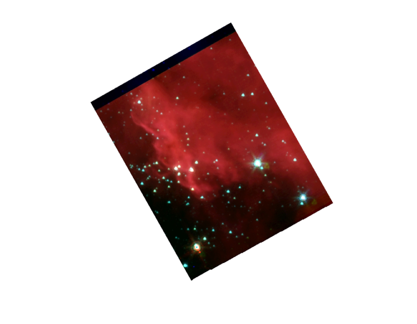
Figure 1: BRC 27, in the region of four-band IRAC coverage: IRAC-1 (3.6 $\mu$m; blue), IRAC-2 (4.5 $\mu$m; green), and IRAC-4 (8 $\mu$m; red). The pointing is a single dithered IRAC field of view, so about 5$\arcmin$ on a side. North is up. Both nebulosity and point sources can be seen.

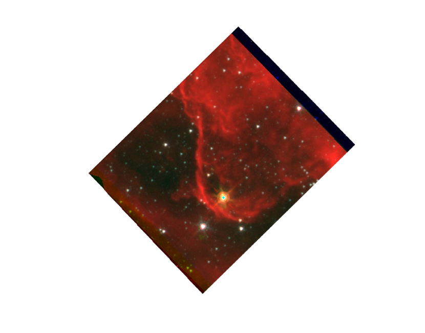
Figure 2: BRC 34, in the region of four-band IRAC coverage: IRAC-1 (3.6 $\mu$m; blue), IRAC-2 (4.5 $\mu$m; green), and IRAC-4 (8 $\mu$m; red). The pointing is a single dithered IRAC field of view, so about 5$\arcmin$ on a side. North is up. Both nebulosity and point sources can be seen.

We used the IRAC data for BRC 27 from Spitzer program 30050, AORKEY 17512192; for BRC 34, we used data from Spitzer program 202, AORKEY 6031616. The BRC 27 data were obtained on 2006-11-22, and were centered on $\alpha$=07:03:59, $\delta$=$-$11:23:09 (J2000); the BRC 34 data were obtained on 2004-07-04 and were centered on $\alpha$=21:33:32, $\delta$=+58:16:12.8 (J2000). Both AORs were 12 sec high-dynamic-range (HDR) frames, so there are two exposures at each pointing, 0.6 and 12 s, with 5 small-scale dithers per position, for a total integration time of 60 s (on average).

We started with the corrected basic calibrated data (CBCDs) processed using SSC pipeline version 18.18. We reprocessed the IRAC data, using MOPEX (Makovoz & Marleau 2005) to calculate frame-to-frame background matching (overlap) corrections and create mosaics with reduced instrumental artifacts compared to the pipeline mosaics. A 3-color mosaic for BRC 27 is shown in Fig. 1, and for BRC 34 in Fig. 2. The pixel size for our mosaics was 0.6$\arcsec$, identical to the SSC pipeline mosaics. This is half of the native pixel scale. We created separate mosaics for the long and the short exposures at each channel for photometric analysis.

In both BRCs, we focused our analysis on the region covered by all four IRAC bands, i.e., a region $\sim 5\arcmin\times 5\arcmin$ centered on the coordinates above. As a result of the way the instrument+telescope is designed, serendipitous data are obtained at two bands in each of two non-overlapping $\sim 5\arcmin\times 5\arcmin$ fields whose centers are offset $\sim 6.5\arcmin$ from the target field, in opposite directions; see the IRAC Instrument Handbook for more details. These regions with serendipitous data will be discussed in a forthcoming paper.

To obtain photometry of sources in each BRC region, we used the APEX-1frame module from MOPEX to perform source detection on the resultant long and short mosaics for each observation separately. We took those source lists and used the aper.pro routine in IDL to perform aperture photometry on each of these source detections in the corresponding mosaics with an aperture of 3 native pixels (6 resampled pixels), and an annulus of 3-7 native pixels (6-14 resampled pixels). The corresponding (multiplicative) aperture corrections are, for the four IRAC channels, 1.124, 1.127, 1.143, & 1.234, respectively, as listed in the IRAC Instrument Handbook. As a check on this automatic photometry, the educators and students associated with this project used the Aperture Photometry Tool (APT; Laher et al. 2012a,b) to confirm by hand the measurements for all the targets of interest (i.e., they inspected and clicked individually on each of the objects in each of the bands). To convert the flux densities to magnitudes, we used the zero points as provided in the IRAC Instrument Handbook: 280.9, 179.7, 115.0, and 64.13 Jy, respectively, for the four channels. (No array-dependent color corrections nor regular color corrections were applied.) We took the errors as produced by IDL to be the best possible internal error estimates; to compare to flux densities from other sources, we took a flat error estimate of 5% added in quadrature.

At this point in the process, for each BRC, we have one source list for each exposure time, for each channel, so a total of 8 source lists per BRC target. To obtain one source list per channel per BRC observation, we then merged the short and the long exposure source lists for each channel separately. We performed this merging via a strict by-position search, looking for the closest match within 1$\arcsec$. This maximum radius for matching was determined via experience with this analysis step in other star-forming regions (e.g., Rebull et al. 2010). If a match between the source lists was found, if the source is brighter than a threshold, the photometry was used from the short frame, and if it was fainter, then the photometry was taken from the long frame. The brightness thresholds beyond which photometry was obtained from the IRAC short exposures follows from the IRAC study of the Taurus star-forming region (Rebull et al. 2010, Padgett et al., in prep). They are 9.5, 9.0, 8.0, & 7.0 mag for the four IRAC channels respectively. The limiting magnitudes of these final source lists are the same for both observations, and are [3.6]$\sim$14 mag, [4.5]$\sim$14 mag, [5.8]$\sim$12 mag, and [8]$\sim$10.5 mag.

3.2 MIPS Data

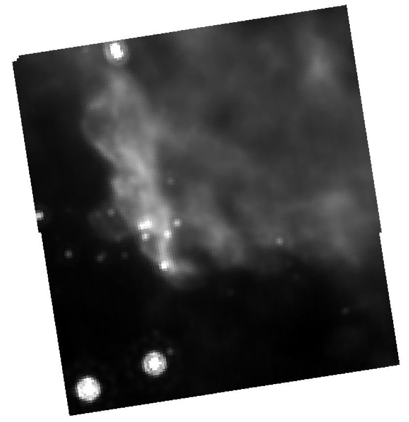
Figure 3: BRC 27 in 24 $\mu$m. The 70 $\mu$m image (not shown) is more or less featureless nebulosity. North is up; the image is $\sim$7.5$\arcmin$ on a side. Both nebulosity and point sources can be seen here.

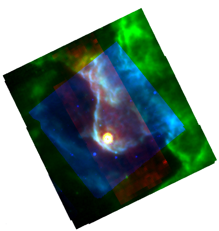
Figure 4: BRC 34 in 8 $\mu$m (blue), 24 $\mu$m (green) and 70 $\mu$m (red); note that all three bands have a slightly different footprint on the sky. North is up. The bright point source near the center has counterparts at all bands. The 24 $\mu$m band mosaic (the largest here) is $\sim$7.5$\arcmin$ on a side. Both nebulosity and point sources can be seen here.

We again used the MIPS data for BRC 27 from Spitzer program 30050, AORKEY 17512448, obtained on 2006-11-04; for BRC 34, we used data from Spitzer program 202, AORKEY 6031872, obtained on 2004-10-19.

In BRC 27, the AOR was designed to obtain two cycles of large-field photometry mode observations at 24 $\mu$m (with a 10$\arcsec$ sky offset), with 3 s per exposure. In BRC 34, the AOR was designed to obtain three cycles of small-field photometry, 3 s per exposure, at 24 $\mu$m. For both BRCs, the AORs also obtained one cycle of small-field default-scale mode observations at 70 $\mu$m. These observations are centered on the same location as the 4-band IRAC data. The final 24 $\mu$m coverage is $\sim$7.5$\arcmin$ on a side, so slightly larger than the four-band IRAC coverage (i.e., the region covered by all four IRAC bands), with 3 s per pointing and a maximum integration of 42 s only in the center $\sim 3\arcmin\times 3\arcmin$ portion for BRC 27, and 126 seconds in the center portion for BRC 34. The final 70 $\mu$m coverage is $\sim 3\arcmin\times 7.5\arcmin$, with a total of 30 s integration (3 s per pointing, one cycle). We note for completeness that serendipitous data with a field center about 12$\arcmin$ offset from of our target were obtained at 24 $\mu$m during the 70 $\mu$m photometry integration (see the MIPS Instrument Handbook for more information); since these fall outside of the 4-band IRAC coverage, they are beyond the scope of this paper and will be included in a forthcoming paper.

The data for 24 $\mu$m required additional processing beyond what the MIPS pipelines provided. We started with S18.12 enhanced BCDs (eBCDs) from the pipeline and created mosaics using MOPEX, as for IRAC. Our mosaics were constructed to have the same pixel size as the pipeline mosaics, 2.45$\arcsec$. The MIPS data for BRC 27 appear in Figure 3. The 70 $\mu$m data for BRC 27 revealed no point sources, and appears to be essentially featureless nebulosity, so we did not process it beyond the pipeline. The 70 $\mu$m data for BRC 34, on the other hand, had point sources and texture in the nebulosity. The pipeline produces both filtered and unfiltered mosaics; the filtering preserves the flux densities of the point sources and improves their signal-to-noise, especially for faint sources, but destroys the flux density information for the extended emission. The unfiltered mosaic is shown in Figure 4, but we performed photometry on the filtered mosaic. The pipeline mosaics have resampled 4$\arcsec$ pixels (as opposed to 5.3$\arcsec$ native pixels).

To obtain photometry at 24 $\mu$m (and 70 $\mu$m for BRC 34), we ran APEX-1frame on each of the mosaics and performed point-response-function (PRF) fitting photometry using the SSC-provided PRF. We used the signal-to-noise ratio (SNR) value returned by APEX-1frame as the best estimate of the internal (statistical) errors, adding a 4% flux density error in quadrature as a best estimate of the absolute uncertainty. For some sources of interest below, an upper limit at 24 $\mu$m was obtained at the given position by laying down an aperture as if a source were there, and taking 3 times that value for the 3$\sigma$ limit. For the single 70 $\mu$m detection, we assumed a conservative, flat 20% flux density error. (A second, fainter 70 $\mu$m source is visible in Fig. 4; this source is literally on the edge of the mosaic, and as such we cannot obtain reliable photometry for it.) To convert the flux densities to magnitudes, we used the zero points as found in the MIPS Instrument Handbook, 7.14 Jy and 0.775 Jy for 24 and 70 $\mu$m, respectively.

3.3 Optical Data

Based on experience with other star forming regions (e.g., Rebull et al. 2010, 2011c, Guieu et al. 2010), we know that optical data (either just photometric points or higher spatial resolution images, or both) can be tremendously helpful in discriminating between true YSOs and background galaxies. We obtained observations of our target region from the 2-m Las Cumbres Observatory Global Telescope (LCOGT) Network member telescope, Faulkes Telescope North (FTN), on Haleakala. The Faulkes telescope has a $\sim 10\arcmin$ field of view, easily encompassing our region of interest in both BRCs. The spatial resolution of the telescope is $\sim$1.1$\arcsec$, most often seeing-limited; this is well-matched to our $\sim$1.5$\arcsec$ resolution IRAC data. The pixel scale is 0.3$\arcsec$ pixel^-1.

The filters that we used were Sloan $r$ and $i$ bands. While there is no Sloan Digital Sky Survey (SDSS; Abazajian et al. 2009) coverage of our target, there are some reasonably nearby (on the sky) SDSS observations that we used to “bootstrap” our calibration. We obtained calibration images close in time (and in airmasses) to our science images; for BRC 27, the calibration image was at $\alpha\sim 7.6^{h},\delta\sim-11\arcdeg$, and for BRC 34, the calibration image was at $\alpha\sim 20.7^{h},\delta\sim+58\arcdeg$. The BRC 34 data were obtained on 2011-10-21, and the BRC 27 data were obtained on 2012-01-02. The images are initially processed through the LCOGT pipeline, which performs the bias and flatfield corrections. For BRC 34, it attached a world coordinate system (WCS) to the header, but it failed to do so in the case of BRC 27. We used astrometry.net to attach a WCS in that case. The science exposures were all 120 sec. The calibration frames for BRC 27 were also all 120 sec; the initial calibration frames for BRC 34 were 360 sec in $r$ and 240 sec in $i$, and then the final calibration frames were 120 sec. We took this into account in our data reduction. The observations were all obtained through about 1.3 airmasses. We used APT to obtain source detections for the calibration fields, and matched the sources in the calibration fields to the existing SDSS data sets using a conservative source matching of 1$\arcsec$ radius. There were between 177 and 303 sources of moderate brightness, depending on field and filter band, that were used to establish calibration for the science target fields. We used an 8 pixel aperture radius and a sky annulus from 9 to 15 pixels.

As for the calibration fields, we used APT using the same settings to detect and measure photometry for objects in the science fields, and applied our calibration solutions to the science fields. We again used an 8 pixel aperture radius and a sky annulus from 9 to 15 pixels. To match the much smaller subset of science target sources of interest between the two optical bands, in each pointing, we used a 2$\arcsec$ matching radius; empirically, this provided the best results. The completeness limits of these observations were $r\sim 20$, and $i\sim 19$, using Sloan (AB) magnitudes (Oke & Gunn 1983). We took the errors as produced by APT to be the best possible internal error estimates; to compare to flux densities from other sources, we took a flat, conservative absolute error estimate of 6% added in quadrature. If the objects are legitimately young, their intrinsic variability (due to cool star spots or accretion hot spots) at these wavelengths is likely to be larger than these error estimates. To convert these magnitudes to fluxes (for inclusion in the SEDs in Section 5.3), we used the standard 3631 Jy as a zero point (see, e.g., Finkbeiner et al. 2004). If an object of interest was not automatically detected in the images, we examined the images at the location of the object, and obtained by hand either an upper limit or a measurement of the photometry of the detection. Limits as reported in Table 2 are 3$\sigma$ limits.

3.4 Bandmerging and the Final Catalog

In summary, to bandmerge our data, we first merged the photometry from all four IRAC channels together with near-IR 2MASS data within each BRC observation, followed by MIPS data, and then the optical data. We now discuss each of these steps in more detail. We then compare our catalog to the literature catalog which we established in §2.

To merge the photometry from all four IRAC channels together, we started with a source list from 2MASS. This 2MASS source list includes $JHK_{s}$ photometry and limits, with high-quality astrometry. We merged this 2MASS source list by position to the IRAC-1 source list, using a search radius of 1$\arcsec$, a value empirically determined via experience with other star-forming regions (e.g., Rebull et al. 2010). Objects appearing in the IRAC-1 list but not the $JHK_{s}$ list were retained as new potential sources. The master catalog was then merged, in succession, to IRAC-2, 3, and 4, again each using a matching radius of 1$\arcsec$. Because the source detection algorithm we used can erroneously detect instrumental artifacts as point sources, we explicitly dropped objects seen only in one IRAC band as likely artifacts.

The MIPS 24 $\mu$m source list was then combined into the merged 2MASS+IRAC catalog, using a positional source match radius of 2$\arcsec$, again determined via experience with other star-forming regions (e.g., Rebull et al. 2010). The MOPEX source detection algorithm can erroneously report structure in the nebulosity as a chain of point sources found in the image, and by inspection, this was the case for these data. To weed out these false ‘sources’, we dropped objects from the catalog that were detections only at 24 $\mu$m and no other bands. There is only one 70 $\mu$m source (in BRC 34), so that was added by hand into the master catalog, matched to the appropriate source.

Finally, to merge the $J$ through 70 $\mu$m catalog to the optical ($ri$) catalog, we looked for nearest neighbors within 2$\arcsec$. That matching radius was determined empirically to be the best via comparison of these images and catalogs.

To put these observations in context with other similar surveys (e.g., Rebull et al. 2011b), BRC 27 has $\sim$220 sources with IRAC-1, $\sim$120 sources with IRAC-4, and $\sim$24 sources with MIPS 24 $\mu$m (and $\sim$180 sources with 2MASS data). BRC 34 has $\sim$580 sources with IRAC-1, $\sim$120 sources with IRAC-4, and only 5 sources with MIPS 24 $\mu$m (and $\sim$200 sources with 2MASS data).

The strong falloff of source numbers with increasing wavelength is typical for these bandpasses for the following reasons. The SED for stars without dust can be approximated by a blackbody curve, $\lambda B_{\lambda}=\left(\frac{2hc^{2}/\lambda^{4}}{\exp(hc/\lambda kT)-1)}\right)$ where $h$ is Planck’s constant, $c$ is the speed of light, $\lambda$ is wavelength, $k$ is Boltzmann’s constant, and $T$ is the temperature of the blackbody (or $T_{\rm eff}$ for a stellar approximation); $\lambda B_{\lambda}$ (rather than $B_{\lambda}$) is in units of energy density (e.g., erg s^-1 cm^-2) for the SED. At the wavelengths in the mid-infrared (between roughly 3 and 70 microns as considered here), the SED falls off as $\lambda^{-3}$. For six theoretical, equally sensitive channels at 3.6, 4.5, 5.8, 8, 24, and 70 microns, the expected brightness from a dust-free star would fall through these bands, and one would expect many fewer sources, say, at 70 $\mu$m compared to 3.6 $\mu$m. In reality, IRAC-1 and 2 (3.6 and 4.5 $\mu$m) are comparably sensitive. However, for these observations as conducted, IRAC-3 (5.8 $\mu$m) is very roughly 4 times less sensitive than IRAC-1 and 2, and IRAC-4 (8 $\mu$m) is very roughly 3 times less sensitive. The two different MIPS 24 $\mu$m observations have different integration times, so a sensitivity calculation for these observations indicates that these observations are very roughly 2-4 times less sensitive than IRAC-1 and 2. The MIPS 70 $\mu$m observations integrate to 30 s; the resulting sensitivity of these observations is nearly 200 times less sensitive than IRAC-1 and 2. Most of the sources seen in any given Spitzer image are photospheres (stars without dust), and as such their expected flux density falls steadily through the 2-70 $\mu$m range. Moreover, the sensitivity worsens essentially steadily through this same wavelength region, very roughly as $\lambda^{2.5}$ in an SED plot. So, the expected net source counts fall rapidly with increasing wavelength due both to the intrinsic falloff of the stellar SEDs with wavelength and the decreasing sensitivity of the observations with wavelength.

The difference in source count rates in IRAC-1 between the two BRCs can be traced to the number density of Galactic foreground and background stars. The Galactic coordinates of BRC 27 are $(l,b)$ = (224$\arcdeg$, $-2\arcdeg$) and for BRC 34, they are (99$\arcdeg$,$+5\arcdeg$). Given these positions, there are more foreground and/or background objects for BRC 34. Most foreground/background objects do not have IR excesses, and, thus, do not have counterparts detected in the longer Spitzer bandpasses. Most of the objects seen in these images are not young stars, but instead contaminants (background or foreground objects).

4 Selection of YSO Candidates with Infrared Excess

With our new multi-wavelength view of the two BRC regions, we can begin to look for young stars. We focus on finding sources having an infrared excess characteristic of YSOs surrounded by a dusty envelope and/or disk. In this Section, first we provide an overview of the color selection we used primarily to identify young stars (Section 4.1). Then we discuss the IRAC color-color diagram (Section 4.2), the IRAC and MIPS color-magnitude diagram (Section 4.3), the IRAC color-magnitude diagram (Section 4.4), and remaining literature objects without apparent IR excesses (Section 4.5). We summarize the entire process in Section 4.6. Two tables are provided in this section: Table 2 provides multi-band measurements of the YSOs and YSO candidates discussed here, and Table 3 summarizes notes about specific objects called out in the text.

4.1 Overview of Color Selection

There is no single Spitzer color selection criterion (or set of criteria) that is 100% reliable in separating members from non-member contaminants. Many have been considered in the literature (e.g., Allen et al. 2004, Rebull et al. 2007, Harvey et al. 2007, Gutermuth et al. 2008, 2009, Rebull et al. 2010, 2011a). Some make use of just MIPS bands, some make use of just IRAC bands, most use a series of many color criteria, and where possible, they make use of (sometimes substantial) ancillary data. One of the earliest methods was presented in Allen et al. (2004), which marked out regions of IRAC color-color space as most likely to harbor objects of various classes, but likely also include contaminants. The best general choice for selecting YSO candidates from Spitzer+2MASS data is the approach developed by Gutermuth et al. (2008, 2009). This selection method starts from the set of objects detected at all four IRAC bands and uses 2MASS and MIPS data where possible. It implements a series of (many) color cuts to attempt to remove contaminants such as background galaxies (usually red and faint) and knots of nebulosity. The most common contaminants left by any of these color selections are active galactic nuclei (AGN) and asymptotic giant branch (AGB) stars, both of which can have similar colors to legitimate YSOs (see, e.g., Stern et al. 2005 for AGN and Blum et al. 2006 for AGBs). YSOs generally are bright and red, though, depending on distance, mass, and degree of reddening and/or embeddedness, they can also be faint and red (see, e.g., Rebull et al. 2010, 2011a and references therein).

The regions of interest for our study are small areas on the sky, and we do not have reliable high-resolution extinction maps for these regions. We have used the Gutermuth method as adapted by Guieu et al. (2009, 2010) for the case in which no extinction map is available. In these BRC cases, the lack of an extinction map and subsequent lack of reddening-corrected steps in the selection process may erroneously include, in particular, bright background AGB stars. To attempt to compensate, once we have identified potential YSO candidates, we inspect each of these candidates in all available images, check their position in color-color and color-magnitude diagrams, and construct and inspect their SEDs. On the basis of this inspection, we drop objects that are most likely bright foreground or distant background objects, have insignificant IR excesses once errors are incorporated, are evidently contaminated by an image artifact or bright nearby source, or are clearly not point sources. In the process of doing this, when we construct color-color and color-magnitude diagrams, we identify objects that are worth investigating as additional YSO candidates due to their location in the diagram but were not picked up by the color cuts. Such objects were either originally missing a detection in a band that would have enabled automatic identification as a YSO candidate by the method we have implemented, or have such subtle excesses that the method didn’t identify them a priori. As such, our sample is not a statistically unbiased sample, but our goal was to obtain a complete sample of YSOs rather than an unbiased sample.

Table 2 includes all of the measurements for all of the literature YSOs, literature YSO candidates, and new YSO candidates that survived this selection and weeding process. Table 3 collects notes on the objects (as in, if an object is called out elsewhere in the paper, it is noted in Table 3), including identifying those literature YSOs or literature YSO candidates that do not seem to have an IR excess. In some cases where our individual inspection and evaluation suggests the IR excess may be marginal, we have identified the IR excess as uncertain in Table 3. We next discuss the distribution of these objects in several color-color and color-magnitude diagrams, highlighting some objects as necessary. In each case, we discuss where YSOs and contaminants are most likely to fall.

4.2 IRAC Color-Color Diagram

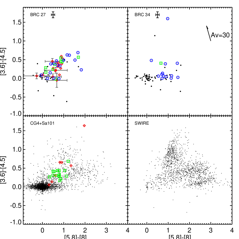
Figure 5: [3.6]$-$[4.5] vs. [5.8]$-$[8] color-color diagram for BRC 27 (upper left) and BRC 34 (upper right), with CG4+Sa101 (lower left) and SWIRE (lower right) for comparison. In each panel, small dots are objects in the catalog (i.e., objects seen in the image); green squares are literature high-confidence YSOs, red diamonds are literature candidate YSO, and blue circles are our new candidate YSOs presented here. Typical errors on the BRC data are $\sim$0.08 mags, and are indicated by the sample error bars in the top left of each of the BRC plots. Objects with exceptionally large error bars have error bars overplotted in grey. A sample $A_{V}$=30 vector is included in the BRC 34 panel for reference. The CG4+Sa101 and SWIRE data are provided for comparison to other fields, where there are foreground and background contaminants (stars and galaxies) in addition to YSOs; see text for more discussion. All of the YSOs (known, literature candidates, and new candidates) have colors in this diagram consistent with known YSOs, but many contaminants do too. Some of the YSOs and YSO candidates in BRC 27 have colors consistent with no IR excess. This is discussed further in the text.

Figure 5 shows the IRAC color-color diagram ([3.6]$-$[4.5] vs. [5.8]$-$[8]) for both BRC 27 and BRC 34, as well as two other fields for comparison. The lower left is the CG4+Sa101 data (see Section 2.1), and consists of background galaxies, foreground and background stars without IR excesses, and young stars (both high-confidence and candidate YSOs) with IR excesses. The lower right, for comparison, contains data from the 6.1 deg² Spitzer Wide-area Infrared Extragalactic Survey (SWIRE; Lonsdale et al. 2003) ELAIS (European Large Area ISO Survey) N1 extragalactic field (the Cores-to-Disks [c2d; Evans et al. 2003, 2009a] reduction is used here, as in Rebull et al. 2011a). This sample by its nature is expected to contain primarily galaxies, though likely includes some foreground stars not expected to have IR excesses. The SWIRE survey was relatively shallow compared to many extragalactic surveys, and as such provides a good comparison to these relatively shallow maps of galactic star forming regions.

By comparison of these panels in Figure 5, we can demonstrate where common objects are found. Ordinary stellar photospheres (likely foreground or background stars) are found near 0 in both IRAC colors; objects like this can be found most prominently in the CG4+Sa101 field, where there are many foreground or background stars. Galaxies are found throughout this diagram, but are often red in one or both colors, as can be seen in the SWIRE panel. YSOs with substantial IR excesses will be red in both [3.6]$-$[4.5] and [5.8]$-$[8]; YSOs with inner disk holes will have small [3.6]$-$[4.5] and red [5.8]$-$[8]. Objects with colors similar to YSOs can be seen in both BRC 27 and BRC 34.

Of the known YSOs, literature candidate YSOs, and new candidate YSOs considered here in the BRCs, most are red in both [3.6]$-$[4.5] and [5.8]$-$[8]. This is consistent with where we expect them to appear, based on YSOs studied elsewhere (e.g., in CG4+Sa101 in the lower left panel of the figure; Rebull et al. 2011b). However, many more known YSOs and literature YSO candidates are found in BRC 27 than in BRC 34. These previously identified YSOs and candidates were obtained via a variety of means not necessarily involving the IR, including X-rays (see §2). It is known that YSOs can be young without having circumstellar disks or envelopes (see §2.1 or, e.g., Rebull et al. 2010). Thus, YSOs may be legitimately young even though they do not have IR excesses. They may also have IR excesses at wavelengths longer than the longest wavelength used in this specific Figure, 8 $\mu$m. The YSO and YSO candidate objects with near 0 color in Fig. 5 are exactly these kinds of objects – possibly legitimately young, though not having an IR excess, or not having a detectable IR excess using these data and data reduction. We now discuss these objects because they are different than the rest of the ensemble of YSOs and YSO candidates in this diagram; notes on these objects appear in Table 3.

In BRC 27, five objects have [3.6]$-$[4.5]$<$0.1, and three of those also have the lowest [5.8]$-$[8] values, $<$ 0.03. Object 070352.2-112100 (=Chauhan 109=row 1 in the Tables) has a very small [3.6]$-$[4.5] but a larger [5.8]$-$[8]=0.5, so it appears to have a small excess at the longer bands, consistent with an inner disk hole. It is a literature YSO candidate, having been identified from an apparent NIR excess, which would be inconsistent with an inner disk hole, though we too identify it as having a small NIR excess (see §5.2 below). Follow-up spectroscopy might clarify this issue. Object 070352.7-112313 (=Ogura 2, Chauhan 81=row 2 in the Tables) has a very small [3.6]$-$[4.5] and a large, negative [5.8]$-$[8], suggesting that it does not have a disk; this object is quite faint at 8 $\mu$m, and as such, has a large error. The error is large enough that it could move it to [5.8]$-$[8]$\sim$0, consistent with other disk-free YSOs. It is also a literature YSO candidate, but it does not appear to have a measurable IR excess. Object 070353.8-112341 (=row 6 in the Tables) is a new YSO candidate. It has [3.6]$-$[4.5]=0.09 and [5.8]$-$[8]=$-$0.05, so it does not have much of an IRAC excess; it does, however, have a small excess at 24 $\mu$m (see Section 4.3). The fourth object, 070403.9-112609 (=Shevchenko 102=row 25 in the Tables), again has small [3.6]$-$[4.5] and [5.8]$-$[8], but with [3.6]$-$[4.5]$>$[5.8]$-$[8]. This one does not appear to have a measurable IR excess; it is a literature YSO candidate, so additional spectra would be particularly useful to determine if it is a foreground star or truly a member of BRC 27. Finally, object 070406.0-112128 (=row 33 in the Tables) is a new candidate YSO. It has [3.6]$-$[4.5]=0 and [5.8]$-$[8]=0.23, so it appears to have a small excess at the longer bands, consistent with an inner disk hole. It will be discussed again in Section 4.3 below, where it appears to have a quite significant [3.6]$-$[24] excess.

In BRC 34, one new YSO candidate object (213334.8+580409=row 51 in the Tables) has [5.8]$-$[8]$\sim$0.2 and [3.6]$-$[4.5]$\sim$0.5; it is somewhat unusual to have [3.6]$-$[4.5]$>$[5.8]$-$[8]; for inner disk holes, one generally expects [3.6]$-$[4.5]$<$[5.8]$-$[8]. This object also has the most extreme values of $J-H$ and $H-K_{s}$ (see §5.2 below). It is probably subject to considerable reddening, which accounts for the observation that [3.6]$-$[4.5]$>$[5.8]$-$[8] (see the reddening vector in Figure 5).

All the remaining YSOs and YSO candidates in these two BRCs have significant IRAC excesses. The largest [3.6]$-$[4.5] is found in BRC 34, 213332.2+580329 (=row 49 in the Tables); it also has a large 24 $\mu$m excess (see Section 4.3 below). It most likely is subject to significant reddening, which accounts for the fact that [3.6]$-$[4.5]$>$[5.8]$-$[8] (see the reddening vector in Figure 5). It is also the only source in either BRC detected at 70 $\mu$m.

4.3 IRAC & MIPS Color-Magnitude Diagram

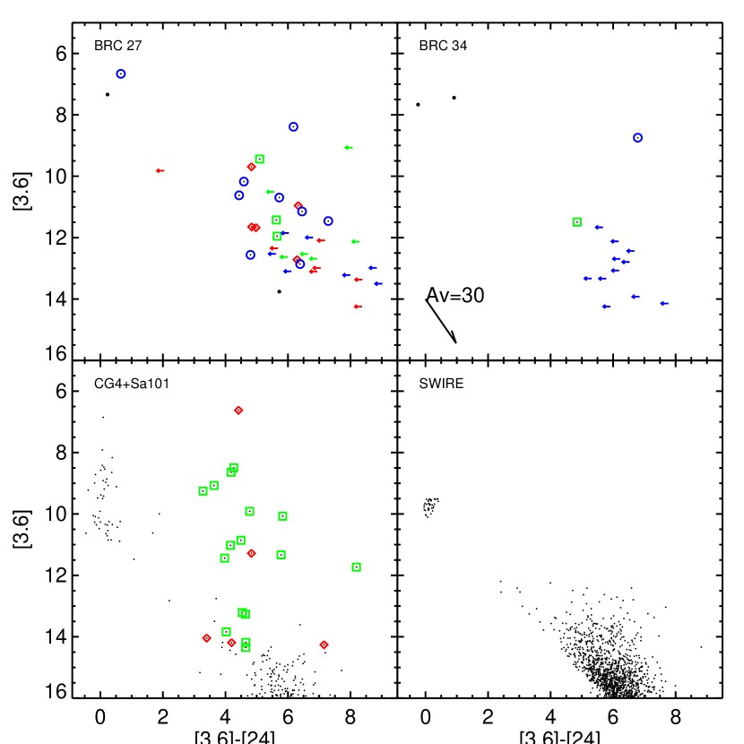
Figure 6: [3.6] vs. [3.6]$-$[24] color-magnitude diagram for BRC 27 (upper left) and BRC 34 (upper right), with CG4+Sa101 (lower left) and SWIRE (lower right) for comparison. In each panel, small dots are objects in the catalog (i.e., objects seen in the image); green squares are literature high-confidence YSOs (green arrows are limits for objects undetected in the 24 $\mu$m map), red diamonds are literature candidate YSO (red arrows are limits), and blue circles are our new candidate YSOs presented here (blue arrows are limits). Error bars are typically smaller than the symbol – 0.06 mags in [3.6] and 0.07 mags in [3.6]$-$[24]. No objects here have exceptionally large error bars. A sample $A_{V}$=30 vector is included in the BRC 34 panel for reference. There are very few sources seen at 24 $\mu$m in either of these BRC regions; the lower two panels give a better sense of the distribution of objects seen in general. All of the BRC 27 and BTRC 34 YSOs (known, literature candidates, and new candidates) have colors in this diagram consistent with known YSOs; see text for more discussion.

Young stars having inner disk holes and thus excesses at only the longest bands can be revealed in particular via comparison of the 24 $\mu$m or 8 $\mu$m measurement to a shorter band, such as 3.6 $\mu$m. Figure 6 shows [3.6] vs. [3.6]$-$[24] for both BRC 27 and BRC 34, as well as the CG4+Sa101 and SWIRE samples for comparison.

Since there are very few 24 $\mu$m sources detected that are not YSOs or YSO candidates in either BRC, it is easier to understand the expected distribution of sources by inspection of the CG4+Sa101 and SWIRE samples. Foreground or background stars have $[3.6]-[24]\sim$0, and galaxies likely make up the source concentration near [3.6]$-$[24]$\sim$6, [3.6]$\sim$16. Objects that are red and bright can be YSOs; since we are comparing [3.6] and [24] here, even disks with large inner disk holes will appear here as red. However, AGB stars can also occupy this part of the parameter space. As in Fig. 5, most of the YSOs and candidate YSOs (from the literature or new) that are detected are in fact in the location in this diagram expected for YSOs. Many objects are not detected at 24 $\mu$m, and those are indicated as limits for comparison. Many more objects are detected at 24 $\mu$m in CG4+Sa101 because the CG4+Sa101 [24] observation had a longer exposure time, and the sources that are members of CG4+Sa101 are brighter because CG4+Sa101 is considerably closer to us (3-500 pc vs. 800-1000 pc for the BRCs).

In the BRC 27 plot, one object (070406.0-112128 =row 33 in the Tables) appeared as having [3.6]$-$[24]$\sim$4.6 (and [3.6]$\sim$10.2), comfortably within the distribution of YSOs and candidates (it has a reasonably large [3.6]$-$[24]), but not having been picked a priori as a YSO using the Gutermuth method and the IRAC colors. This object was mentioned in Section 4.2 as having a very small IRAC excess at the longer wavelength bands. The object is in a region of relatively bright nebulosity at 8 and 24 $\mu$m; though it is clearly detected as a point source at 8 $\mu$m, its detection is less certain at 24 $\mu$m. Had this object only had an excess at 24 $\mu$m, we might attribute the apparent excess to nebular contamination. However, Fig. 5 and the SED (see §5.3.1 below) suggests that there might be a small excess at the two longest IRAC bands. In order to formally calculate the significance of any excess, we need a spectral type and model fitting to the SED, but we can extend a line with a Rayleigh-Jeans (RJ) slope (to approximate a blackbody) from the 2.2 $\mu$m or 3.6 $\mu$m point to get an approximate guess as to what the expected photospheric flux density might be, and then compare that to the measured flux density (including its error estimate). Performing this calculation suggests that the measured 8 $\mu$m detection of this object has a marginal significance of $\sim 4\sigma$. This measurement, while not significant on its own, is independent of the excess at 24 $\mu$m; the fact that it might be a excess suggests that nebula might not be the only contributor to any excess, and that there might be circumstellar dust around this object. This object could have a large inner disk hole, resulting in excess only at the longest wavelengths sampled here. We have included this object in our list as having a possible IR excess (see Table 3), but follow-up spectroscopy would be particularly important in this object’s case, because of the potential for contamination by the nebulosity (or an unresolved background object).

Also in the BRC 27 plot, the brightest YSO candidate object ([3.6]$\sim$6.5) is 070353.8-112341 (=row 6 in the Tables). This object was mentioned in Section 4.2 as having small IRAC colors. It is included in the set of new YSO candidates because it has an apparently marginally significant 24 $\mu$m excess, with [3.6]$-$[24]=0.65, which is not large in comparison to many of the other [3.6]$-$[24] values seen in Figure 6, but given the uncertainties on the photometry, and the approach above extending an RJ slope from 2.2 $\mu$m, the 24 $\mu$m excess is $\sim$11$\sigma$. It does not have a significant 8 $\mu$m excess. It is bright at IRAC bands, and clearly detected in the 24 $\mu$m image (see Figure 17 below), and not obviously contaminated by nebulosity. There is a reasonable chance that this is a foreground star and that the photometry is compromised, or it is a very interesting object with a very large inner disk hole (potentially containing protoplanets); follow up spectroscopy is necessary. We have tagged it as an uncertain IR excess in Table 3.

The bluest limit in BRC 27 (at [3.6]$\sim$10 and [3.6]$-$[24]$\sim$2) is 070403.9-112609 (=Shevchenko 102=row 25). This object was mentioned in Section 4.2 above as not having a significant IRAC excess. It is not detected at 24 $\mu$m, which is consistent with either a small excess at 24 $\mu$m or no excess at all. We do not detect a MIR excess in this object.

The brightest YSO candidate in BRC 34 also has the largest detectable [3.6]$-$[24] in BRC 34, and it is 213332.2+580329 (=row 49 in the Tables). This object is also the only object in either BRC detected at 70 $\mu$m.

4.4 IRAC Color-Magnitude Diagram

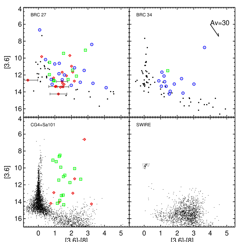
Figure 7: [3.6] vs. [3.6]$-$[8] color-magnitude diagram for BRC 27 (upper left) and BRC 34 (upper right), with CG4+Sa101 (lower left) and SWIRE (lower right) for comparison. In each panel, small dots are objects in the catalog (i.e., objects seen in the image); green squares are literature high-confidence YSOs, red diamonds are literature candidate YSO, and blue circles are our new candidate YSOs presented here. Error bars are typically smaller than the symbol – 0.06 mags in [3.6] and 0.07 mags in [3.6]$-$[8]. Objects with exceptionally large error bars have error bars overplotted in grey. A sample $A_{V}$=30 vector is included in the BRC 34 panel for reference. SWIRE data saturate at about [3.6]$\sim$9.5 because their IRAC data were not obtained in HDR mode (see §3.1). Most of the BRC 27 and BRC 34 YSOs (known, literature candidates, and new candidates) have colors in this diagram consistent with known YSOs; one of the previously-known YSOs in BRC 27 has an anomalously blue color but also large errors at [8]. See text for more discussion.

We also examined the [3.6] vs. [3.6]$-$[8] color-magnitude diagram; see Figure 7. Data from CG4+Sa101 and SWIRE are again included for context. As for Figure 6, foreground and background photospheres have [3.6]$-$[8]$\sim$0, and galaxies populate the clump at [3.6]$-$[8]$\sim$2 and [3.6]$\sim$16. Young stars are bright and red; since we are comparing [3.6] and [8] here, even disks with relatively large inner disk holes will appear here as red. However, AGB stars can also occupy this part of the parameter space. We investigated all of the objects that have YSO-like colors but were not identified in the color-selection method above. Several of these objects appear to have small excesses at 8 $\mu$m, which we now discuss.

From BRC 27, there are three objects worth considering that we identify from this Figure (as opposed to being selected via the Gutermuth-style color cuts above in Section 4.1). Object 070354.9-112514 (=Ogura 5, Chauhan 94=row 8 in the Tables) has no 24 $\mu$m data (it is off the edge of the MIPS-24 map). It appears in the grouping of sources near [3.6]$-$[8]$\sim$1 and [3.6]$\sim$13. It has only a $\sim$7$\sigma$ excess at 8 $\mu$m; it has a very weak possible 5.8 $\mu$m excess as well (see SED in Section 5.3.1). It is a literature YSO candidate. We have identified this object as having a very uncertain IR excess.

Object 070406.5-112227 (=row 36 in the Tables) has a nominal 8 $\mu$m excess at the $\sim$6$\sigma$ level, and no 24 $\mu$m detection. Like the prior object, it too has a very weak possible 5.8 $\mu$m excess (see SED in Section 5.3.1), and is grouping of sources near [3.6]$-$[8]$\sim$0.8 and [3.6]$\sim$13. We have also identified this object as having a very uncertain IR excess.

Object 070407.9-112311 (=Ogura 21=row 39 in the Tables) also appears somewhat red in this diagram, near [3.6]$-$[8]$\sim$0.9 and [3.6]$\sim$12. It has an 8 $\mu$m excess at the 11$\sigma$ level. The [5.8] point also does not appear to be photospheric (see Section 5.3.1); it is not detected at [24], and it may be subject to high $A_{V}$. We have identified this object as having an IR excess in Table 3.

A fourth object from BRC 27, object 070408.1-112313 (=row 41 in the Tables) is identified via the Gutermuth-style color cuts. It appears as somewhat red in this diagram, near [3.6]$-$[8]$\sim$0.8 and [3.6]$\sim$12.5. Like the other similar objects above, it has an 8 $\mu$m excess at the $\sim$7$\sigma$ level, and no 24 $\mu$m detection. However, it seems to have an excess beginning at [4.5], so it is identified as having a more confident IR excess in Table 3.

In BRC 34, six objects appear as red in Figure 7, none of which were selected via the Gutermuth-style color cuts above in Section 4.1. All of them have upper limits at 24 $\mu$m, all of them have 8 $\mu$m excesses $>$10$\sigma$, and all of them have possible low-significance 5.8 $\mu$m excesses. Most of them are near [3.6]$-$[8]$\sim$1-2 and [3.6]$\sim$12-14, as for similar objects from BRC 27 above. We have identified all of them as having IR excesses, though a case could be made for them being uncertain because of the contamination possible at [8]. They are: 213314.5+580351 (=row 43 in the Tables), 213315.6+580407 (=row 44), 213319.4+580406 (=row 45), 213323.8+580632 (=row 46; this is the reddest of this set at [3.6]$-$[8]$\sim$2 and [3.6]$\sim$14), 213332.2+580558 (=row 50), and 213334.8+580409 (=row 51); this last may also be subject to high $A_{V}$, as noted in Section 4.2, and it is also the brightest of this set, at [3.6]$-$[8]$\sim$1 and [3.6]$\sim$12.

4.5 Remaining Literature Objects Without Excesses

Object 070353.5-112350 (=Shevchenko 90=row 4 in the Tables) is a likely YSO from the literature, with an A0 spectral type. It is not detected at [24], the [8] point is only about 6$\sigma$ above the photosphere, and all the rest of the 2-5.8 $\mu$m points appear to be detecting the photosphere. It does not appear to have a significant IR excess.

We inspected object 070404.5-112555 (=Ogura 13=row 28 in the Tables) because it is identified in the literature as a candidate YSO. However, this object is not detected at [24], and it is only detected with very large errors at [5.8] and [8]. Taking into account the errors, the 8 $\mu$m excess is only significant at the 2.5$\sigma$ level. We do not identify this in Table 3 as having an excess.

For completeness, we mention here that 070403.9-112609 (=Shevchenko 102=row 25 in the Tables) and 070352.7-112313 (=Ogura 2, Chauhan 81=row 2 in the Tables) were discussed in Section 4.2 (and 4.3 for 070403.9-112609) as not having a measurable IR excess.

4.6 Summary of IR Excess Selection

In summary, we have 42 YSOs or YSO candidates (new or from the literature) in BRC 27, and 14 YSOs or new YSO candidates in BRC 34.

Of the 26 literature YSOs or literature YSO candidates in BRC 27, we find some indication of IR excess around 22 of them (one of those has an uncertain IR excess). Of the 9 high-confidence literature YSOs, 8 have high-confidence IR excesses, and one has no apparent IR excess. Of the 17 literature YSO candidates, 14 have IR excesses, one has an uncertain IR excess, and 3 have no detectable IR excess. There are 16 new YSO candidates presented here, 13 of which have IR excesses (and 3 of which have uncertain IR excesses).

BRC 34 is again simpler; the one literature YSO also has an IR excess. There are 13 new objects with IR excesses presented here.

We move ahead from here with this set of YSOs and YSO candidates, and now investigate their multi-band properties.

Table 2: Multiband measurements of known YSOs, literature YSO candidates, and new Spitzer-identified YSO candidates in BRC 27 and BRC 34

row	name	Alt. name	$r$	$i$	$J$	$H$	$K_{s}$	[3.6]	[4.5]	[5.8]	[8.0]	[24]	[70]
BRC 27
1	070352.2-112100	Chauhan109	20.92$\pm$ 0.22	19.50$\pm$ 0.09	15.71$\pm$ 0.06	14.59$\pm$ 0.07	13.78$\pm$ 0.05	13.37$\pm$ 0.05	13.32$\pm$ 0.05	12.83$\pm$ 0.06	12.34$\pm$ 0.39	$>$ 4.99	$\cdots$
2	070352.7-112313	Ogura2,Chauhan81	16.88$\pm$ 0.04	15.84$\pm$ 0.04	13.83$\pm$ 0.04	13.03$\pm$ 0.05	12.83$\pm$ 0.04	12.61$\pm$ 0.05	12.54$\pm$ 0.05	12.98$\pm$ 0.13	13.25$\pm$ 0.60	$\cdots$	$\cdots$
3	070353.2-112403	Ogura3	20.50$\pm$ 0.27	19.02$\pm$ 0.09	15.92$\pm$ 0.07	14.60$\pm$ 0.05	13.84$\pm$ 0.05	12.77$\pm$ 0.05	12.31$\pm$ 0.05	11.81$\pm$ 0.05	11.34$\pm$ 0.34	$\cdots$	$\cdots$
4	070353.5-112350	Shevchenko90	11.26$\pm$ 0.04	11.44$\pm$ 0.04	10.75$\pm$ 0.20	10.71$\pm$ 0.20	10.67$\pm$ 0.20	10.51$\pm$ 0.05	10.53$\pm$ 0.05	10.47$\pm$ 0.06	9.83$\pm$ 0.09	$>$ 4.95	$\cdots$
5	070353.7-112428	Ogura4,Chauhan82	19.23$\pm$ 0.07	17.54$\pm$ 0.04	15.04$\pm$ 0.04	14.22$\pm$ 0.05	13.94$\pm$ 0.06	13.44$\pm$ 0.05	13.17$\pm$ 0.05	12.61$\pm$ 0.06	12.10$\pm$ 0.06	$\cdots$	$\cdots$
6	070353.8-112341	$\cdots$	11.83$\pm$ 0.30	11.20$\pm$ 0.30	8.17$\pm$ 0.01	7.22$\pm$ 0.04	6.84$\pm$ 0.02	6.66$\pm$ 0.05	6.58$\pm$ 0.05	6.54$\pm$ 0.05	6.59$\pm$ 0.05	6.01$\pm$ 0.04	$\cdots$
7	070354.6-112011	Chauhan108	20.37$\pm$ 0.14	19.10$\pm$ 0.07	15.93$\pm$ 0.07	14.98$\pm$ 0.08	14.37$\pm$ 0.07	14.25$\pm$ 0.05	14.03$\pm$ 0.06	13.66$\pm$ 0.18	13.03$\pm$ 0.51	$>$ 5.88	$\cdots$
8	070354.9-112514	Ogura5,Chauhan94	18.00$\pm$ 0.05	16.74$\pm$ 0.04	14.62$\pm$ 0.03	13.83$\pm$ 0.04	13.59$\pm$ 0.05	13.34$\pm$ 0.05	13.24$\pm$ 0.05	13.07$\pm$ 0.07	12.27$\pm$ 0.09	$\cdots$	$\cdots$
9	070357.1-112432	Ogura7,Chauhan83	18.40$\pm$ 0.05	17.12$\pm$ 0.04	14.82$\pm$ 0.03	13.98$\pm$ 0.02	13.74$\pm$ 0.05	13.11$\pm$ 0.05	12.75$\pm$ 0.05	12.32$\pm$ 0.06	11.55$\pm$ 0.06	$>$ 6.17	$\cdots$
10	070358.4-112325	$\cdots$	13.39$\pm$ 0.04	13.19$\pm$ 0.04	12.32$\pm$ 0.02	11.97$\pm$ 0.03	11.92$\pm$ 0.03	11.85$\pm$ 0.05	11.86$\pm$ 0.05	11.38$\pm$ 0.07	10.61$\pm$ 0.05	$>$ 5.82	$\cdots$
11	070400.7-112323	$\cdots$	$>$ 20.60	$>$ 20.68	15.71$\pm$ 0.06	13.16$\pm$ 0.03	11.80$\pm$ 0.02	10.69$\pm$ 0.05	10.31$\pm$ 0.05	10.10$\pm$ 0.05	9.70$\pm$ 0.05	4.97$\pm$ 0.04	$\cdots$
12	070401.2-112531	$\cdots$	18.74$\pm$ 0.05	17.53$\pm$ 0.05	14.26$\pm$ 0.03	12.96$\pm$ 0.02	11.98$\pm$ 0.02	10.62$\pm$ 0.05	10.22$\pm$ 0.05	9.90$\pm$ 0.05	9.36$\pm$ 0.05	6.18$\pm$ 0.04	$\cdots$
13	070401.2-112242	$\cdots$	$>$ 22.55	$>$ 20.47	16.27$\pm$ 0.09	14.94$\pm$ 0.08	13.82$\pm$ 0.05	12.86$\pm$ 0.05	12.23$\pm$ 0.05	11.49$\pm$ 0.06	10.32$\pm$ 0.06	6.47$\pm$ 0.06	$\cdots$
14	070401.2-112233	Chauhan-anon	$>$ 23.01	$>$ 19.16	15.91$\pm$ 0.07	14.50$\pm$ 0.07	13.72$\pm$ 0.05	12.99$\pm$ 0.05	12.67$\pm$ 0.05	12.25$\pm$ 0.06	11.52$\pm$ 0.06	$>$ 5.94	$\cdots$
15	070401.3-112334	Gregorio74,Chauhan-anon	13.99$\pm$ 0.04	13.48$\pm$ 0.04	11.45$\pm$ 0.20	10.84$\pm$ 0.20	10.33$\pm$ 0.20	9.44$\pm$ 0.05	9.07$\pm$ 0.05	8.50$\pm$ 0.06	7.92$\pm$ 0.05	4.35$\pm$ 0.04	$\cdots$
16	070401.6-112406	$\cdots$	18.52$\pm$ 0.15	18.38$\pm$ 0.15	16.59$\pm$ 0.12	14.89$\pm$ 0.12	13.65$\pm$ 0.06	11.46$\pm$ 0.05	10.84$\pm$ 0.05	9.95$\pm$ 0.07	8.69$\pm$ 0.05	4.17$\pm$ 0.04	$\cdots$
17	070401.6-112132	$\cdots$	$>$ 20.25	19.47$\pm$ 0.09	15.36$\pm$ 0.04	13.85$\pm$ 0.03	12.98$\pm$ 0.03	12.00$\pm$ 0.05	11.64$\pm$ 0.05	11.13$\pm$ 0.06	10.42$\pm$ 0.07	$>$ 5.19	$\cdots$
18	070402.1-112512	$\cdots$	$>$ 20.23	19.79$\pm$ 0.14	15.95$\pm$ 0.08	14.72$\pm$ 0.11	14.05$\pm$ 0.07	12.56$\pm$ 0.05	12.09$\pm$ 0.05	11.78$\pm$ 0.06	11.12$\pm$ 0.05	7.76$\pm$ 0.09	$\cdots$
19	070402.2-112542	$\cdots$	12.06$\pm$ 0.04	12.09$\pm$ 0.04	11.31$\pm$ 0.03	10.75$\pm$ 0.03	9.94$\pm$ 0.05	8.39$\pm$ 0.05	7.70$\pm$ 0.05	6.83$\pm$ 0.05	5.16$\pm$ 0.05	2.21$\pm$ 0.04	$\cdots$
20	070402.3-112539	Shevchenko99,Gregorio75	11.09$\pm$ 0.04	11.23$\pm$ 0.04	10.40$\pm$ 0.04	10.32$\pm$ 0.07	10.26$\pm$ 0.02	9.07$\pm$ 0.05	8.50$\pm$ 0.05	7.91$\pm$ 0.05	6.22$\pm$ 0.05	$>$ 1.00	$\cdots$
21	070402.7-112325	$\cdots$	$>$ 22.44	$>$ 19.55	$\cdots$	13.94$\pm$ 0.10	12.58$\pm$ 0.04	11.15$\pm$ 0.05	10.66$\pm$ 0.05	9.95$\pm$ 0.06	8.96$\pm$ 0.08	4.70$\pm$ 0.07	$\cdots$
22	070402.9-112337	Ogura8+9,Chauhan84	17.51$\pm$ 0.04	16.26$\pm$ 0.04	13.56$\pm$ 0.04	12.43$\pm$ 0.05	11.86$\pm$ 0.03	10.96$\pm$ 0.05	10.54$\pm$ 0.05	9.71$\pm$ 0.05	8.95$\pm$ 0.05	4.63$\pm$ 0.04	$\cdots$
23	070403.0-112350	Ogura10,Chauhan85	19.04$\pm$ 0.06	17.82$\pm$ 0.05	15.68$\pm$ 0.06	14.34$\pm$ 0.04	13.55$\pm$ 0.04	12.13$\pm$ 0.05	11.69$\pm$ 0.05	10.76$\pm$ 0.08	9.83$\pm$ 0.05	$>$ 3.84	$\cdots$
24	070403.1-112327	Chauhan107	18.38$\pm$ 0.05	16.94$\pm$ 0.05	13.03$\pm$ 0.04	11.57$\pm$ 0.04	10.69$\pm$ 0.02	9.69$\pm$ 0.05	9.31$\pm$ 0.05	8.69$\pm$ 0.06	7.79$\pm$ 0.07	4.86$\pm$ 0.15	$\cdots$
25	070403.9-112609	Shevchenko102	10.62$\pm$ 0.04	10.74$\pm$ 0.04	9.76$\pm$ 0.02	9.72$\pm$ 0.03	9.63$\pm$ 0.02	9.82$\pm$ 0.05	9.73$\pm$ 0.05	9.65$\pm$ 0.05	9.62$\pm$ 0.05	$>$ 7.78	$\cdots$
26	070403.9-112326	$\cdots$	$>$ 20.37	$>$ 19.80	16.75$\pm$ 0.14	15.31$\pm$ 0.10	14.22$\pm$ 0.06	12.98$\pm$ 0.05	12.50$\pm$ 0.06	11.21$\pm$ 0.05	9.68$\pm$ 0.07	$>$ 4.14	$\cdots$
27	070404.2-112355	Ogura12,Chauhan86	18.61$\pm$ 0.05	17.52$\pm$ 0.04	15.01$\pm$ 0.04	14.02$\pm$ 0.04	13.54$\pm$ 0.05	12.53$\pm$ 0.05	12.08$\pm$ 0.05	11.60$\pm$ 0.05	10.73$\pm$ 0.05	$>$ 5.89	$\cdots$
28	070404.5-112555	Ogura13	18.11$\pm$ 0.05	16.89$\pm$ 0.04	14.77$\pm$ 0.03	13.88$\pm$ 0.02	13.73$\pm$ 0.04	13.40$\pm$ 0.09	13.45$\pm$ 0.17	12.58$\pm$ 0.34	11.91$\pm$ 0.34	$\cdots$	$\cdots$
29	070404.7-112339	Ogura14,Chauhan87	17.61$\pm$ 0.04	16.61$\pm$ 0.04	14.16$\pm$ 0.04	13.09$\pm$ 0.04	12.51$\pm$ 0.04	11.67$\pm$ 0.05	11.26$\pm$ 0.05	10.90$\pm$ 0.06	10.23$\pm$ 0.10	6.70$\pm$ 0.19	$\cdots$
30	070405.1-112313	Ogura15,Chauhan88	19.91$\pm$ 0.11	18.84$\pm$ 0.07	14.49$\pm$ 0.07	13.27$\pm$ 0.07	12.46$\pm$ 0.04	11.42$\pm$ 0.05	10.88$\pm$ 0.05	10.22$\pm$ 0.05	9.36$\pm$ 0.05	5.80$\pm$ 0.04	$\cdots$
31	070405.7-112123	$\cdots$	$>$ 18.08	$>$ 17.82	15.86$\pm$ 0.20	14.80$\pm$ 0.20	14.25$\pm$ 0.11	13.22$\pm$ 0.05	12.89$\pm$ 0.06	12.05$\pm$ 0.10	11.23$\pm$ 0.06	$>$ 5.23	$\cdots$
32	070405.9-112358	Ogura16,Chauhan89	17.90$\pm$ 0.04	16.88$\pm$ 0.04	14.42$\pm$ 0.03	13.47$\pm$ 0.03	12.93$\pm$ 0.03	11.65$\pm$ 0.05	11.12$\pm$ 0.05	10.51$\pm$ 0.05	9.57$\pm$ 0.05	6.81$\pm$ 0.04	$\cdots$
33	070406.0-112128	$\cdots$	11.86$\pm$ 0.04	11.68$\pm$ 0.06	10.64$\pm$ 0.03	10.41$\pm$ 0.02	10.26$\pm$ 0.02	10.18$\pm$ 0.05	10.18$\pm$ 0.05	9.98$\pm$ 0.06	9.74$\pm$ 0.07	5.59$\pm$ 0.04	$\cdots$
34	070406.0-112315	Ogura17,Chauhan90	19.14$\pm$ 0.07	17.92$\pm$ 0.05	15.11$\pm$ 0.06	13.97$\pm$ 0.04	13.25$\pm$ 0.03	12.72$\pm$ 0.05	12.13$\pm$ 0.05	11.43$\pm$ 0.06	10.54$\pm$ 0.06	6.43$\pm$ 0.04	$\cdots$
35	070406.4-112336	Ogura18,Chauhan91	20.01$\pm$ 0.13	17.79$\pm$ 0.05	14.70$\pm$ 0.05	13.81$\pm$ 0.05	13.36$\pm$ 0.07	12.69$\pm$ 0.05	12.40$\pm$ 0.05	11.89$\pm$ 0.07	11.73$\pm$ 0.06	$>$ 5.75	$\cdots$
36	070406.5-112227	$\cdots$	18.04$\pm$ 0.05	17.02$\pm$ 0.04	14.51$\pm$ 0.03	13.60$\pm$ 0.03	13.30$\pm$ 0.03	13.10$\pm$ 0.05	13.09$\pm$ 0.05	12.81$\pm$ 0.07	12.27$\pm$ 0.09	$>$ 6.99	$\cdots$
37	070406.5-112128	$\cdots$	19.11$\pm$ 0.15	18.55$\pm$ 0.15	15.87$\pm$ 0.14	15.27$\pm$ 0.14	14.75$\pm$ 0.11	13.50$\pm$ 0.05	13.27$\pm$ 0.05	11.22$\pm$ 0.08	9.40$\pm$ 0.08	$>$ 4.48	$\cdots$
38	070406.5-112316	Ogura19,Chauhan92	17.40$\pm$ 0.04	16.41$\pm$ 0.04	13.90$\pm$ 0.06	12.95$\pm$ 0.04	12.53$\pm$ 0.03	12.09$\pm$ 0.05	11.82$\pm$ 0.05	11.25$\pm$ 0.07	10.39$\pm$ 0.09	$>$ 4.91	$\cdots$
39	070407.9-112311	Ogura21	19.54$\pm$ 0.13	18.02$\pm$ 0.06	$>$ 14.35	14.23$\pm$ 0.09	13.68$\pm$ 0.07	12.35$\pm$ 0.05	12.14$\pm$ 0.05	12.02$\pm$ 0.06	11.42$\pm$ 0.06	$>$ 6.67	$\cdots$
40	070408.0-112354	Ogura22,Chauhan97	15.50$\pm$ 0.04	14.91$\pm$ 0.04	13.12$\pm$ 0.03	12.44$\pm$ 0.04	12.20$\pm$ 0.03	11.95$\pm$ 0.05	11.79$\pm$ 0.05	11.45$\pm$ 0.05	11.29$\pm$ 0.05	6.30$\pm$ 0.04	$\cdots$
41	070408.1-112313	$\cdots$	18.06$\pm$ 0.07	16.97$\pm$ 0.04	$>$ 14.29	13.77$\pm$ 0.09	13.50$\pm$ 0.09	12.53$\pm$ 0.06	12.38$\pm$ 0.06	12.12$\pm$ 0.06	11.75$\pm$ 0.07	$>$ 6.91	$\cdots$
42	070408.1-112309	Ogura23,Chauhan98	19.88$\pm$ 0.13	18.28$\pm$ 0.07	$\cdots$	14.59$\pm$ 0.06	14.19$\pm$ 0.07	12.63$\pm$ 0.06	12.39$\pm$ 0.05	12.22$\pm$ 0.06	11.72$\pm$ 0.06	$>$ 6.64	$\cdots$
BRC 34
43	213314.5+580351	$\cdots$	$>$ 17.55	$>$ 16.62	15.61$\pm$ 0.07	14.65$\pm$ 0.07	14.57$\pm$ 0.09	14.25$\pm$ 0.05	14.18$\pm$ 0.08	13.51$\pm$ 0.06	12.72$\pm$ 0.06	$>$ 8.33	$\cdots$
44	213315.6+580407	$\cdots$	19.09$\pm$ 0.07	17.93$\pm$ 0.06	14.98$\pm$ 0.04	13.96$\pm$ 0.05	13.60$\pm$ 0.04	13.33$\pm$ 0.05	13.33$\pm$ 0.05	13.00$\pm$ 0.06	12.29$\pm$ 0.06	$>$ 8.02	$\cdots$
45	213319.4+580406	$\cdots$	$>$ 19.47	$>$ 18.14	16.03$\pm$ 0.09	14.72$\pm$ 0.09	14.27$\pm$ 0.07	13.92$\pm$ 0.05	13.92$\pm$ 0.05	13.49$\pm$ 0.06	12.35$\pm$ 0.06	$>$ 7.08	$\cdots$
46	213323.8+580632	$\cdots$	19.35$\pm$ 0.08	18.31$\pm$ 0.07	15.63$\pm$ 0.07	14.75$\pm$ 0.08	14.28$\pm$ 0.08	14.14$\pm$ 0.05	14.08$\pm$ 0.05	12.95$\pm$ 0.06	11.79$\pm$ 0.06	$>$ 6.37	$\cdots$
47	213327.2+580413	$\cdots$	18.66$\pm$ 0.07	17.61$\pm$ 0.06	14.87$\pm$ 0.04	13.86$\pm$ 0.04	13.67$\pm$ 0.04	13.34$\pm$ 0.05	13.29$\pm$ 0.05	12.90$\pm$ 0.06	12.00$\pm$ 0.06	$>$ 7.56	$\cdots$
48	213329.2+580250	Ogura1,Nakano17	18.61$\pm$ 0.07	16.89$\pm$ 0.06	14.11$\pm$ 0.03	12.98$\pm$ 0.03	12.42$\pm$ 0.03	11.49$\pm$ 0.05	11.09$\pm$ 0.05	10.72$\pm$ 0.05	10.06$\pm$ 0.05	6.64$\pm$ 0.04	$\cdots$
49	213332.2+580329	$\cdots$	$>$ 20.67	$>$ 20.26	$>$ 18.22	$>$ 16.22	13.93$\pm$ 0.08	8.74$\pm$ 0.05	7.15$\pm$ 0.05	6.07$\pm$ 0.05	5.09$\pm$ 0.04	1.95$\pm$ 0.04	-2.01$\pm$ 0.01
50	213332.2+580558	$\cdots$	$>$ 20.46	$>$ 18.31	15.43$\pm$ 0.06	13.89$\pm$ 0.04	13.17$\pm$ 0.03	12.69$\pm$ 0.05	12.63$\pm$ 0.05	12.35$\pm$ 0.06	11.80$\pm$ 0.06	$>$ 6.47	$\cdots$
51	213334.8+580409	$\cdots$	$>$ 21.68	$>$ 19.76	16.22$\pm$ 0.12	13.99$\pm$ 0.04	12.91$\pm$ 0.03	11.66$\pm$ 0.05	11.18$\pm$ 0.05	10.80$\pm$ 0.05	10.59$\pm$ 0.06	$>$ 5.99	$\cdots$
52	213335.3+580647	$\cdots$	19.26$\pm$ 0.08	17.78$\pm$ 0.06	14.24$\pm$ 0.02	13.08$\pm$ 0.04	12.57$\pm$ 0.02	12.12$\pm$ 0.05	12.02$\pm$ 0.05	11.62$\pm$ 0.05	10.92$\pm$ 0.05	$>$ 5.94	$\cdots$
53	213336.2+580324	$\cdots$	19.98$\pm$ 0.12	18.24$\pm$ 0.07	14.91$\pm$ 0.05	14.21$\pm$ 0.05	13.69$\pm$ 0.05	13.08$\pm$ 0.05	12.68$\pm$ 0.05	11.49$\pm$ 0.05	10.06$\pm$ 0.05	$\cdots$	$\cdots$
54	213336.8+580329	$\cdots$	17.48$\pm$ 0.06	16.50$\pm$ 0.06	13.96$\pm$ 0.04	13.00$\pm$ 0.04	12.66$\pm$ 0.03	12.43$\pm$ 0.05	12.41$\pm$ 0.05	11.63$\pm$ 0.05	10.17$\pm$ 0.05	$>$ 5.75	$\cdots$
55	213340.8+580626	$\cdots$	$>$ 20.06	20.47$\pm$ 0.32	16.54$\pm$ 0.15	14.79$\pm$ 0.07	14.20$\pm$ 0.06	13.07$\pm$ 0.05	12.68$\pm$ 0.06	12.11$\pm$ 0.07	11.25$\pm$ 0.07	$>$ 6.88	$\cdots$
56	213340.8+580631	$\cdots$	$>$ 24.05	$>$ 21.60	16.22$\pm$ 0.13	14.39$\pm$ 0.08	13.61$\pm$ 0.06	12.79$\pm$ 0.05	12.66$\pm$ 0.05	12.29$\pm$ 0.06	11.55$\pm$ 0.09	$>$ 6.27	$\cdots$

Table 3: Notes on the known YSOs, literature YSO candidates, and new Spitzer-identified YSO candidates in BRC 27 and BRC 34

row	name	YSO status	IRx status	$\alpha$	class	notes
BRC 27
1	070352.2-112100	lit. YSO cand.	IRx	-1.81	III	[3.6]$-$[4.5]=0.04, [5.8]$-$[8]=0.5, so small excess at longer bands (§4.2); among 14 reddest BRC 27 sources in $JHK_{s}$ diagram, high $A_{V}$ likely (§5.2); literature optical points discontinuous with respect to rest of SED, not clear exactly why (§5.3.1)
2	070352.7-112313	lit. YSO cand.	no IRx	-3.11	III	[3.6]$-$[4.5]=0.07, [5.8]$-$[8]$\sim-$0.3, but very faint at [8], so large error (§4.2); no significant IR excess.
3	070353.2-112403	lit. YSO cand.	IRx	-1.01	II	among 14 reddest BRC 27 sources in $JHK_{s}$ diagram, high $A_{V}$ likely (§5.2)
4	070353.5-112350	YSO	no IRx	-2.30	III	possible very small [8] excess; no convincing indication of IR excess, despite likely YSO in literature; bright in $r$ (§5.1); blue in $JHK_{s}$ (§5.2).
5	070353.7-112428	lit. YSO cand.	IRx	-1.48	II	no special notes
6	070353.8-112341	new YSO cand.	IRx:	-2.59	III	small IRAC colors (§4.2) and small but apparently significant 24 $\mu$m excess (§4.3); contamination possible, so “IRx:”; bright in $r$, though with large errors (§5.1); $r$ seems too high in SED (§5.3.1)
7	070354.6-112011	lit. YSO cand.	IRx	-1.87	III	literature optical points discontinuous with respect to rest of SED, not clear exactly why (§5.3.1)
8	070354.9-112514	lit. YSO cand.	IRx:	-1.96	III	possible very small [5.8],[8] excess (§4.4); very weak evidence for IR excess.
9	070357.1-112432	lit. YSO cand.	IRx	-1.28	II	no special notes
10	070358.4-112325	new YSO cand.	IRx	-1.93	III	bright in $r$ (§5.1); blue in $JHK_{s}$ (§5.2)
11	070400.7-112323	new YSO cand.	IRx	-0.33	II	among 4 reddest BRC 27 objects in $JHK_{s}$ diagram, high $A_{V}$ likely (§5.2, §5.3.1); SED slope within 0.1 of borderline between SED class flat and II (§5.3.2)
12	070401.2-112531	new YSO cand.	IRx	-0.74	II	among 14 reddest BRC 27 sources in $JHK_{s}$ diagram, high $A_{V}$ likely (§5.2)
13	070401.2-112242	new YSO cand.	IRx	0.00	flat	among 4 reddest BRC 27 objects in $JHK_{s}$ diagram, high $A_{V}$ likely (§5.2); reasonably deeply embedded SED (§5.3.1); when SED slope calculated between 2 and 8 $\mu$m, class changes from a Flat to Class II (§5.3.2)
14	070401.2-112233	lit. YSO cand.	IRx	-1.28	II	among 14 reddest BRC 27 sources in $JHK_{s}$ diagram, high $A_{V}$ likely (§5.2, §5.3.1)
15	070401.3-112334	YSO	IRx	-0.59	II	bright in $r$ (§5.1)
16	070401.6-112406	new YSO cand.	IRx	0.70	I	$r,i$ optical detections place below ZAMS (§5.1); among 4 reddest BRC 27 objects in $JHK_{s}$ diagram, high $A_{V}$ likely (§5.2); somewhat unusually shaped SED (§5.3.1); on bright rim, bright source with nearby nebulosity and point sources in [3.6],[4.5] (§5.3.1).
17	070401.6-112132	new YSO cand.	IRx	-1.01	II	among 14 reddest BRC 27 sources in $JHK_{s}$ diagram, high $A_{V}$ likely (§5.2)
18	070402.1-112512	new YSO cand.	IRx	-0.55	II	among 14 reddest BRC 27 sources in $JHK_{s}$ diagram, high $A_{V}$ likely (§5.2)
19	070402.2-112542	new YSO cand.	IRx	0.13	flat	bright in $r$ (§5.1); somewhat unusually shaped SED (see §5.3.1); 8 $\mu$m bright from PAH emission? (§5.3.1); very bright, may be nebulous companion to bright 070402.7-112325=row 20 (§5.3.1); when SED slope calculated between 2 and 8 $\mu$m, class changes from a Flat to Class I (§5.3.2)
20	070402.3-112539	YSO	IRx	-0.07	flat	bright in $r$ (§5.1); blue in $JHK_{s}$ (§5.2); ‘flat’ class (§5.3.2 from fitting $K_{\rm s}$ to [8] but very bright star, small fractional IR excess, $K_{s}$ not at peak of SED
21	070402.7-112325	new YSO cand.	IRx	0.13	flat	reasonably deeply embedded SED (§5.3.1)
22	070402.9-112337	lit. YSO cand.	IRx	-0.07	flat	two previously identified sources are unresolved (§2); reasonably deeply embedded SED (§5.3.1); when SED slope calculated between 2 and 8 $\mu$m, class changes from a Flat to Class II (§5.3.2)
23	070403.0-112350	YSO	IRx	-0.18	flat	among 14 reddest BRC 27 sources in $JHK_{s}$ diagram, high $A_{V}$ likely (§5.2); reasonably deeply embedded SED (§5.3.1)
24	070403.1-112327	lit. YSO cand.	IRx	-0.62	II	among 14 reddest BRC 27 sources in $JHK_{s}$ diagram, high $A_{V}$ likely (§5.2); literature optical points discontinuous with respect to rest of SED, not clear exactly why (§5.3.1)
25	070403.9-112609	lit. YSO cand.	no IRx	-2.77	III	no detectable IRAC excess (§4.2) and undetected at [24]; no significant IR excess; bright in $r$ (§5.1); blue in $JHK_{s}$ (§5.2)
26	070403.9-112326	new YSO cand.	IRx	0.37	I	among 4 reddest BRC 27 objects in $JHK_{s}$ diagram, high $A_{V}$ likely (§5.2); SED suggests substantial disk (§5.3.1); SED slope within 0.1 of borderline between SED class I and flat (§5.3.2)
27	070404.2-112355	YSO	IRx	-0.85	II	no special notes
28	070404.5-112555	lit. YSO cand.	no IRx	-1.52	II	large errors on [5.8] and [8], which is the only indication of IR excess (§4.4); no significant IR excess; 5.8 and 8 $\mu$m points discontinuous with rest of SED (§5.3.1); SED slope within 0.1 of borderline between SED class II and III (§5.3.2)
29	070404.7-112339	lit. YSO cand.	IRx	-0.65	II	no special notes
30	070405.1-112313	YSO	IRx	-0.31	II	among 14 reddest BRC 27 sources in $JHK_{s}$ diagram, high $A_{V}$ likely (§5.2); SED slope within 0.1 of borderline between SED class flat and II (§5.3.2)
31	070405.7-112123	new YSO cand.	IRx	-0.67	II	5.8 and 8 $\mu$m points somewhat discontinuous with rest of SED (§5.3.1)
32	070405.9-112358	lit. YSO cand.	IRx	-0.54	II	no special notes
33	070406.0-112128	new YSO cand.	IRx:	-1.06	II	[3.6]$-$[4.5]=0, [5.8]$-$[8]=0.23 (§4.2); [3.6]$-$[24]$>$4 mags, though nebular contamination possible (§4.3); uncertain IRx; bright in $r$ (§5.1); blue in $JHK_{s}$ (§5.2); when SED slope calculated between 2 and 8 $\mu$m, class changes from a Class II to Class III (§5.3.2)
34	070406.0-112315	lit. YSO cand.	IRx	-0.18	flat	among 14 reddest BRC 27 sources in $JHK_{s}$ diagram, high $A_{V}$ likely (§5.2); when SED slope calculated between 2 and 8 $\mu$m, class changes from a Flat to Class II (§5.3.2)
35	070406.4-112336	YSO	IRx	-1.59	II	SED slope within 0.1 of borderline between SED class II and III (§5.3.2)
36	070406.5-112227	new YSO cand.	IRx:	-2.12	III	possible very small [5.8],[8] excess (§4.4), no [24]; very weak evidence for IR excess.
37	070406.5-112128	new YSO cand.	IRx	0.96	I	$r,i$ optical detections particularly uncertain, and place below ZAMS (§5.1); somewhat unusually shaped SED (see §5.3.1)
38	070406.5-112316	lit. YSO cand.	IRx	-1.32	II	no special notes
39	070407.9-112311	lit. YSO cand.	IRx	-1.30	II	selected in §4.4 for a $\sim$11$\sigma$ excess at [8] and no [24]; high $A_{V}$ likely; abrupt change in SED between $K_{s}$ and [3.6] (§5.3.1)
40	070408.0-112354	YSO	IRx	-0.60	II	bright in $r$ (§5.1); large excess at [24]; inner disk hole or contamination (§5.3.1)?; when SED slope calculated between 2 and 8 $\mu$m, class changes from a Class II to Class III (§5.3.2)
41	070408.1-112313	new YSO cand.	IRx	-1.60	II	multi-IRAC band weak excess and no [24] (§4.4); SED slope within 0.1 of borderline between SED class II and III (§5.3.2)
42	070408.1-112309	YSO	IRx	-1.13	II	abrupt change in SED between $K_{s}$ and [3.6] (§5.3.1)
BRC 34
43	213314.5+580351	new YSO cand.	IRx	-1.52	II	identified from [8] excess (§4.4) with $>$10$\sigma$ significance; inner disk hole?; 5.8 and 8 $\mu$m points somewhat discontinuous with rest of SED (§5.3.1); SED slope within 0.1 of borderline between SED class II and III (§5.3.2)
44	213315.6+580407	new YSO cand.	IRx	-1.95	III	identified from [8] excess (§4.4) with $>$10$\sigma$ significance; inner disk hole?
45	213319.4+580406	new YSO cand.	IRx	-1.56	II	identified from [8] excess (§4.4) with $>$10$\sigma$ significance; inner disk hole?; SED slope within 0.1 of borderline between SED class II and III (§5.3.2)
46	213323.8+580632	new YSO cand.	IRx	-1.06	II	identified from [8] excess (§4.4) with $>$10$\sigma$ significance; inner disk hole?; located on ZAMS in $r,i$ (§5.1); 5.8 and 8 $\mu$m points somewhat discontinuous with rest of SED (§5.3.1)
47	213327.2+580413	new YSO cand.	IRx	-1.71	III	no special notes
48	213329.2+580250	YSO	IRx	-0.68	II	this is the only literature YSO or literature YSO candidate in BRC 34
49	213332.2+580329	new YSO cand.	IRx	1.32	I	largest [3.6]$-$[4.5](=1.6) of both BRCs (§4.2); high $A_{V}$ likely (§4.2, 5.3.1); bright at [70]; reasonably deeply embedded SED (§5.3.1)
50	213332.2+580558	new YSO cand.	IRx	-1.89	III	identified from [8] excess (§4.4) with $>$10$\sigma$ significance; in 4 reddest BRC34 sources in $JHK_{s}$, high $A_{V}$ likely (§5.2)
51	213334.8+580409	new YSO cand.	IRx	-1.12	II	low [5.8]$-$[8] (=0.21) but high [3.6]$-$[4.5](=0.48) (§4.2); $H-K_{s}=1.08$, $J-H=2.3$, high $A_{V}$ likely (§5.2, §5.3.1)
52	213335.3+580647	new YSO cand.	IRx	-1.68	III	SED slope within 0.1 of borderline between SED class II and III (§5.3.2)
53	213336.2+580324	new YSO cand.	IRx	-0.26	flat	5.8 and 8 $\mu$m points rather abruptly rise compared to rest of SED (§5.3.1); inner disk hole??; SED slope within 0.1 of borderline between SED class flat and II (§5.3.2)
54	213336.8+580329	new YSO cand.	IRx	-1.15	II	5.8 and 8 $\mu$m points discontinuous with rest of SED (§5.3.1); inner disk hole??
55	213340.8+580626	new YSO cand.	IRx	-0.75	II	in 4 reddest BRC34 sources in $JHK_{s}$, high $A_{V}$ likely (§5.2, §5.3.1)
56	213340.8+580631	new YSO cand.	IRx	-1.42	II	in 4 reddest BRC34 sources in $JHK_{s}$, high $A_{V}$ likely (§5.2, §5.3.1)

5 Properties of YSOs and YSO Candidates

5.1 Optical Properties

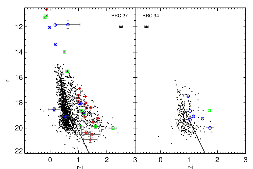
Figure 8: $r$ vs. $(r-i)$ color-magnitude diagram for BRC 27 (left) and BRC 34 (right). Note that these are AB magnitudes (not Vega magnitudes). No comparison to CG4+Sa101 or SWIRE is provided here, as optical color-magnitude diagrams are reasonably common. In each panel, small dots are objects in the catalog (i.e., objects seen in the image); green squares are literature high-confidence YSOs, red diamonds are literature candidate YSO, and blue circles are our new candidate YSOs presented here. Typical error bars are indicated below the BRC names in the plots – $\sim$0.06 mags in $r$ and $r-i$. Objects with exceptionally large error bars have error bars overplotted in grey. The solid black line is the main sequence relation from Bochanski et al. (2010), shifted to 1.2 kpc for BRC 27 and to 800 pc for BRC 34; the relation is not provided for $r-i<0.62$. Most of the YSOs and YSO candidates are in the location expected for confirmed YSOs. Two new YSO candidates in BRC 27 seem anomalously faint, as do three objects seen here only as limits; see text.

Optical photometric data can greatly aid in confirming or refuting YSO candidacy because they provide constraints on the Wien side of the SED. In Guieu et al. (2010), most of the IRAC-selected candidates in IC 2118 proved to be too faint, most vividly in the optical, to be likely cluster members. We obtained new optical data for our BRC 27 and 34 candidates as described in Section 3.3. An optical color-magnitude diagram for our regions and candidates appears in Figure 8; recall that these optical magnitudes are in the AB system rather than the Vega system. Few galaxies are expected to be detected in these bands; most of the objects seen here are stars, and most of the stars from the rest of the Milky Way Galaxy in the background will fall below the zero-age main sequence (ZAMS) placed at an appropriate distance for the BRCs we are considering. Legitimate young stars will be located above the ZAMS, but so will AGB star contaminants and foreground stars. Legitimate young stars may also suffer from reddening, which will slide the observed points back along a line roughly parallel to the ZAMS. Some legitimate young stars suffering very high extinction (notably edge-on disks where the detected optical light is primarily scattered light) may appear below the ZAMS (see, e.g., Rebull et al. 2010).

Most of the literature YSOs, literature YSO candidates, and new YSO candidates, at least those for which we have enough optical data to plot them in the Figure, are in the expected location in the optical CMD, meaning above the clump of objects in the rest of the Galaxy and above the ZAMS. Many of the objects that have IRAC measurements but were not selected as YSO candidates above (e.g., failing the Gutermuth-style color cuts in Section 4.1) also fall in the clump of objects from the rest of the Galaxy. The YSOs and candidate YSOs in BRC 27 between $r\sim 16$ and $\sim$20 that are above the ZAMS are even reasonably tightly correlated roughly along an isochrone (which is roughly parallel to the ZAMS), consistent with them all being members of a co-eval cluster (e.g., Orion in Rebull et al. 2000). It is not as strongly correlated, as expected, at the fainter end, because the photometry gets more uncertain. There are fewer objects in BRC 34, and they are less clearly clumped along an isochrone; this may be an indication that there are more contaminants in the BRC 34 sample, or there may be more of a range of apparent ages in this region.

Nine of the BRC 27 objects, candidates and known YSOs, are very bright, with $r\lesssim 16$. A common contaminant in these kinds of Spitzer-driven source selection is reddened background asymptotic giant branch (AGB) stars. None of the SEDs for these objects (see §5.3) resemble highly reddened objects, and they are not bright enough to be nearby AGB stars. The bright known YSOs or literature YSO candidates are of comparable brightness to the new bright YSO candidates, so the new objects are not distinctly different in optical properties. None of the BRC 34 objects are as bright as these brightest BRC 27 objects, despite the fact that BRC 34 is closer at $\sim$800 pc (vs. 1.2 kpc for BRC 27). Follow-up spectra are desirable, including line regions that can discriminate AGB stars from YSOs. These optically bright objects (also tagged in Table 3) are: 070353.5-112350 (=row 4), 070353.8-112341 (=row 6; this is the bright one with the large error in Figure 8), 070358.4-112325 (=row 10), 070401.3-112334 (=row 15), 070402.2-112542 (=row 19), 070402.3-112539 (=row 20), 070403.9-112609 (=row 25), 070406.0-112128 (=row 33), and 070408.0-112354 (=row 40).

Two of the new YSO candidate objects from BRC 27, 070401.6-112406 (=row 16) and 070406.5-112128 (=row 37), appear below the ZAMS in Figure 8. The latter has large enough errors that it could also be on (rather than below) the ZAMS, though even that would still set it apart from most of the rest of the YSOs and candidates in Figure 8. We examined the optical images for these objects, and both objects can clearly be seen in the images. However, 070406.5-112128 (=row 37) is near a brighter star such that it falls right on a diffraction spike. We have attempted to estimate the flux density despite the spike, but there is most likely a larger uncertainty on that measurement than we have estimated. Both SEDs are somewhat unusual (see Section 5.3.1 below, and Table 3), but they are located right on the bright rim of the BRC (Section 5.4). We have retained these in the list of YSO candidates under consideration although there is some uncertainty, in particular, for these objects.

One object from BRC 34 is on the ZAMS – 213323.8+580632 (=row 46). Notably, this object was one of the ones added based on the [3.6]$-$[8] color in Section 4.4, and was not automatically selected by the Gutermuth-style color cuts (Section 4.1). While this optical placement does not rule out the selection of this object as a YSO candidate, there is more uncertainty for this object than many of the rest of the YSO candidates in BRC 34.

As mentioned in Section 3.3 above, we sought out optical detections or limits for those objects on our list of new YSO candidates. Therefore, despite our optical completeness limits of $r\sim 20$, $i\sim 19$, some of the objects in Table 2 have optical detections fainter than this; each of those have been checked in the image. Many objects are too faint to be detected on the image, which may be an indication of embeddedness, or it may be an indication that the object is a contaminant. Those objects with high $A_{V}$ can be selected either from the shape of the SED (see §5.3), or from the near-IR, which we now discuss.

5.2 Near-IR Properties

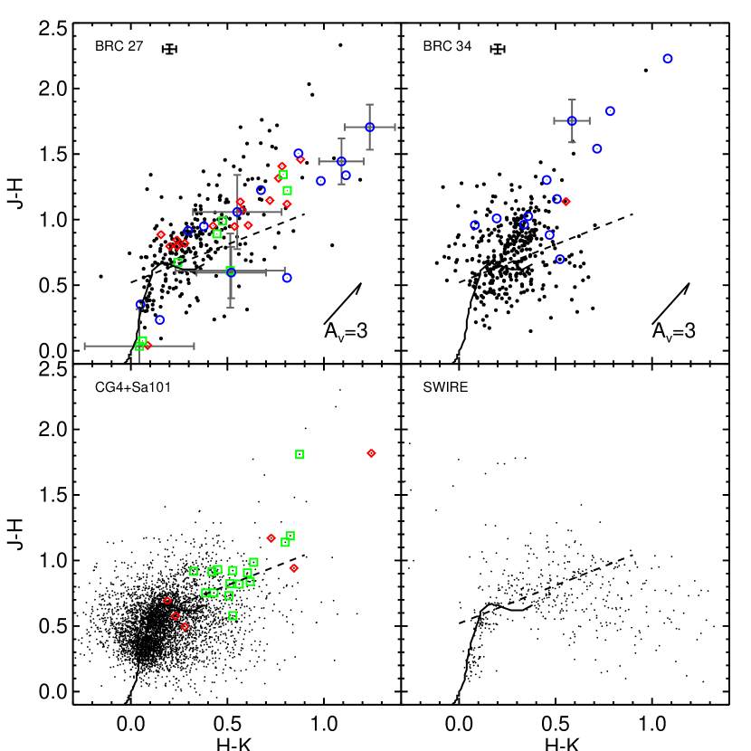
Figure 9: $J-H$ vs. $H-K_{s}$ color-color diagram for BRC 27 (upper left) and BRC 34 (upper right), with CG4+Sa101 (lower left) and SWIRE (lower right) for comparison. In each panel, small dots are objects in the catalog (i.e., objects seen in the image); green squares are literature high-confidence YSOs, red diamonds are literature candidate YSO, and blue circles are our new candidate YSOs presented here. Sample error bars are indicated just to the right of the BRC label in each of the BRC plots. Objects with exceptionally large error bars have error bars overplotted in grey. A sample $A_{V}$=3 (note not 30 as in the other plots) vector is included in the BRC 27 and 34 panels for reference. The ZAMS is indicated by a solid line, and the dashed line is the locus of dereddened young stars with a NIR excess from Meyer et al. (1997). Many of the known YSOs, literature YSO candidates, and new YSO candidates have a NIR excess starting at H-band with moderate reddening; see text for more discussion.

Near-IR photometric data can also aid in confirming or refuting YSO candidacy, through adding points to the SED and through location of the objects in the color-color diagram. Since we do not have spectral types for most of our sources, it is difficult to estimate the degree of reddening ($A_{V}$) uniquely for each object, but $JHK_{s}$ data can help us identify those objects with likely large $A_{V}$. Figure 9 shows $J-H$ vs. $H-K_{s}$ for the sample, with the data from CG4+Sa101 and SWIRE again included for comparison. Dust-free and reddening-free photospheres will follow the main sequence relation. SWIRE’s few stars cluster around the ZAMS relation; a large number of stars cluster around the ZAMS relation in CG4+Sa101. Because 2MASS is relatively shallow, relatively few galaxies are expected to be detected in the BRCs, though galaxies can appear in the same portion of the diagram as YSOs (as seen in the SWIRE panel of Fig. 9). Stars (or, indeed, any objects) that are simply reddened will be shifted along the reddening vector as indicated to the upper right; if the star has no NIR excess due to a circumstellar disk, an estimate of $A_{V}$ can be obtained by moving the object back along the reverse direction of the $A_{V}$ vector until intercepting the main sequence relation. However, there is a degeneracy in this process in that one can move the star back until it intercepts the low-mass portion of the ZAMS relation or the higher-mass portion, so a spectral classification is needed to obtain a good estimate of $A_{V}$. Moreover, stars with large NIR excesses due to circumstellar dust, when dereddened, cluster along a locus defined by Meyer et al. (1997), so objects with high $A_{V}$ as well as a NIR excess may not slide all the way back to the ZAMS relation.

Figure 9 suggests that many of our new YSO candidates have an infrared excess with a moderate degree of reddening. In BRC 27, 30 of the 38 shown here (82%) are above the locus from Meyer et al. (1997); in BRC 34, 12 of the 13 shown here (92%) are above the locus from Meyer et al. (1997). Far fewer objects in CG4+Sa101 (and essentially none in SWIRE) are subject to comparable levels of reddening.

The four most extreme red YSOs or candidate YSOs in BRC 34 are, in order from reddest to bluest, 213334.8+580409 (=row 51 in the Tables), 213340.8+580631 (=row 56), 213332.2+580558 (=row 50), and 213340.8+580626 (=row 55). These objects have $H-K_{s}>0.56$ and $J-H>1.2$. All four of these objects can be moved back to the main sequence relation without invoking an excess at $K_{s}$ band, and their SED shapes support this (Section 5.3). These are noted in Table 3.

In BRC 27, 14 YSOs or candidate YSOs have $H-K_{s}>0.6$ and $J-H>1.1$. The four reddest are 070400.7-112323 (=row 11), 070401.2-112242 (=row 13), 070401.6-112406 (=row 16), 070403.9-112326 (=row 26), all of which are new YSO candidates. The next ten are 070352.2-112100 (=row 1=Chauhan 109), 070353.2-112403 (=row 3=Ogura 3), 070401.2-112531 (=row 12), 070401.2-112233 (=row 14=Chauhan-anon), 070401.6-112132 (=row 17), 070402.1-112512 (=row 18), 070403.0-112350 (=row 23=Ogura 10=Chauhan 85), 070403.1-112327 (=row 24=Chauhan 107), 070405.1-112313 (=row 30=Ogura 15=Chauhan 88), and 070406.0-112315 (=row 34=Ogura 17=Chauhan 90). These are noted in Table 3. Most if not all of these can be moved back to the Meyer et al. (1997) locus before reaching the ZAMS relation, suggesting that most of them have an excess at $K_{s}$ band. Inspection of the SED shapes support this in many cases (Section 5.3.1).

At the blue end, none of the BRC 34 YSOs or candidate YSOs but up to five of the YSOs or candidate YSOs in BRC 27 are likely high-mass objects (B or A stars) with little or no $A_{V}$. These objects may have formed in or near BRC 27, or they may be foreground objects. The only two previously identified objects in BRC 27 that have spectral types are B and A stars, and are among these bluest objects. These bluest YSOs and YSO candidates are 070353.5-112350 (=row 4=Shevchenko 90, type A0), 070358.4-112325 (=row 10), 070402.3-112539 (=row 20=Shevchenko 99, Gregorio 75, type B3-5), 070403.9-112609 (=row 25=Shevchenko 102), and 070406.0-112128 (=row 33). These are also noted in Table 3.

5.3 Spectral Energy Distributions

Figure 10: Spectral Energy Distributions (SEDs) for the YSOs and YSO candidates discussed here. Units of $\lambda F_{\lambda}$ as presented are erg s^-1 cm^-2, and $\lambda$ is in microns. $+$ symbols are optical data from the literature, asterisks are our new optical data, diamonds are 2MASS (NIR) data, circles are IRAC data, and squares are MIPS data. Arrows are upper limits. The error bars (most frequently far smaller than the size of the symbol) are indicated at the center of the symbol. Catalog numbers appear in the upper left, row numbers (from the Tables) appear in the upper right, and a prior identification, if it exists, is in the lower left.

Figure 11: SEDs, continued. Notation as in previous figure.

Figure 12: SEDs, continued. Notation as in previous figure.

Figure 13: SEDs, continued. Notation as in previous figure.

Figure 14: SEDs, continued. Notation as in previous figure.

Figure 15: SEDs, continued. Notation as in previous figure.

Figure 16: SEDs, continued. Notation as in previous figure.

Table 4: Numbers and Fractions of YSO Classes in BRC 27 and BRC 34

type	BRC 27	BRC 34
Class I	3 (7%${}^{+6}_{-3}$)	1 (7%${}^{+13}_{-2}$)
Flat	7 (17%${}^{+7}_{-4}$)	1 (7%${}^{+13}_{-2}$)
Class II	23 (55%${}^{+7}_{-8}$)	8 (57%${}^{+11}_{-13}$)
Class III	9 (21%${}^{+8}_{-5}$)	4 (29%${}^{+14}_{-9}$)

5.3.1 Comments on Individual SEDs

Figures 10–16 are the SEDs for the YSOs and YSO candidates discussed here. All of the YSOs and YSO candidates have SEDs that resemble SEDs from other young stars (see, e.g., Rebull et al. 2010). We now highlight a few SEDs for discussion here; these notes are summarized in Table 3.

Three objects (070352.2-112100=Chauhan 109=row 1 in the Tables, 070354.6-112011=Chauhan 108=row 7, and 070403.1-112327=Chauhan 107=row 24) have literature optical points that are not consistent with the rest of the SED, including the optical data that we report here. While young stars are expected to vary in the optical, even if these are all legitimate young stars, the discrepancy is considerably larger than would be expected ($\sim$2 orders of magnitude in the SED). These optical data all come from Chauhan et al. (2009). Not all of the objects with data from Chauhan et al. (2009) are inconsistent with the rest of the respective SED, but all three of these are from Chauhan et al. (2009). As we note above in Section 2.2, extended emission near these objects can be seen in the 2MASS image, suggesting that perhaps the optical data from Chauhan et al. (2009) could have included some component due to extended emission.

One more source, 070401.3-112334 (=Gregorio 74, Chauhan-anon=row 15), has one optical data point (not from Chauhan et al. 2009 but from Gregorio-Hetem et al. 2009) that is not quite aligned with the rest of the SED. However, it is in the upper range of expected variability for young stars in the optical, and, since this $R$ photometry reported in Gregorio-Hetem et al. (2009) traces back to the USNO catalog from the digitization of the POSS (R) plates, uncertainties comparable to this are possible if not likely.

Four sources from the literature are identified in Section 4 above as not having significant excesses, and their SED shapes bear that out. Object 070352.7-112313 (=Ogura 2, Chauhan 81=row 2) and 070403.9-112609 (=Shevchenko 102=row 25) do not obviously have an IR excess. Object 070353.5-112350 (=Shevchenko 90=row 4) can be seen in the SED to be very bright; there might be a weak excess, though as the calculations above bear out, it is not very significant. Finally, object 070404.5-112555 (=Ogura 13=row 28) can be seen to have 5.8 and 8 $\mu$m points with considerably larger errors than are in the other SEDs, and a line through those points does not particularly smoothly join with the rest of the SED, consistent with the fact that these points are indeed quite uncertain. It could be that the 4.5 $\mu$m point is too low; however, the large errors on the longer wavelength points lead us to suspect that they are more likely to be in error.

One new YSO candidate in BRC 27 and four new YSO candidates in BRC 34 have SEDs very similar to 070404.5-112555 (=row 28) in that the 5.8 and 8 $\mu$m points abruptly rise in comparison to the 3.6 and 4.5 $\mu$m points; in each of these cases, it could be (also or instead) that the 4.5 $\mu$m point is too low. For object 070405.7-112123 (=row 31), the formal errors on the 5.8 and 8 $\mu$m are larger than usual, but not as large as 070404.5-112555 (=Ogura 13=row 28). The four similar objects from BRC 34 are 213314.5+580351 (=row 43), 213323.8+580632 (=row 46), 213336.2+580324 (=row 53), 213336.8+580329 (=row 54). All of these are not as discontinuous as 070404.5-112555 (=Ogura 13=row 28), and they do not have as large errors on 5.8 and 8 $\mu$m, but the SED shapes are similar.

Three more objects from BRC 27 have an abrupt rise in the longest wavelength point available, which could be indicative of a large inner disk hole. However, the spatial resolution at the longest bands is worse than at the shorter bands, and this longest wavelength point could be subject to contamination from the nebula or a nearby (in projection) background object. Object 070406.0-112128 (=row 33) and 070408.0-112354 (=Ogura 22, Chauhan 97=row 40) may have their 24 $\mu$m measurements contaminated; 070402.3-112539 (=Shevchenko 99, Gregorio 75=row 20) has no 24 $\mu$m data, but its 8 $\mu$m data may similarly be subject to contamination.

There is one last set of objects with abrupt changes between two points adjacent in wavelength. Objects 070407.9-112311 (=Ogura 21=row 39) and 070408.1-112309 (=Ogura 23, Chauhan 98=row 42) both have a discontinuity between $K_{s}$ and 3.6 $\mu$m. It is unclear what the physical origin of such a discontinuity might be, except for intrinsic stellar variations, and/or errors in the photometry.

Object 070353.8-112341 (=row 6) was mentioned above because it has no IRAC excess (§4.2), a marginal 24 $\mu$m excess (§4.3), and was bright in $r$ though with large errors (§5.1). The SED is consistent with all of these observations; the optical portion of the SED suggests that either there is a small $r$ excess, or that the measurement is in error by being too bright. It is unlikely that a YSO with such a small IR excess would be accreting at a high enough rate to affect $r$ via veiling. Multiband optical photometry (and spectroscopy, of course) will clarify what is going on with this object.

Two objects from BRC 27 were called out in Section 4.4 as having small excesses; their SEDs are consistent with that. They are 070354.9-112514 (=Ogura 5, Chauhan 94=row 8) and 070406.5-112227 (=row 36).

Two objects from BRC 27 and three from BRC 34 particularly seem, from their SEDs, to be subject to high $A_{V}$. All of them were also identified in Section 5.2 as having large $A_{V}$. They are 070400.7-112323 (=row 11), 070401.2-112233 (=Chauhan-anon=row 14), 213334.8+580409 (=row 51), 213340.8+580626 (=row 55), and 213340.8+580631 (=row 56).

Four YSOs and YSO candidates in BRC 27 and one in BRC 34 have SEDs characteristic of reasonably deeply embedded YSOs. They are object 070401.2-112242 (=row 13), 070402.7-112325 (=row 21), 070402.9-112337 (=Ogura 8+9, Chauhan 84=row 22), 070403.0-112350 (=Ogura 10, Chauhan 85=row 23), and (in BRC 34) 213332.2+580329 (=row 49). This last one in BRC 34 is the only object in either BRC detected at 70 $\mu$m, and it is very bright, with [70]$\sim-2$. We suspect that this will turn out to be a legitimate YSO and likely the youngest object of the ensemble we discuss here. It also seems to be centered within the globule of dust being illuminated to form the bright rimmed cloud (see Figure 4 or 18). It is also subject to so much reddening that there is no $J$ or $H$ detected for this object. Follow-up of this object will be difficult given the high $A_{V}$. The objects in BRC 27 have roughly similarly shaped SEDs. Object 070401.2-112242 (=row 13), a new YSO candidate, is not detected at $r$ or $i$ but does have $JHK_{s}$ measurements. Object 070402.7-112325 (=row 21), another new YSO candidate, is not detected at $r$, $i$, or $J$. Object 070402.9-112337 (=Ogura 8+9, Chauhan 84=row 22) is a literature YSO candidate consisting of two sources unresolved in the 2MASS and IRAC data. This one is detected at the optical and NIR bands, but the overall SED shape is roughly similar to the others. Object 070403.0-112350 (=Ogura 10, Chauhan 85=row 23), similarly, is detected at the optical and NIR bands.

Somewhat similarly to the objects in the prior paragraph, 070403.9-112326 (=row 26) seems to have a substantial IR excess, and is not detected in the optical. It is possible in this case that are are detecting photosphere at $JHK_{s}[3.6]$, but if that were the case, substantial extinction would be needed. It could be a nearly edge-on disk seen mostly in scattered light at the shorter bands. However, this SED is also consistent with an background galaxy subject to extinction. Follow-up spectra would be very helpful in determining the nature of this object.

Three SEDs are somewhat unusually shaped. Objects 070401.6-112406 (=row 16), 070402.2-112542 (=row 19), and 070406.5-112128 (=row 37) are all new YSO candidates from BRC 37. Two of them, 070401.6-112406 (=row 16) and 070406.5-112128 (=row 37), have optical detections that place them below the ZAMS (Section 5.1), but they are located right on the bright rim itself (Section 5.4), a suggestive location for young stars. Object 070401.6-112406 (=row 16) is a more or less steadily rising SED, which could be a background galaxy subject to extinction, or a YSO. This object also, in the $J$ through [4.5] images, has nearby emission that could be from the nebula or could be from nearby point sources. The morphology of the emission around this source is complex, particularly in the [3.6] and [4.5] bands, where there seems to be a mixture of point and extended emission within 2-10$\arcsec$; higher spatial resolution observations would be very useful for this object. In contrast to 070401.6-112406 (=row 16), 070402.2-112542 (=row 19) is bright in $r$ (Section 5.1). It has a point at 8 $\mu$m that is higher than the 5.8 and 24 $\mu$m points in the SED, very suggestive of PAH emission that could be a background galaxy (see “8 micron pop-ups” in Rebull et al. 2010), but it could also be a young star. It is very bright in the image, though fainter than another nearby bright star (070402.3-112539=Shevchenko 99, Gregorio 75=row 20), so photometry is difficult. This object may be a legitimate infrared-bright companion to this bright object (like in WL 20, Ressler & Barsony 2001). Follow-up observations are warranted.

All the rest of the YSOs and YSO candidates have SEDs that are completely consistent with young stars having IR excesses, but not deserving of special comment here.

5.3.2 SED Classifications

Following the discussion in Section 2.1, in the spirit of Wilking et al. (2001; see also Lada & Wilking 1984, Lada 1987, Greene et al. 1994, and Bachiller 1996), we define the near- to mid-IR (2 to 24 $\mu$m) slope of the SED, $\alpha=d\log\lambda F_{\lambda}/d\log\lambda$, where $\alpha>0.3$ for a Class I, 0.3 to $-$0.3 for a flat-spectrum source, $-$0.3 to $-$1.6 for a Class II, and $<-$1.6 for a Class III. For each of the YSOs and candidate YSOs in our sample, we performed a simple ordinary least squares linear fit to all available photometry (just detections, not including upper or lower limits) as observed between 2 and 24 $\mu$m, inclusive. Note that: (a) the formal errors on the infrared points are so small as to not affect the fitted SED slope; (b) the fit is performed on the observed SED, meaning that no reddening corrections are applied to the observed photometry before fitting; (c) the fit is performed on the observed SED, meaning that if there is no 24 $\mu$m data point, then that point is necessarily not included in the fit. In the literature, the precise definition of $\alpha$ can vary, which may result in different classifications for certain objects. Classification via this method is provided specifically to enable comparison within this paper (and to CG4+Sa101) via internally consistent means. Note that the formal classification puts no lower limit on the colors of Class III objects (thereby including those with SEDs resembling bare stellar photospheres, and allowing for other criteria to define youth). By searching for IR excesses, we are incomplete in our sample of Class III objects. The SED slopes and classes for the YSO and YSO candidates discussed here appear in Table 3.

Of all the evolutionary stages of YSOs among the YSOs or YSO candidates discussed here, Class I is the shortest lived, and therefore the rarest of all the SED classes. There are four objects, all new YSO candidates, that have an SED class of I. Three of these objects are in BRC 27, and one is in BRC 34. Of the three objects in BRC 27, two are possible (if not likely) background objects (see Section 5.3.1); these are 070401.6-112406 (=row 16) and 070406.5-112128 (=row 37), and they are the ones below the main sequence in Figure 8 (and Section 5.1. The other two new Class I candidates are 070403.9-112326 (=row 26) and 213332.2+580329 (=row 49), the latter of which is the bright source seen at [70] in BRC 34.

Several objects are on the borderline between SED classes, meaning that their fitted SED slope is within 0.1 of the dividing line between the classes as defined just above. These objects may be members of adjacent classes at a different inclination (see discussion above in Section 2.1); the addition of a new point at 24 $\mu$m (or a new detection where any source confusion is resolved) may also change the classification of some of these objects. There are six of these borderline objects in BRC 27: 070403.9-112326 (=row 26, on the borderline between Class I and Flat), 070401.7-112323 (=row 11, on the borderline between Flat and Class II; in this case, a different [24] could make a big difference), 070405.1-112313 (=row 30=Ogura 15, Chauhan 88, on the borderline between Flat and Class II), 070404.5-112555 (=row 28=Ogura 13, on the borderline between Class II and III; we have tagged this one as not having an IR excess due to the uncertainty of the 5.8 and 8 $\mu$m points, so this ends up as a Class II [rather than a III] with no excess), 070406.4-112336 (=row 35=Ogura 18, Chauhan 91, on the borderline between Class II and III), and 070408.1-112313 (=row 41, on the borderline between Class II and III). In BRC 34, there are four borderline objects: 213336.2+580324 (=row 53, on the borderline between Flat and Class II), and the remaining three are all on the borderline between Class II and III: 213314.5+580351 (=row 43), 213319.4+580406 (=row 45, and in this case a different measurement at [8] might directly impact the slope), and 213335.3+580647 (=row 52). When the SED slope fit is formally made to all available measurements between 2 and 8 $\mu$m, rather than all available points between 2 and 24 $\mu$m, the slopes change enough to change the classifications for just 6 of the 56 total objects (11%) considered here (out of the 19 with 24 $\mu$mdetections, 32%), all of which are in BRC 27, and none of which are listed as borderline cases above. These are: 070401.2-112242 (=row 13, which changes from a Flat to Class II), 070402.2-112542 (=row 19, which changes from a Flat to Class I) 070402.9-112337 (=row 22=Ogura 8+9=Chauhan 84, which changes from a Flat to Class II) 070406.0-112128 (=row 33, which changes from a Class II to Class III) 070406.0-112315 (=row 34=Ogura 17=Chauhan 90, which changes from a Flat to Class II) 070408.0-112354 (=row 40=Ogura 22=Chauhan 97, which changes from a Class II to Class III).

Taking all of the slopes and classifications at face value, Table 4 summarizes the fraction of Class I, Flat, Class IIs and Class IIIs (such as we know them) for each of the two BRCs. The errors on these disk fractions as tabulated in Table 4 were calculated using the binomial distribution, as per Burgasser et al. (2003). The largest calculated fraction of objects in BRC 27 is Class II, at $\sim$55%. The largest fraction of objects in BRC 34 is also Class II objects, at a quite comparable $\sim$57%, but with so many fewer YSOs in BRC 34, the uncertainty on this fraction is larger than for BRC 27. For both BRCs, the next largest fraction of objects is Class III, at 21% and 29% for BRC 27 and 34, respectively. These are consistent with each other within the errors, and also certainly our sample of Class III objects is incomplete in both BRCs. The fraction of Class I+Flat spectrum objects in BRC 27 (10/42, or 24%; incorporating errors, this value could be between 19 and 31%) is consistent within errors with that for BRC 34 (2/14, or 14%, incorporating errors, this value could be between 9 and 28%). It is very difficult to draw any conclusions about relative ages of the two BRCs. They are identical within small-number statistics; moreover our samples are incomplete, and include unconfirmed YSOs. Further spectroscopy is desirable.

In CG4+Sa101, there are only 7 YSOs or YSO candidates near the BRC itself (CG4); there are 15 more nominally associated with Sa101. Considering the ensemble of objects in CG4+Sa101, 73% (incorporating errors, this value could be between 62%-80%) are Class II objects; for just CG4, 71% (incorporating errors, this value could be between 51%-82%) are Class II objects. For either sample, this is a slightly larger fraction than found in either BRC 27 or BRC 34, suggesting that CG4+Sa101 could be slightly older.

5.4 Location on the Sky

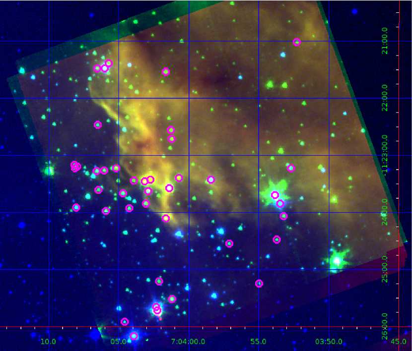
Figure 17: Three-color image of BRC 27 (blue=$i$, green=3.6 $\mu$m, red=8 $\mu$m). The YSOs (known and candidate) are indicated by additional magenta circles. North is up, and coordinates are indicated. Young stars are statistically more likely to be clustered, and associated with the nebulosity, than background or foreground contaminants.

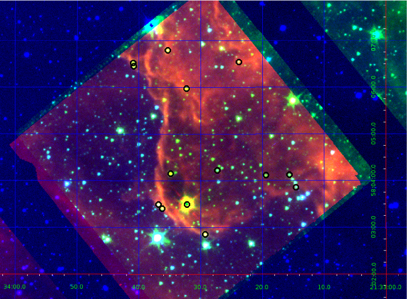
Figure 18: Three-color image of BRC 34 (blue=$i$, green=3.6 $\mu$m, red=8 $\mu$m). The YSOs (known and candidate) are indicated by additional black circles. North is up, and coordinates are indicated. Young stars are statistically more likely to be clustered, and associated with the nebulosity, than background or foreground contaminants.

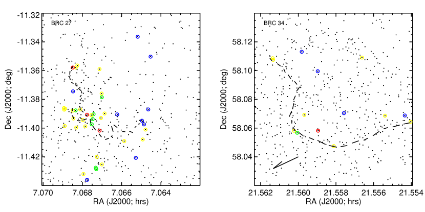
Figure 19: Positions of the objects in both BRCs on the sky, color-coded by shape of the SED – blue is Class III, green is Class II, yellow is Flat, and red is Class I. Small black dots are objects in the 2MASS point source catalog. the black dashed lines are the approximate edges of the BRC, as seen in Figure 17 and 18. While the source of the shock front is uncertain for BRC 27, it is probably to the Southeast. The source is known for BRC 34; the source (HD 206267) is about a degree away in the direction of the arrow as shown. There is some evidence in the literature that more embedded objects (earlier classes) should be further from the exciting source. There are too few sources here to assess this.

Figure 17 and 18 both show 3-color images with the selected set of YSOs indicated. Young stars are statistically more likely to be clustered, and associated with the nebulosity, than background or foreground contaminants. Certainly, this is not a strict rule; young stars can appear off the cloud and contaminants can be seen through the cloud, superimposed on the cloud, and/or be clustered.

Figure 19 shows the position of the objects with color coding corresponding to the shape of the SED. The source of the shock front is not known in BRC 27, but it probably to the Southeast, given the shape of the nebula. The source of the shock is known in BRC 34 to be HD 206267, which is about a degree away, also to the Southeast. The eponymous “bright rim” is more obvious in the MIR in BRC 34 than BRC 27. The rim of BRC 27 is less well-defined and has more texture in the images, perhaps indicating the effects of more than one exciting OB star, or a distribution of densities in the molecular matter composing the BRC.

In BRC 27, there are 3 times more objects than BRC 34, with a YSO surface density of $\sim$1.7 objects arcmin^-1, as compared with $\sim$0.6 objects arcmin^-1 in BRC 34. In BRC 27, there seems to be a cluster of objects just off the dark cloud, near $(\alpha,\delta)$=(106.02$\arcdeg$, $-$11.40$\arcdeg$)=(07^h05^m, $-$11$\arcdeg$23$\arcmin$05$\arcsec$). They may have been recently revealed by the action of the shock front; they are largely Class II objects, consistent with this idea, but not conclusive proof of it. All of the Class I candidate objects are on or behind the bright rim, again consistent with (but not proof) that younger objects are found within the dark cloud. If the shock front is triggering star formation in the clump, one might expect that all of the Class I objects would be deep inside the cloud, with the least embedded objects having been revealed by the ionization front in front of the cloud. Both clouds have Class III objects projected onto the cloud, though the Class III objects are the least complete sample and most uncertain membership. In BRC 34, many of the YSOs are along the bright rim itself, whereas in BRC 27, they are more dispersed with respect to the distribution of bright ISM, with more YSOs or candidates off the dark cloud, on the excitation side of the bright rim. If this is, in both cases, a wave of star formation that moves through the BRC, this would be consistent with BRC 27 being slightly older than BRC 34. However, with so few objects, and with the various uncertainties that have gone into selecting our sample, we cannot make any clear statements about whether there is, in fact, an age gradient through the BRCs, or evidence for small-scale sequential star formation.

In CG4+Sa101, the YSOs or candidate YSOs formally associated with Sa101 are relatively tightly clustered, with a median nearest neighbor distance of 62$\arcsec$; in the CG4 subregion, the median nearest neighbor distance is five times larger. A similar kind of calculation in the BRCs is more difficult, because the maps are so much smaller, and because there is not as obvious a clumping in the image. For both BRCs, the median nearest neighbor distance is $\sim$10$\arcsec$. Limiting this calculation to just the clump of objects in BRC 27 between 7.0665 and 7.069 hrs of RA and $-$11.38 and $-$11.40 deg of Dec obtains approximately the same median separation, presumably because this clump dominates the statistics. Surveys of a larger region around these BRCs will help reveal any clustering.

6 Conclusions

We used Spitzer Space Telescope data from the Spitzer Heritage Archive to search for new candidate young stars in two BRC regions, BRC 27 (part of CMa R1) and BRC 34 (part of the IC 1396 complex). These regions both appear to be actively forming young stars, perhaps triggered by the proximate OB stars.

We have presented Spitzer and optical data for 42 YSOs, literature YSO candidates, and new YSO candidates in BRC 27. Out of those, we identify 22 of the 26 literature YSOs or literature YSO candidates as having an IR excess, though one of them has an uncertain IR excess. There are 16 new YSO candidates that we have identified from their Spitzer colors, although 3 of them have somewhat uncertain IR excesses.

Similarly, we have presented Spitzer and optical data for 14 YSO candidates (including one known YSO) in BRC 34. The one known YSO in BRC 34 has a clear IR excess, and there are 13 additional new objects we have identified as candidate YSOs from their Spitzer colors. Of those 13, 3 have somewhat uncertain IR excesses; one is a likely Class I and is the only 70 $\mu$m point source detection in either BRC.

As far as we can determine, these objects have properties in the optical, NIR, and MIR that suggest that they are YSOs. However, follow-up spectroscopy is needed to affirm or refute their YSO status.

Assuming that these YSO candidates are all legitimate YSOs, in BRC 27, there are 3 times more objects than BRC 34, with a YSO surface density of $\sim$1.7 objects arcmin^-1, as compared with $\sim$0.6 objects arcmin^-1 in BRC 34. Considering the entire ensemble, both BRCs are likely of comparable ages, based primarily on SED class ratios. Within small-number statistics, and the fact that our samples are probably incomplete and include unconfirmed YSOs, no definitive statement can be made about the relative ages of the ensemble of YSOs in these BRCs. However, they both seem to have more objects at an earlier evolutionary stage than another BRC, CG4+Sa101 (BRC 48). Similarly, no clear conclusions can be drawn about any possible age gradients that may be present.

We plan to continue this project using Wide-field Infrared Survey Explorer (WISE; Wright et al. 2010) to investigate the YSO surface density in a wider area around these BRCs, as well as pursue follow-up spectroscopy.

References

- Abazajian et al. (2009) Abanzajian, K., et al., 2009, ApJS, 182, 543
- Allen et al. (2011) Allen L., et al. 2011, American Astronomical Society, BAAS, 43, 258.15.
- Allen et al. (2004) Allen, L. E., Calvet, N., D’Alessio, P., Merin, B., Hartmann, L., Megeath, S. T., Gutermuth, R., Muzerolle, J., Pipher, J., Myers, P., Fazio, G. 2004, ApJS, 154, 363
- Apai et al. (2005) Apai, D., et al., Science, 310, 834
- Bachiller (1996) Bachiller, R., 1996, ARA&A, 34, 111
- Balog et al. (2007) Balog, Z., et al., 2007, ApJ, 660, 1532
- Barrado & Martin (2003) Barrado y Navascués, D., & Martín, E., 2003, AJ, 126, 2997
- Beichman et al. (1998) Beichman, C. A., Neugebauer, G., Habing, H., Clegg, P., Chester, T. 1998, IRAS catalog and explanatory supplement
- Blum et al. (2006) Blum, R., et al., 2006, AJ, 132, 2034
- Bochanski et al. (2010) Bochanski, J. et al., 2010, AH, 139, 2679
- Burgasser et al. (2003) Burgasser, A. J., Kirkpatrick, J. D., Reid, I. N., Brown, M. E., Miskey, C. L., & Gizis, J. E. 2003, ApJ, 586, 512
- Chauhan et al. (2008) Chauhan N., Pandey A.K., Ogura K., Ojha D.K., Bhatt B.C., Ghosh S.K., Rawat, P.S., 2009, MNRAS, 396, 964
- Choudhury et al. (2010) Choudhury, R., Mookerjea, B., Bhatt, H., 2010, ApJ, 717, 1067
- Currie & Kenyon (2009) Currie, T., & Kenyon, S., 2009, AJ, 138, 703
- Engelbracht et al. (2007) Engelbracht, C., Blaylock, M., Su, K. Y. L., et al. 2007, PASP, 119, 994
- Evans et al. (2003) Evans, N., et al. 2003, PASP, 115, 965
- Evans et al. (2009) Evans, N., Dunham, M., Joergensen, J., et al. 2009a, ApJS, 181, 321
- Evans et al. (2009b) Evans, N., et al., 2009b, arXiv:0901.1691
- Fazio et al. (2004) Fazio, G., Hora, J. L., Allen, L. E., et al. 2004, ApJS, 154, 10
- Finkbeiner et al. (2004) Finkbeiner, D., et al., 2004, AJ, 128, 2577
- Gautier et al. (2007) Gautier, T. N., Rieke, G. H., Stansberry, J., 2007, ApJ, 667, 527
- Gordon et al. (2005) Gordon, K., Rieke, G., Engelbracht, C., et al. 2005, PASP, 117, 503