Sample Size Planning for Classification Models

Abstract

In biospectroscopy, suitably annotated and statistically independent samples (e. g. patients, batches, etc.) for classifier training and testing are scarce and costly. Learning curves show the model performance as function of the training sample size and can help to determine the sample size needed to train good classifiers. However, building a good model is actually not enough: the performance must also be proven. We discuss learning curves for typical small sample size situations with 5 – 25 independent samples per class. Although the classification models achieve acceptable performance, the learning curve can be completely masked by the random testing uncertainty due to the equally limited test sample size. In consequence, we determine test sample sizes necessary to achieve reasonable precision in the validation and find that 75 – 100 samples will usually be needed to test a good but not perfect classifier. Such a data set will then allow refined sample size planning on the basis of the achieved performance. We also demonstrate how to calculate necessary sample sizes in order to show the superiority of one classifier over another: this often requires hundreds of statistically independent test samples or is even theoretically impossible. We demonstrate our findings with a data set of ca. 2550 Raman spectra of single cells (five classes: erythrocytes, leukocytes and three tumour cell lines BT-20, MCF-7 and OCI-AML3) as well as by an extensive simulation that allows precise determination of the actual performance of the models in question.

1 Introduction

Sample size planning is an important aspect in the design of experiments. While this study explicitly targets sample size planning in the context of biospectroscopic classification, the ideas and conclusions apply to a much wider range of applications. Biospectroscopy suffers from extreme scarcity of statistically independent samples, but small sample size problems are common also in many other fields of application.

In the context of biospectroscopic studies, suitably annotated and statistically independent samples for classifier training and validation frequently are rare and costly. Moreover, the classification problems are often rather ill-posed (e. g. diseased vs. non-diseased). In these situations, particular classes are extremely rare, and/or large sample sizes are necessary to cover classes that are rather ill-defined like “not this disease” or “out of specification”. In addition, ethical considerations often restrict the studied number of patients or animals.

Even though the data sets often consist of thousands of spectra, the statistically relevant number of independent cases is often extremely small due to “hierarchical” structure of the biospectroscopic data sets: many spectra are taken of the same specimen, and possibly multiple specimen of the same patient are available. Or, many spectra are taken of each cell, and a number of cells is measured for each cultivation batch, etc. In these situations, the number of statistically independent cases is given by the sample size on the highest level of the data hierarchy, i. e. patients or cell culture batches. All these reasons together lead to sample sizes that are typically in the order of magnitude between 5 and 25 statistically independent cases per class.

Learning curves describe the development of the performance of chemometric models as function of the training sample size. The true performance depends on the difficulty of the task at hand and must therefore be measured by preliminary experiments. Estimation of necessary sample sizes for medical classification has been done based on learning curves [1, 2] as well as on model based considerations [3, 4]. In pattern recognition, necessary training sample sizes have been discussed for a long time (e. g. [5, 6, 7]).

However, building a good model is not enough: the quality of the model needs to be demonstrated.

One may think of training a classifier as the process of measuring the model parameters (coefficients etc.). Likewise, testing a classifier can be described as a measurement of the model performance. Like other measured values, both the parameters of the model and the observed performance are subject to systematic (bias) and random (variance) uncertainty.

(a) confusion matrix

(b) $\operatorname{Sens}_{A}$

(c) $\operatorname{Spec}_{A}$

(d) $\operatorname{PPV}_{A}$

(e) $\operatorname{NPV}_{A}$

Figure 1: Confusion matrix LABEL:sub@fig:Z and characteristic fractions LABEL:sub@fig:sens – LABEL:sub@fig:npv. The parts of the confusion matrix summed as enumerator and denominator for the respective fraction with respect to class $A$ are shaded.

Classifier performance is often expressed in fractions of test cases, counted from different parts of the confusion matrix, see fig. 1. These ratios summarize characteristic aspects of performance like sensitivity (Sens_A: “How well does the model recognize truly diseased samples?”, fig. 1b), specificity (Spec_A: “How well does the classifier recognize the absence of the disease?”, fig. 1c), positive and negative predictive values (PPV_A/NPV_A: “Given the classifier diagnoses disease/non-disease, what is the probability that this is true?”, fig. 1d and 1e). Sometimes further ratios, e. g. the overall fraction of correct predictions or misclassifications, are used.

The predictive values, while obviously of more interest to the user of a classifier than sensitivity and specificity, cannot be calculated without knowing the relative frequencies (prior probabilities) of the classes.

From the sample size point of view, one important difference between these different ratios is the number of test cases $n_{test}$ that appears in the denominator. This test sample size plays a crucial role in determining the random uncertainty of the observed performance $\hat{p}$, (see below). Particularly in multi-class problems, this test sample size varies widely: the number of test cases truly belonging to the different classes may differ, leading to different and rather small test sample sizes for determining the sensitivity $p$ of the different classes. On contrast, the overall fraction of correct or misclassified samples use all tested samples in the denominator.

The specificity is calculated from all samples that truly do not belong to the particular class (fig. 1c). Compared to the sensitivities, the test sample size in the denominator of the specificities is therefore usually larger and the performance estimate more precise (with the exception of binary classification, where the specificity of one class is the sensitivity of the other). Thus small sample size problems in the context of measuring classifier performance are better illustrated with sensitivities. It should also be kept in mind that the specificity often corresponds to an ill-posed question: “Not class A” may be anything. Yet not all possibilities of a sample truly not belonging to class A are of the same interest. In multi-class set-ups, the specificity will often pool easy distinctions with more difficult differential diagnoses. In our application [8, 9], the specificity for recognizing a cell does not come from the BT-20 cell line pools e. g. the fact that it is not an erythrocyte (which can easily be determined by eye without any need for chemometric analysis) with the fact that it does not come from the MCF-7 cell line, which is far more similar (yet from a clinical point of view possibly of low interest as both are breast cancer cell lines) and the clinically important fact that it does not belong to the OCI-AML3 leukemia. This pooling of all other classes has important consequences. Increasing numbers of test cases in easily distinguished classes (erythrocytes) will lead to improved specificities without any improvement for the clinically relevant differential diagnoses. Also, it must be kept in mind that random predictions (guessing) already lead to specificities that seem to be very good. For our real data set with five different classes, guessing yields specificities between 0.77 and 0.85. Reported sensitivities should also be read in relation to guessing performance, but neglecting to do so will not cause an intuitive overestimation of the prediction quality: guessing sensitivities are around 0.20 in our five-class problem.

Examining the non-diagonal parts of the confusion table instead of specificities avoids these problems. If reported as fractions of test cases truly belonging to that class, then all elements of the confusion table behave like the sensitivities on the diagonal, if reported as fractions of cases predicted to belong to that class, the entries behave like the positive predictive values (again on the diagonal).

Literature guidance on how to obtain low total uncertainty and how to validate different aspects of model performance is available [10, 11, 12, 13, 14]. In classifier testing, usually several assumptions are implicitly made which are closely related to the behaviour of the performance measurements in terms of systematic and random uncertainty.

Classification tests are usually described as Bernoulli-process (repeated coin throwing, following a binomial distribution): $n_{test}$ samples are tested, and thereof $k$ successes (or errors) are observed. The true performance of the model is $p$, and its point estimate is

$$\hat{p}=\frac{k}{n_{test}}$$ (1)

with variance

$$\operatorname{Var}\left(\frac{k}{n_{test}}\right)=\frac{p(1-p)}{n_{test}}$$ (2)

In small sample size situations, resampling strategies like the bootstrap or repeated/iterated $k$-fold cross validation are most appropriate. These strategies estimate the performance by setting aside a (small) part of the samples for independent testing and building a model without these samples, the surrogate model. The surrogate model is then tested with the remaining samples. The test results are refined by repeating/iterating this procedure a number of times. Usually, the average performance over all surrogate models is reported. This is an unbiased estimate of the performance of models with the same training sample size as the surrogate models [11, 1]. Note that the observed variance over the surrogate models possibly underestimates the true variance of the performance of models trained with $n_{train}$ training cases [1]. This is intuitively clear if one thinks of a situation where the surrogate models are perfectly stable, i. e. different surrogate models yield the same prediction for any given case. No variance is observed between different iterations of a $k$-fold cross validation. Yet, the observed performance is still subject to the random uncertainty due to the finite test sample size of the underlying Bernoulli process.

Usually, the performance measured with the surrogate models is used as approximation of the performance of a model trained with all samples, the final model. The underlying assumption is that setting aside of the surrogate test data does not affect the model performance. In other words, the learning curve is assumed to be flat between the training sample size of the surrogate model and training sample size of the final model. The violation of this assumption causes the well-known pessimistic bias of resampling based validation schemes.

The results of testing many surrogate models are usually pooled. Strictly speaking, pooling is allowed only if the distributions of the pooled variables are equal. The description of the testing procedure as Bernoulli process allows pooling if the surrogate models have equal true performance $p$. In other words, if the predictions of the models are stable with respect to perturbed training sets, i. e. if exchanging of a few samples does not lead to changes in the prediction. Consequently, model instability causes additional variance in the measured performance.

Here, we discuss the implications of these two aspects of sample size planning with a Raman-spectroscopic five-class classification problem: the recognition of five different cell types that can be present in blood. In addition to the measured data set, the results are complemented by a simulation which allows arbitrary test precision.

2 Materials and Methods

class	cell type	nspectra	sensitivity
			sim. LDA	sim. PLS-LDA	real PLS-LDA	real PLS-LDA batch-wise
rbc	erythrocytes	372	1.00	1.00	0.99 (0.96 – 0.99)	0.97 (0.96 – 0.98)
leu	leukocytes	569	1.00	0.99	0.97 (0.96 – 0.97)	0.87 (0.84 – 0.90)
mcf	MCF-7 breast carc.	558	0.95	0.87	0.91 (0.90 – 0.92)	0.31 (0.24 – 0.42)
bt	BT 20 breast carc.	532	0.91	0.72	0.75 (0.74 – 0.76)	0.38 (0.32 – 0.45)
oci	OCI-AML3 leukemia	518	0.94	0.86	0.89 (0.88 – 0.90)	0.30 (0.23 – 0.17)

Table 1: Data set characteristics: classes, number of spectra per class and “best possible” sensitivities. For the simulated (sim.) data (column “sim. LDA” and “sim. PLS-LDA”), $n_{test}$ = 2 $\cdot$ 10⁴ spectra. Best possible performance of the real data was estimated using 100$\times$ 5-fold cross validation, shown are average and 5^th to 95^th percentile of observed sensitivities over the iterations. Column “real PLS-LDA” corresponds to the setup for this study, treating each spectrum as independent of the other spectra, for column 7 (“real PLS-LDA batch-wise”) the validation splits patients and batches rather than spectra.

2.1 Raman Spectra of Single Cells

Raman spectra of five different types of cells that could be present in blood are used in this study. Details of the preparation, measurements and the application have been published previously [8, 9]. The data were measured in a stratified manner, specifying roughly equal numbers of cells per class beforehand, and do not reflect relative frequencies of the different cells in a target patient population. Thus, we cannot calculate predictive values for our classifiers.

For this study, the spectra were imported into R [15] using package hyperSpec [16]. In order to correct for deviations of the wavenumber calibration the maximum of the CaF2 band was aligned to 322 cm^-1. The spectra then underwent a smoothing interpolation (spc.loess) onto a common wavenumber axis ranging from 500 to 1800 and 2600 to 3200 cm^-1 with data point spacing of 4 cm^-1. Baseline correction was performed in the high wavenumber region by a third order polynomial fit to spectral regions where no CH stretching signals occur (2700 – 2825, 3020 – 3040 and 3085 – 3200  cm^-1) which was then used as baseline for the CH stretching bands from 2810 to 3085  cm^-1. A third order polynomial automatically selecting support points between 500 – 1200  cm^-1 was blended smoothly with a quadratic polynomial in the spectral range automatically selecting support points between 800 – 1200 and 1700 – 1800  cm^-1. After baseline correction, the spectral ranges 600 – 1800 and 2810 – 3085  cm^-1 were retained. Finally, the spectra were area normalized.

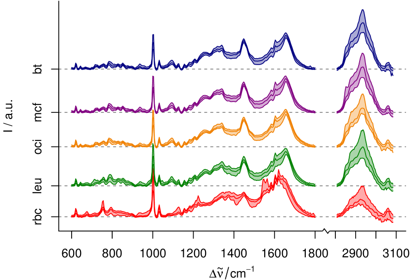
Figure 2: Spectra of the 5 classes: BT-20 breast carcinoma cells, MCF-7 breast carcinoma cells, OCI-AML3 leukemia cells, normal leukocytes and normal erythrocytes (from top to bottom). Shown are the median and the 5^th to 95^th percentile spectra. The confusion tables are available as supplementary material.

Figure 2 shows the preprocessed spectra. Erythrocyte (red blood cells, rbc) spectra can easily be recognized by the resonance enhanced characteristic signature of hemoglobin around 1600  cm^-1. Leukocyte (leu) spectra are rather similar to the tumour cell spectra, yet there are subtle differences in the shape of the CH2-deformation vibrations around 1440  cm^-1, the intensity of the $\nu_{CH}$ stretching vibrations (2810 – 3085  cm^-1) which are more intense in the tumour cells, and the intensity of the phenylalanine band at 1002  cm^-1 (less intense in the tumour cells). Between the different tumour cell lines (bt, mcf, and oci) no distinct marker bands are visible by eye.

Variation in the data set is introduced by using cells from 5 different donors (leukocytes and erythrocytes) and 5 different cultivation batches, respectively; measuring the cells on the first day of preparation and one day after (yielding 9 measurement days) and using two different lasers of the same model from the same manufacturer. For the present study, we pretend not to know of these influencing factors and treat the spectra as independent. This allows us to pretend that we have a sufficiently large data set to run reference calculations that can be used as ground truth. The consequence is that no performance for the recognition of the cell lines in general can be inferred from this study: the results would be heavily overoptimistic (tab. 1, see also [14] for a discussion of representative testing).

Hence, we have a data set of about 2500 spectra (tab. 1) of five classes with “unknown” influencing factors. The difficulty in recognising the five different classes varies widely: while erythrocytes are extemely easy to recognize, we expect that perfect recognition of leukocytes is possible as well though we expect that more training cases are needed to achieve this. Differential diagnosis of the cancer cell lines is more difficult, and substantial overlap between the two breast carcinoma cell lines BT-20 and MCF-7 has been observed in previous studies [8, 9]. Throughout this paper, we discuss the sensitivities for erythrocytes (rbc), leukocytes (leu) and the tumour cell line BT-20 (bt).

Of these 2500 spectra, we draw data sets of size 25 cases / class keeping the remaining spectra as a large test set to get a more precise estimate of the performance of the respective models.

rbc is the smallest class, its sensitivity can be estimated with a precision better than $\pm$ 0.052 (95 % confidence interval at sensitivity of 0.5).

2.2 Simulated Spectra

In addition to the experimental data set, simulations were used. This allows to study an idealized situation: arbitrarily large test sets allow to measure the true performance with negligible random uncertainty due to the testing. Thus, the random uncertainty due to model instability can be measured with the simulations while these two sources of random uncertainty cannot be separated for the real data.

For each of the five classes in the experimental data set, average spectrum and covariance matrix were calculated. Multivariate normally distributed simulated spectra were simulated using rmvnorm [17, 18]. Briefly, the Mersenne-Twister algorithm generates uniformly distributed pseudo-random numbers which are then converted to normally distributed random numbers via the inverse cumulative distribution function. The requested covariance structure is obtained by multiplying with the matrix root of the covariance matrix (calculated via eigenvalue decomposition) and the requested mean spectrum is added.

100 “small” data sets of 25 spectra / class (i. e. 125 spectra of all classes together per small dataset) were generated. For determining the real performance of the models, a large test set of 4 $\cdot$ 10⁴ spectra / class was generated. This means that the sensitivities can be measured with a precision of better than 0.5 $\pm$ 0.005 (95 % c.i.), the standard deviation of observed performance is then $\sigma(\hat{p})=\sqrt{\frac{p(1-p)}{n}}\leq\frac{0.5}{\sqrt{n}}=0.0025$.

In addition, one large training set of 2 $\cdot$ 10⁴ spectra / class was generated. This data set was used to estimate the best possible performance that can be obtained with the chosen classifiers on this idealized problem.

2.3 Classification Models

As classifier we chose PLS-LDA as implemented in package cbmodels[19] where the partial least squares (PLS) and linear discriminant analysis (LDA) models from packages pls[20] and MASS[21] are combined into one model. The projection by the PLS is a suitable variable reduction for LDA [22]. LDA models trained on the PLS scores suffer much less from instability than LDA models trained on data with large numbers of variates. The number of latent variables was set to 10 for $n_{train}$ $\geq$ 4 training spectra / class. For the extremely small training sets, it was restricted to be at most half the total number of spectra in the training set. All classification models were trained with all five classes.

In addition, we built two models using 2 $\cdot$ 10⁴ simulated spectra / class and tested them with the large test set (4 $\cdot$ 10⁴ spectra / class). These models are assumed to achieve the best possible performance LDA can reach with and without PLS dimensionality reduction for the given problem. The achieved sensitivities are 1.00 for rbc and leu and 0.91 for bt (column “sim. LDA” in tab. 1) without PLS. The 10 latent variable PLS-LDA model trained on the same data set had lower sensitivities of 1.00 for the rbc, 0.99 for leu, and 0.72 for class bt (column “sim PLS-LDA”).

For the real data, we report best possible performance for PLS-LDA models of the complete data set using 10 latent variables (measured by 100$\times$ iterated 5-fold cross validation, column “real PLS-LDA”). In addition, we checked the performance for 100$\times$ iterated 5-fold cross validation when the validation splits are done by patient/batch (as the underlying structure of the measurement would require; column “real PLS-LDA batch-wise”). Here, 10 latent variable PLS-LDA can still perfectly recognize erythrocytes, sensitivities for leukocytes are close to 0.90, but among the tumour cell lines the model is basically guessing. 10 latent variable PLS-LDA is an extremely restrictive model set-up which is appropriate for the small sample sizes studied in this paper but recognition of circulating tumour cells requires more elaborate modelling [8, 9].

The interested reader will find the confusion tables, i. e. sensitivities as well as the specificities for the various types of misclassification, in the supplementary material.

2.4 Validation Set-Up

Iterated $k$-fold cross validation was chosen as validation scheme. While out-of-bootstrap validation is sometimes preferred for small sample sizes due to the lower variance, a previous study on spectroscopic data sets found comparable overall uncertainty for these two validation schemes [13]. In contrast to $k$-fold cross validation, the effective training sample size is not known in out-of-bootstrap validation. Out-of-bootstrap usually has the same nominal training sample size as the whole data set. However, it is pessimistically biased with respect to the final model. Such a pessimistic bias is usually observed if the training set is smaller than the whole data set. This pessimistic bias is usually larger than that of 5- or 10-fold cross validation. This suggests that the duplicate cases in the bootstrap training sets do not contribute as much information for classifier training as the first instance of the given case does. Cross validation is unbiased with respect to the number of cases actually used for training of the surrogate models [11] and is therefore more suitable for calculating learning curves.

We used $k=5$-fold cross validation with 100 iterations.

2.5 Growing Data Sets or Retrospective Learning Curves

Both real and simulated data sets were used for the learning curve estimation in a “growing” fashion. This simulates a scenario where at first very few cases are available, and new, better models are built as further cases become available, following the practice of modeling and sample collection we usually encounter.

100 such growing data sets were analysed for both the real and the simulated data. This allows calculation of the average performance that can be expected for our cell classifier with 10 latent variable PLS-LDA models as well as the respective random uncertainty.

The alternative to the growing data set scenario, retrospective calculation of the learning curve, would lead to an intermediate between the two different learning curves: as there are many possibilities to draw few cases out of even a small data set, for the very small sample sizes the resulting curve will be closer to the average performance of that training sample size. However, as the drawn number of samples approaches the size of the small data set, the retrospective estimate of the learning curve tends towards the estimate of the growing data set.

3 Learning Curves

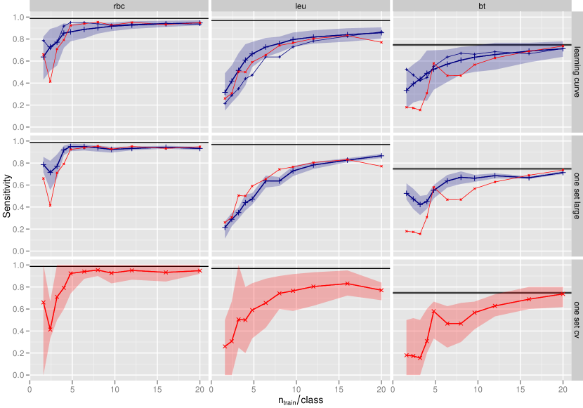
Figure 3: Learning curves of the real data set: sensitivities for recognition of red blood cells (rbc), leukocytes (leu), and BT-20 breast tumour cell line (bt). Black: Sensitivity observed for 100 iterations of 5-fold cross validation on the complete data set, approximating the best possible performance of a 10 latent variable PLS-LDA on this data set. Lines give the average, the shaded area covers the 5^th to 95^th percentile of iterations (bottom and middle row) and small data sets (top row). Thin lines: average “one set large” and “one set cv” (cross validation) performance are repeated in the rows above for easier comparison. Colours: blue performance measured with large test set, red performance measured by iterated cross validation. Bottom row: Learning curve of one growing data set, measured with 100$\times$ iterated 5-fold cross validation. Middle row: The same models as in the bottom row, but performance measured with large test set. The percentiles depict the instability of the surrogate models trained during iterated cross validation, but are subject only to low uncertainty due to the finite test sample size. Top row: sensitivity achieved for 100 different small data sets of size $n_{train}$, measured with the large test set.

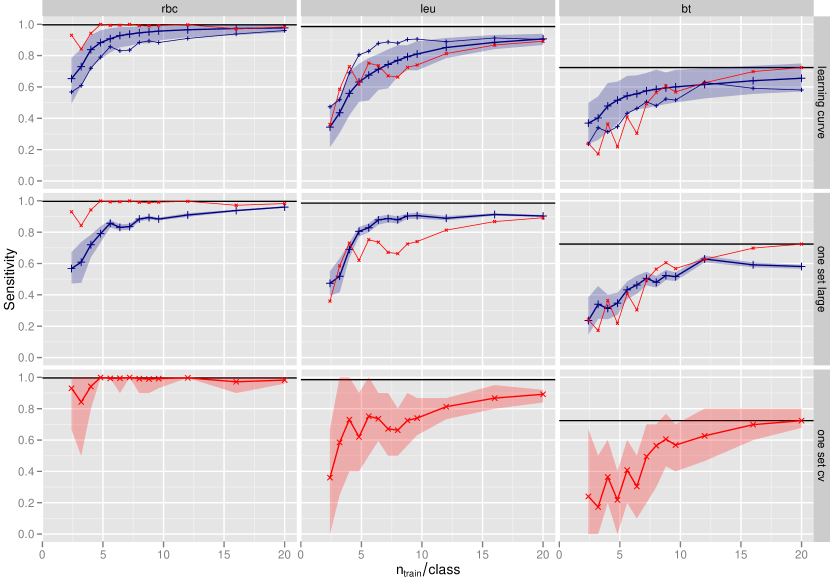
Figure 4: Learning curves of the simulated data set. This plot was generated analogously to fig 3. The only difference is that the best possible error (black lines) was measured with the large independent test set, see description of the data analysis.

The learning curve describes the performance of a given classifier for a problem as function of the training sample size [10]. The prediction errors a classifier makes may be divided into four categories:

1. the irreducible or Bayes error

2. the bias due to the model setup,

3. additional systematic deviations (bias), and

4. random deviations (variance)

The best possible performance that can be achieved with a given model setup consists of the Bayes error, i. e. the best possible performance for the best possible model, and the bias for $n_{train}\rightarrow\infty$. The latter two components depend on the training sample size, and tend to zero as more cases become available.

The general discussion of learning curves, e. g. [10, fig. 7.8], usually considers the combination of the first three error types (as function of the training sample size) which form the average (expected) performance of a given classification rule for a particular problem if $n_{train}$ training cases are available. The learning curve for a particular data set is known as conditional learning curve [10].

In the context of classification based on microarray data, both empirically fitted functions [1] and parametric methods based on the difference in gene expression [3, 4] have been used to estimate learning curves and necessary sample sizes for the training of well performing classifiers. An extension of Mukherjee et al. [1] has been applied to medical text classification [2].

Microarray (gene expression) data sets are similar to biospectroscopic data sets in their shape and size: in both cases the raw data typically consists of thousands of measurement channels (variates: genes, wavelengths) and typically hundreds to thousands of rows (expression profiles, spectra). However, they differ from typical biospectroscopic data sets in two important aspects. Firstly, biospectroscopic data sets often have rather large numbers of spectra of the same patient or batch while multiple measurements of the same subject are far less common in microarray studies. The data sets in Mukherjee et al. [1] have total patient numbers between 53 and 78 (plus one large set of 280 patients), these sample sizes unfortunately do not allow to check their extrapolated predictions of the performance. Secondly, the information with respect to the classification problem is usually spread out over wide spectral ranges in biospectroscopic classification. In contrast, microarray classification typically relies on rather few genes that carry information among a large number of noise-only variates [3, 4].

Figures 3 and 4 give the (unconditional) learning curves for the real and simulated data in the top rows (lines). With smaller sample sizes, the random uncertainty grows, and cannot be neglected: A particular data set of size $n_{train}$ may differ substantially from the average data set of size $n_{train}$. For each training sample size, 90 of the 100 small data sets had performance inside the shaded area.

For the simulated data, one such growing data set is shown exemplarily in the middle (true performance, i. e. tested with the large test set) and bottom rows (cross validation estimate of performance of the same model) of fig. 4. The example run performs exceptionally well for the leukocytes but roughly at the 5^th percentile with respect to all possible data sets of size $n_{train}$ of sensitivity for red blood cells and the BT-20 cell line. The example run of the real data (fig. 3) in general follows more closely the average sensitivity of data sets of the respective size. Learning curves reported for real data sets usually give one point measurement for each classifier set up and training sample size only and are usually calculated in the “retrospective” manner according to our definition above.

For the planning of necessary sample sizes needed to train good classifiers, both the expected performance in the top row of figs. 3 and 4 and the performance for a given growing data set as in the middle rows are of importance. The top rows answer the question how many samples should be collected if no samples are yet available for a specific problem, while the middle rows belong to the question how many more samples in addition to the already available ones should be collected.

In practice, however, neither the top nor the middle row learning curves are available, only (iterated) cross validation or out-of-bootstrap results are available from within a given data set. The results of the cross-validation in the bottom row are an unbiased estimate of the middle row (we use the actual training sample size of the surrogate models, i. e. $\frac{4}{5}$ of the sample size of the small data set). However, the cross validation is subject to much higher random uncertainty, as the total number of test cases is much lower than with the large test set used to calculate the middle rows.

As explained before, the random uncertainty comes from two sources: firstly, model instability, i. e. differences between surrogate models built with different training sets of the same size, and secondly testing uncertainty due to the finite number of spectra available for testing. The first is related to the number of training samples while the second depends on the number of test samples. Testing with the large test set reduces the second source of uncertainty but does not influence the variation due to model instability. The only difference between middle and bottom rows in figs. 3 and 4 are the test sets: exactly the same models are tested with the large test set (middle) and the spectra held out by the cross validation (bottom row). In other words, the bottom row is a “small test sample size” approximation to the middle row. The simulations use $n_{test}$ = 2 $\cdot$ 10⁴ for reference (top and middle row), meaning that the variation depicted in middle row of fig. 4 is caused only by model instability. On contrast, for the real data, only ca. 350 – 540 reference test spectra are available and uncertainty due to the finite test sample size can contribute substantially to the observed variation in the middle row of fig. 3. However, the total random uncertainty on the iterated cross validation is dominated by the huge random uncertainty due to testing only with the up to 25 samples of the small data set.

This uncertainty is large enough to mask important features of the learning curve of the growing data set: in our example run for the simulated data, the sensitivity for erythrocytes is largely overestimated (other runs show equally large underestimation). The exceptionally good performance for the leukocytes with 4 – 10 training samples is not only not detected by the cross validation but in fact two dips appear in the cross validation estimate of the example data set’s learning curve. For the BT-20 cell line, we observe an oscillating behaviour with the addition of single cases up to a data set size of 9 samples (i. e. on average 7.2 training samples). Of course, we observe also runs that match the true (reference) learning curve of the particular data set more closely. But even then the percentiles indicate that the results are not reliable estimates of the learning curve of that data set.

The cross validation of the real data set underestimates the sensitivity for red blood cells for the extremely small sample sizes, however the general development of sensitivity as function of the training sample size of the example run is correctly reproduced. Also the learning curve for the leukocytes is quite closely matched. For the BT-20 cells, however, the cross validation again does not even resemble the shape of the example data set’s learning curve.

In conclusion, the average performances observed during the iterated cross validation do not reliably recover the correct shape of the learning curve of the particular data set for our small sample size scenarios (middle rows), much less that of the performance of any data set of the respective training sample size (top rows). In contrast, the actual performance of the classifiers (top and middle rows) is acceptable to very good considering the actual training sample sizes: with 20 training cases per class, red blood cells are almost perfectly recognized, sensitivities around 0.90 are achieved for leukocytes and even about 2 out of 3 of the very difficult BT-20 breast cancer cells are recognized correctly.

4 Sample Size Requirements for Classifier Testing

Thus, the precise measurement of the classifier performance turns out to be more complicated in such small sample size situations. Sample size planning for classification therefore needs to take into account also the sample size requirements for the testing of the classifier. We will discuss here two important scenarios that allow estimating required test sample sizes: firstly, specifying an acceptable width for a confidence interval of the performance measure and secondly the number of test cases needed for a comparison of classifiers.

4.1 Specifying Acceptable Confidence Interval Widths

## Loading required package: ggplot2

For Bernoulli processes, several approaches exist to estimate confidence intervals for the true probability $p$ given the observed probability $\hat{p}$ and the number of tests $n$, see [23, 24] for recommendations particularly in small sample size situations. For the following discussion, we use the Bayes method with a uniform prior to obtain the minimal-length or highest posterior density (HPD) interval [25, 26]. For details about the statistical properties of this method, please refer to [24]. Package binom[25] offers a variety of other methods that can easily be used by the interested reader instead.

From a computational point of view, this method is convenient as the calculations can be formulated using the Beta-distribution which allows to compute results not only for discrete numbers of events $k$, but for real $k$. Thus, $\hat{p}$ obtained from testing many spectra can be used with a test sample size $n_{test}$ equalling e. g. the number of test patients or batches.

Confidence intervals for the true proportion are calculated as function of the number of test samples (denominator of the proportion) and the observed proportion $\hat{p}$. The intervals are widest for $\hat{p}=0.5$ and narrowest for $\hat{p}=0$ or $1$. Consequently, the necessary test sample size to measure the performance with a pre-specified precision can be calculated, either in a conservative (worst-case) fashion for $\hat{p}=0.5$ or using existing knowledge/expectations about the achievable performance.

Figure 5 shows the 95 % confidence intervals for different observed performances as function of the test sample size. For our example application, e. g. the sensitivity of the leukocyte class reaches 0.90 rather quickly. If that model were tested with 100 leukocytes (i. e. four times as many as in our largest small data sets) and 90 of them were correctly recognized, the 95 % confidence interval would range from 0.83 (which would be considered quite bad as leukocytes are fairly easy to recognize) to 0.94 – which in the context of our classification task would be translated to “quite good”. In other words, the confidence interval would still be too wide to allow a practical judgment of the classifier.

Similarly, already with 4 – 5 training spectra (out of 6 total red blood cell spectra in the data set), we observed perfect recognition of red blood cells in the simulation example’s cross validation. But the 95 % confidence interval still reaches down to 0.65. However, for $\hat{p}=1$ the confidence intervals narrow very soon, and “already” with 58 test samples the lower limit of the 95 % confidence interval reaches 0.95 (see fig. 6).

Figure 6 gives the width of the Bayesian confidence interval as function of the test sample size for different observed values of the performance. Note that specifying confidence interval widths to be less than 0.10 with expected observed performance between 0.90 and 0.95 already corresponds to requiring between 3 – 5$\frac{1}{2}$ times as many test samples as we consider typically available in biospectroscopy. For confidence interval widths of less than 0.05 which would allow to distinguish the practical categories “bad” and “very good”, hundreds of test cases are required. Also, this estimation of required sample sizes is very sensitive to the true proportion $p$: if $p$ were in fact only 0.89 instead of the 0.9 assumed in the example, 153 instead of 141 test samples would be required to reach the specified confidence interval width.

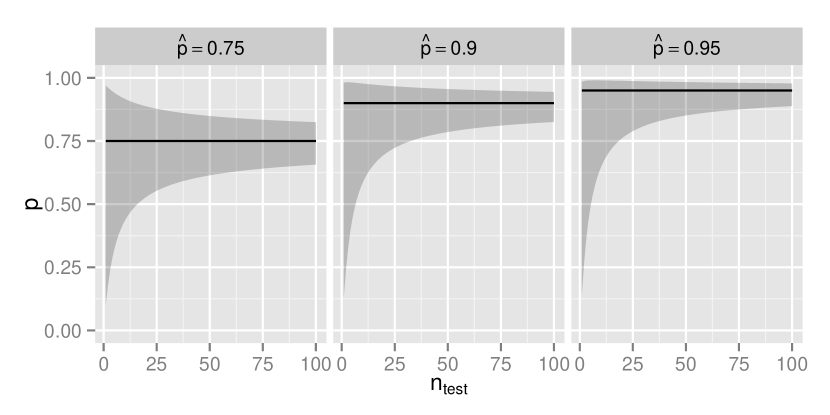
Figure 5: 95 % confidence intervals for different observed performances $\hat{p}$ as function of $n_{test}$. If 90 out of 100 samples of a class are recognized correctly (e. g. sensitivity of the leukocytes with 25 training samples), the 95 % confidence interval for the sensitivity ranges from 0.83 to 0.94 – which in the context of our classification task reads as being between “quite bad” and “really good”.

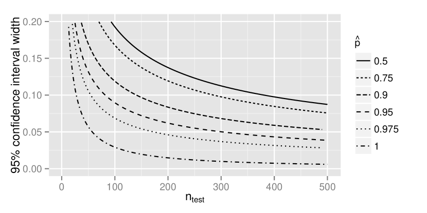
Figure 6: 95 % confidence interval widths for different observed performances $\hat{p}$ as function of $n_{test}$. $\hat{p}=0.5$ and $1$ give the widest and narrowest possible confidence interval widths. E. g. If the confidence interval should not be more than 0.1 wide while a sensitivity of 0.9 is expected, $n_{test}\geq 141$ samples need to be tested.

4.2 Demonstrating that a New Classifier is Better

A second important scenario that allows to specify necessary test sample sizes is demonstrating superiority to an already known classifier. E. g., the instrument is improved and the resulting advantage should be demonstrated. A rough estimate of the performance of the new instrument is available. How many samples are needed in order to prove the superiority of the new approach?

From a statistics point of view, comparing classifier performance is a typical hypothesis testing task. R package Hmisc [27] provides functions for power (bpower) and sample size estimation (bsamsize) of independent proportions with unequal test sample sizes as described by Fleiss et al. [28]. The approximation overestimates power for small sample sizes [29]. However, this is not of much consequence here, as the calculated sample sizes will anyways be rough guesstimates rather than exact numbers of required samples: Firstly, the exact performance of the improved classifier is unknown, so the sample size planning needs to check the sensitivity of the calculated numbers to this assumption. Secondly, the actual power of the calculated scenario can be checked by bpower.sim.

Assume our recognition of BT-20 cells were improved from the 0.75 sensitivity we obtain with 20 training samples / class to 0.90. A quick estimate of the necessary test sample size reveals that in this scenario, the maximal obtainable power (setting $n_{test}$ for the new model to 10⁵ as infinite for practical purposes) is $1-\beta=$ 0.62. In other words, there is no chance to prove the superiority of the new classifier with anything close to an acceptable type II error due to the small test sample size available for the old model. The comparisons have most power if the tests are performed with equal sample sizes. For this case, tables are also available in Fleiss and Paik [30]. In our example, the usual power of 0.8 (i. e. type II error $\beta=0.2$; with type I error$\alpha=0.05$) needs at least 100 independent test cases truly belonging to class bt for each of the models. Note that paired tests can be much more powerful, thus requiring less samples. Paired tests can be used when the same cases can be measured again (impossible for our study: new cell culture batches need to be grown) or if the improvement is in the data analysis and therefore the same instrumental data can be analysed by both methods.

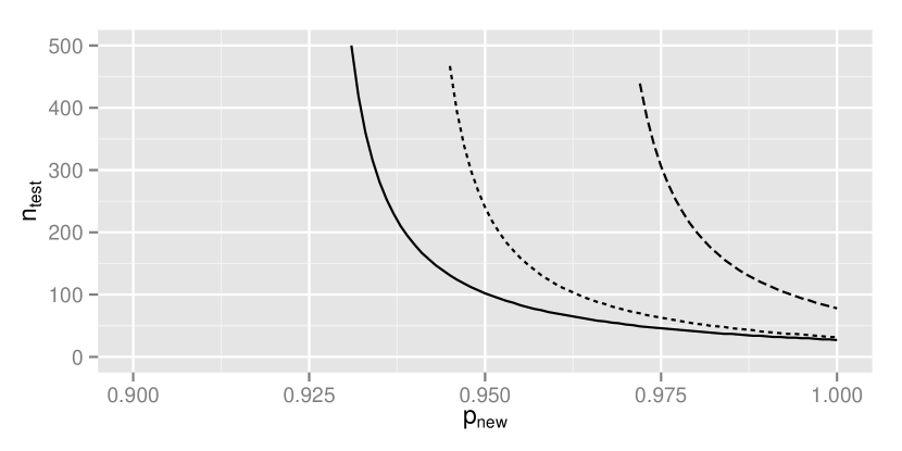
Figure 7: Test sample size necessary to demonstrate superiority of an improved model of sensitivity $p_{new}$, assuming the “old” model had $p_{old}$ = 0.75 sensitivity and was tested with $n_{test}$ = 25 samples and accepting a type I error of $\alpha=0.05$ and a type II error $\beta=0.2$ (solid line). Dotted: test sample size for the second model with $\alpha=\beta=0.10$. However, if $\alpha=\beta=0.05$ is required (dashed), even a model with 0.975 true sensitivity needs to be tested with at least 300 cases and 116 cases are necessary to demonstrate the superiority of an improved model truly achieving 0.99 sensitivity.

If we could achieve 0.975 sensitivity for BT-20 cells, we would need to test with 63 test cases (accepting $\alpha=\beta=0.10$). Figure 7 shows that this is very sensitive to the assumed quality of the new model: if the new model has in fact “only” a sensitivity of 0.96 (corresponding to ca. 1 additional misclassification out of 63 test cases), already 117 or almost twice as many test cases are needed. Note that this is a rather extreme example as it means one order of magnitude (0.25 to 0.025) reduction in the fraction of unrecognized BT-20 cells, which is much larger than the improvements considered in the practice of biospectroscopic classification.

In conclusion, well working classifiers need to be validated with at least 75 test cases in order to obtain confidence intervals that are narrow enough to draw practical conclusions about the model. Demonstrating superiority of a new, improved classifier in general needs even more test cases and often will be impossible at all if the test sample size for the old classifier was small.

5 Summary

Using a Raman spectroscopic five class classification problem as well as simulated data based on the real data set, we compared the sample sizes needed to train good classifiers with sample sizes needed to demonstrate that the obtained classifiers work well. Due to the smaller test sample size, sensitivities are more difficult to determine precisely than specificities or overall hit rates.

Using typical small sample sizes of up to 25 samples per class, we calculated learning curves (sensitivity as function of the training sample size) using 100$\times$ iterated $5$-fold cross validation. While the general shape of the learning curve could be determined correctly for the very easily recognized red blood cells, for more difficult recognition tasks not even the correct shape of the learning curve can be determined reliably within the small data set as the precise measurement of classifier performance requires rather large test sample sizes (> 75 cases).

In consequence, we calculate necessary test sample sizes for different pre-specified testing scenarios, namely specifying acceptable widths for the confidence interval of the true sensitivity and the number of test samples needed to demonstrate superiority of one classifier over another. In order to obtain confidence interval widths $\leq$ 0.1, 140 test samples are necessary when 90 % sensitivity is expected. In contrast, the recognition of leukocytes in our example application reaches 90 % sensitivity already with about 20 training samples. Comparison of classifiers was found to require even larger test sample sizes (hundreds of statistically independent cases) in the general case.

In conclusion, we recommend to start sample size planning for classification by specifying acceptable confidence interval widths for the expected sensitivities. This will lead to sample sizes that allow retrospective calculation of learning curves and a refined sample size planning in terms of both test and training sample size can then be done.

Supplementary file I: Confusion matrices for table 1

We give here the complete confusion tables for the models described in table 1. The counts are divided by the number of test samples truly belonging to the respective class and averaged over all runs, i. e. the diagonal elements are the sensitivities, the other entries are the specificities with respect to that particular misclassification.

Bayes Performance for Simulated Data LDA Model

conf.mat.bayes

##      pred
## ref   rbc leu  mcf   bt  oci
##   rbc   1   0 0.00 0.00 0.00
##   leu   0   1 0.00 0.00 0.00
##   mcf   0   0 0.95 0.03 0.02
##   bt    0   0 0.04 0.91 0.05
##   oci   0   0 0.02 0.03 0.94

n

##   rbc   leu   mcf    bt   oci
## 40000 40000 40000 40000 40000

Bayes Performance for Simulated Data 10 latent variable PLS-LDA

conf.mat.plsbayes

##      pred
## ref   rbc  leu  mcf   bt  oci
##   rbc   1 0.00 0.00 0.00 0.00
##   leu   0 0.99 0.01 0.00 0.01
##   mcf   0 0.00 0.87 0.06 0.07
##   bt    0 0.00 0.14 0.72 0.13
##   oci   0 0.00 0.04 0.09 0.86

n

##   rbc   leu   mcf    bt   oci
## 40000 40000 40000 40000 40000

Average “Bayes” Performance for Real Data as used in the paper

confmat.bayes

##      pred
## ref    rbc  leu  mcf   bt  oci
##   rbc 0.99 0.01 0.00 0.00 0.00
##   leu 0.00 0.97 0.01 0.00 0.02
##   mcf 0.00 0.00 0.91 0.04 0.05
##   bt  0.00 0.00 0.13 0.75 0.13
##   oci 0.00 0.01 0.04 0.07 0.89

n

## rbc leu mcf  bt oci
## 372 569 558 532 518

Average “Bayes” Performance for Real Data batch-wise validation

confmat.batch

##      pred
## ref    rbc  leu  mcf   bt  oci
##   rbc 0.98 0.02 0.00 0.00 0.00
##   leu 0.00 0.87 0.03 0.04 0.06
##   mcf 0.00 0.00 0.33 0.37 0.30
##   bt  0.00 0.00 0.32 0.38 0.30
##   oci 0.00 0.02 0.31 0.36 0.31

n

## rbc leu mcf  bt oci
## 372 569 558 532 518

This file is supplementary material for: C. Beleites, U. Neugebauer, T. Bocklitz, C. Krafft and J. Popp: Sample size planning for classification models. Analytica Chimica Acta, 2013, 760 (Special Issue: Chemometrics in Analytical Chemistry 2012), 25–33, DOI: 10.1016/j.aca.2012.11.007.

Supplementary file II: R code for section 4

Specifying Acceptable Confidence Interval Widths

Calculation of the Bayesian confidence intervals and their widths

require("binom")
require("ggplot2")

We consider test sample sizes up to 500:

n <- 1:500

Now calculate confidence intervals for different observed performance values $\hat{p}$ between 0.5 and 1. As binom.bayes does not converge for all combinations of $n$ and $\hat{p}$, keep only results where the actual confidence level is 0.95 $\pm 10^{-4}$ (a bunch of warnings will be thrown; filter the results without adequate coverage afterwards). The uniform prior is selected by setting both prior.shape1 and prior.shape2 to 1.

confint <- lapply(c(0.5, 0.75, 0.9, 0.95, 0.975, 1), function(p) {
    tmp <- binom.bayes(n = n, x = p * n, prior.shape1 = 1, prior.shape2 = 1)
    tmp$phat <- p
    subset(tmp, sig >= 0.05 - 1e-04 & sig <= 0.05 + 1e-04)
})
confint <- do.call(rbind, confint)

Add column containing the width of the confidence interval:

confint$width <- confint$upper - confint$lower

head(confint)

##   method   x n shape1 shape2 mean   lower  upper  sig phat  width
## 1  bayes 0.5 1    1.5    1.5  0.5 0.06083 0.9392 0.05  0.5 0.8783
## 2  bayes 1.0 2    2.0    2.0  0.5 0.09430 0.9057 0.05  0.5 0.8114
## 3  bayes 1.5 3    2.5    2.5  0.5 0.12275 0.8772 0.05  0.5 0.7545
## 4  bayes 2.0 4    3.0    3.0  0.5 0.14663 0.8534 0.05  0.5 0.7067
## 5  bayes 2.5 5    3.5    3.5  0.5 0.16681 0.8332 0.05  0.5 0.6664
## 6  bayes 3.0 6    4.0    4.0  0.5 0.18405 0.8159 0.05  0.5 0.6319

Sample sizes used in the text:

(nleuko <- min(subset(confint, phat == 0.9 & width <= 0.1)$n))

## [1] 141

(nery <- min(subset(confint, phat == 1 & width <= 0.05)$n))

## [1] 58

tmp <- binom.bayes(n = n, x = 0.89 * n, prior.shape1 = 1, prior.shape2 = 1)
tmp$width <- tmp$upper - tmp$lower
(nleuko89 <- min(subset(tmp, width <= 0.1)$n))

## [1] 153

95 % confidence interval for 90 correct out of 100 tested leukocytes:

binom.bayes(n = 100, x = 90, prior.shape1 = 1, prior.shape2 = 1)

##   method  x   n shape1 shape2   mean  lower  upper  sig
## 1  bayes 90 100     91     11 0.8922 0.8254 0.9444 0.05

95 % confidence interval for 6 correct out of 6 tested erythrocytes:

binom.bayes(n = 6, x = 6, prior.shape1 = 1, prior.shape2 = 1)

##   method x n shape1 shape2  mean  lower upper  sig
## 1  bayes 6 6      7      1 0.875 0.6518     1 0.05

Generate the plots:

ggplot (subset (confint, phat %in% c (.75, .9, .95) & n <= 100)) +
  geom_ribbon (aes (x = n, ymin = lower, ymax = upper), alpha = 0.25) +
  facet_grid (. ~ phat, labeller = label_bquote(expr = hat (p) == .(x))) +
  geom_line (aes (x = n, y = phat)) +
  ylab ("p") + xlab (expression (n [test]))

ggplot (subset (confint, width <= 0.2)) +
  geom_line (aes (x = n, y = width, lty = as.factor (phat))) +
  scale_linetype_discrete (expression (hat (p))) +
  ylim (0, .2) + ylab ("95% confidence interval width") +
  xlab (expression (n [test]))

Demonstrating that a New Classifier is Better

require("Hmisc")

Assume our recognition of BT-20 cells were improved from the 75 % sensitivity we obtain with 20 training samples / class to 90 % (Bayes error for LDA of the simulated data). A quick estimate of the necessary test sample size reveals that in this scenario, the maximal obtainable power (setting $n_{test}$ for the new model to 10⁵ as infinite for practical purposes) is $1-\beta=$

bpower.sim(p1 = 0.75, p2 = 0.9, n1 = 25, n2 = 1e+05, nsim = 1e+05)

##  Power  Lower  Upper
## 0.6218 0.6188 0.6248

Required sample size for equal test sample sizes for both classifiers:

bsamsize(p1 = 0.75, p2 = 0.9)

##    n1    n2
## 99.54 99.54

Prepare necessary sample size if old classifier was tested with 25 samples. bsamsize only accepts fractions of samples, not directly specifying $n_{1}$ = $n_{old}$. Thus, we need to find the fraction that corresponds to $n_{old}$ = 25 and from there calculate $n_{new}$.

target.fun <- function(fraction, ..., n.old) {
    n1 <- bsamsize(fraction = fraction, ...)[1]
    (n1 - n.old)^2
}

est.n2 <- function(p2, ..., n.old) {
    fraction <- optimize(target.fun, lower = 1e-05, upper = 0.5, ..., p2 = p2,
        n.old = n.old)$minimum
    ceiling(n.old/fraction - n.old)
}

We consider $p_{1}=0.75,p_{2}\in[0.9,1]$ and $n_{old}=25$ (target value for $n_{1}$) for the three different type I and type II errors discussed in the text:

p2 <- seq(0.9, 1, by = 0.001)

n2 <- sapply(p2, est.n2, power = 0.95, p1 = 0.75, n.old = 25)
df <- data.frame(p2 = p2, n2 = n2, power = 0.95)

n2 <- sapply(p2, est.n2, power = 0.9, alpha = 0.1, p1 = 0.75, n.old = 25)
df <- rbind(df, data.frame(p2 = p2, n2 = n2, power = 0.9))

n2 <- sapply(p2, est.n2, power = 0.8, p1 = 0.75, n.old = 25)
df <- rbind(df, data.frame(p2 = p2, n2 = n2, power = 0.8))

ggplot (data = subset (df, n2 <= 500), aes (x = p2, y = n2, lty = as.factor (power))) +
  geom_line () + ylim (0, 500) + xlim (0.90, 1) +
  xlab (expression (p [new])) + ylab (expression (n[test,~new]))

The example values are extracted from the data.frame in the paper:

subset(df, p2 == 0.975 & power == 0.9, n2)

##     n2
## 177 63

subset(df, p2 == 0.96 & power == 0.9, n2)

##      n2
## 162 117

but can also be calculated directly with the functions defined above:

est.n2(p1 = 0.75, p2 = 0.975, power = 0.9, alpha = 0.1, n.old = 25)

## [1] 63

est.n2(p1 = 0.75, p2 = 0.96, power = 0.9, alpha = 0.1, n.old = 25)

## [1] 117

Information on Using and Compiling this file

This document is provided in two forms. The .Rnw is a knitr (Sweave) file. It can be processed in R using:

require("knitr")
knit("supplementary-code.Rnw")

which produces a LaTeX document that can be compiled into the .pdf by pdflatex (uncomment the document header and footer as indicated).

License

You may use this document under the Creative Commons CC BY-SA License version 3.0 (see http://creativecommons.org/licenses/by-sa/3.0/)

As attribution, please cite: C. Beleites, U. Neugebauer, T. Bocklitz, C. Krafft and J. Popp: Sample size planning for classification models. Analytica Chimica Acta, 2013, 760 (Special Issue: Chemometrics in Analytical Chemistry 2012), 25–33, DOI: 10.1016/j.aca.2012.11.007.

R Session Information

sessionInfo()

## R version 2.15.2 (2012-10-26)
## Platform: x86_64-pc-linux-gnu (64-bit)
##
## locale:
##  [1] LC_CTYPE=de_DE.UTF-8       LC_NUMERIC=C
##  [3] LC_TIME=de_DE.UTF-8        LC_COLLATE=de_DE.UTF-8
##  [5] LC_MONETARY=de_DE.UTF-8    LC_MESSAGES=de_DE.UTF-8
##  [7] LC_PAPER=C                 LC_NAME=C
##  [9] LC_ADDRESS=C               LC_TELEPHONE=C
## [11] LC_MEASUREMENT=de_DE.UTF-8 LC_IDENTIFICATION=C
##
## attached base packages:
## [1] splines   stats     graphics  grDevices utils     datasets  methods
## [8] base
##
## other attached packages:
## [1] Hmisc_3.10-1     survival_2.36-14 ggplot2_0.9.2.1  binom_1.0-5
## [5] lattice_0.20-10  knitr_0.8
##
## loaded via a namespace (and not attached):
##  [1] cluster_1.14.3     colorspace_1.2-0   dichromat_1.2-4
##  [4] digest_0.5.2       evaluate_0.4.2     formatR_0.6
##  [7] grid_2.15.2        gtable_0.1.2       labeling_0.1
## [10] MASS_7.3-22        memoise_0.1        munsell_0.4
## [13] plyr_1.7.1         proto_0.3-9.2      RColorBrewer_1.0-5
## [16] reshape2_1.2.1     scales_0.2.1       stringr_0.6.1
## [19] tools_2.15.2

References

- [1] S. Mukherjee, P. Tamayo, S. Rogers, R. Rifkin, A. Engle, C. Campbell, T. R. Golub, J. P. Mesirov, Estimating dataset size requirements for classifying DNA microarray data., J Comput Biol 10 (2) (2003) 119–142. doi:10.1089/106652703321825928.
- [2] R. L. Figueroa, Q. Zeng-Treitler, S. Kandula, L. H. Ngo, Predicting sample size required for classification performance., BMC Med Inform Decis Mak 12 (1) (2012) 8. doi:10.1186/1472-6947-12-8.
- [3] K. K. Dobbin, R. M. Simon, Sample size planning for developing classifiers using high-dimensional DNA microarray data., Biostatistics 8 (1) (2007) 101–117. doi:10.1093/biostatistics/kxj036.
- [4] K. K. Dobbin, Y. Zhao, R. M. Simon, How large a training set is needed to develop a classifier for microarray data?, Clin Cancer Res 14 (1) (2008) 108–114. doi:10.1158/1078-0432.CCR-07-0443.
- [5] A. Jain, B. Chandrasekaran, Dimensionality and Sample Size Considerations in Pattern Recognition Practice, in: P. R. Krishnaiah, L. Kanal (Eds.), Handbook of Statistics, Vol. II of Handbook of Statistics, North-Holland, Amsterdam, 1982, Ch. 39, pp. 835 – 855.
- [6] S. Raudys, A. Jain, Small Sample Size Effects in Statistical Pattern Recognition: Recommendations for Practitioners, IEEE Transactions on Pattern Analysis and Machine Intelligence 13 (1991) 252–264. doi:http://doi.ieeecomputersociety.org/10.1109/34.75512.
- [7] H. M. Kalayeh, D. A. Landgrebe, Predicting the required number of training samples., IEEE Trans Pattern Anal Mach Intell 5 (6) (1983) 664–667.
- [8] U. Neugebauer, T. Bocklitz, J. H. Clement, C. Krafft, J. Popp, Towards detection and identification of circulating tumour cells using Raman spectroscopy., Analyst 135 (12) (2010) 3178–3182. doi:10.1039/c0an00608d.
- [9] U. Neugebauer, J. H. Clement, T. Bocklitz, C. Krafft, J. Popp, Identification and differentiation of single cells from peripheral blood by Raman spectroscopic imaging., J Biophotonics 3 (8-9) (2010) 579–587. doi:10.1002/jbio.201000020.
- [10] T. Hastie, R. Tibshirani, J. Friedman, The Elements of Statistical Learning; Data mining, Inference andPrediction, 2nd Edition, Springer Verlag, New York, 2009.
- [11] E. R. Dougherty, C. Sima, J. Hua, B. Hanczar, U. M. Braga-Neto, Performance of Error Estimators for Classification, Current Bioinformatics 5 (2010) 53–67.
- [12] R. Kohavi, A Study of Cross-Validation and Bootstrap for Accuracy Estimation and Model Selection, in: C. S. Mellish (Ed.), Artificial Intelligence Proceedings 14th International Joint Conference, 20 – 25. August 1995, Montréal, Québec, Canada, Morgan Kaufmann, USA, 1995, pp. 1137 – 1145.
- [13] C. Beleites, R. Baumgartner, C. Bowman, R. Somorjai, G. Steiner, R. Salzer, M. G. Sowa, Variance reduction in estimating classification error using sparse datasets, Chem.Intell.Lab.Syst. 79 (2005) 91 – 100.
- [14] K. H. Esbensen, P. Geladi, Principles of Proper Validation: use and abuse of re-sampling for validation, J. Chemometrics 24 (3-4) (2010) 168–187.
- [15] R Development Core Team, R: A Language and Environment for Statistical Computing, R Foundation for Statistical Computing, Vienna, Austria, ISBN 3-900051-07-0 (2011).
- [16] C. Beleites, V. Sergo, hyperSpec: a package to handle hyperspectral data sets in R, R package v. 0.98-20120725 (2012).
- [17] A. Genz, F. Bretz, T. Miwa, X. Mi, F. Leisch, F. Scheipl, T. Hothorn, mvtnorm: Multivariate Normal and t Distributions, R package v. 0.9-9992 (2012).
- [18] A. Genz, F. Bretz, Computation of Multivariate Normal and t Probabilities, Lecture Notes in Statistics, Springer-Verlag, Heidelberg, 2009.
- [19] C. Beleites, cbmodels: Collection of "combined" models: PCA-LDA, PLS-LDA, etc., R package v. 0.5-20120731 (2012).
- [20] R. Wehrens, B.-H. Mevik, pls: Partial Least Squares Regression (PLSR) and Principal Component Regression (PCR), R package version 2.1-0 (2007).
- [21] W. N. Venables, B. D. Ripley, Modern Applied Statistics with S, 4th Edition, Springer, New York, 2002, ISBN 0-387-95457-0.
- [22] M. Barker, W. Rayens, Partial least squares for discrimination, Journal of Chemometrics 17 (3) (2003) 166–173.
- [23] L. Brown, T. Cai, A. DasGupta, Interval Estimation for a Binomial Proportion, Statistical Science 16 (2001) 101–133.
- [24] A. M. Pires, C. Amado, Interval Estimators for a Binomial Proportion: Comparison of Twenty Methods, Revstat – Statistical Journal 6 (2) (2008) 165–197.
- [25] S. Dorai-Raj, binom: Binomial Confidence Intervals For Several Parameterizations, R package version 1.0-5 (2009).
- [26] E. Jaynes, Probability theory : the logic of science, Cambridge University Press, Cambridge, UK New York, NY, 2003.
- [27] F. E. Harrell Jr with contributions from many other users., Hmisc: Harrell Miscellaneous, R package v. 3.9-3 (2012).
- [28] J. L. Fleiss, A. Tytun, H. K. Ury, A Simple Approximation for Calculating Sample Sizes for Comparing Independent Proportions, Biometrics 36 (2) (1980) 343–346. doi:10.2307/2529990.
- [29] M. Vorburger, B. Munoz, Simple Power Calculations: How Do We Know We Are Doing Them the Right Way?, in: Proceedings of the Survey Research Methods Section, American Statistical Association, 2006, pp. 3809–3812.
- [30] B. L. Joseph L. Fleiss, M. C. Paik, Statistical Methods for Rates and Proportions, 3rd Edition, Wiley-Interscience, New Jersey, 2003.
- [31] H. Wickham, ggplot2: elegant graphics for data analysis, Springer New York, 2009.