Study of planar Ising ferromagnet on the triangular lattice with selective dilution

Abstract

In the paper the Curie temperatures of selectively diluted planar Ising ferromagnet on the triangular lattice are calculated vs. concentration of magnetic atoms. Various analytical approaches are compared with the exact numerical calculations for finite clusters, as well as with the exact analytical solutions for the triangular and honeycomb lattices.

I Introduction

The studies of low-dimensional magnets have presented a topical item for many years. The investigations include both 1D and 2D magnets, as well as bilayers, thin films and multilayers. Many different theoretical methods have been employed; in some cases [1–6] the exact solutions are available.

As far as approximate methods are concerned, one should mention the Green Function (GF) [7–9] and spectral density [10] methods, Renormalization Group (RG) approach [11, 12], including Mean-Field Renormalization Group (MFRG) [13, 14] and Effective-Field Renormalization Group (EFRG) [15], Spin-Wave (SW) techniques [16–18], High Temperature Series Expansion (HTSE) [19] and Monte Carlo (MC) simulations [20, 21]. Many other approaches like Coherent Anomaly Method (CAM) together with transfer matrix technique [22] and Effective Field Methods (EFM) with correlations [23] should also be mentioned. Recently, Cluster Variational Method in the Pair Approximation (PA) has been adopted for studies of the bilayer [24] and bi-multilayer [25] systems.

The aim of the present paper is to study the ferromagnetic Ising model with spin $S=1/2$ on the Planar Triangular (PT) lattice with selective dilution. By the selective dilution we mean the dilution of only one sublattice, whereas the PT magnet can be, in general, decomposed into three interpenetrating sublattices. Regarding antiferromagnetism and the problem of frustration, such selectively diluted model has been considered by Kaya and Berker [26]. To the best of our knowledge, as far as ferromagnetism is concerned, the model has not been studied yet.

The model is interesting from the theoretical point of view, for by changing the selective dilution parameter we are able to pass continuously from the ideal PT lattice (without dilution) to the honeycomb lattice, where one sublattice is completely empty. On the other hand, for those two cases the exact solutions for the Curie temperatures do exist [2]. In this paper we will concentrate on the Curie temperature calculations for arbitrary concentration of magnetic atoms in the selectively diluted sublattice. Thus, we consider an intermediate situation between those two limiting cases, which were examined exactly by Wannier [2].

In the next Section, the outline of the theoretical methods will be given, and the respective formulas for the phase transition temperatures will be presented. With the help of numerical calculations we are able to compare the results of several theoretical approaches, namely the Molecular Field Approximation (MFA), Effective Field Theory (EFT), Pair Approximation (PA) method, as well as the Exact Calculation for Finite Clusters (ECFC). The results will be presented in the plots and discussed.

II Theoretical methods

Let us consider the ferromagnetic Ising model with spin $S=1/2$ on the PT lattice with selective dilution. The diluted lattice is illustrated in Fig. 1. Following Kaya and Berker [26] we keep decomposition of the PT lattice into three interpenetrating sublattices $a$, $b$ and $c$, of which, for the ferromagnetic case the sublattices $a$ and $b$ will be equivalent. The sublattice $c$ is distinguished in the system by the random dilution of the spins. If we denote by $p$ the concentration of spins on $c$-sublattice, the case of $p=0$ corresponds to the honeycomb lattice, whereas $p=1$ stands for the non-diluted triangular lattice.

The Hamiltonian of the system is in the form of:

$${\cal H}=-J\sum\limits_{\left(i_{a},j_{b}\right)}S_{i_{a}}^{z}S_{j_{b}}^{z}-J\sum\limits_{\left(i_{a},j_{c}\right)}S_{i_{a}}^{z}S_{j_{c}}^{z}\xi_{j_{c}}-J\sum\limits_{\left(i_{b},j_{c}\right)}S_{i_{b}}^{z}S_{j_{c}}^{z}\xi_{j_{c}}$$ (1)

where $J>0$ is the exchange interaction coupling, and $\left(i_{\alpha},j_{\beta}\right)$ means the summation extending over nearest neighbour pairs of spins from sublattice $\alpha$ and $\beta$. $\xi_{j_{c}}$ are quenched, uncorrelated random variables chosen to be equal 1 with probability $p$ when the site $j_{c}$ is ocupied by a magnetic atom and 0 with probability $1-p$ otherwise.

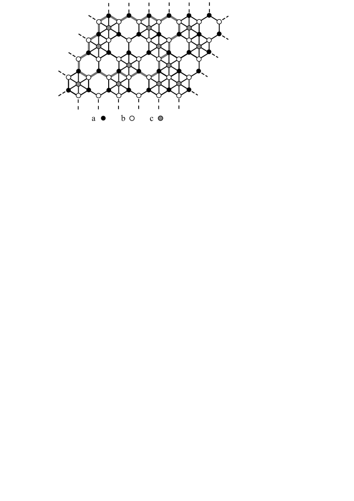
Figure 1: The triangular lattice divided into three interpenetrating sublattices: $a$, $b$ and $c$. The sublattice $c$ is randomly diluted. The thick grey line surrounds a cluster containing $3\times 4$ hexagons, used for exact calculations.

II.1 Molecular Field Approximation (MFA)

In this simplest approach the sublattice magnetizations $m_{a}=\left<S_{i_{a}}^{z}\right>$, $m_{b}=\left<S_{i_{b}}^{z}\right>$ and $m_{c}=\left<S_{i_{c}}^{z}\right>$ are described by three coupled MFA equations. In the vicinity of the Curie temperature the equations can be linearized and presented as follows:

$$m_{a} = \frac{3}{4}\beta_{\rm C}J\left(m_{b}+m_{c}\,p\right)$$

$$m_{b} = \frac{3}{4}\beta_{\rm C}J\left(m_{a}+m_{c}\,p\right)$$

$$m_{c} = \frac{3}{4}\beta_{\rm C}J\left(m_{a}+m_{b}\right)$$ (2)

where $\beta_{\rm C}=1/k_{\rm B}T_{\rm C}$, and $T_{\rm C}$ denotes the Curie temperature.

It is convenient to introduce the variable $t_{\rm C}=k_{\rm B}T_{\rm C}/J$ which is a dimensionless Curie temperature. Then, assuming symmetry condition for the ferromagnet $m_{a}=m_{b}\neq m_{c}$, and demanding that the determinant of eqs. (2) must be zero, we obtain the equation for the Curie temperature in MFA:

$$8t_{\rm C}^{2}-6t_{\rm C}-9p=0.$$ (3)

The physical solution is then of the form:

$$t_{\rm C}=\frac{3}{8}\left(1+\sqrt{1+8p}\right)$$ (4)

and is straightforward for numerical calculation.

II.2 Effective Field Theory (EFT)

By the EFT we mean the method proposed by Honmura and Kaneyoshi [27], which takes into account autocorrelations but neglects the spin-pair correlations. Among its many applications, the method has recently been applied for the triangular lattice with uniform dilution [28]. It is based on the exact Callen-Suzuki identity of the form:

$$\left<S_{i_{\alpha}}^{z}\right>=\frac{1}{2}\left<\tanh\frac{1}{2k_{\rm B}T}\left(J\sum_{j_{\beta}\in i_{\alpha}}S_{j_{\beta}}^{z}\xi_{j_{\beta}}\right)\right>.$$ (5)

where $\xi_{j_{\beta}}=1$, if $\beta=a,b$ and $j_{\beta}\in i_{\alpha}$ denotes a lattice site being nearest neighbour of the site $i_{\alpha}$ .

Applying the differential operator method [27], together with the decoupling procedure for the mean value of multi-spin products, the local magnetizations can be calculated. The coupled equations for the sublattice magnetizations have polynomial form and can be linearized near the continuous phase transition points. For the system in question, with the general sublattice magnetizations $m_{a}$, $m_{b}$ and $m_{c}$, the Curie temperature can be found from the determinant equation:

$$\det{\bf U}=0,$$ (6)

where

$${\bf U}=\left(\begin{array}[]{ccc}-1&3a^{2}a_{c}^{3}b\tanh\left(x\right)|_{x=0}&3a^{3}a_{c}^{2}b\tanh\left(x\right)|_{x=0}\\ 3a^{2}a_{c}^{3}b\tanh\left(x\right)|_{x=0}&-1&3a^{3}a_{c}^{2}b\tanh\left(x\right)|_{x=0}\\ 3pa^{5}b\tanh\left(x\right)|_{x=0}&3pa^{5}b\tanh\left(x\right)|_{x=0}&-1\\ \end{array}\right).$$ (7)

In eq. (7) the temperature-dependent coefficients are given in the following form:

$$a = \cosh\left(\frac{1}{4t_{\rm C}}D\right)$$

$$a_{c} = 1-p+p\cosh\left(\frac{1}{4t_{\rm C}}D\right)$$

$$b = \sinh\left(\frac{1}{4t_{\rm C}}D\right),$$ (8)

where $D=\partial/\partial x$ is the differential operator. The equation (6) can be solved numerically only.

II.3 The Pair Approximation (PA) method

The PA is one of the cluster variational methods and takes into account the nearest-neighbour correlations. Being more accurate than MFA and EFT it enables calculation of the Gibbs energy, and hence all thermodynamic properties. Contrary to MFA, in the PA method the local variational parameters (molecular fields acting on a pair) are no longer simply proportional to local magnetizations. A set of linearized equations for these parameters near the Curie temperature takes a form:

$$\left(3C_{1}-2\right)\lambda+\left(3C_{1}-3\right)p\lambda_{2} = 0$$

$$\left(3C_{1}-3\right)\lambda+\left(6C_{1}-5\right)\lambda_{1}+\left(3C_{1}p-3p+1\right)\lambda_{2} = 0$$

$$\left(3C_{2}-3\right)\lambda-\left(6C_{2}-5\right)\lambda_{1}+\left(3C_{2}p-3p+1\right)\lambda_{2} = 0.$$

The variational parameters have the following meaning:
$\lambda$ is the field acting on a spin on the sublattice $a$ or $b$ and originating from spins on the sublattices $b$ or $a$, respectively;
$\lambda_{1}$ is the field acting on the spin on the sublattice $c$ and originating from the sublattices $a$ or $b$;
$\lambda_{2}$ is the field acting on the spin on the sublattice $a$ or $b$ and originating from the sublattice $c$.

The temperature-dependent coefficients have the following form:

$$C_{1} = \frac{1}{2}\left(1+\frac{1}{x_{\rm C}}\right)$$

$$C_{2} = \frac{1}{2}\left(1+x_{\rm C}\right)$$ (10)

where

$$x_{\rm C}=\exp\left(\frac{1}{2t_{\rm C}}\right).$$ (11)

By setting the determinant of eqs. (9) equal to zero the Curie temperature can be found. The final result can be presented in the form of the algebraic equation:

$$3\left(1+5p\right)x_{\rm C}^{3}-\left(13+30p\right)x_{\rm C}^{2}+15\left(1+p\right)x_{\rm C}-9=0$$ (12)

where $x_{\rm C}$ is related to the Curie temperature, $t_{\rm C}=k_{\rm B}T_{\rm C}/J$, by the formula (11).

II.4 Exact Calculation for Finite Clusters (ECFC)

Exact numerical diagonalization for finite systems is nowadays a powerful tool for the studies of magnetic properties [29]. The accuracy of this method improves with the increase of the cluster size, but simultaneously rapidly growing number of states, which should be taken into account, results in a corresponding huge increase of the calculation time. This requires increasingly powerful computers. However, in the case of spin systems with Ising interactions, all the system states and their energies can be listed explicitly, without resorting to diagonalization of the Hamiltonian. Hence, we call this approach Exact Calculation for Finite Clusters. The method bears some resemblance to Monte Carlo calculations, however, it uses all the system states to study its thermodynamics within canonical ensemble. The method is sensitive to the shape of a cluster and selection of the boundary conditions. It is known from the literature devoted to Monte Carlo simulations that the selection of periodic boundary conditions is evaluated as superior to other choices for planar lattices [30,31]. In particular, it guarantees the same number of nearest-neighbours for the atoms on the boundary and inside the cluster. In our calculations presented here, we based on a cluster consisting of $3\times 4$ hexagons, and the boundary conditions were chosen as periodic. Such a cluster is illustrated in Fig. 1, where it is surrounded by the gray thick line. The maximum number of spins (for $p=1$, when all sites on the sublattice $c$ were occupied) amounted to 36, while for $p=0$ it was equal to 24.

The Curie temperatures were determined from the maxima of the specific heat curves for various concentrations $p$. The condition for the maximum can be found from the exact thermodynamic formula:

$$\left<E^{3}\right>-3\left<E^{2}\right>\left<E\right>+2\left<E\right>^{3}=2\left[\left<E^{2}\right>-\left<E\right>^{2}\right]k_{\rm B}T_{\rm max},$$ (13)

where the mean values of the energy powers $E^{n}$ are calculated numerically with the Boltzmann distribution (taken at the temperature $T_{\rm max}$) over all possible states in the cluster. For our purpose, in eq. (13) $T_{\rm max}$ for a finite cluster is assumed to estimate $T_{\rm C}$, which is a common approach used in Monte Carlo studies, e.g. [32,33]. According to scaling relations, $T_{\rm max}$ is expected to converge to $T_{\rm C}$ in the limit of an infinite system size [33,34]. In the case of ECFC, the system size is severely limited by the computational resources and thus extrapolation to infinite system size would be not trustworthy, due to small-size corrections to scaling. Therefore, we present directly the obtained values of $T_{\rm max}$ for the largest system studied, i.e. the 3$\times$4 cluster and for comparison we provide also the numbers for smaller 3$\times$3 cluster.

The numerical results are presented in the next Section.

III Numerical results and discussion

The Curie temperatures for selectively diluted PT ferromagnet have been calculated based on the approximations presented in the previous Section. The results of $k_{\rm B}T_{\rm C}/J$ vs. concentration $p$ are illustrated in Fig. 2. In the same figure two exact Wannier results [2] are shown, i.e., for $p=0$ (honeycomb lattice) and for $p=1$ (triangular lattice). For the pure honeycomb lattice we obtained the Curie temperature values $k_{\rm B}T_{\rm C}/J$ equal to: 3/4 (MFA); 0.5259 (EFT); $1/\left(2\ln 3\right)\approx$0.4551 (PA); 0.4203 (ECFC for 3$\times$3 cluster) and 0.4128 (ECFC for 3$\times$4 cluster). These results can be compared with the exact Wannier solution $k_{\rm B}T_{\rm C}/J=1/\left(2\ln(2+\sqrt{3})\right)\approx$0.3797. On the other hand, for the pure triangular lattice the Curie temperatures calculated in various approaches are: $k_{\rm B}T_{\rm C}/J$=3/2 (MFA); 1.2683 (EFT); $1/\left(2\ln(3/2)\right)\approx$1.2332 (PA); 0.9602 (ECFC for 3$\times$3 cluster) and 0.9520 (ECFC for 3$\times$4 cluster). The exact Wannier result in this case is $k_{\rm B}T_{\rm C}/J=1/\ln 3\approx$0.9102.

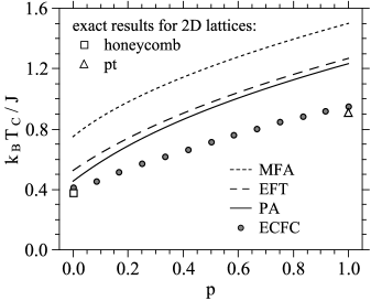
Figure 2: The Curie temperatures vs. concentration for the triangular lattice with selective dilution, obtained by various theoretical approaches: MFA, EFT, PA and ECFC for 3$\times$4 cluster. Two exact Wannier results [2] for $p=0$ and $p=1$ are also indicated.

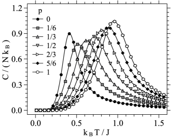
Figure 3: The specific heat per lattice site vs. temperature for various concentrations of $c$-atoms. The presented results are obtained by the ECFC method for 3$\times$4 cluster.

The Curie temperature of the pure triangular lattice is higher than that of the honeycomb one, since the coordination number of the former doubles that of the latter. It is seen in Fig. 2 that in each method the Curie temperature changes continuously with $p$; however, the change is not linear, not even in the MFA.

Fig. 2 illustrates the accuracy of the methods described in the previous Section. As far as the analytical methods are concerned, we see that MFA is the least accurate; giving the highest Curie temperature. The EFT and PA are much more accurate methods. Noticeably, the numerical calculations performed on the finite clusters with periodic boundary conditions seem to be the most accurate. As pointed out in the previous Section, in this approach the Curie temperatures have been identified from the maxima of the specific heat, according to eq. (13).

In Fig. 3 the specific heat curves per lattice site for finite clusters are illustrated vs. temperature for various concentrations $p$. The temperatures corresponding to the maxima of these curves are denoted by the circular markers in Fig. 2. Although the location of the specific heat peaks can be determined numerically from the curves, we found that the application of the analytical formula (13) leads to more precise results. It should be noted that the specific heat in Fig. 3 behaves correctly from the thermodynamic point of view, both in the low and high temperature limits.

IV Conclusions

In the paper four approximate methods have been applied in order to study the low dimensional PT Ising ferromagnet with selective dilution. Within those methods the formulas for the Curie temperatures have been obtained. The phase diagram has been calculated for various values of the concentration parameter $p$ and the results of the different methods have been compared.

The most accurate method is the one based on the exact numerical calculations for finite clusters with the periodic boundary conditions. It is worth noticing that within this method all thermodynamic properties can be simultaneously calculated in the same computational time. However, regarding the determination of the Curie temperature, this method is applicable to the systems in which the maximum of the specific heat is unambiguously related to the phase transition temperature. This is not always the case; for instance, for the frustrated systems or even some paramagnets where the so-called Schottky maximum is observed. Therefore, the analytical methods, giving better physical insight and proper interpretation of the numerical results, are still important in such studies.

Among analytical methods the PA approach can be especially recommended, for it enables the self-consistent studies of all thermodynamic properties based on the Gibbs potential. It also gives satisfactory accuracy when compared with other approaches. As shown recently, this method can be applied to the Heisenberg systems as well [24, 25]. It should also be noted that for quantum systems the numerical diagonalization of the finite cluster Hamiltonian is much less efficient than ECFC for the classical Ising model.

For the model in question the antiferromagnetic interactions can also be considered. Then, for selective dilution $p>0$ the frustrations will occur and the theoretical description becomes more complex. This problem should be a subject for separate paper.

- (1) L. Onsager, Phys. Rev. 65 (1944) 117
- (2) G. H. Wannier, Revs. Mod. Phys. 17 (1945) 50
- (3) S. Katsura, Phys. Rev. 127 (1962) 1508
- (4) N. D. Mermin, H. Wagner, Phys. Rev. Lett. 17 (1966) 1133
- (5) M. O. Elout, W. J. Maaskant, Phys. Rev. B 49 (1994) 6040
- (6) L. Čanova, J. Strečka, J. Dely, M. Jaščur, Acta Phys. Polon. A 113 (2008) 449
- (7) D.-T.-Hung, J. C. S. Levy, O. Nagai, Phys. Stat. Sol. (b) 93 (1979) 351
- (8) G. Z. Wei, A. Du, J. Magn. Magn. Matter. 127 (1993) 64
- (9) A.-Y. Hu, Y. Chen, L.-J. Peng, Physica B 393 (2007) 368
- (10) L. S. Campana, A. Caramico D’Auria, M. D’Ambrosio, U. Esposito, L. De Cesare, G. Kamieniarz, Phys. Rev B 30 (1984) 2769
- (11) R. D. Somma, A. A. Aligia, Phys. Rev. B 64 (2001) 024410
- (12) J. R. de Sousa, N. S. Branco, B. Boechat, C. Cordeiro, Physica A 328 (2003) 167
- (13) J. O. Indekeu, A. Maritan, A. L. Stella, J. Phys. A: Math. Gen. 15 (1982) L291
- (14) J. A. Plascak, W. Figueiredo, B. C. S. Grandi, Brazilian J. Phys. 29 (1999) 579
- (15) I. P. Fittipaldi, J. Magn. Magn. Mater. 131 (1994) 43
- (16) E. Rastelli, A. Tassi, L. Reatto, J. Phys. C: Solid State Phys. 7 (1974) 1735
- (17) M. Takahashi, Prog. Theoret. Phys. Suppl. 87 (1986) 233
- (18) H. Puszkarski, Phys. Rev. B 49 (1994) 6718
- (19) W. Zheng, R. R. P. Singh, R. H. McKenzie, R. Coldea, Phys. Rev. B 71 (2005) 134422
- (20) H. Betsuyaku, Solid. State Comm. 25 (1978) 185
- (21) H. Kuroyanagi, M. Matsumoto, M. Tsubota, J. Low Temp. Phys. 162 (2011) 609
- (22) M. Suzuki, M. Katori, X. Hu, J. Phys. Soc. Jpn. 56 (1987) 3092; M. Katori, M. Suzuki, ibid. 3113
- (23) G. Kamieniarz, R. Dekeyser, G. Musiał, Acta Phys. Polon. A 85 (1994) 413
- (24) T. Balcerzak, I. Łużniak, Physica A 388 (2009) 357
- (25) K. Szałowski, T. Balcerzak, Physica A 391 (2012) 2197
- (26) H. Kaya, A. N. Berker, Phys. Rev. E 62 (2000) R1469
- (27) R. Honmura, T. Kaneyoshi, J. Phys. C 12 (1979) 3979
- (28) M. Žukovič, M. Borovský, A. Bobák, Phys. Lett. A 374 (2010) 4260
- (29) A. M. Läuchli, in: Introduction to Frustrated Magnetism: Materials, Experiments, Theory, Ed. C. Lacroix, P. Mendels, F. Mila, Springer Series in Solid State Sciences, Vol. 164 (Springer, Berlin, Heidelberg 2011), p. 481
- (30) D. P. Landau, Phys. Rev. B 13 (1976) 2997
- (31) N. Jaan, O. O. Steinitz, J. Stat. Phys. 30 (1983) 37
- (32) P. H. Lundow, K. Markström, A. N. Rosengren, Philos. Mag. 89 (2009) 2009
- (33) A. M. Ferrenberg, D. P. Landau, Phys. Rev. B 44 (1991) 5081
- (34) K. Binder, Rep. Prog. Phys. 60 (1997) 487