Improved contact prediction in proteins:
Using pseudolikelihoods to infer Potts models

Abstract

Spatially proximate amino acids in a protein tend to coevolve. A protein’s 3D structure hence leaves an echo of correlations in the evolutionary record. Reverse engineering 3D structures from such correlations is an open problem in structural biology, pursued with increasing vigor as more and more protein sequences continue to fill the data banks. Within this task lies a statistical inference problem, rooted in the following: correlation between two sites in a protein sequence can arise from firsthand interaction, but can also be network-propagated via intermediate sites; observed correlation is not enough to guarantee proximity. To separate direct from indirect interactions is an instance of the general problem of inverse statistical mechanics, where the task is to learn model parameters (fields, couplings) from observables (magnetizations, correlations, samples) in large systems. In the context of protein sequences, the approach has been referred to as direct-coupling analysis. Here we show that the pseudolikelihood method, applied to 21-state Potts models describing the statistical properties of families of evolutionarily related proteins, significantly outperforms existing approaches to the direct-coupling analysis, the latter being based on standard mean-field techniques. This improved performance also relies on a modified score for the coupling strength. The results are verified using known crystal structures of specific sequence instances of various protein families. Code implementing the new method can be found at http://plmdca.csc.kth.se/.

I Introduction

In biology, new and refined experimental techniques have triggered a rapid increase in data availability during the last few years. Such progress needs to be accompanied by the development of appropriate statistical tools to treat growing data sets. An example of a branch undergoing intense growth in the amount of existing data is protein structure prediction (PSP), which, due to the strong relation between a protein’s structure and its function, is one central topic in biology. As we shall see, one can accurately estimate the 3D structure of a protein by identifying which amino-acid positions in its chain are statistically coupled over evolutionary time scales Weigt ; pmid22106262 ; journals/corr/abs-1110-5091 ; Sulkowska2012 ; Nugent . Much of the experimental output is today readily accessible through public databases such as Pfam journals/nar/PuntaCEMTBPFCCHHSEBF12 , which collects over 13,000 families of evolutionarily related protein domains, the largest of them containing more than $2\times 10^{5}$ different amino-acid sequences. Such databases allow researchers to easily access data, to extract information from it, and to confront their results.

A recurring difficulty when dealing with interacting systems is distinguishing direct interactions from interactions mediated via multi-step paths across other elements. Correlations are, in general, straightforward to compute from raw data, whereas parameters describing the true causal ties are not. The network of direct interactions can be thought of as hidden beneath observable correlations, and untwisting it is a task of inherent intricacy. In PSP, using mathematical means to dispose of the network-mediated correlations observable in alignments of evolutionarily related (and structurally conserved) proteins is necessary to get optimal results Weigt ; journals/ploscb/BurgerN10 ; Balakrishnan ; pmid22106262 ; journals/bioinformatics/JonesBCP12 and yields improvements worth the computational strain put on the analysis. This approach to PSP, which we refer to as direct-coupling analysis (DCA), is the focus of this paper.

In a more general setting, the problem of inferring interactions from observations of instances amounts to inverse statistical mechanics, a field which has been intensively pursued in statistical physics over the last decade Kappen98boltzmannmachine ; Schneidman06 ; PhysRevLett.96.030201 ; 1742-5468-2008-12-P12001 ; Frontiers ; CoccoLeiblerMonasson ; SessakMonasson ; MezardMora ; Marinari ; CoccoMonasson2011 ; Ricci-Tersenghi2012 ; Nguyen-Berg2012a ; Nguyen-Berg2012b ; 1107.3536v2 . Similar tasks were formulated earlier in statistics and machine learning, where they have been called model learning and inference hyvarinen2001independent ; rissanen2007 ; WainwrightJordan ; RavikumarWainwrightLafferty10 . To illustrate this concretely, let us start from an Ising model,

$$P(\sigma_{1},\ldots,\sigma_{N})=\frac{1}{Z}\exp{\left(\sum_{i=1}^{N}h_{i}\sigma_{i}+\sum_{1\leq i<j\leq N}J_{ij}\sigma_{i}\sigma_{j}\right)}$$ (1)

and its magnetizations $m_{i}=\partial_{h_{i}}\log Z$ and connected correlations $c_{ij}=\partial_{J_{ij}}\log Z-m_{i}m_{j}$. Counting the number of observables ($m_{i}$ and $c_{ij}$) and the number of parameters ($h_{i}$ and $J_{ij}$) it is clear that perfect knowledge of the magnetizations and correlations should suffice to determine the external fields and the couplings exactly. It is, however, also clear that such a process must be computationally expensive, since it requires the computation of the partition function $Z$ for an arbitrary set of parameters. The exact but iterative procedure known as Boltzmann machines Ackley85alearning does in fact work on small systems, but it is out of question for the problem sizes considered in this paper. On the other hand, the mean-field equations of (1) read Parisi ; Peliti ; Fischer-Hertz :

$$\tanh^{-1}m_{i}=h_{i}+\sum_{j}J_{ij}m_{j}.$$ (2)

From (2) and the fluctuation-dissipation relations an equation can be derived connecting the coupling coefficients $J_{ij}$ and the correlation matrix ${\bf c}=(c_{ij})$ Kappen98boltzmannmachine :

$$J_{ij}=-({\bf c}^{-1})_{ij}.$$ (3)

Equations (2) and (3) exemplify typical aspects of inverse statistical mechanics, and inference in large systems in general. On one hand, the parameter reconstruction using these two equations is not exact. It is only approximate, because the mean-field equations (2) are themselves only approximate. It also demands reasonably good sampling, as the matrix of correlations is not invertible unless it is of full rank, and small noise on its ${\cal O}(N^{2})$ entries may result in large errors in estimating the $J_{ij}$. On the other hand, this method is fast, as fast as inverting a matrix, because one does not need to compute $Z$. Except for mean-field methods as in (2), approximate methods recently used to solve the inverse Ising problem can be grouped as expansion in correlations and clusters SessakMonasson ; CoccoMonasson2011 , methods based on the Bethe approximation MezardMora ; Marinari ; Ricci-Tersenghi2012 ; Nguyen-Berg2012a ; Nguyen-Berg2012b , and the pseudolikelihood method RavikumarWainwrightLafferty10 ; 1107.3536v2 .

For PSP, it is not the Ising model but a 21-state Potts model which is pertinent Weigt : The model shall be learned such that it represents the statistical features of large multiple sequence alignments of homologous (evolutionarily related) proteins, and to reproduce the statistics of correlated amino acid substitutions. This can be done with the Potts equivalent of Eq. (1), i.e. using a model with pairwise interactions. As will be detailed below, strong interactions can be interpreted as indicators for spatial vicinity of residues in the three-dimensional protein fold, even if residues are well separated along the sequence – thus linking evolutionary sequence statistics with protein structure. But which of all the inference methods in inverse statistical mechanics, machine learning or statistics is most suitable for treating real protein sequence data? How do the test results obtained for independently generated equilibrium configurations of Potts models translate to the case of protein sequences, which are neither independent nor equilibrium configurations of any well-defined statistical-physics model? The main goal of this paper is to move towards an answer to this question by showing that the pseudolikelihood method is a very powerful means to perform DCA, with a prediction accuracy considerably out-performing methods previously assessed.

The paper is structured as follows: in Section II, we review the ideas underlying PSP and DCA and explain the biological hypotheses linking protein 3D structure to correlations in amino-acid sequences. We also review earlier approaches to DCA. In Section III, we describe the Potts model in the context of DCA and the properties of exponential families. We further detail a maximum-likelihood (ML) approach as brought to bear on the inverse Potts problem and discuss in more detail why this is impractical for realistic system sizes, and we introduce, similarly to (3) above, the inverse Potts mean-field model algorithm for the DCA (mfDCA) and a pseudolikelihood maximization procedure (plmDCA). This section also covers algorithmic details of both models such as regularization and sequence reweighting. A further important issue is the selection of an interaction score, which reduces coupling matrices to a scalar score, and allows for ranking of couplings according to their ’strength’. In Section IV, we present results from prediction experiments using mfDCA and plmDCA assessed against known crystal structures. In Section V, we summarize our findings, put their implications into context, and discuss possible future developments. The appendixes contain additional material supporting the main text.

II Protein Structure Prediction and Direct-Coupling Analysis

Proteins are essential players in almost all biological processes. Primarily, proteins are linear chains, each site being occupied by 1 out of 20 different amino acids. Their function relies, however, on the protein fold, which refers to the 3D conformation into which the amino-acid chain curls. This fold guarantees, e.g., that the right amino acids are exposed in the right positions at the protein surface, thus forming biochemically active sites, or that the correct pairs of amino acids are brought into contact to keep the fold thermodynamically stable.

Experimentally determining the fold, using e.g. x-ray crystallography or NMR tomography, is still a rather costly and time-consuming process. On the other hand, every newly sequenced genome results in a large number of newly predicted proteins. The number of sequenced organisms now exceeds $3,700$, and continues to grow exponentially (genomesonline.org GOLD ). The most prominent database for protein sequences, Uniprot (uniprot.org Uniprot ), lists about 25,000,000 different protein sequences, whereas the number of experimentally determined protein structures is only around 85,000 (pdb.org pdb ).

However, the situation of structural biology is not as hopeless as these numbers might suggest. First, proteins have a modular architecture; they can be subdivided into domains which, to a certain extent, fold and evolve as units. Second, domains of a common evolutionary origin, i.e., so-called homologous domains, are expected to almost share their 3D structure and to have related function. They can therefore be collected in protein domain families: the Pfam database (pfam.sanger.ac.uk journals/nar/PuntaCEMTBPFCCHHSEBF12 ) lists almost 14,000 different domain families, and the number of sequences collected in each single family ranges roughly from $10^{2}$ to $10^{5}$. In particular the larger families, with more than 1,000 members, are of interest to us, as we argue that their natural sequence variability contains important statistical information about the 3D structure of its member proteins, and can be exploited to successfully address the PSP problem.

Two types of data accessible via the Pfam database are especially important to us. The first is the multiple sequence alignment (MSA), a table of the amino acid sequences of all the protein domains in the family lined up to be as similar as possible. A (small and illustrative) example is shown in Fig. 1 (left panel). Normally, not all members of a family can be lined up perfectly, and the alignment therefore contains both amino acids and gaps. At some positions, an alignment will be highly specific (cf. the second, fully conserved column in Fig. 1), while at others it will be more variable. The second data type concerns the crystal structure of one or several members of a family. Not all families provide this second type of data. We discuss its use for an a posteriori assessment of our inference results in detail in Sec. IV.

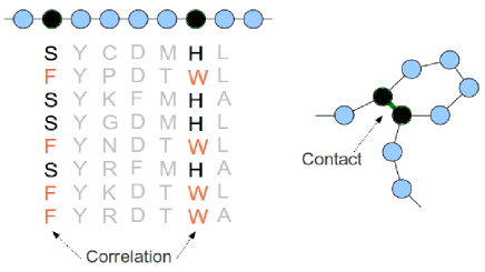
Figure 1: (Color online) Left panel: small MSA with two positions of correlated amino-acid occupancy. Right panel: hypothetical corresponding spatial conformation, bringing the two correlated positions into direct contact.

The Potts-model based inference uses only the first data type, i.e., the sequence data. Small spatial separation between amino acids in a protein, cf. the right panel of Fig. 1, encourages co-occurrence of favorable amino-acid combinations, cf. the left panel of Fig. 1. This spices the sequence record with correlations, which can be reliably determined in sufficiently large MSAs. However, the use of such correlations for predicting 3D contacts as a first step to solve the PSP problem remained of limited success pmid8208723 ; Lockless08101999 ; PROT:PROT20098 , since they can be induced both by direct interactions (amino acid $A$ is close to amino acid $B$), and by indirect interactions (amino acids $A$ and $B$ are both close to amino acid $C$). Lapedes et al. Lapedes were the first to address, in a purely theoretical setting, these ambiguities of a correlation-based route to protein sequence analysis, and these authors also outline a maximum-entropy approach to get at direct interactions. Weigt et al. Weigt successfully executed this program subsequently called direct-coupling analysis: the accuracy in predicting contacts strongly increases when direct interactions are used instead of raw correlations.

To computationally solve the task of inferring interactions in a Potts model, Weigt employed a generalization of the iterative message-passing algorithm susceptibility propagation previously developed for the inverse Ising problem MezardMora . Methods in this class are expected to outperform mean-field based reconstruction methods similar to (3) if the underlying graph of direct interactions is locally close to tree-like, an assumption which may or may not be true in a given application such as PSP. A substantial draw-back of susceptibility propagation as used in Weigt is that it requires a rather large amount of auxiliary variables, and that DCA could therefore only be carried out on protein sequences that are not too long. In pmid22106262 , this obstacle was overcome by using instead a simpler mean-field method, i.e., the generalization of (3) to a 21-state Potts model. As discussed in pmid22106262 , this broadens the reach of the DCA to practically all families currently in Pfam. It improves the computational speed by a factor of about $10^{3}$–$10^{4}$, and it appears also to be more accurate than the susceptibility-propagation based method of Weigt in predicting contact pairs. The reason behind this third advantage of mean-field over susceptibility propagation as an approximate method of DCA is unknown at this time.

Pseudolikelihood maximization (PLM) is an alternative method developed in mathematical statistics to approximate maximum-likelihood inference, which breaks down the a priori exponential time complexity of computing partition functions in exponential families besag1975 . On the inverse Ising problem it was first used by Ravikumar et al. RavikumarWainwrightLafferty10 , albeit in the context of graph sign-sparsity reconstruction; two of us showed recently that it outperforms many other approximate inverse Ising schemes on the Sherrington-Kirkpatrick model, and in several other examples 1107.3536v2 . Although this paper reports the first use of the PLM method in DCA, the idea of using pseudolikelihoods for PSP is not completely novel. Balakrishnan et al. Balakrishnan devised a version of this idea, but using a set-up rather different from that in pmid22106262 , regarding, for example, what portions of the data bases and which measures of prediction accuracy were used, and also, not couched in the language of inverse statistical mechanics. While a competitive evaluation between pmid22106262 and Balakrishnan is still open, we have not attempted such a comparison in this work.

Other ways of deducing direct interactions in PSP, not motivated from the Potts model but in somewhat similar probabilistic settings, have been suggested in the last few years. A fast method utilizing Bayesian networks was provided by Burger and van Nimwegen journals/ploscb/BurgerN10 . More recently, Jones et al. journals/bioinformatics/JonesBCP12 introduced a procedure called PSICOV (Protein Sparse Inverse COVariance). While DCA and PSICOV both appear capable of outperforming the Bayesian network approach pmid22106262 ; journals/bioinformatics/JonesBCP12 , their relative efficiency is currently open to investigation, and is not assessed in this work.

Finally, predicting amino acid contacts is not only a goal in itself, but also a means to assemble protein complexes Schug2009 ; Dago2012 and to predict full 3D protein structures journals/corr/abs-1110-5091 ; Sulkowska2012 ; Marks2012-Cell . Such tasks require additional work, using the DCA results as input, and are outside the scope of the present paper.

III Method development

III.1 The Potts model

Let $\boldsymbol{\sigma}=(\sigma_{1},\sigma_{2},\cdots,\sigma_{N})$ represent the amino acid sequence of a domain with length $N$. Each $\sigma_{i}$ takes on values in $\{1,2,...,q\}$, with $q=21$: one state for each of the 20 naturally occurring amino acids and one additional state to represent gaps. Thus, an MSA with $B$ aligned sequences from a domain family can be written as an integer array $\{\boldsymbol{\sigma}^{(b)}\}^{B}_{b=1}$, with one row per sequence and one column per chain position. Given an MSA, the empirical individual and pairwise frequencies can be calculated as

$$f_{i}(k) = \frac{1}{B}\sum^{B}_{b=1}\delta(\sigma^{(b)}_{i},k),$$

$$f_{ij}(k,l) = \frac{1}{B}\sum^{B}_{b=1}\delta(\sigma^{(b)}_{i},k)\ \delta(\sigma^{(b)}_{j},l),$$ (4)

where $\delta(a,b)$ is the Kronecker symbol taking value 1 if both arguments are equal, and 0 otherwise. $f_{i}(k)$ is hence the fraction of sequences for which the entry on position $i$ is amino acid $k$, gaps counted as a 21st amino acid. Similarly, $f_{ij}(k,l)$ is the fraction of sequences in which the position pair $(i,j)$ holds the amino acid combination $(k,l)$. Connected correlations are given as

$$c_{ij}(k,l)=f_{ij}(k,l)-f_{i}(k)\,f_{j}(l).$$ (5)

A (generalized) Potts model is the simplest probabilistic model $P(\boldsymbol{\sigma})$ which can reproduce the empirically observed $f_{i}(k)$ and $f_{ij}(k,l)$. In analogy to (1) it is defined as

$$P(\boldsymbol{\sigma})=\frac{1}{Z}\exp\left(\sum\limits^{N}_{i=1}{h_{i}(\sigma_{i})}+\sum_{1\leq i<j\leq N}{J_{ij}(\sigma_{i},\sigma_{j})}\right),$$ (6)

in which $h_{i}(\sigma_{i})$ and $J_{ij}(\sigma_{i},\sigma_{j})$ are parameters to be determined through the constraints

$$P(\sigma_{i}=k) = \sum\limits_{\underset{\sigma_{i}=k}{\boldsymbol{\sigma}}}P(\boldsymbol{\sigma})=f_{i}(k),$$

$$P(\sigma_{i}=k,\sigma_{j}=l) = \sum\limits_{\underset{\underset{\sigma_{i}=k}{\sigma_{j}=l}}{\boldsymbol{\sigma}}}P(\boldsymbol{\sigma})=f_{ij}(k,l).$$ (7)

It is immediate that the probabilistic model which maximizes the entropy while satisfying Eq. (III.1) must take the Potts model form. Finding a Potts model which matches empirical frequencies and correlations is therefore referred to as a maximum-entropy inference jaynes57a ; jaynes57b , cf. also Lapedes ; Weigt for a formulation in terms of protein-sequence modeling.

On the other hand, we can use Eq. (6) as a variational ansatz and maximize the probability of the input data set $\{\boldsymbol{\sigma}^{(b)}\}^{B}_{b=1}$ with respect to the model parameters $h_{i}(\sigma)$ and $J_{ij}(\sigma,\sigma^{\prime})$; this maximum-likelihood perspective is used in the following. We note that the Ising and the Potts models (and most models which are normally considered in statistical mechanics) are examples of exponential families, and have the property that means and correlations are sufficient statistics darmois35 ; pitman-wishart36 ; koopman36 . Given unlimited computing power to determine $Z$, reconstruction can not be done better using all the data compared to using only (empirical) means and (empirical) correlations. It is only when one cannot compute $Z$ exactly and has to resort to approximate methods, that using directly all the data can bring any advantage.

III.2 Model parameters and gauge invariance

The total number of parameters of Eq, (6) is $Nq+\frac{N(N-1)}{2}q^{2}$, but, in fact, the model as it stands is overparameterized in the sense that distinct parameter sets can describe the same probability distribution. It is easy to see that the number of nonredundant parameters is $N(q-1)+\frac{N(N-1)}{2}(q-1)^{2}$, cf. an Ising model ($q=2$), which has $\frac{N(N+1)}{2}$ parameters if written as in Eq. (1) but would have $2N^{2}$ parameters if written in the form of Eq. (6).

A gauge choice for the Potts model, which eliminates the overparametrization in a similar manner as in the Ising model (and reduces to that case for $q=2$), is

$$\sum_{s=1}^{q}J_{ij}(k,s)=\sum_{s=1}^{q}J_{ij}(s,l)=\sum_{s=1}^{q}h_{i}(s)=0,$$ (8)

for all $i$, $j(>i)$, $k$, and $l$. Alternatively, we can choose a gauge where one index, say $i=q$, is special, and measure all interaction energies with respect to this value, i.e.,

$$J_{ij}(q,l)=J_{ij}(k,q)=h_{i}(q)=0,$$ (9)

for all $i$, $j(>i)$, $k$, and $l$, cf. pmid22106262 . This gauge choice corresponds to a lattice gas model with $q-1$ different particle types, and a maximum occupation number one.

Using either (8) or (9) reconstruction is well-defined, and it is straight-forward to translate results obtained in one gauge to the other.

III.3 The inverse Potts problem

Given a set of independent equilibrium configurations $\{\boldsymbol{\sigma}^{(b)}\}^{B}_{b=1}$ of the model Eq. (6), the ordinary statistical approach to inferring parameters $\{\boldsymbol{\mathrm{h}},\boldsymbol{\mathrm{J}}\}$ would be to let those parameters maximize the likelihood (i.e., the probability of generating the data set for a given set of parameters). This is equivalent to minimizing the (rescaled) negative log-likelihood function

$$l=-\frac{1}{B}\sum\limits^{B}_{b=1}\log P(\boldsymbol{\sigma}^{(b)}).$$ (10)

For the Potts model (6), this becomes

$$l(\boldsymbol{\mathrm{h}},\boldsymbol{\mathrm{J}}) = \log Z-\sum\limits^{N}_{i=1}\sum\limits^{q}_{k=1}{f_{i}(k)h_{i}(k)}$$

$$-\sum_{1\leq i<j\leq N}\sum\limits^{q}_{k,l=1}{f_{ij}(k,l)J_{ij}(k,l)}.$$

$l$ is differentiable, so minimizing it means looking for a point at which $\partial_{h_{i}(k)}l=0$ and $\partial_{J_{ij}(k,l)}l=0$. Hence, ML estimates will satisfy

$$\partial_{h_{i}(k)}\log Z-f_{i}(k) = 0,$$

$$\partial_{J_{ij}(k,l)}\log Z-f_{ij}(k,l) = 0.$$ (12)

To achieve this minimization computationally, we need to be able to calculate the partition function $Z$ of Eq. (6) for any realization of the parameters $\{\boldsymbol{\mathrm{h}},\boldsymbol{\mathrm{J}}\}$. This problem is computationally intractable for any reasonable system size. Approximate minimization is essential, and we will show that even relatively simple approximation schemes lead to accurate PSP results.

III.4 Naive mean-field inversion

The mfDCA algorithm in pmid22106262 is based on the simplest and computationally most efficient approximation, i.e.,  naive mean-field inversion (NMFI). It starts from the proper generalization of (2), cf. Kholodenko1990 , and then uses linear response: The $J$’s in the lattice-gas gauge Eq. (9) become:

$$J^{NMFI}_{ij}(k,l)=-({\boldsymbol{\mathrm{C}}}^{-1})_{ab},$$ (13)

where $a=(q-1)(i-1)+k$ and $b=(q-1)(j-1)+l$. The matrix $\boldsymbol{\mathrm{C}}$ is the $N(q-1)\times N(q-1)$ covariance matrix assembled by joining the $N(q-1)\times N(q-1)$ values $c_{ij}(k,l)$ as defined in Eq. (5), but leaving out the last state $q$. In Eq. (13), $i,j\in\{1,...,N\}$ are site indices, and $k,l$ run from $1$ to $q-1$. Under gauge Eq. (9), all the other coupling parameters are zero. The term ’naive’ has become customary in the inverse statistical mechanics literature, often used to highlight the difference to a Thouless-Anderson-Palmer level inversion or one based on the Bethe approximation. The original meaning of this term lies, as far as we are aware, in information geometry Tanaka2000 ; amari2001 .

III.5 Pseudolikelihood maximization

Pseudolikelihood substitutes the probability in (10) by the conditional probability of observing one variable $\sigma_{r}$ given observations of all the other variables $\boldsymbol{\sigma}_{\backslash r}$. That is, the starting point is

$$P(\sigma_{r} = \sigma_{r}^{(b)}|\boldsymbol{\sigma}_{\backslash r}=\boldsymbol{\sigma}_{\backslash r}^{(b)})$$ (14)

$$= \frac{\exp\left(h_{r}(\sigma_{r}^{(b)})+\sum\limits^{N}_{\underset{i\neq r}{i=1}}{J_{ri}(\sigma_{r}^{(b)},\sigma_{i}^{(b)})}\right)}{\sum_{l=1}^{q}\exp\left(h_{r}(l)+\sum\limits^{N}_{\underset{i\neq r}{i=1}}{J_{ri}(l,\sigma_{i}^{(b)})}\right)},$$

where, for notational convenience, we take $J_{ri}(l,k)$ to mean $J_{ir}(k,l)$ when $i<r$. Given an MSA, we can maximize the conditional likelihood by minimizing

$$g_{r}(\boldsymbol{\mathrm{h}}_{r},\boldsymbol{\mathrm{J}}_{r})=-\frac{1}{B}\sum\limits^{B}_{b=1}\log\left[P_{\{\boldsymbol{\mathrm{h}}_{r},\boldsymbol{\mathrm{J}}_{r}\}}(\sigma_{r}=\sigma^{(b)}_{r}|\boldsymbol{\sigma}_{\backslash r}=\boldsymbol{\sigma}^{(b)}_{\backslash r})\right].$$ (15)

Note that this only depends on $\boldsymbol{\mathrm{h}}_{r}$ and $\boldsymbol{\mathrm{J}}_{r}=\{\boldsymbol{\mathrm{J}}_{ir}\}_{i\neq r}$, i.e., on the parameters featuring node $r$. If (15) is used for all $r$ this leads to unique values for the parameters $\boldsymbol{\mathrm{h}}_{r}$ but typically different predictions for $\boldsymbol{\mathrm{J}}_{rq}$ and $\boldsymbol{\mathrm{J}}_{qr}$ (which should be the same). Minimizing (15) must therefore be supplemented by some procedure on how to reconcile different values of $\boldsymbol{\mathrm{J}}_{rq}$ and $\boldsymbol{\mathrm{J}}_{qr}$; one way would be to simply use their average $\frac{1}{2}({\boldsymbol{\mathrm{J}}_{rq}+\boldsymbol{\mathrm{J}}_{qr}^{T}})$ RavikumarWainwrightLafferty10 .

We here reconcile different $\boldsymbol{\mathrm{J}}_{rq}$ and $\boldsymbol{\mathrm{J}}_{qr}$ by minimizing an objective function adding $g_{r}$ for all nodes:

$$l_{pseudo}(\boldsymbol{\mathrm{h}},\boldsymbol{\mathrm{J}})=\sum\limits^{N}_{r=1}g_{r}(\boldsymbol{\mathrm{h}}_{r},\boldsymbol{\mathrm{J}}_{r})$$

$$= -\frac{1}{B}\sum\limits^{N}_{r=1}\sum\limits^{B}_{b=1}\log\left[P_{\{\boldsymbol{\mathrm{h}}_{r},\boldsymbol{\mathrm{J}}_{r}\}}(\sigma_{r}=\sigma^{(b)}_{r}|\boldsymbol{\sigma}_{\backslash r}=\boldsymbol{\sigma}^{(b)}_{\backslash r})\right].$$

Minimizers of $l_{pseudo}$ generally do not minimize $l$; the replacement of likelihood with pseudolikelihood alters the outcome. Note, however, that replacing $l$ by $l_{pseudo}$ resolves the computational intractability of the parameter optimization problem: instead of depending on the full partition function, the normalization of the conditional probability (14) contains only a single summation over the $q=21$ Potts states. The intractable average over the $N-1$ conditioning spin variables is replaced by an empirical average over the data set in Eq. (III.5).

III.6 Regularization

A Potts model describing a protein family with sequences of 50-300 amino acids requires ca. $5\cdot 10^{5}$ to $2\cdot 10^{7}$ parameters. At present, few protein families are in this range in size, and regularization is therefore needed to avoid overfitting. In NMFI, the problem results in an empirical covariance matrix which typically is not of full rank, and Eq. (13) is not well-defined. In pmid22106262 , one of the authors therefore used the pseudocount method where frequencies and empirical correlations are adjusted using a regularization variable $\lambda$:

$$f_{i}(k) = \frac{1}{\lambda+B}\left[\frac{\lambda}{q}+\sum^{B}_{b=1}\delta(\sigma^{(b)}_{i},k)\right],$$ (17)

$$f_{ij}(k,l) = \frac{1}{\lambda+B}\left[\frac{\lambda}{q^{2}}+\sum^{B}_{b=1}\delta(\sigma^{(b)}_{i},k)\ \delta(\sigma^{(b)}_{j},l)\right].$$

The pseudocount is a proxy for many observations, which – if they existed – would increase the rank of the correlation matrix; the pseudocount method hence promotes invertibility of the matrix in Eq. (13). It was observed in pmid22106262 that for good performance in DCA, the pseudocount parameter $\lambda$ has to be taken fairly large, on the order of $B$.

In the PLM method, we take the standard route of adding a penalty term to the objective function:

$$\{\boldsymbol{\mathrm{h}}^{PLM},\boldsymbol{\mathrm{J}}^{PLM}\}=\underset{\{\boldsymbol{\mathrm{h}},\boldsymbol{\mathrm{J}}\}}{\mathrm{argmin}}\{l_{pseudo}(\boldsymbol{\mathrm{h}},\boldsymbol{\mathrm{J}})+R(\boldsymbol{\mathrm{h}},\boldsymbol{\mathrm{J}})\}.$$ (18)

The turnout is then a trade-off between likelihood maximization and whatever qualities $R$ is pushing for. Ravikumar et al. RavikumarWainwrightLafferty10 pioneered the use of $l_{1}$ regularizers for the inverse Ising problem, which forces a fraction of parameters to assume value zero, thus effectively reducing the number of parameters. This approach is not appropriate here since we are concerned with the accuracy (resp. divergence) of the strongest predicted couplings; for our purposes it makes no substantial difference whether weak couplings are inferred to be small or set precisely to 0. Our choice for $R$ is therefore the simpler $l_{2}$ norm

$$R_{l_{2}}(\boldsymbol{\mathrm{h}},\boldsymbol{\mathrm{J}})=\lambda_{h}\sum\limits^{N}_{r=1}||\boldsymbol{\mathrm{h}}_{r}||^{2}_{2}+\lambda_{J}\sum_{1\leq i<j\leq N}||\boldsymbol{\mathrm{J}}_{ij}||^{2}_{2},$$ (19)

using two regularization parameters $\lambda_{h}$ and $\lambda_{J}$ for field and coupling parameters. An advantage of a regularizer is that it eliminates the need to fix a gauge, since among all parameter sets related by a gauge transformation, i.e., all parameter sets resulting in the same Potts model, there will be exactly one set which minimizes the strictly convex regularizer. For the case of the $l_{2}$ norm, it can be shown that this leads to a gauge where $\sum_{s=1}^{q}J_{ij}(k,s)=\frac{\lambda_{h}}{\lambda_{J}}h_{i}(k)$, $\sum_{s=1}^{q}J_{ij}(s,l)=\frac{\lambda_{h}}{\lambda_{J}}h_{j}(l)$, and $\sum_{s=1}^{q}h_{i}(s)=0$ for all $i$, $j(>i)$, $k$, and $l$.

To summarize this discussion: For NMFI, we regularize with pseudocounts under the gauge constraints Eq. (9). For PLM, we regularize with $R_{l_{2}}$ under the full parametrization.

III.7 Sequence reweighting

Maximum-likelihood inference of Potts models relies – as discussed above – on the assumption that the $B$ sample configurations in our data set are independently generated from Eq. (6). This assumption is not correct for biological sequence data, which have a phylogenetic bias. In particular, in the databases there are many protein sequences from related species, which did not have enough time of independent evolution to reach statistical independence. Furthermore, the selection of sequenced species in the genomic databases is dictated by human interest, and not by the aim to have an as independent as possible sampling in the space of all functional amino-acid sequences. A way to mitigate effects of uneven sampling, employed in pmid22106262 , is to equip each sequence $\boldsymbol{\sigma}^{(b)}$ with a weight $w_{b}$ which regulates its impact on the parameter estimates. Sequences deemed unworthy of independent-sample status (too similar to other sequences) can then have their weight lowered, whereas sequences which are quite different from all other sequences will contribute with a higher weight to the amino-acid statistics.

A simple but efficient way (cf. pmid22106262 ) is to measure the similarity $\hbox{sim}(\boldsymbol{\sigma}^{(a)},\boldsymbol{\sigma}^{(b)})$ of two sequences $\boldsymbol{\sigma}^{(a)}$ and $\boldsymbol{\sigma}^{(b)}$ as the fraction of conserved positions (i.e., identical amino acids), and compare this fraction to a preselected threshold $x$ , $0<x<1$. The weight given to a sequence $\boldsymbol{\sigma}^{(b)}$ can then be set to $w_{b}=\frac{1}{m_{b}}$, where $m_{b}$ is the number of sequences in the MSA similar to $\boldsymbol{\sigma}^{(b)}$:

$$m_{b}=|\{a\in\{1,...,B\}:\hbox{sim}(\boldsymbol{\sigma}^{(a)},\boldsymbol{\sigma}^{(b)})\geq x\}|.$$ (20)

In pmid22106262 , a suitable threshold $x$ was found to be $0.8$, results only weakly dependent on this choice throughout $0.7<x<0.9$. We have here followed the same procedure using threshold $x=0.9$. The corresponding reweighted frequency counts then become

$$f_{i}(k) = \frac{1}{\lambda+B_{eff}}\left[\frac{\lambda}{q}+\sum^{B}_{b=1}w_{b}\,\delta(\sigma^{(b)}_{i},k)\right],$$ (21)

$$f_{ij}(k,l) = \frac{1}{\lambda+B_{eff}}\left[\frac{\lambda}{q^{2}}+\sum^{B}_{b=1}w_{b}\,\delta(\sigma^{(b)}_{i},k)\,\delta(\sigma^{(b)}_{j},l)\right],$$

where $B_{eff}=\sum^{B}_{b=1}w_{b}$ becomes a measure of the number of effectively nonredundant sequences.

In the pseudolikelihood we use the direct analog of Eq. (21), i.e.,

$$l_{pseudo}(\boldsymbol{\mathrm{h}},\boldsymbol{\mathrm{J}})$$

$$= \!-\frac{1}{B_{eff}}\!\sum\limits^{B}_{b=1}\!w_{b}\!\sum\limits^{N}_{r=1}\log\left[P_{\{\boldsymbol{\mathrm{h}}_{r},\boldsymbol{\mathrm{J}}_{r}\}}(\sigma_{r}=\sigma^{(b)}_{r}|\boldsymbol{\sigma}_{\backslash r}=\boldsymbol{\sigma}^{(b)}_{\backslash r})\right].$$

As in the frequency counts, each sequence is considered to contribute a weight $w_{b}$, instead of the standard weight one used in i.i.d. samples.

III.8 Interaction scores

In the inverse Ising problem, each interaction is scored by one scalar coupling strength $J_{ij}$. These can easily be ordered, e.g. by absolute size. In the inverse Potts problem, each position pair $(i,j)$ is characterized by a whole $q\times q$ matrix $\boldsymbol{\mathrm{J}}_{ij}$, and some scalar score $\mathcal{S}_{ij}$ is needed in order to evaluate the ‘coupling strength’ of two sites.

In Weigt and pmid22106262 the score used is based on direct information (DI), i.e., the mutual information of a restricted probability model not including any indirect coupling effects between the two positions to be scored. Its construction goes as follows: For each position pair $(i,j)$, (the estimate of) $\boldsymbol{\mathrm{J}}_{ij}$ is used to set up a ’direct distribution’ involving only nodes $i$ and $j$,

$$P^{(dir)}_{ij}(k,l)\sim\exp\left(J_{ij}(k,l)+h^{\prime}_{i,k}+h^{\prime}_{j,l}\right).$$ (23)

$h^{\prime}_{i,k}$ and $h^{\prime}_{j,l}$ are new fields, computed as to ensure agreement of the marginal single-site distributions with the empirical individual frequency counts $f_{i}(k)$ and $f_{j}(l)$. The score $\mathcal{S}_{ij}^{DI}$ is now calculated as the mutual information of $P^{(dir)}$:

$$\mathcal{S}_{ij}^{DI}=\sum\limits^{q}_{k,l=1}P^{(dir)}_{ij}(k,l)\log\left(\frac{P^{(dir)}_{ij}(k,l)}{f_{i}(k)\,f_{j}(l)}\right).$$ (24)

A nice characteristic of $\mathcal{S}_{ij}^{DI}$ is its invariance with respect to the gauge freedom of the Potts model, i.e., both choices Eqs. (8) and (9) (or any other valid choice) generate identical $\mathcal{S}_{ij}^{DI}$.

In the pseudolikelihood approach, we prefer not to use $\mathcal{S}_{ij}^{DI}$, as this would require a pseudocount $\lambda$ to regularize the frequencies in (24), introducing a third regularization variable in addition to $\lambda_{h}$ and $\lambda_{J}$. Another possible scoring function, already mentioned but not used in Weigt , is the Frobenius norm (FN)

$$\|{\boldsymbol{\mathrm{J}}_{ij}}\|_{2}=\sqrt{\sum\limits^{q}_{k,l=1}J_{ij}(k,l)^{2}}.$$ (25)

Unlike $\mathcal{S}_{ij}^{DI}$, (25) is not independent of gauge choice, so one must be a bit careful. As was noted in Weigt , the zero sum gauge (8) minimizes the Frobenius norm, in a sense making (8) the most appropriate gauge choice for the score (25). Recall from above that our pseudolikelihood uses the full representation and fixes the gauge by the regularization terms $R_{l_{2}}$. Our procedure is therefore to first infer the interaction parameters using the pseudolikelihood and the regularization, and then to change to the zero-sum gauge:

$$J^{\prime}_{ij}(k,l)=J_{ij}(k,l)-J_{ij}(\cdot,l)-J_{ij}(k,\cdot)+J_{ij}(\cdot,\cdot),$$ (26)

where ‘$\cdot$’ denotes average over the concerned position. One can show that (26) preserves the probabilities of (6) (after altering the fields appropriately) and that $J^{\prime}_{ij}(k,l)$ satisfy (8). A possible Frobenius norm score is hence

$$\mathcal{S}_{ij}^{FN}=\|{\boldsymbol{\mathrm{J}}^{\prime}_{ij}}\|_{2}=\sqrt{\sum\limits^{q}_{k,l=1}J^{\prime}_{ij}(k,l)^{2}}.$$ (27)

Lastly, we borrow an idea from Jones et al. journals/bioinformatics/JonesBCP12 , whose PSICOV method also uses a norm rank ($1$-norm instead of Frobenius norm), but adjusted by an average-product correction (APC) term. APC was introduced in journals/bioinformatics/DunnWG08 to suppress effects from phylogenetic bias and insufficient sampling. Incorporating also this correction, we have our scoring function

$$\mathcal{S}_{ij}^{CN}=\mathcal{S}_{ij}^{FN}-\frac{\mathcal{S}_{\cdot j}^{FN}\mathcal{S}_{i\cdot}^{FN}}{\mathcal{S}_{\cdot\cdot}^{FN}},$$ (28)

where CN stands for ‘corrected norm’. An implementation of plmDCA in MATLAB is available at http://plmdca.csc.kth.se/.

IV Evaluating the performance of mfDCA and plmDCA across protein families

We have performed numerical experiments using mfDCA and plmDCA on a number of domain families from the Pfam database; here we report and discuss the results.

IV.1 Domain families, native structures, and true-positive rates

The speed of mfDCA enabled Morcos et al. pmid22106262 to conduct a large-scale analysis using 131 families. PLM is computationally more demanding than NMFI, so we chose to start with a smaller collection of 17 families, listed in Table 1. To ease the numerical effort, we chose families with relatively small $N$ and $B$. More precisely, we selected families out of the first 115 Pfam entries (low Pfam ID), which have (i) at most $N=130$ residues, (ii) between 2,000 and 22,000 sequences, and (iii) reliable structural information (cf. the PDB entries provided in the table). No selection based on DCA performance was done. In the appendix, a number of longer proteins is studied. The mfDCA performance on the selected families was found to be coherent with the larger data set of Morcos et al..

Family ID	$N$	$B$	$B_{eff}$ (90%)	PDB ID	UniProt entry	UniProt residues
PF00011	102	5024	3481	2bol	TSP36_TAESA	106-206
PF00013	58	6059	3785	1wvn	PCBP1_HUMAN	281-343
PF00014	53	2393	1812	5pti	BPT1_BOVIN	39-91
PF00017	77	2732	1741	1o47	SRC_HUMAN	151-233
PF00018	48	5073	3354	2hda	YES_HUMAN	97-144
PF00027	91	12129	9036	3fhi	KAP0_BOVIN	154-238
PF00028	93	12628	8317	2o72	CADH1_HUMAN	267-366
PF00035	67	3093	2254	1o0w	RNC_THEMA	169-235
PF00041	85	15551	10631	1bqu	IL6RB_HUMAN	223-311
PF00043	95	6818	5141	6gsu	GSTM1_RAT	104-192
PF00046	57	7372	3314	2vi6	NANOG_MOUSE	97-153
PF00076	70	21125	14125	1g2e	ELAV4_HUMAN	48-118
PF00081	82	3229	1510	3bfr	SODM_YEAST	27-115
PF00084	56	5831	4345	1elv	C1S_HUMAN	359-421
PF00105	70	2549	1277	1gdc	GCR_RAT	438-507
PF00107	130	17864	12114	1a71	ADH1E_HORSE	203-338
PF00111	78	7848	5805	1a70	FER1_SPIOL	58-132

Table 1: Domain families included in our study, listed with Pfam ID, length $N$, number of sequences $B$ (after removal of duplicate sequences), number of effective sequences $B_{eff}$ (under $x=0.9$, i.e., $90\%$ threshold for reweighting), and the PDB and UniProt specifications for the structure used to access the DCA prediction quality.

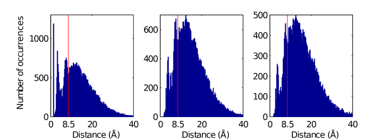
Figure 2: (Color online) Histograms of crystal-structure distances pooled from all 17 families, when including all pairs (left), pairs with $|j-i|>4$ (center), and pairs with $|j-i|>14$ (right). The vertical line is our contact cutoff 8.5Å.

To reliably assess how good a contact prediction is, something to regard as a ’gold standard’ is helpful. For each of the 17 families we have therefore selected one representative high-resolution X-ray crystal structure (resolution below 3Å), see Table 1 for the corresponding PDB identification.

From these native protein structures, we have extracted position-position distances $d(i,j)$ for each pair of sequence positions, by measuring the minimal distance between any two heavy atoms belonging to the amino acids present in these positions. The left panel of Fig. 2 shows the distribution of these distances in all considered families. Three peaks protrude from the background distribution: one at small distances below 1.5Å, a second at about 3-5Å and a third at about 7-8Å. The first peak corresponds to the peptide bonds between sequence neighbors, whereas the other two peaks correspond to nontrivial contacts between amino acids, which may be distant along the protein backbone, as can be seen from the center and right panels of Fig. 2, which collect only distances between positions $i$ and $j$ with minimal separation $|j-i|\geq 5$ resp. $|j-i|\geq 15$. Following pmid22106262 , we take the peak at 3-5Å to presumably correspond to short-range interactions like hydrogen bonds or secondary-structure contacts, whereas the last peak likely corresponds to long-range, possibly water-mediated interactions. These peaks contain the nontrivial information we would like to extract from sequence data using DCA. In order to accept the full second peak, we have chosen a distance cutoff of 8.5Å for true contacts, slightly larger than the value of 8Å used in pmid22106262 .

Accuracy results are here reported primarily using true-positive (TP) rates, also the principal measurement in pmid22106262 and journals/bioinformatics/JonesBCP12 . The TP rate for $p$ is the fraction of the $p$ strongest-scored pairs which are actually contacts in the crystal structure, defined as described above. To exemplify TP rates, let us jump ahead and look at Fig. 3. For PLM and protein family PF00076, the TP rate is 1 up to $p=80$, which means that all 80 top-$\mathcal{S}_{ij}^{CN}$ pairs are genuine contacts in the crystal structure. At $p=200$, the TP rate has dropped to 0.78, so $0.78\cdot 200=156$ of the top 200 top-$\mathcal{S}_{ij}^{CN}$ pairs are contacts, while 44 are not.

IV.2 Parameter settings

To set the stage for comparison, we started by running initial trials on the 17 families using both NMFI and PLM with many different regularization and reweighting strengths. Reweighting indeed raised the TP rates, and, as reported in pmid22106262 for 131 families, results seemed robust toward the exact choice of the limit $x$ around $0.7\leq x\leq 0.9$. We chose $x=0.9$ to use throughout the study.

In what follows, NMFI results are reported using the same list of pseudocounts as in Fig. S11 in pmid22106262 : $\lambda=w\cdot B_{eff}$ with $w=\{0.11$, $0.25$, $0.43$, $0.67$, $1.0$, $1.5$, $2.3$, $4.0$, $9.0\}$. During our analysis we also ran intermediate values, and we found this covering to be sufficiently dense. We give outputs from two versions of NMFI: NMFI-DI and NMFI-DI(true). The former uses pseudocounts for all calculations, whereas the latter switches to true frequencies when it gets to the evaluations of $\mathcal{S}_{ij}^{DI}$. We append ’DI’ to the NMFI name, since, later on, we will also try the $\mathcal{S}_{ij}^{CN}$ score for NMFI (which we will call NMFI-CN).

With $l_{2}$ regularization in the PLM algorithm, outcomes were robust against the precise choice of $\lambda_{h}$; TP rates were almost identical when $\lambda_{h}$ was changed between $0.001$ and $0.1$. We therefore chose $\lambda_{h}=0.01$ for all experiments. What mattered, rather, was the coupling regularization parameters $\lambda_{J}$, for which we did a systematic scan from $\lambda_{J}=0$ and up using step-size 0.005.

So, to summarize, the results reported here are based on $x=0.9$, cutoff 8.5Å, $\lambda_{h}=0.01$, and $\lambda$ and $\lambda_{J}$ drawn from collections of values as described above.

IV.3 Main comparison of mfDCA and plmDCA

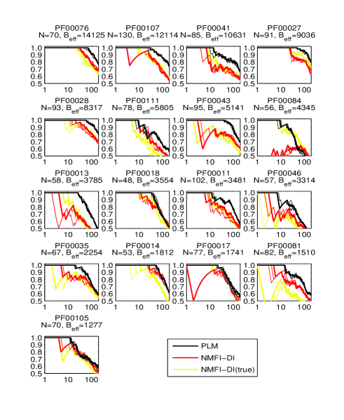
Figure 3: (Color online) Contact-detection results for the 17 families, sorted by $B_{eff}$. The y-axes are TP rates and x-axes are the number of predicted contacts $p$, based on pairs with $|j-i|>4$. The three curves for each method are the three regularization levels yielding highest TP rates across all families. The thickened curve highlights the best one out of these three ($\lambda=B_{eff}$ for NMFI and $\lambda_{J}=0.01$ for PLM).

Fig. 3 shows TP rates for the different families and methods. We see that the TP rates of plmDCA (PLM) are consistently higher than those of mfDCA (NMFI), especially for families with large $B_{eff}$. For what concerns the two NMFI versions: NMFI-DI(true) avoids the strong failure seen in NMFI-DI for PF00084, but for most other families, see in particular PF00014 and PF00081, the performance instead drops using marginals without pseudocounts in the $\mathcal{S}_{ij}^{DI}$ calculation. For both NMFI-DI and NMFI-DI(true), the best regularization was found to be $\lambda=1\cdot B_{eff}$, the same value as used in pmid22106262 . For PLM, the best parameter choice was $\lambda_{J}=0.01$. Interestingly, this same regularization parameter was optimal for basically all families. This is somewhat surprising, since both $N$ and $B_{eff}$ span quite wide ranges ($48$-$130$ and $1277$-$14125$ respectively).

In the following discussion, we leave out all results for NMFI-DI(true) and focus on PLM vs. NMFI-DI, i.e., the version used in pmid22106262 . All plots remaining in this section use the optimal regularization values: $\lambda=B_{eff}$ for NMFI and $\lambda_{J}=0.01$ for PLM.

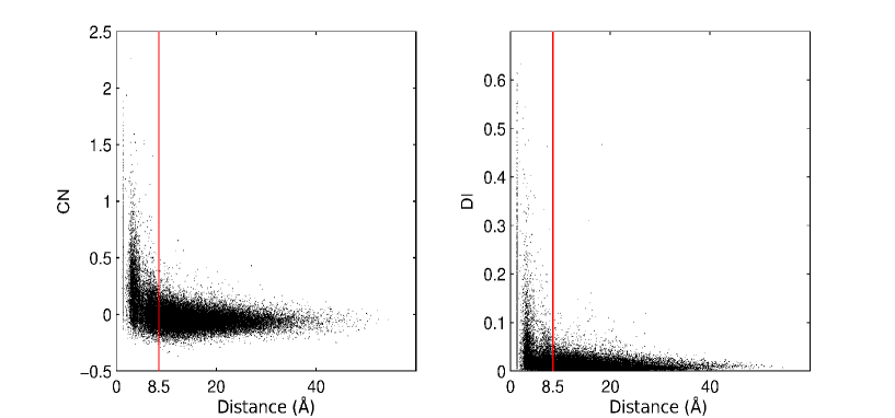
Figure 4: (Color online) Score plotted against distance for all position pairs in all 17 families for PLM (left) and NMFI-DI (right). The vertical line is our contact cutoff at 8.5Å.

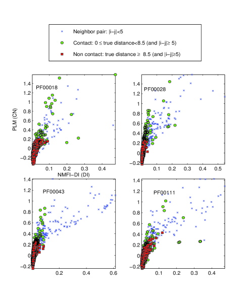
Figure 5: (Color online) Scatter plots of interaction scores for PLM and NMFI-DI from four families. For all plots, the axes are as indicated by the top left figure. The distance unit in the top box is Å.

Figure 6: (Color online) Predicted contact maps for PLM (right part, black symbols) and NMFI-DI (left part, red symbols online) for four families. A pair $(i,j)$’s placement in the plots is found by matching positions $i$ and $j$ on the axes. Native contacts are indicated in gray. True and false positives are represented by circles and crosses, respectively. Each figure shows the $1.5N$ strongest ranked pairs (including neighbors) for that family.

TP rates only classify pairs as contacts ($d(i,j)<8.5$Å) or noncontacts ($d(i,j)\geq 8.5$Å). To give a more detailed view of how scores correlate with spatial separation, we show in Fig. 4 a scatter plot of the score vs. distance for all pairs in all 17 families. PLM and NMFI-DI both manage to detect the peaks seen in the true distance distribution of Fig. 2, in the sense that high scores are observed almost exclusively at distances below 8.5Å. Both methods agree that interactions get, on average, progressively weaker going from peak one, to two, to three, and finally to the bulk. We note that the dots scatter differently across the PLM and NMFI-DI figures, reflecting the two separate scoring techniques: $\mathcal{S}_{ij}^{DI}$ are strictly nonnegative, whereas APC corrected norms can assume negative values. We also observe how sparse the extracted signal is: most spatially close pairs do not show elevated scores. However, from the other side, almost all strongly coupled pairs are close, so the biological hypothesis of Sec. II is well supported here.

Fig. 5 shows scatter plots of scores for PLM and NMFI-DI for some selected families. Qualitatively the same patterns were observed for all families. The points are clearly correlated, so, to some extent, PLM and NMFI-DI agree on the interaction strengths. Due to the different scoring schemes, we would not expect numerical coincidence of scores. Many of PLM’s top-scoring position pairs have also top scores for NMFI-DI and vice versa. The largest discrepancy is in how much more strongly NMFI-DI responds to pairs with small $|j-i|$; the crosses tend to shoot out to the right. PLM agrees that many of these neighbor pairs interact strongly, but, unlike NMFI-DI, it also shows rivaling strengths for many $|j-i|>4$-pairs.

An even more detailed picture is given by considering contact maps, see Fig. 6. The tendency observed in the last scatter plots remains: NMFI-DI has a larger portion of highly scored pairs in the neighbor zone, which are the middle stretches in these figures. An important observation is, however, that clusters of contacting pairs with long 1D sequence separation are captured by both algorithms.

Note, that only a relatively small fraction of contacts is uncovered by DCA, before false positives start to appear, and that many native contacts are missed. However, the aim of DCA cannot be to reproduce a complete contact map: It is based on sequence correlations alone (e.g. it cannot predict contacts for 100% conserved residues), it does not consider any physico-chemical property of amino acids (they are seen as abstract letters), it does not consider the need to be embeddable in 3D. Furthermore, proteins may undergo conformational changes (e.g. allostery) or homo-dimerize, so coevolution may be induced by pairs which are not in contact in the X-ray crystal structure used for evaluating prediction accuracy. The important point – and this seems to be a distinguishing feature of maximum-entropy models as compared to simpler correlation-based methods – is to find a sufficient number of well-distributed contacts to enable de-novo 3D structure prediction journals/corr/abs-1110-5091 ; Sulkowska2012 ; Marks2012-Cell ; Schug2009 ; Dago2012 ; Nugent . In this sense, it is more important to achieve high accuracy of the first predicted contacts, than intermediate accuracy for many predictions.

In summary, the results suggest that the PLM method offers some interesting progress compared to NMFI. However, let us also note that in the comparison we also had to change both scoring and regularization styles. It is thus conceivable that a NMFI with the new scoring and regularization could be more competitive with PLM. Indeed, upon further investigation, detailed in Appendix B, we found that part of the improvement in fact does stem from the new score. In Appendix C, where we extend our results to longer Pfam domains, we therefore add results from NMFI-CN, an updated version of the code used in pmid22106262 which scores by $\mathcal{S}_{ij}^{CN}$ instead of $\mathcal{S}_{ij}^{DI}$.

IV.4 Run times

In general, NMFI, which is merely a matrix inversion, is very quick compared with PLM; most families in this study took only seconds to run through the NMFI code.

In contrast to the message-passing based method used in Weigt , a DCA using PLM is nevertheless feasible for all protein families in Pfam. The objective function in PLM is a sum over nodes and samples and its execution time is therefore expected to depend both on $B$ (number of members of a protein family in Pfam) and $N$ (length of the aligned sequences in a protein family).

On a standard desktop computer, using a basic MATLAB-interfaced C-implementation of conjugate gradient descent, the run times for PF00014, PF00017, and PF00018 (small $N$ and $B$) were 50, 160 and 90 respectively. For PF00041 (small $N$ but larger $B$) one run took 15 min. For domains with larger $N$, like those in Appendix C, run times grow approximately apace. For example, the run times for PF00026 ($N=314$) and PF00006 ($N=215$) were 80 and 65 min respectively.

A well-known alternative use of pseudolikelihoods is to minimize each $g_{r}$ separately. While slightly more crude, such an ’asymmetric’ variant of plmDCA would amount to $N$ independent (multiclass) logistic regression problems, which would make parallel execution trivial on up to $N$ cores. A rigorous examination of the asymmetric version’s performance is beyond the scope of the present work, but initial tests suggest that even on a single processor it requires convergence times almost an order of magnitude smaller than the symmetric one (which we used in this work), while still yielding almost exactly the same TP rates. Using $N$ processors, the above mentioned run times could thus, in principle, be dropped by a factor as large as $10N$, suggesting that plmDCA can be made competitive not only in terms of accuracy, but also in terms of computational speed.

Finally, all of these times were obtained cold-starting with all fields and couplings at 0. Presumably, one can improve by using an appropriate initial guess obtained, say, from NMFI. This has however not been implemented here.

V Discussion

In this work, we have shown that a direct-couping analysis built on pseudolikelihood maximization (plmDCA) consistently outperforms the previously described mean-field based analysis (mfDCA), as assessed across a number of large protein-domain families. The advantage of the pseudolikelihood approach was found to be partially intrinsic, and partly contingent on using a sampling-corrected Frobenius norm to score inferred direct statistical coupling matrices.

On one hand, this improvement might not be surprising: it is known that for very large data sets PLM becomes asymptotically equivalent to full maximum-likelihood inference, whereas mean-field inference remains intrinsically approximate, and this may result in an improved PLM performance also for finite data sets 1107.3536v2 .

On the other hand, the above advantage holds if and only if the following two conditions are fulfilled: Data are drawn independently from a probability distribution, and this probability distribution is the Boltzmann distribution of a Potts model. None of these two conditions actually hold for real protein sequences. On artificial data, refined mean-field methods (Thouless-Anderson-Palmer equations, Bethe approximation) also lead to improved model inference as compared to NMFI, cf. e.g. Frontiers ; SessakMonasson ; MezardMora ; Nguyen-Berg2012a , but no such improvement has been observed in real protein data pmid22106262 . The results of the paper are therefore interesting and highly nontrivial. They also suggest that other model-learning methods from statistics such as ’Contrastive Divergence’ hinton2002 or the more recent ’Noise-Contrastive Estimation’ Gutmann2012a , could be explored to further increase our capacity to extract structural information from protein sequence data.

Disregarding the improvements, we find that overall the predicted contact pairs for plmDCA and mfDCA are highly overlapping, illustrating the robustness of DCA results with respect to the algorithmic implementation. This observations suggests that, in the context of modeling the sequence statistics by pairwise Potts models, most extractable information might already be extracted from the MSA. However, it may well also be that there is alternative information hidden in the sequences, for which we would need to go beyond pairwise models, or integrate the physico-chemical properties of different amino acids into the procedure, or extract even more information from large sets of evolutionarily related amino-acid sequences. DCA is only a step in this direction.

In our work we have seen that simple sampling corrections, more precisely sequence reweighting and the average-product correction of interaction scores, lead to an increased accuracy in predicting 3D contacts of amino acids, which are distant on the protein’s backbone. It is, however, clear that these somewhat heuristic statistical fixes cannot correct for the complicated hierarchical phylogenetic relationships between proteins, and that more sophisticated methods would be needed to disentangle phylogenetic from functional correlations in massive sequence data. To do so is an open challenge, which would leave the field of equilibrium inverse statistical mechanics, but where methods of inverse statistical mechanics may still play a useful role.

Appendix A Circle plots

To get a sense of how false positives distribute across the domains, we draw interactions into circles in Fig. 7. Among erroneously predicted contacts there is some tendency towards loopiness, especially for NMFI-DI; the black lines tend to ‘bounce around’ in the circles. It hence seems that relatively few nodes are responsible for many of the false positives. We performed an explicit check of the data columns belonging to these ‘bad’ nodes, and we found that they often contained strongly biased data, i.e., had a few large $\boldsymbol{\mathrm{f}}_{i}(k)$. In such cases, it seemed that NMFI-DI was more prone than PLM to report a (predicted) interaction.

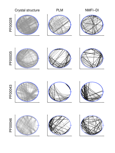
Figure 7: (Color online) Connections for four families overlaid on circles. Position ‘1’ is indicated by a dash. The leftmost column shows contacts in the crystal structure (dark gray for $d(i,j)<5$Å and light gray for 5Å$\leq d(i,j)<8.5$Å). The other two columns show the top $1.5N$ strongest ranked $|j-i|>4$-pairs for PLM and NMFI-DI, with gray for true positives and black for false positives.

Appendix B Other scores for naive mean-field inversion

We also investigated NMFI performance using the APC term for the $\mathcal{S}_{ij}^{DI}$ scoring and using our new $\mathcal{S}_{ij}^{CN}$ score. In the second case we first switch the parameter constraints from (9) to (8) using (26). Mean TP rates using the modified score are shown in Fig. 8. We observe that APC in $\mathcal{S}_{ij}^{DI}$ scoring increases TP rates slightly, while $\mathcal{S}_{ij}^{CN}$ scoring can improve TP rates overall. We remark, however, that for the second-highest ranked interaction ($p=2$) NMFI with the original $\mathcal{S}_{ij}^{DI}$ (NMFI-DI) ties with NMFI with $\mathcal{S}_{ij}^{CN}$ (NMFI-CN).

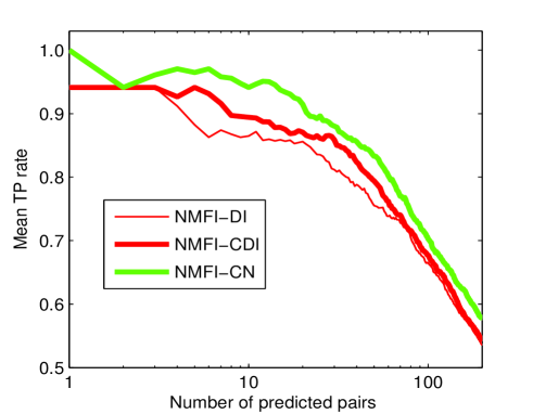
Figure 8: (Color online) Mean TP rates, using pairs with $|j-i|>4$, for NMFI with old score $\mathcal{S}_{ij}^{DI}$, new APC score $\mathcal{S}_{ij}^{CDI}$, and the norm score $\mathcal{S}_{ij}^{CN}$. Each curve corresponds to the best $\lambda$ for that particular score.

Motivated by the results of Fig. 8, we decided to compare NMFI and PLM under the $\mathcal{S}_{ij}^{CN}$ score. All figures in this paragraph show the best regularization for each method, unless otherwise stated. Figure 9 shows score vs. distance for all pairs in all families. Unlike Fig. 4, the two plots now show very similar profiles. We note, however, that NMFI’s $\mathcal{S}_{ij}^{CN}$ scores trend two to three times larger than PLM’s (the scales on the vertical axes are different). Perhaps this is an inherent feature of these methods, or simply a consequence of the different types of regularization.

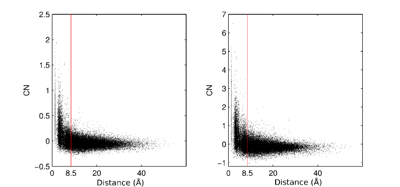
Figure 9: (Color online) Score plotted against distance for all position pairs in all 17 families for PLM (left) and NMFI-CN (right). The vertical line is our contact cutoff at 8.5Å.

Figure 10 shows the same situation as Fig. 3, but using $\mathcal{S}_{ij}^{CN}$ to score NMFI. The three best regularization choices for NMFI-CN turned out the same as before, i.e., $\lambda=1\cdot B_{eff}$, $\lambda=1.5\cdot B_{eff}$ and $\lambda=2.3\cdot B_{eff}$, but the best out of these three was now $\lambda=2.3\cdot B_{eff}$ (instead of $\lambda=1\cdot B_{eff}$). Comparing Fig. 3 and Fig. 10 one can see that the difference between the two methods is now smaller; for several families, the prediction quality is in fact about the same for both methods. Still, PLM maintains a somewhat higher TP rates overall.

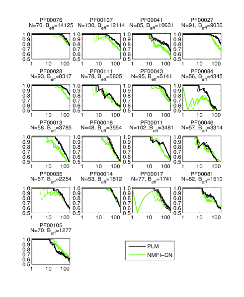
Figure 10: (Color online) Contact-detection results for all the families in our study (sorted by $B_{eff}$), now with the $\mathcal{S}_{ij}^{CN}$ score for NMFI. The y-axes are TP rates and the x-axes are the number of predicted contacts $p$, based on pairs with $|j-i|>4$. The three curves for each method are the three regularization levels yielding highest TP rates across all families. The thickened curve highlights the best one out of these three ($\lambda=2.3\cdot B_{eff}$ for NMFI-CN and $\lambda_{J}=0.01$ for PLM).

Figure 11 shows scatter plots for the same families as in Fig. 5 but using the $\mathcal{S}_{ij}^{CN}$ scoring for NMFI. The points now lie more clearly on a line, from which we conclude that the bends in Fig. 5 were likely a consequence of differing scores. Yet, the trends seen in Fig. 5 remain: NMFI gives more attention to neighbor pairs than does PLM.

In Fig. 12, we recreate the contact maps of Fig. 6 with NMFI-CN in place of NMFI-DI and find that the plots are more symmetric. As expected, asymmetry is seen primarily for small $|j-i|$; NMFI tends to crowd these regions with lots of loops.

To investigate why NMFI assembles so many top-scored pairs in certain neighbor regions, we performed an explicit check of the associated MSA columns. A relevant regularity was observed: when gaps appear in a sequence, they tend to do so in long strands. The picture can be illustrated by the following hypothetical MSA (in our implementation, the gap state is 1):

$$\begin{pmatrix}\cdots\\ \cdots$ 6 $5$ 9 $7$ 2 $6$ 8 $7$ 4 $4$ 2 $2\cdots\\ \cdots$ 1 $1$ 1 $1$ 1 $1$ 1 $1$ 1 $1$ 2 $8\cdots\\ \cdots$ 6 $5$ 2 $7$ 2 $3$ 8 $9$ 5 $4$ 2 $3\cdots\\ \cdots$ 3 $7$ 4 $7$ 2 $6$ 8 $7$ 9 $4$ 2 $3\cdots\\ \cdots$ 3 $7$ 4 $7$ 2 $3$ 8 $8$ 9 $4$ 2 $9\cdots\\ \cdots$ 1 $1$ 1 $1$ 1 $1$ 1 $4$ 5 $4$ 2 $9\cdots\\ \cdots$ 8 $5$ 9 $7$ 2 $9$ 8 $7$ 4 $4$ 2 $4\cdots\\ \cdots$ 1 $1$ 1 $1$ 1 $1$ 1 $1$ 1 $1$ 2 $4\cdots\\ \cdots\end{pmatrix}.$$

We recall that gaps (’1’ states) are necessary for satisfactory alignment of the sequences in a family and that in our procedure we treat gaps just another amino acid, with its associated interaction parameters. We then make the obvious observation that independent samples from a Potts model will only contain long subsequences of the same state with low probability. In other words, the model to which we fit the data cannot describe long stretches of ’1’ states, which is a feature of the data. It is hence quite conceivable that the two methods handle this discrepancy between data and models differently since we do expect this gap effect to generate large $J_{ij}(1,1)$ for at least some pairs with small $|j-i|$.

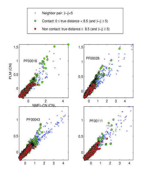
Figure 11: (Color online) Scatter plots of interaction scores for PLM and NMFI-CN from four families. For all plots, the axes are as indicated by the top left figure. The distance unit in the top box is Å.

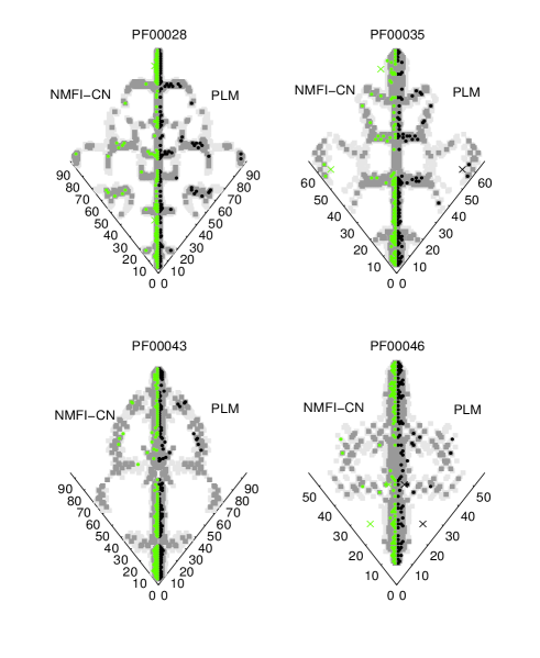
Figure 12: (Color online) Predicted contact maps for PLM (right part, black symbols) and NMFI-CN (left part, green symbols online) from four families. A pair $(i,j)$’s placement in the plots is found by matching positions $i$ and $j$ on the axes. Contacts are indicated by gray (dark for $d(i,j)<5$Å and light for 5Å$\leq d(i,j)<8.5$Å). True and false positives are represented by circles and crosses, respectively. Each figure shows the $1.5N$ strongest ranked pairs (including neighbors) for that family.

Figure 13 shows scatter plots for all coupling parameters $J_{ij}(k,l)$ in PF00014, which has a modest amount of gap sections, and in PF00043, which has relatively many. As outlines above, the $J_{ij}(1,1)$-parameters are among the largest in magnitude, especially for PF00043. We also note that the black dots steer to the right; NMFI clearly reacts more strongly to the gap-gap interactions than PLM.

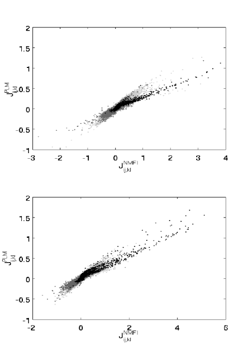
Figure 13: Scatter plots of estimated $J_{ij,kl}=J_{ij}(k,l)$ from PF00014 (top) and PF00043 (bottom). Black dots are ‘gap–gap’ interactions ($k=l=1$), dark gray dots are ‘gap–amino-acid’ interactions ($k=1$ and $l\neq 1$, or $k\neq 1$ and $l=1$), and light gray dots are ‘amino-acid–amino-acid’ interactions ($k\neq 1$ and $l\neq 1$).

Jones et al. journals/bioinformatics/JonesBCP12 disregarded contributions from gaps in their scoring by simply skipping the gap state when doing their norm summations. We tried this but found no significant improvement for either method. The change seemed to affect only pairs with small $|j-i|$ (which is reasonable), and our TP rates are based on pairs with $|j-i|>4$. If gap interactions are indeed responsible for reduced prediction qualities, removing their input during scoring is just a Band-Aid type solution. A better way would be to suppress them already in the parameter estimation step. That way, all interplay would have to be accounted for without them. Whether or not there are ways to effectively handle the inference problem in PSP by ignoring gaps or treating them differently, is an issue which goes beyond the scope of this work.

We also investigated whether the gap effect depends on the sequence similarity reweighting factor $x$, which up to here was chosen $x=0.9$. Perhaps the gap effect can be dampened by stricter definition of sequence uniqueness? In Fig. 14 we show another set of TP rates, but now for $x=0.75$. We also include results for NMFI run on alignment files from which all sequences with more than $20\%$ gaps have been removed. The best regularization choice for each method turned out the same as in Fig. 10: $\lambda=2.3\cdot B_{eff}$ for NMFI-CN and $\lambda_{J}=0.01$ for PLM. Overall, PLM maintains the same advantage over NMFI-CN it had in Fig. 10. Removing gappy sequences seems to trim down more TP rates than it raises, probably since useful information in the nongappy parts is discarded unnecessarily.

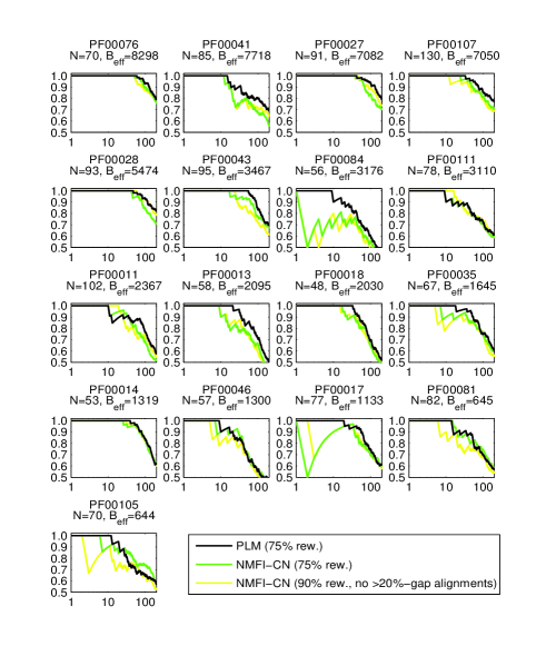
Figure 14: (Color online) Contact-detection results for all the families in our study. The y-axes are TP rates and x-axes are the number of predicted contacts $p$, based on pairs with $|j-i|>4$. Two curves are included for reweighting margin $x=0.75$, and one for reweighting margin $x=0.9$ after deletion of all sequences with more than $20\%$ gaps. Results for each method correspond to the regularization level yielding highest TP rates across all families ($\lambda=2.3\cdot B_{eff}$ for both NMFI-CN and $\lambda_{J}=0.01$ for PLM).

Appendix C Extension to 28 protein families

To sample a larger set of families, we conducted an additional survey of 28 families, now covering lengths across the wider range of 50-400. The list is given in Table 2. We here kept the reweighting level at $x=0.8$ as in pmid22106262 , while the TP rates were again calculated using the cutoff 8.5Å. The pseudocount strength for NMFI was varied in the same interval as in the main text. We did not try to optimize the PLM regularization parameters for this trial, but merely used $\lambda_{h}=\lambda_{J}=0.01$ as determined for the smaller families in the main text.

Figure 15 shows qualitatively the same behavior as in the smaller set of families: TP rates increase partly from changing from the $\mathcal{S}_{ij}^{DI}$ score to the $\mathcal{S}_{ij}^{CN}$ score, and partly from changing from NMFI to PLM. Our positive results thus do not seem to be particular to short-length families.

Apart from the average TP rate for each value of $p$ ($p$’th strongest predicted interactions) one can also evaluate performance by different criteria. In this larger survey we investigated the distribution of values of $p$ such that the TP rate in a family is one. Fig. 16 shows the histograms of the number of families for which the top $p$ predictions are correct, clearly showing that the difference between PLM and NMFI (using the two scores) primarily occurs at the high end. The difference in average performance between PLM and NMFI at least partially stems from PLM getting more strongest contact predictions with 100% accuracy.

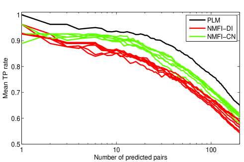
Figure 15: (Color online) Mean TP rates over the larger set of 28 families for PLM with $\lambda_{J}=0.01$ and varying regularization values for NMFI-CN and NMFI-DI.

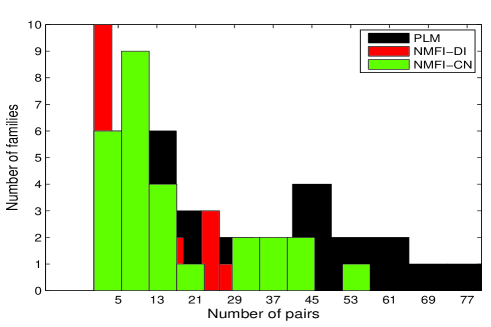
Figure 16: (Color online) Distribution of ’perfect’ accuracy for the three methods. The x-axis shows the number of top-ranked pairs for which the TP rates stays at one, and the y-axis shows the number of families.

ID	N	B	$B_{eff}(80\%)$	PDB ID	UniProt entry	UniProt residues
PF00006	215	10765	641	2r9v	ATPA_THEMA	149-365
PF00011	102	5024	2725	2bol	TSP36_TAESA	106-206
PF00014	53	2393	1478	5pti	BPT1_BOVIN	39-91
PF00017	77	2732	1312	1o47	SRC_HUMAN	151-233
PF00018	48	5073	335	2hda	YES_HUMAN	97-144
PF00025	175	2946	996	1fzq	ARL3_MOUSE	3-177
PF00026	314	3851	2075	3er5	CARP_CRYPA	105-419
PF00027	91	12129	7631	3fhi	KAP0_BOVIN	154-238
PF00028	93	12628	6323	2o72	CADH1_HUMAN	267-366
PF00032	102	14994	684	1zrt	CYB_RHOCA	282-404
PF00035	67	3093	1826	1o0w	RNC_THEMA	169-235
PF00041	85	15551	8691	1bqu	IL6RB_HUMAN	223-311
PF00043	95	6818	4052	6gsu	GSTM1_RAT	104-192
PF00044	151	6206	1422	1crw	G3P_PANVR	1-148
PF00046	57	7372	1761	2vi6	NANOG_MOUSE	97-153
PF00056	142	4185	1120	1a5z	LDH_THEMA	1-140
PF00059	108	5293	3258	1lit	REG1A_HUMAN	53-164
PF00071	161	10779	3793	5p21	RASH_HUMAN	5-165
PF00073	171	9524	487	2r06	POLG_HRV14	92-299
PF00076	70	21125	10113	1g2e	ELAV4_HUMAN	48-118
PF00081	82	3229	890	3bfr	SODM_YEAST	27-115
PF00084	56	5831	3453	1elv	C1S_HUMAN	359-421
PF00085	104	10569	6137	3gnj	VWF_HUMAN	1691-1863
PF00091	216	8656	917	2r75	FTSZ_AQUAE	9-181
PF00092	179	3936	1786	1atz	VWF_HUMAN	1691-1863
PF00105	70	2549	816	1gdc	GCR_RAT	438-507
PF00108	264	6839	2688	3goa	FADA_SALTY	1-254

Table 2: Domain families included in our extended study, listed with Pfam ID, length $N$, number of sequences $B$ (after removal of duplicate sequences), number of effective sequences $B_{eff}$ (under $x=0.8$, i.e., $80\%$ threshold for reweighting), and the PDB and UniProt specifications for the structure used to access the DCA prediction quality.

References

- (1) M. Weigt, R. White, H. Szurmant, J. Hoch, and T. Hwa, Proc. Natl. Acad. Sci. U. S. A. 106, 67 (2009)
- (2) F. Morcos, A. Pagnani, B. Lunt, A. Bertolino, D. S. Marks, C. Sander, R. Zecchina, J. N. Onuchic, T. Hwa, and M. Weigt, Proc. Natl. Acad. Sci. U. S. A. 108, E1293 (2011)
- (3) D. S. Marks, L. J. Colwell, R. P. Sheridan, T. A. Hopf, A. Pagnani, R. Zecchina, and C. Sander, PLoS One 6, e28766 (2011)
- (4) J. Sulkowska, F. Morcos, M. Weigt, T. Hwa, and J. Onuchic, Proc. Natl. Acad. Sci. U. S. A. 109, 10340 (2012)
- (5) T. Nugent and D. T. Jones, Proc. Natl. Acad. Sci. U. S. A. 109, E1540 (2012)
- (6) M. Punta, P. C. Coggill, R. Y. Eberhardt, J. Mistry, J. G. Tate, C. Boursnell, N. Pang, K. Forslund, G. Ceric, J. Clements, A. Heger, L. Holm, E. L. L. Sonnhammer, S. R. Eddy, A. Bateman, and R. D. Finn, Nucleic Acids Res. 40, D290 (2012)
- (7) L. Burger and E. van Nimwegen, PLoS Comput. Biol. 6, E1000633 (2010)
- (8) S. Balakrishnan, H. Kamisetty, J. Carbonell, S. Lee, and C. Langmead, Proteins: Struct., Funct., Bioinf. 79, 1061 (2011)
- (9) D. T. Jones, D. W. A. Buchan, D. Cozzetto, and M. Pontil, Bioinformatics 28, 184 (2012)
- (10) H. J. Kappen and F. B. Rodriguez, in Advances in Neural Information Processing Systems (The MIT Press, 1998) pp. 280–286
- (11) E. Schneidman, M. Berry, R. Segev, and W. Bialek, Nature 440, 1007 (2006)
- (12) A. Braunstein and R. Zecchina, Phys. Rev. Lett. 96, 030201 (2006)
- (13) A. Braunstein, A. Pagnani, M. Weigt, and R. Zecchina, J. Stat. Mech. 2008, P12001 (2008)
- (14) Y. Roudi, J. A. Hertz, and E. Aurell, Front. Comput. Neurosci. 3 (2009), doi:“bibinfo–doi˝%**** ̵article-v12-dec18.bbl ̵Line ̵250 ̵****–10.3389/neuro.10.022.2009˝
- (15) S. Cocco, S. Leibler, and R. Monasson, Proc. Natl. Acad. Sci. U. S. A. 106, 14058 (2009)
- (16) V. Sessak and R. Monasson, J. Phys. A: Math. Theor. 42, 055001 (2009)
- (17) M. Mézard and T. Mora, J. Physiol. (Paris) 103, 107 (2009)
- (18) E. Marinari and V. V. Kerrebroeck, J. Stat. Mech.(2010), doi:“bibinfo–doi˝–10.1088/1742-5468/2010/02/P02008˝
- (19) S. Cocco and R. Monasson, Phys. Rev. Lett. 106, 090601 (2011)
- (20) F. Ricci-Tersenghi, J. Stat. Mech.(2012)
- (21) H. Nguyen and J. Berg, J. Stat. Mech.(2012)
- (22) H. Nguyen and J. Berg, Phys. Rev. Lett. 109 (2012)
- (23) E. Aurell and M. Ekeberg, Phys. Rev. Lett. 108, 090201 (2012)
- (24) A. Hyvärinen, J. Karhunen, and E. Oja, Independent Component Analysis, Adaptive and Learning Systems for Signal Processing, Communications, and Control (John Wiley & Sons, 2001)
- (25) J. Rissanen, Information and Complexity in Statistical Modeling (Springer, 2007)
- (26) M. J. Wainwright and M. I. Jordan, Foundations and Trends in Machine Learning 1, 1 (2008)
- (27) P. Ravikumar, M. J. Wainwright, and J. D. Lafferty, Ann. Stat. 38, 1287 (2010)
- (28) H. Ackley, E. Hinton, and J. Sejnowski, Cogn. Sci. 9, 147 (1985)
- (29) G. Parisi, Statistical Field Theory (Addison Wesley, 1988)
- (30) L. Peliti, Statistical Mechanics in a Nutshell (Princeton University Press, 2011) ISBN ISBN-13: 9780691145297
- (31) K. Fischer and J. Hertz, Spin Glasses (Cambridge University Press, 1993) ISBN 0521447771, 9780521447775
- (32) I. Pagani, K. Liolios, J. Jansson, I. Chen, T. Smirnova, B. Nosrat, and M. V.M., Nucleic Acids Res. 40, D571 (2012)
- (33) The Uniprot Consortium, Nucleic Acids Res. 40, D71 (2012)
- (34) H. Berman, G. Kleywegt, H. Nakamura, and J. Markley, Structure 20, 391 (2012)
- (35) U. Göbel, C. Sander, R. Schneider, and A. Valencia, Proteins: Struct., Funct., Genet. 18, 309 (1994)
- (36) S. W. Lockless and R. Ranganathan, Science 286, 295 (1999)
- (37) A. A. Fodor and R. W. Aldrich, Proteins: Struct., Funct., Bioinf. 56, 211 (2004)
- (38) A. S. Lapedes, B. G. Giraud, L. Liu, and G. D. Stormo, Lecture Notes-Monograph Series: Statistics in Molecular Biology and Genetics 33, 236 (1999)
- (39) J. Besag, The Statistician 24, 179–195 (1975)
- (40) A. Schug, M. Weigt, J. Onuchic, T. Hwa, and H. Szurmant, Proc. Natl. Acad. Sci. U. S. A. 106, 22124 (2009)
- (41) A. E. Dago, A. Schug, A. Procaccini, J. A. Hoch, M. Weigt, , and H. Szurmant, Proc. Natl. Acad. Sci. U. S. A. 109, 10148 (2012)
- (42) T. A. Hopf, L. J. Colwell, R. Sheridan, B. Rost, C. Sander, and D. S. Marks, Cell 149, 1607 (2012)
- (43) E. T. Jaynes, Physical Review Series II 106, 620–630 (1957)
- (44) E. T. Jaynes, Physical Review Series II 108, 171–190 (1957)
- (45) G. Darmois, C.R. Acad. Sci. Paris 200, 1265–1266 (1935), in French
- (46) E. Pitman and J. Wishart, Math. Proc. Cambridge Philos. Soc. 32, 567–579 (1936)
- (47) B. Koopman, Trans. Am. Math. Soc. 39, 399–409 (1936)
- (48) A. Kholodenko, J. Stat. Phys. 58, 357 (1990)
- (49) T. Tanaka, Neural Comput. 12, 1951–1968 (2000)
- (50) S. ichi Amari, S. Ikeda, and H. Shimokawa, “Information geometry and mean field approximation: the alpha-projection approach,” in Advanced Mean Field Methods – Theory and Practice (MIT Press, 2001) Chap. 16, pp. 241–257, ISBN 0-262-15054-9
- (51) S. D. Dunn, L. M. Wahl, and G. B. Gloor, Bioinformatics 24, 333 (2008)
- (52) G. Hinton, Neural Comput. 14, 1771–1800 (2002)
- (53) M. Gutmann and A. Hyvärinen, J. Mach. Learn. Res. 13, 307 (2012)