Full spectral fitting of Milky Way and M31 globular clusters: ages and metallicities

Abstract

Context. The formation and evolution of disk galaxies are long standing questions in Astronomy. Understanding the properties of globular cluster systems can lead to important insights on the evolution of its host galaxy.

Aims. We aim to obtain the stellar population parameters – age and metallicity – of a sample of M31 and Galactic globular clusters. Studying their globular cluster systems is an important step towards understanding their formation and evolution in a complete way.

Methods. Our analysis employs a modern pixel-to-pixel spectral fitting technique to fit observed integrated spectra to updated stellar population models. By comparing observations to models we obtain the ages and metallicities of their stellar populations. We apply this technique to a sample of 38 globular clusters in M31 and to 41 Galactic globular clusters, used as a control sample.

Results. Our sample of M31 globular clusters spans ages from 150 Myr to the age of the Universe. Metallicities [Fe/H] range from –2.2 dex to the solar value. The age-metallicity relation obtained can be described as having two components: an old population with a flat age-[Fe/H] relation, possibly associated with the halo and/or bulge, and a second one with a roughly linear relation between age and metallicity, higher metallicities corresponding to younger ages, possibly associated with the M31 disk. While we recover the very well known Galactic GC metallicity bimodality, our own analysis of M31’s metallicity distribution function (MDF) suggests that both GC systems cover basically the same [Fe/H] range yet M31’s MDF is not clearly bimodal. These results suggest that both galaxies experienced different star formation and accretion histories.

1 Introduction

Globular clusters (GCs) are widely considered as excellent astrophysical laboratories. Their age and metallicities, in particular, trace the main (astro)physical processes responsible for the formation and evolution of their host galaxies. However, differently from the Milky Way, most of the extragalactic GCs cannot be resolved into individual stars.

The techniques to estimate ages and metallicities of extragalactic GCs have classically fallen into two broad categories. Those relying on photometry (e.g. Fan et al., 2006) are more susceptible to the age-metallicity degeneracy in the sense that young metal-rich populations are photometrically indistinguishable from older metal-poor populations (but see, e.g., Ma et al., 2007). The different spectroscopic methods, however, are inspired by the Lick/IDS system of absorption line indices (e.g. Worthey et al., 1994, and references therein) — from linear metallicity calibrations (e.g. Brodie & Huchra, 1990) to those which perform the simultaneous $\chi$²-minimisation of a large number of spectral indices (see, e.g., Proctor et al., 2004). Nevertheless, both photometric and spectroscopic methods are dependent on the accurate modelling of simple stellar populations (SSPs, see, e.g., Bruzual & Charlot, 2003; Le Borgne et al., 2004; Delgado et al., 2005; Maraston, 2005; Coelho et al., 2007; Percival et al., 2009; Lee et al., 2009; Conroy & Gunn, 2010; Vazdekis et al., 2010).

More recently, it is becoming increasingly common to use spectral fitting on a pixel-to-pixel basis to study integrated spectra of stellar clusters (e.g. Dias et al., 2010). This technique is an improvement over older methods and has been recently discussed in e.g. Koleva et al. (2008); Cid Fernandes & González Delgado (2010) and references therein. This method has advantages such as making use of all the information available in a spectrum (making it possible to perform analysis at lower S/N) and not being limited by the physical broadening, since the internal kinematics is determined simultaneously with the population parameters. In some of its flavours, this method is also insensitive to extinction or flux calibrating errors. It has also been shown that full spectrum fitting reproduces better the results from colour-magnitude diagrams (CMDs) than other methods (e.g. Wolf et al., 2007).

In this study, we have used the spectrum fitting code ULySS (Koleva et al., 2009) to compare, on a pixel-by-pixel basis, the integrated spectrum of 38 spectra of GCs in M31 to simple stellar population models in order to derive their ages and metallicities. Our sample comprises 35 integrated spectra previously analysed by Beasley et al. (2004), and three outer halo clusters taken from Alves-Brito et al. (2009). In addition, we have also analysed integrated spectra of 41 Galactic GCs presented in Schiavon et al. (2005), whose populations have been studied with CMDs and spectroscopy of individual stars. Both, Galactic and M31 GCs were analysed in the same way. The Galactic sample acts as a control sample to estimate the reliability of the fitting method.

Our nearest ($\sim$780 kpc, Holland, 1998) giant spiral galaxy M31 is a natural target to test the current ideas about the formation and evolution of galaxies in the Local Universe. As pointed out in Alves-Brito et al. (2009), a remarkable difference between the M31 and the Galactic GC system is that M31 hosts more GCs (by a factor of 2–3) than the Milky Way. Furthermore, there have been suggestions that M31 may have a significant population of young and intermediate age (less than 8 Gyr) that is not found in the Galactic system. The metallicity distribution function (MDF) of M31 (through both giant stars and GCs) and other galaxies (see, e.g. Alves-Brito et al., 2011; Usher et al., 2012) has been a controversial topic regarding its shape and distribution when compared with our own Galaxy. In particular, the presence (or not) of colour-[Fe/H] bimodality is one of the interesting and intriguing open questions in the field. Therefore, these (dis)similarities between the different spiral galaxies in the Local Group need to be investigated through different techniques to better understand the different process(es) in which spiral galaxies are formed and have evolved in the Universe.

The paper is organised as follows. In Sect. 2 we describe our sample. In Sect. 3 we present the stellar population analysis. In Sect. 4 we discuss the results obtained. Concluding remarks are given in Sect. 5.

2 Sample

2.1 M31 GCs

The integrated spectra used in this study were previously studied by Alves-Brito et al. (2009) and Beasley et al. (2004). The former provided spectra for three outer halo GCs at projected distances beyond $\approx$ 80 kpc from M31. These spectra were observed with the cross-dispersed, high-resolution spectrograph HIRES instrument on the Keck 1 telescope, covering a broad wavelength range of $\lambda\lambda=4020$–$8520$ Å, at a spectral resolving power of $R\approx 50,000$. Spectroscopic age and metallicities were obtained by using metallicity calibrations from Mgb, CH and Mg2 indices. In addition, the authors also employed the simultaneous $\chi$²-minimisation of a large number of spectral indices, approach introduced by Proctor et al. (2004).

The second source of data is detailed in Beasley et al. (2004), who made a analysis of high-quality integrated spectral indices in M31. We have only used the spectra obtained with the Low Resolution Imaging Spectrograph mounted on the Keck I telescope, covering a spectral range of $\lambda\lambda=3670$–$6200$ Å and with a full width at half-maximum (FWHM) resolution of 5 Å. The sample chemical properties were studied through the measurement of Lick line strengths.

In Table 1 we list the M31 GCs analysed in the present work, and we refer the reader to Alves-Brito et al. (2009) and Beasley et al. (2004) for additional information about the observations and data reduction. The projected distances shown in Table 1 were calculated relative to an adopted M31 central position of $\alpha_{\rm J2000}$ = 00^h42^m44^s.30, $\delta_{\rm J2000}$ = +41^o16^′09.90$\aas@@fstack{\prime\prime}$4. In addition, a position angle for the X-coordinate of 38^o (Kent et al., 1989) as well as a distance of 780 kpc (Holland, 1998) were adopted. At this distance, 1 arc-min corresponds to 228 pc.

Table 1: M31 GCs analysed in the present work.

ID	R.A. (J2000.0)	Decl. (J2000.0)	dp	S/N	Reference
			(kpc)	(pixel-1)
B126	00:42:43.481	+41:12:42.47	0.79	73	a
B134	00:42:51.678	+41:44:03.42	0.52	70	a
B158	00:43:14.406	+41:47:21.28	2.40	120	a
B163	00:43:17.640	+41:27:44.91	3.01	170	a
B222	00:44:25.380	+41:14:11.62	4.37	30	a
B225	00:44:29.560	+41:21:35.27	4.69	169	a
B234	00:44:46.375	+41:29:17.77	6.03	71	a
B292	00:36:16.666	+40:58:26.58	17.15	32	a
B301	00:38:21.581	+40:03:37.16	20.09	31	a
B302	00:38:33.500	+41:20:52.29	10.81	28	a
B304	00:38:56.940	+41:10:28.41	9.85	34	a
B305	00:38:58.922	+40:16:31.78	16.74	15	a
B307	00:39:18.477	+40:32:58.05	13.27	20	a
B310	00:39:25.752	+41:23:33.14	8.67	35	a
B313	00:39:44.599	+40:52:55.05	9.38	52	a
B314	00:39:44.599	+40:14:07.95	16.15	17	a
B316	00:39:53.604	+40:41:39.29	10.78	20	a
B321	00:40:15.545	+40:27:46.50	12.78	30	a
B322	00:40:17.270	+40:39:04.70	10.57	69	a
B324	00:40:20.477	+41:40:49.38	8.33	71	a
B327	00:40:24.107	+40:36:22.52	10.91	30	a
B328	00:40:24.529	+41:40:23.15	8.13	30	a
B331	00:40:26.642	+41:42:04.28	8.35	15	a
B337	00:40:48.477	+42:12:11.06	13.71	178	a
B347	00:42:22.892	+41:24:27.58	8.79	61	a
B350	00:42:28.442	+40:24:51.12	11.73	39	a
B354	00:42:47.645	+42:00:24.73	10.10	30	a
B365	00:44:36.445	+42:17:20.57	14.77	60	a
B380	00:46:06.238	+42:00:53.13	13.36	43	a
B383	00:46:11.498	+41:19:41.48	8.94	85	a
B393	00:47:01.204	+41:24:66.39	11.16	43	a
B398	00:47:57.786	+41:48:45.66	15.32	44	a
B401	00:48:08.508	+41:40:41.93	14.96	54	a
MGC1	00:50:42.459	+32:54:58.78	116.05	20	b
MCGC5	00:35:59.700	+35:11:03.60	78.49	20	b
MCGC10	01:07:26.318	+35:46:48.41	99.85	20	b
NB16	00:42:33.094	+41:20:16.41	1.05	142	a
NB89	00:42:44.780	+41:14:44.20	0.34	110	a

Notes.— The first column gives the GC identification, as in the Bologna catalogue (Galleti et al., 2004). Second and third columns give the coordinates of the objects, in J2000. Fourth column shows the projected distance of the cluster to the centre of M31 (see text in §2.1). Fifth column shows the S/N of the spectra as given in the corresponding paper; when this information was not available (clusters B302, B305, B307, B316, B331, B354), we estimated the S/N around 5000 Å using standard IRAF routines. Sixth column gives the reference of the spectra: (a) for Beasley et al. (2004) and (b) for Alves-Brito et al. (2009).

2.2 Galactic GCs

The sample of Galactic GCs spectra is given in Table LABEL:tab_res_mw, whose observations were taken from Schiavon et al. (2005). The observations were performed with a long-slit spectrograph in drift-scan mode in order to integrate the population within one core radius. The spectra cover the range $\lambda\lambda$ = 3350 – 6430 $\AA$ at a resolution of about FWHM = 3 $\AA$. The mean S/N varies from 50 to 240 $\AA^{-1}$ depending on the wavelength. We refer the reader to Schiavon et al. (2005) for more details on the observations and data reduction.

The aim of analysing this Galactic sample is twofold: first, we use it as a control sample where we can evaluate the performance of the fitting technique by comparing our results to studies of CMD and spectroscopy of individual stars; and second, by ensuring that the same analysis is applied consistently to the M31 and Galactic sample, the latter acts as a reference system to which the M31 GC system is compared.

We searched the literature for good independent determinations of ages and metallicities of this sample. Fitting theoretical isochrones to GC CMDs is generally accepted as the most secure age determination possible when using photometry; however, the results do vary between sets of isochrones and methods of analysis, and the absolute derived age depends on model zero points, input physics, colour-T_eff transformation, distance uncertainties and foreground reddening (e.g. Chaboyer et al., 1998; Buonanno et al., 1998; Meissner & Weiss, 2006). In this work we relied on the relative ages derived homogeneously for a large sample of clusters from De Angeli et al. (2005) and Marín-Franch et al. (2009). Those relative ages were converted to absolute ages by adopting a conservative value of 13 $\pm$ 2.5 Gyr for 47 Tucanae (Zoccali et al., 2001). We additionally added values for NGC 6528 and NGC 6553 from Momany et al. (2003) and Beaulieu et al. (2001), respectively.

Regarding the metallicities, we adopt two homogeneous compilations found in literature: the compilation by Carretta et al. (2009), who analysed high resolution stellar spectra in 19 globular clusters, and brought the lower resolution measurements from Zinn & West (1984); Kraft & Ivans (2003); Rutledge et al. (1997) to a common metallicity-scale; and the compilation by Schiavon et al. (2005), based on measurements from Kraft & Ivans (2003); Carretta & Gratton (1997).

3 Analysis

We obtained ages and metallicities for the GCs through the comparison of their integrated spectra to SSP models, using the public code ULySS (Koleva et al., 2009), described briefly below.

ULySS is a software package performing spectral fitting in two astrophysical contexts: the determination of stellar atmospheric parameters and the study of the star formation and chemical enrichment history of galaxies. In ULySS, an observed spectrum is fitted against a model (expressed as a linear combination of components) through a non-linear least-squares minimisation. In the case of our study, the components are SSP models.

We adopt SSP models by Vazdekis et al. (2010), which cover the wavelength range 3540 – 7400Å  at a resolution of FWHM $\sim$ 2.5Å. Ages range between 63 Myr and 18 Gyr, and metallicities [Fe/H] between –2.32 and +0.22 dex. These models are based on MILES stellar library (Sánchez-Blázquez et al., 2006; Cenarro et al., 2007) and Girardi et al. (2000) evolutionary tracks. Being based on an empirical library, the models follow the abundance pattern of the solar neighbourhood, namely they are solar-scaled around solar metallicities, and $\alpha$-enhanced for low metallicities (Milone et al., 2011).

ULySS matches model and observation continua through a multiplicative polynomial, determined during the fitting process. Therefore, ULySS is not sensitive to flux calibration, galactic extinction, or any other cause affecting the shape of the spectrum. We run ULySS with its global minimisation option, i.e., each fitting was performed starting from several guesses; this is an important feature that minimises the risks of results being biased by local minima.

For each spectrum we run 300 Monte Carlo (MC) simulations. The simulations consist of analyses of the spectrum with a random noise added, according to the S/N of the observation. As explained in Koleva et al. (2009), the MC simulations take into account the correlation between pixels and thus reproduce the correct noise spectrum, giving a robust estimate of the errors. We adopt the final stellar populations parameters to be the mean values of the 300 simulations, and our final uncertainties are the 1 $\sigma$ value of the simulations results. We quote a minimum error of 10% in age to account for possible systematic errors in the isochrones used in the SSP models (e.g. Gallart et al., 2005), when the 1 $\sigma$ value is smaller than this limit.

A possible disadvantage of spectral fitting, compared to Lick indices, is that the method may in principle be sensitive to the wavelength range fitted. Reports on this effect in literature are contradictory: Koleva et al. (2008) has concluded that the sensitivity to the wavelength range is not critical; at odds with this conclusion, Walcher et al. (2009) reports that while fitting globular clusters of the Galactic bulge, the results are more accurate when the fitting is limited to a wavelength range $\sim$ 530 Å wide centred at 5100 Å.

We thus performed some tests on the dependence with the wavelength window by fitting the Galactic GCs sample at different wavelength ranges. The widest range we tested was 3650 – 6150 Å (the total range covered by Beasley et al. 2004 observations) and the shortest 4828 – 5364 Å (favoured by Walcher et al. 2009). We also tested the wavelength used in Koleva et al. (2008, 4000 – 5700 Å) and the range 4000 – 5400 Å, similar to the coverage of Alves-Brito et al. (2009) observations.

4 Results

4.1 Stellar populations in the Galaxy — verifying the method

By analysing the Galactic sample at different wavelength windows, we verified that the wavelength choice has little influence on the metallicities derived via spectral fitting. On the other hand, the ages may change in a non-negligible way: in particular, fitting the widest range resulted in nearly a third of the GCs being fitted with intermediate ages (down to 4 Gyr). Possible sources of errors are: blue horizontal branches or blue stragglers not properly taken into account on the models, which is known to affect spectroscopic ages both in spectral fitting and Lick indices (e.g. de Freitas Pacheco & Barbuy, 1995; Koleva et al., 2008), deficiencies in the observations (diffuse light affecting the blue region and poor subtraction of telluric lines affecting the red, as mentioned in Koleva et al. 2008) and limitations in the SSP models (chemical patterns different than the ones in MILES library).

In the present work we favour the wavelength range 4000 – 5400Å which, among the wavelength windows we tested, is the one which best reproduced the CMD ages of the Galactic globular clusters. The results of this fitting run are shown in Table LABEL:tab_res_mw together with literature values. Comparisons between our results and literature are also shown in Figures 1 and 2 for ages and metallicities, respectively. Several of the Galactic GCs have multiple observations and we fitted each spectrum individually.

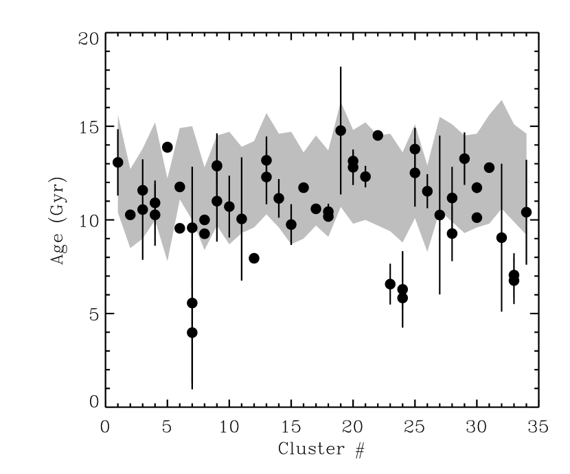
Figure 1: Comparison between the ages derived via spectral fitting (filled circles) and ages derived via CMD (filled grey pattern) for our sample of Galactic GCs. The number in the $x$-axis identifies the GCs (1: NGC 104; 2: NGC 1851; 3: NGC 1904; 4: NGC 2298; 5: NGC 2808; 6: NGC 3201; 7: NGC 5286; 8: NGC 5904; 9: NGC 5927; 10: NGC 5946; 11: NGC 5986; 12: NGC 6121; 13: NGC 6171; 14: NGC 6218; 15: NGC 6235; 16: NGC 6254; 17: NGC 6266; 18: NGC 6284; 19: NGC 6304; 20: NGC 6342; 21: NGC 6352; 22: NGC 6362; 23: NGC 6388; 24: NGC 6441; 25: NGC 6528; 26: NGC 6544; 27: NGC 6553; 28: NGC 6624; 29: NGC 6637; 30: NGC 6652; 31: NGC 6723; 32: NGC 6752; 33: NGC 7078; 34: NGC 7089).

In Fig. 1 it can be seen that six clusters have spectroscopic ages which are outside the range of allowed CMD values: NGC 2808 (GC #5 in Fig. 1), NGC 5286 (GC #7), NGC 6121 (GC #12), NGC 6388 (GC #23), NGC 6441 (GC #24), NGC 7078 (GC #33).

In the case of NGC 5286 (GC #7), it is striking that three observations of the same cluster resulted in ages different by almost 6 Gyr. According to the observation log in Schiavon et al. (2005), the three observations of this GC were taken at different slit positions or extraction aperture. A visual inspection of the fitting showed that in two exposures the observed Balmer lines are visibly narrower than the model, even though the metallic lines are well fitted (this pattern is also present in NGC 6752, GC # 32). We suspect that contamination from foreground stars hampered the observations. A visual inspection of the field around this GC in Aladin shows a handful of bright foreground stars close to the cluster. Given that the observations were performed in drift-scan mode, diffuse light from one of these stars might explain the failure of fitting the line profiles. For the remaining clusters, there was no obvious pattern in the visual inspection of the fitting, so we further investigated other sources of problems that could impact the derived ages.

It is well established in literature (e.g. Gratton et al., 2012) that virtually all clusters harbour populations with anti-correlated C–N, O–Na (and sometimes Mg–Al) abundances. In this sense, a comparison to strict SSP models might not be adequate in many cases. In Coelho et al. (2011, 2012) the authors investigate, by means of stellar population modelling, the effect of populations with CNONa variations in spectral indices and integrated spectra. Inside the wavelength range fitted in this work, we obtain from Fig. 5 in Coelho et al. (2012) that the range $\sim$4150–4220Å is affected by CNONa anti-correlated abundances. We investigated if these chemical variations could explain the age mismatch by repeating the fitting of the clusters NGC 2808, NGC 6121, NGC 6388, NGC 6441, NGC 7078, masking the CNONa affected region. We verified that the masking does not improve the age results, the differences between masking or not the CNONa region being $\Delta$age = 0.1 $\pm$ 0.2 Gyr. We conclude therefore that CNONa anti-correlations in the integrated spectra of clusters cannot explain the cases where spectroscopic ages do not match the CMD values.

The test above does not guarantee against the effect of multiple main sequences and/or sub-giant branches, clusters for which remarkably a single age isochrone is not adequate to fit the CMD. This is the case of NGC 2808 (Piotto et al., 2007), which is known to harbour three main sequences and a very complex horizontal branch. In such striking cases, it is not disquieting that comparing the observations to SSP models would fail.

Except for NGC 2808, the other clusters with deviating spectroscopic ages are all younger than the CMD ages by at least 2–3 Gyr. Our initial interpretation was the potential presence of HB morphologies which are not well represented in the SSP models. Extended HB morphologies are long known in literature to bias spectroscopic ages towards lower values (e.g. de Freitas Pacheco & Barbuy, 1995; Lee et al., 2000; Schiavon et al., 2004; Mendel et al., 2007; Ocvirk, 2010). Koleva et al. (2008) manages to reconcile some of the spectroscopic ages of galactic clusters with CMD measurements when a hot star component is added to the fitting, to mimic the presence of blue horizontal branch stars or blue stragglers. It is not straightforward, however, to predict how the HB morphology will impact the spectroscopic ages. The effective impact of the HB morphology on spectroscopic age is likely a non-trivial interplay between the wavelength range fitted (in the sense that bluer regions will be more sensitive to hotter HB stars) and the exact morphology (or lack of) predicted by the underlying isochrone of the stellar population model, this morphology also being dependent on the age and metallicity of the modelled population.

Using the study by Gratton et al. (2010) on the galactic clusters HB morphologies, we searched for patterns of the HB morphologies that could correlate with the clusters with deviant ages, but could not find any. The only note of interest is that four of these clusters (NGC2808, NGC6388, NGC6441, NGC7078) have high values of R’ (larger than 0.8). Nevertheless, cluster NGC 5927 (GC #9) also has a very high R’ and its spectroscopic age matches the CMD range.

Regarding the metallicities derived via spectral fitting, in Fig. 2 we compare our [Fe/H] values with those compiled by Carretta et al. (2009) (black triangles) and Schiavon et al. (2005) (blue squares). The overall difference (this work $-$ Schiavon et al.) is of –0.05 $\pm$ 0.16 dex, while (this work $-$ Carretta et al.) is –0.15 $\pm$ 0.17 dex. Even though the agreement with Schiavon et al. scale is better on average, it was pointed out by the referee that there seems to be a slope between our results and Schiavon et al. scale (the relation crossing the line of equality). On the other hand, the offset between our results and Carretta et al. scale is nearly constant, thus the differences between our results and this scale might be explained by a zero-point offset.

The scatter we obtain between our metallicities and the stellar analysis is compatible with the difference between Schiavon et al. and Carretta et al. scales (0.10 $\pm$ 0.20 dex), which are both based on high resolution stellar spectroscopy. It is a remarkable agreement between metallicities from integrated light at medium spectral resolutions and high-resolution stellar analysis.

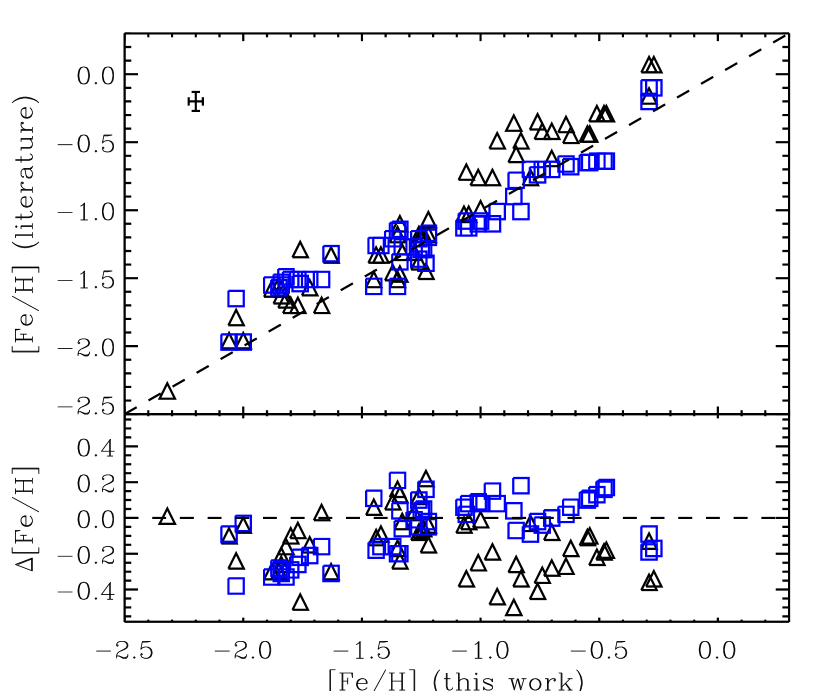
Figure 2: Top panel: Comparison of metallicities obtained with the spectral fitting (this work) versus the values compiled in literature by Schiavon et al. (2005) (blue squares) and Carretta et al. (2009) (black triangles) for the Galactic GCs. The error bar in the top left corner indicates the mean error values. Bottom panel: [Fe/H] residuals (ours minus literature values).

From the analysis of the galactic sample we conclude that regarding the age determination, the method returned accurate results except for six clusters: NGC 2808, NGC 5286, NGC 6121, NGC 6388, NGC 6441, NGC 7078. In the case of NGC 5286 (and possibly NGC 6752, whose spectroscopic age marginally matches the CMD range), we suspect that contamination from foreground stars hampered the observations. NGC 2808 is a striking case of a cluster with triple main sequences, and a failure when comparing to SSP models is not disquieting. For the remaining four clusters, or $\sim$12% of our galactic sample, ages are underestimated by $\sim$2–3 Gyr and we cannot provide a robust explanation for these differences. We confirmed that the presence of populations with CNONa anti-correlated abundances cannot explain the age differences. If this age difference is related to HB morphologies, as usually claimed in literature, its exact effect remains to be better understood, given that not all GC with extended HB were affected. We reproduced the CMD ages of other GCs known to have blue components (such as NGC 5946 and NGC 6284), without invoking additional parameters in the fitting (such as a free amount of hot stars in Koleva et al. 2008). The mean difference (this work - literature) is of –0.8 Gyr with an r.m.s. of 1.7 Gyr, for the sub-sample with fitted ages inside the observational uncertainties; and –1.8 Gyr with a r.m.s. of 2.8 Gyr for the whole sample.

As for the metallicities, the method gives results in accordance with determinations from high resolution stellar spectroscopy (R 30,000), with a r.m.s. of the same order of the r.m.s. between two different sets of high-resolution results as presented in the previous paragraph.

4.2 Stellar populations in M31 GCs

We analysed the M31 sample with the same set up and procedure as in the galactic sample, and our derived ages and metallicities are presented in Table 3. We show in Fig. 3 the fitting of two spectra in our M31 sample, for illustration purposes. We obtain a large range of ages, from $\sim$150 Myr (B322) to very old ages. In fact, three of the objects (B163, B393, and B398) were given “older than the Universe” ages (13.75 $\pm$ 0.11 Gyr; Jarosik et al., 2011). In these cases, $\chi^{2}$ maps of age distributions show a valley of low values starting around $\sim$ 6 Gyr and almost flat with metallicity, indicating that the results are degenerate in age. The metallicities in our sample range from –2.2 dex to +0.1 dex.

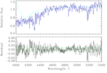
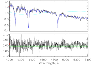
Figure 3: Spectral fitting of the GCs B163 (left-hand panel) and B380 (right-hand panel). The top panels show the spectra in black and the best fit in blue. The cyan lines are the multiplicative polynomials. The bottom panels are the residuals from the best fit, where the continuous green lines mark the 1-$\sigma$ deviation as expected by the input S/N, and the dashed green lines mark the zero y-axis. This plot is best seen in colour (online version only).

Table 3: Ages and metallicities for M31 GCs derived in this work.

Cluster	Age (Gyr)	[Fe/H]
B126	2.41 $\pm$ 0.86	-1.19 $\pm$ 0.15
B134	13.72 $\pm$ 2.70	-0.89 $\pm$ 0.04
B158	12.44 $\pm$ 1.24	-0.74 $\pm$ 0.02
B163	16.86 $\pm$ 0.43	-0.29 $\pm$ 0.01
B222	1.16 $\pm$ 0.12	-0.28 $\pm$ 0.03
B225	11.38 $\pm$ 1.74	-0.44 $\pm$ 0.03
B234	10.87 $\pm$ 1.10	-0.73 $\pm$ 0.02
B292	4.09 $\pm$ 0.47	-1.54 $\pm$ 0.04
B301	15.89 $\pm$ 4.97	-1.19 $\pm$ 0.12
B302	11.23 $\pm$ 1.12	-1.49 $\pm$ 0.05
B304	8.53 $\pm$ 2.22	-1.27 $\pm$ 0.06
B305	0.98 $\pm$ 0.10	0.07 $\pm$ 0.02
B307	1.68 $\pm$ 0.17	0.02 $\pm$ 0.02
B310	5.56 $\pm$ 0.66	-1.49 $\pm$ 0.05
B313	12.67 $\pm$ 1.27	-0.83 $\pm$ 0.02
B314	0.79 $\pm$ 0.08	-0.12 $\pm$ 0.02
B316	1.46 $\pm$ 0.26	-0.00 $\pm$ 0.13
B321	0.20 $\pm$ 0.02	-0.07 $\pm$ 0.06
B322	0.14 $\pm$ 0.09	-0.32 $\pm$ 0.31
B324	1.00 $\pm$ 0.10	-0.13 $\pm$ 0.09
B327	0.90 $\pm$ 0.54	-1.56 $\pm$ 0.09
B328	2.58 $\pm$ 0.81	-1.60 $\pm$ 0.05
B331	5.97 $\pm$ 1.34	-0.64 $\pm$ 0.07
B337	1.91 $\pm$ 0.98	-0.58 $\pm$ 0.32
B347	8.06 $\pm$ 1.29	-2.05 $\pm$ 0.04
B350	8.70 $\pm$ 1.39	-1.66 $\pm$ 0.04
B354	11.43 $\pm$ 1.14	-2.01 $\pm$ 0.03
B365	9.01 $\pm$ 1.73	-1.34 $\pm$ 0.04
B380	0.58 $\pm$ 0.06	-0.06 $\pm$ 0.03
B383	13.97 $\pm$ 1.37	-0.57 $\pm$ 0.03
B393	15.71 $\pm$ 1.58	-1.00 $\pm$ 0.02
B398	16.30 $\pm$ 1.78	-0.60 $\pm$ 0.03
B401	8.49 $\pm$ 0.85	-2.22 $\pm$ 0.04
MGC1	16.37 $\pm$ 2.93	-1.36 $\pm$ 0.03
MGC5	9.99 $\pm$ 1.00	-1.17 $\pm$ 0.01
MGC10	11.60 $\pm$ 1.16	-1.76 $\pm$ 0.01
NB16	2.90 $\pm$ 0.56	-1.09 $\pm$ 0.11
NB89	12.14 $\pm$ 2.42	-0.77 $\pm$ 0.05

Many of our GCs have been studied in literature, some by isochrones fitting to CMDs, or via spectral indices. A non-exhaustive list of results from literature is presented in Table LABEL:tab_lit_m31. We compare our ages with those in the literature in Fig. 4. From this figure, we conclude there is, on average, general agreement between our results and those in the literature, but with large dispersions.

For the objects in common between this work and literature (see Table LABEL:tab_lit_m31 and Fig 5’s caption for details), we find a mean difference of 2.45 Gyr with a r.m.s. of 5.39 Gyr for photometry-based ages; and 0.06 Gyr with a r.m.s. of 4.70 Gyr for spectral indices ages. The agreement with metallicities (Fig. 5) is tighter: we determine a mean [Fe/H] difference of 0.21 dex (photometry-based, with a r.m.s. of 0.54 dex) and of 0.10 dex with a r.m.s. of 0.50 dex for those values determined through spectral indices. We also compared the age and metallicity measurements for those M31 GCs in common with the studies of Beasley et al. (2005) and Puzia et al. (2005). Both groups have used the Lick-index method but different SSP models. The mean age and [Fe/H] difference between Beasley et al. (2005) and Puzia et al. (2005) results is of –0.60 Gyr (r.m.s. of 3.35 Gyr) and of –0.28 dex (r.m.s. = 0.48 dex), respectively.

We derive intermediate ages (2 – 8 Gyr) for 7 GCs in our sample. Caldwell et al. (2011) recently analysed a large sample of M31 clusters and they found that most of the intermediate age clusters (as analysed by previous work in literature) were actually old metal-poor clusters. Their analysis is based on spectral indices and models by Schiavon (2007). Using spectral fitting and Vazdekis et al. (2010) SSP models, our results agree better with previous work which obtain intermediate ages (Beasley et al., 2004, 2005; Puzia et al., 2005).

We have three outer halo GCs in our sample that were previously analysed in the study of Alves-Brito et al. (2009). For MGC1, MGC5, and MGC 10 we find ages and metallicities of, respectively, (16.37, 9.99, and 11.60 Gyr) and (–1.36, –1.17, and –1.76 dex). Except for MGC1, for which we have found a higher age, there is a good agreement with the values of (7.10, 10.00, and 12.60 Gyr) and (–1.37, –1.33, and –1.73 dex) reported by Alves-Brito et al. (2009), respectively. MGC1 has also been recently investigated photometrically and spectroscopically. Through the CMD analysis, Mackey et al. (2010) conclude that MGC1 is old (12.5 to 12.7 Gyr) and metal-poor ([Fe/H] = –2.3 dex). Spectroscopically through $\chi^{2}$-minimisation fittings, Fan & de Grijs (2012) also estimated an old age (13.3 Gyr) for MGC1 but average metallicities ranging from [Fe/H] = –2.06 to [Fe/H] = –1.76, depending on the SSP models used as well as on the stellar evolutionary tracks employed. In addition, while Fan & de Grijs (2012) adopted a +0.42 dex enhancement of $\alpha$ elements in their analysis, Alves-Brito et al. (2009) have used a solar mixture, which could also account for the main differences in [Fe/H] between the different works.

Photometric, spectral indices or spectral fitting methods differ not only in their technical details, but also their underlying stellar population models differ in their choice of evolutionary tracks, the libraries of stellar spectra and in their implementation details, such as interpolations. Coelho et al. (2009), for example, made an analysis of the stellar population in M32 and has shown that using the same method with different SSP models result in different age and metallicity distributions; they conclude that choosing different SSP models from the literature might yield different results of age and metallicity at the quantitative level, even though a qualitative agreement is met. Dias et al. (2010) also found evidence of this dependence of the results on the choice of SSP models when studying integrated spectra of GCs in the Small Magellanic Cloud. As we tested our method with GCs in the Milky Way, we believe that our techniques and models are reliable, with the caveat that some objects ($\sim$12% from the galactic sample) might have their ages underestimated by $\sim$ 3 Gyr.

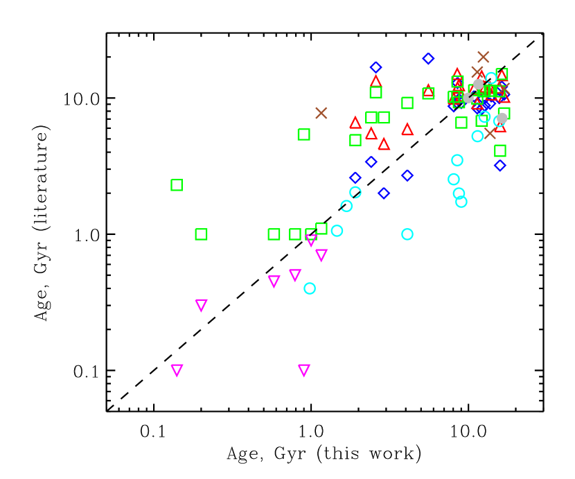
Figure 4: Comparison between our derived ages and those published in literature for GCs in M31. Each coloured-symbol correspond to a different literature work, following Table LABEL:tab_lit_m31: (a) blue diamond correspond to results by Beasley et al. (2005) (models by Bruzual & Charlot 2003); (b) red upward triangles to Beasley et al. (2005) (models by Thomas et al. 2003, 2004); (c) green squares to Puzia et al. (2005); (d) brown crosses to Fan et al. (2006); (e) magenta downward triangles to Beasley et al. (2004); (f) cyan open circles to Wang et al. (2010), and; (g) grey filled circles to Alves-Brito et al. (2009). As labeled in Table LABEL:tab_lit_m31, references (a-c) and (e) present the results based on photometric measurements, while references (d), (f) and (g) above present the results based on spectral indices. This plot is best seen in colour (online version).

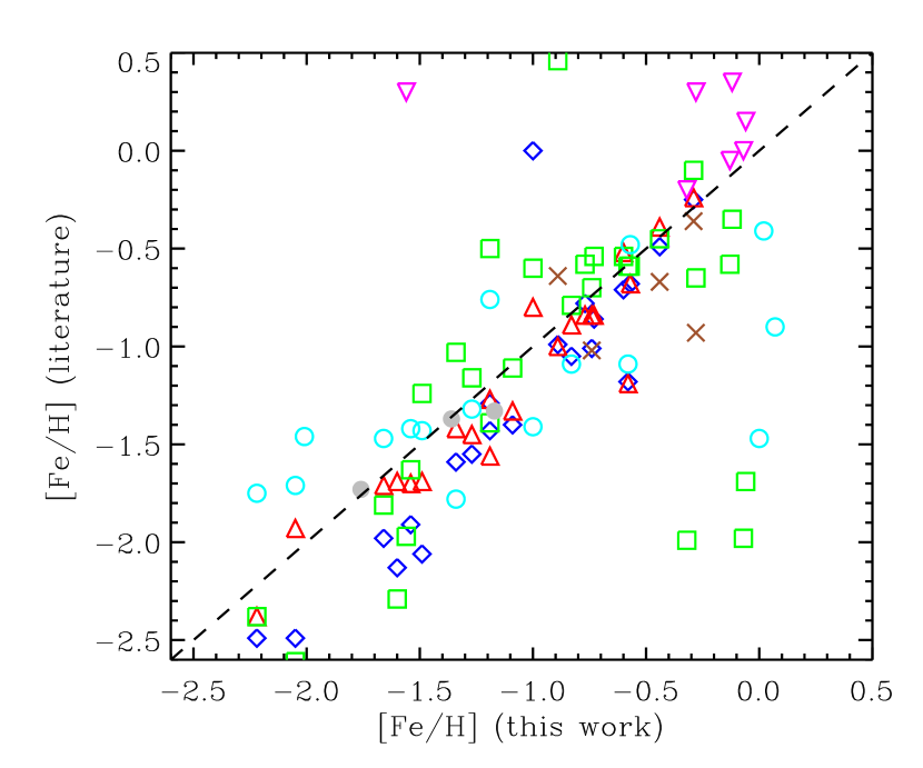
Figure 5: Comparison between our derived metallicities [Fe/H] and those published in literature for GCs in M31. The colour and symbol codes are the same as in Fig. 4. This plot is best seen in colour (online version).

Beasley et al. (2005); Puzia et al. (2005) derive [$\alpha$/Fe] values as well as age and metallicities (in our Table LABEL:tab_lit_m31 we converted their [Z/H] to [Fe/H] through equation 4 in Thomas et al. 2003). Although there has been progress in measuring abundance patterns from spectral fitting (Walcher et al., 2009) we have not attempted it in this work as the models currently available do not cover the parameter space needed. We intend to investigate this in a future work, with a larger sample.

4.3 Comparing the two GC systems

We show in Fig. 6 the age-[Fe/H] relation we obtain for our two samples, the Galactic GCs denoted by open squares and M31 GCs denoted by filled circles. It can be easily seen that the Galactic sample are consistent with old ages and a flat age-[Fe/H] relation, as expected from earlier studies on the GC system of our Galaxy. Using a sample of 54 Galactic GCs with high-quality CMDs and ages obtained photometrically, Fraix-Burnet et al. (2009) found an age-metallicity relation for the halo GCs. According to their analysis the age-[Fe/H] relation goes from [Fe/H] = –2.0 dex 12 Gyr to [Fe/H] = –1.3 dex, 9 Gyr ago. Nevertheless, their results are also consistent with a fast increase in metallicity (–1.9 $\leq$ [Fe/H] $\leq$ –1.4), at approximately 10–11 Gyr ago. More recently, Forbes & Bridges (2010) used new observations from the Hubble Space Telescope presented in Marín-Franch et al. (2009) to compile a high-quality database of 93 Galactic GCs. With the larger sample, Forbes & Bridges (2010) showed that, in fact, the Galactic GCs can be divided into two groups. The first group is an old population of GCs, compatible with a rapid formation scenario of the Galactic halo, presenting a flat age-[Fe/H] relation. The second group, however, presents some younger objects displaying an age-[Fe/H] relation which is associated with disrupted dwarf galaxies.

Figure 6: Age-metallicity relation obtained for M31 (filled circles) and Galactic GCs (open squares). Refer to the text of the paper for more details.

However, while the Galactic GCs are predominantly old, M31 shows not only young objects ($\leq$ 1 Gyr), but also a number of intermediate age and old GCs (Beasley et al., 2005; Puzia et al., 2005). These findings are also confirmed in our analysis as shown in Table 3. From Fig. 6 (filled symbols), we see that, within the uncertainties, both old GCs in the Galaxy and in M31 present similar flat age-[Fe/H] relations.

By contrast, we see that M31’s intermediate/young population (age $<$ 8 Gyr) follows a roughly linear age–[Fe/H] relation in the sense that the young GCs are also more metal-rich. These remarkable differences in age-[Fe/H] between the Galactic and M31 GC systems suggest that while the latter has likely experienced a recent, active merger history, the former has instead experienced a quiet star formation history over the last 10 Gyr (but see Forbes & Bridges, 2010, for a recent discussion on the topic). We notice, however, that a larger sample of young GCs in M31 has to be targeted to confirm (or not) the age-[Fe/H] relation we recover in this work.

The relation between the GC system’s stellar population and kinematic properties can shed light into formation of structures in a galaxy. For example, Perrett et al. (2002) investigated the kinematic properties of several hundred GCs in M31. They concluded that the metal-rich GCs present a centrally concentrated spatial distribution with a high rotation amplitude, consistent with a bulge population. Whereas the metal-poor GCs tend to be less spatially concentrated and were also found to have a strong rotation signature (see as well discussions in Huchra et al. 1991; Bekki 2010; Lee et al. 2008; Morrison et al. 2011 and references therein).

Also, the dis(similarities) between the metallicity distribution function (MDF) of the Galactic and M31 GC systems have been widely debated in literature. In Fig. 7, we present the MDF we recover from our own analysis for both systems. To our knowledge, this is the first direct comparison of [Fe/H] distributions in both Galactic and M31 GC systems employing the same methods and techniques, regardless of the GC’s position in the galaxy. In the top panel, we see that the MDF obtained from our integrated metallicities for the Galactic GCs is clearly bimodal, a result that goes back to the seminal paper by Zinn (1985), who was the first to propose the existence of two sub-populations in the Galactic GC system (see also Bica et al., 2006, for a recent discussion). The KMM mixture modelling algorithm (Ashman et al., 1994) suggests statistically convincing evidence of bimodality in the Galactic GC system (at better than the 99% confidence level).

For M31, however, the shape and distribution of the MDF is still controversial. While some authors propose that the MDF of M31 GCs presents two sub-populations – one with a metallicity peak at [Fe/H] = –1.57 that is associated to the galaxy’s halo, and other one peaking at [Fe/H] = –0.61, which is structurally associated to the galaxy’s bulge (see, e.g., Ashman & Bird, 1993; Barmby et al., 2000; Fan et al., 2008) – other authors suggest that the bimodality is not present at all or it is weakly detected (e.g. Caldwell et al., 2011).

From our own analysis for both Galactic and M31 GCs using the same methods and techniques, we obtain that both systems, regardless the age differences, cover approximately the same [Fe/H] range. Within our limited sample, the old M31 GCs extend from [Fe/H] = –2.2 up to [Fe/H] = –0.3, while the younger population goes from [Fe/H] = –2.2 up to 0.1 dex. Furthermore, the KMM algorithm applied to the old GCs in M31 does not support bimodality (the probability is less than 77%), with the number of metal-poor and metal-rich objects being almost the same in the galaxy. We note, however, that M31’s GC system is more than a factor of 2 larger than the Milky Way’s. In addition, our sample is biased not only by the number of objects studied but also by their position in the galaxy. While our sample is biased towards disk/bulge objects, more GCs in the halo of M31 need to be targeted to better understand M31’s MDF shape and properly compare it with that of the Galaxy.

Figure 7: The metallicity distribution function for (a) Galactic GCs, (b) old (ages $\geq$ 8 Gyr) M31 GCs, and (c) all (old+young) M31 GCs as analysed in this work in bins of 0.40 dex wide.

5 Summary and Conclusions

Spectroscopic ages and metallicities were derived for a sample of 38 GCs in M31, drawn from the observations of Beasley et al. (2004) and Alves-Brito et al. (2009). These parameters were obtained by fitting the observed integrated spectra to SSP models by Vazdekis et al. (2010) using the spectral fitting code ULySS (Koleva et al., 2009). To our knowledge, this is the first time that full spectrum fitting is used in deriving stellar population parameters in M31 GCs.

We tested the reliability of our analysis by fitting the integrated spectra of Galactic GCs presented in Schiavon et al. (2005). In six cases, out of 34 objects for which we obtained CMD ages from the literature, the spectroscopic ages do not match the ages drawn from CMD analysis. In the case of NGC 5286 (and possibly NGC 6752), we suspect that contamination from foreground stars hampered the observations. This is unlikely to be an issue for extra-galactic clusters. NGC 2808 is a striking case of a cluster with triple main sequences and complex HB morphology, and would deserve a more detailed modelling than SSP fitting. For the remaining four clusters, ages are underestimated by $\sim$2–3 Gyr and we cannot provide a robust explanation for these differences. We did not find evidence of a correlation with either contamination from CNONa abundance variations or a specific HB morphology.

The spectroscopic integrated metallicities derived with spectral fitting were compared to the compilations by Schiavon et al. (2005) and Carretta et al. (2009). Our results agree well with the higher resolution stellar analysis.

As for M31, we obtain a large range of ages (from $\sim$150 Myr to the age of the Universe) and metallicities (–2.2 $\leq$ [Fe/H] $\leq$ +0.1). We confirm previous results in the literature that find young globular clusters in M31, in contrast with the globular cluster system in our own Milky Way. We find an age-metallicity relation that can be described as having two components: an old population with a flat age-[Fe/H] relation, possibly associated with the halo and/or bulge in analogy to what is seen in the Milky Way, and a second one with a roughly linear relation between age and metallicity (higher metallicities corresponding to younger ages).

Finally, our analyses do not support [Fe/H] bimodality in the M31 globular cluster system, but further investigation with a larger and unbiased sample is necessary to better interpret the star formation history of M31 when compared to our own Galaxy.

Table 5: Ages and metallicities for Galactic GCs.

	Literature				This work
Cluster	Age	[Fe/H]C	[Fe/H]S		Age	[Fe/H]
	(Gyr)	(dex)	(dex)		(Gyr)	(dex)
NGC 104	13.0 $\pm$ 2.6 a	-0.76 $\pm$ 0.02	-0.70		13.09 $\pm$ 1.76	-0.79 $\pm$ 0.04
NGC 1851	10.6 $\pm$ 2.1 a	-1.18 $\pm$ 0.08	-1.21		10.26 $\pm$ 0.16	-1.26 $\pm$ 0.01
NGC 1904	11.4 $\pm$ 2.4 a	-1.58 $\pm$ 0.02	-1.55		11.58 $\pm$ 0.22	-1.84 $\pm$ 0.02
					10.24 $\pm$ 3.00	-1.88 $\pm$ 0.05
NGC 2298	12.6 $\pm$ 2.6 b	-1.96 $\pm$ 0.04	-1.97		10.89 $\pm$ 1.34	-2.00 $\pm$ 0.03
					10.32 $\pm$ 1.54	-2.06 $\pm$ 0.02
NGC 2808	10.0 $\pm$ 2.2 a	-1.18 $\pm$ 0.04	-1.29		13.90 $\pm$ 0.07	-1.24 $\pm$ 0.01
					13.87 $\pm$ 0.08	-1.25 $\pm$ 0.01
NGC 3201	13.0 $\pm$ 1.9 a	-1.51 $\pm$ 0.02	-1.56		9.56 $\pm$ 0.24	-1.35 $\pm$ 0.01
					11.75 $\pm$ 0.11	-1.45 $\pm$ 0.01
NGC 5286	12.5 $\pm$ 2.5 b	-1.70 $\pm$ 0.07	-1.51		6.04 $\pm$ 4.46	-1.78 $\pm$ 0.08
					9.19 $\pm$ 3.34	-1.79 $\pm$ 0.07
					4.01 $\pm$ 2.97	-1.66 $\pm$ 0.07
NGC 5904	10.6 $\pm$ 2.2 a	-1.33 $\pm$ 0.02	-1.26		9.26 $\pm$ 0.11	-1.44 $\pm$ 0.00
					10.00 $\pm$ 0.16	-1.41 $\pm$ 0.01
NGC 5927	12.1 $\pm$ 2.4 a	-0.29 $\pm$ 0.07	-0.64		11.38 $\pm$ 2.54	-0.48 $\pm$ 0.04
					12.87 $\pm$ 1.73	-0.50 $\pm$ 0.02
					12.77 $\pm$ 1.37	-0.48 $\pm$ 0.02
NGC 5946	11.7 $\pm$ 3.0 a	-1.29 $\pm$ 0.14	-1.54		10.56 $\pm$ 1.93	-1.76 $\pm$ 0.04
NGC 5986	11.6 $\pm$ 2.3 a	-1.63 $\pm$ 0.08	-1.53		10.14 $\pm$ 3.33	-1.84 $\pm$ 0.05
NGC 6121	11.9 $\pm$ 2.3 a	-1.18 $\pm$ 0.02	-1.15		7.94 $\pm$ 0.14	-1.35 $\pm$ 0.01
NGC 6171	13.0 $\pm$ 2.7 a	-1.03 $\pm$ 0.02	-1.13		13.22 $\pm$ 1.27	-1.07 $\pm$ 0.03
					12.23 $\pm$ 1.47	-1.05 $\pm$ 0.03
NGC 6218	12.1 $\pm$ 2.5 a	-1.33 $\pm$ 0.02	-1.32		11.08 $\pm$ 0.94	-1.63 $\pm$ 0.02
NGC 6235	11.7 $\pm$ 3.0 a	-1.38 $\pm$ 0.07	-1.36		9.81 $\pm$ 1.07	-1.26 $\pm$ 0.04
NGC 6254	11.3 $\pm$ 2.3 a	-1.57 $\pm$ 0.02	-1.51		11.73 $\pm$ 0.05	-1.72 $\pm$ 0.02
NGC 6266	12.1 $\pm$ 2.4 a	-1.18 $\pm$ 0.07	-1.20		10.60 $\pm$ 0.10	-1.22 $\pm$ 0.01
NGC 6284	11.4 $\pm$ 2.3 a	-1.31 $\pm$ 0.09	-1.27		10.21 $\pm$ 0.12	-1.33 $\pm$ 0.01
					10.39 $\pm$ 0.48	-1.28 $\pm$ 0.02
NGC 6304	13.5 $\pm$ 2.8 b	-0.37 $\pm$ 0.07	-0.66		14.69 $\pm$ 3.43	-0.63 $\pm$ 0.06
NGC 6316		-0.36 $\pm$ 0.14	-0.90		14.83 $\pm$ 0.93	-0.86 $\pm$ 0.02
					14.46 $\pm$ 1.30	-0.86 $\pm$ 0.03
NGC 6333		-1.79 $\pm$ 0.09	-1.65		10.49 $\pm$ 2.17	-2.03 $\pm$ 0.03
NGC 6342	12.3 $\pm$ 2.5 a	-0.49 $\pm$ 0.14	-1.01		13.13 $\pm$ 0.47	-0.93 $\pm$ 0.01
					12.95 $\pm$ 0.85	-0.84 $\pm$ 0.02
NGC 6352	12.6 $\pm$ 2.6 b	-0.62 $\pm$ 0.05	-0.70		12.24 $\pm$ 0.35	-0.70 $\pm$ 0.01
NGC 6356		-0.35 $\pm$ 0.14	-0.74		14.26 $\pm$ 2.10	-0.76 $\pm$ 0.04
NGC 6362	12.1 $\pm$ 2.4 a	-1.07 $\pm$ 0.05	-1.17		14.53 $\pm$ 0.21	-1.22 $\pm$ 0.01
NGC 6388	12.0 $\pm$ 2.6 b	-0.45 $\pm$ 0.04	-0.68		6.57 $\pm$ 1.10	-0.62 $\pm$ 0.03
NGC 6441	11.2 $\pm$ 2.4 b	-0.44 $\pm$ 0.07	-0.65		6.09 $\pm$ 1.80	-0.55 $\pm$ 0.04
					5.89 $\pm$ 0.67	-0.54 $\pm$ 0.02
NGC 6522		-1.45 $\pm$ 0.08	-1.39		8.97 $\pm$ 0.43	-1.24 $\pm$ 0.02
NGC 6528	12.6 $\pm$ 2.5 c	0.07 $\pm$ 0.08	-0.10		13.60 $\pm$ 1.42	-0.29 $\pm$ 0.03
					12.39 $\pm$ 1.95	-0.26 $\pm$ 0.04
NGC 6544	10.6 $\pm$ 2.3 a	-1.47 $\pm$ 0.07	-1.38		11.57 $\pm$ 0.91	-1.34 $\pm$ 0.02
NGC 6553	13.0 $\pm$ 2.5 d	-0.16 $\pm$ 0.06	-0.20		10.35 $\pm$ 4.23	-0.29 $\pm$ 0.08
NGC 6569		-0.72 $\pm$ 0.14	-1.08		14.98 $\pm$ 0.15	-1.06 $\pm$ 0.01
NGC 6624	12.5 $\pm$ 2.6 b	-0.42 $\pm$ 0.07	-0.70		9.21 $\pm$ 1.53	-0.70 $\pm$ 0.04
					11.21 $\pm$ 1.71	-0.74 $\pm$ 0.04
NGC 6626		-1.46 $\pm$ 0.09	-1.21		10.39 $\pm$ 0.68	-1.37 $\pm$ 0.02
NGC 6637	11.9 $\pm$ 2.6 a	-0.59 $\pm$ 0.07	-0.78		13.38 $\pm$ 1.34	-0.86 $\pm$ 0.03
NGC 6638		-0.99 $\pm$ 0.07	-1.08		12.96 $\pm$ 1.21	-1.00 $\pm$ 0.02
NGC 6652	12.1 $\pm$ 2.5 a	-0.76 $\pm$ 0.14	-1.10		11.72 $\pm$ 0.28	-0.95 $\pm$ 0.01
					10.12 $\pm$ 0.15	-1.01 $\pm$ 0.01
NGC 6723	12.7 $\pm$ 2.9 a	-1.10 $\pm$ 0.07	-1.14		12.78 $\pm$ 0.15	-1.34 $\pm$ 0.01
NGC 6752	13.5 $\pm$ 2.9 a	-1.55 $\pm$ 0.01	-1.57		9.37 $\pm$ 3.75	-1.86 $\pm$ 0.07
NGC 7078	12.5 $\pm$ 2.6 a	-2.33 $\pm$ 0.02	–		6.82 $\pm$ 1.43	-2.32 $\pm$ 0.01
					6.98 $\pm$ 1.19	-2.32 $\pm$ 0.01
NGC 7089	11.9 $\pm$ 2.7 a	-1.66 $\pm$ 0.07	-1.49		10.36 $\pm$ 2.89	-1.82 $\pm$ 0.06

Table 5: continued.

Table 6: Ages and metallicities from literature, for our sample of M31 GCs.

Cluster	Age	[Fe/H]	Method	Reference
	(Gyr)	(dex)
B126	3.40 $\pm$ 1.00	-1.43 $\pm$ 0.42	Spectral indices	a
	5.50 $\pm$ 3.50	-1.56 $\pm$ 0.24	Spectral indices	b
	7.20 $\pm$ 3.10	-1.39 $\pm$ 0.28	Spectral indices	c
B134	9.10 $\pm$ 2.20	-0.99 $\pm$ 0.48	Spectral indices	a
	11.90 $\pm$ 1.90	-1.00 $\pm$ 0.38	Spectral indices	b
	11.30 $\pm$ 1.80	0.46 $\pm$ 0.11	Spectral indices	c
	5.50 $\pm$ 2.28	-0.64 $\pm$ 0.08	Photometry	d
B158	9.90 $\pm$ 2.70	-1.01 $\pm$ 0.24	Spectral indices	a
	12.10 $\pm$ 0.90	-0.84 $\pm$ 0.18	Spectral indices	b
	11.30 $\pm$ 1.50	-0.70 $\pm$ 0.08	Spectral indices	c
	20.00 $\pm$ 5.57	-1.02 $\pm$ 0.02	Photometry	d
B163	10.60 $\pm$ 3.70	-0.25 $\pm$ 0.27	Spectral indices	a
	10.20 $\pm$ 4.80	-0.24 $\pm$ 0.22	Spectral indices	b
	7.70 $\pm$ 1.00	-0.10 $\pm$ 0.06	Spectral indices	c
	11.75 $\pm$ 1.60	-0.36 $\pm$ 0.27	Photometry	d
B222	0.70 $\pm$ 0.70	0.30 $\pm$ 0.60	Spectral indices	e
	1.10 $\pm$ 0.40	-0.65 $\pm$ 0.18	Spectral indices	c
	7.75 $\pm$ 1.46	-0.93 $\pm$ 0.95	Photometry	d
B225	8.40 $\pm$ 1.90	-0.49 $\pm$ 0.14	Spectral indices	a
	9.10 $\pm$ 1.20	-0.39 $\pm$ 0.18	Spectral indices	b
	9.90 $\pm$ 1.20	-0.45 $\pm$ 0.05	Spectral indices	c
	15.50 $\pm$ 4.89	-0.67 $\pm$ 0.12	Photometry	d
B234	10.30 $\pm$ 3.20	-0.86 $\pm$ 0.18	Spectral indices	a
	11.70 $\pm$ 5.70	-0.84 $\pm$ 0.19	Spectral indices	b
	11.40 $\pm$ 2.00	-0.54 $\pm$ 0.10	Spectral indices	c
B292	2.70 $\pm$ 1.20	-1.91 $\pm$ 0.58	Spectral indices	a
	5.90 $\pm$ 3.40	-1.70 $\pm$ 0.20	Spectral indices	b
	9.20 $\pm$ 3.30	-1.63 $\pm$ 0.49	Spectral indices	c
	1.00 $\pm$ 0.10	-1.42 $\pm$ 0.16	Photometry	f
B301	3.20 $\pm$ 1.80	-1.29 $\pm$ 0.31	Spectral indices	a
	6.20 $\pm$ 1.10	-1.27 $\pm$ 0.55	Spectral indices	b
	4.10 $\pm$ 3.70	-0.50 $\pm$ 0.26	Spectral indices	c
		-0.76 $\pm$ 0.25	Photometry	f
B304	12.90 $\pm$ 4.70	-1.55 $\pm$ 0.65	Spectral indices	a
	11.90 $\pm$ 3.90	-1.45 $\pm$ 0.43	Spectral indices	b
	13.20 $\pm$ 3.10	-1.16 $\pm$ 0.46	Spectral indices	c
		-1.32 $\pm$ 0.22	Photometry	f
B305	0.40 $\pm$ 0.10	-0.90 $\pm$ 0.61	Photometry	f
B307	1.61 $\pm$ 0.10	-0.41 $\pm$ 0.36	Photometry	f
B310	19.50 $\pm$ 2.10	-2.06 $\pm$ 0.51	Spectral indices	a
	11.40 $\pm$ 3.50	-1.69 $\pm$ 0.47	Spectral indices	b
	10.80 $\pm$ 3.10	-1.24 $\pm$ 0.52	Spectral indices	c
		-1.43 $\pm$ 0.28	Photometry	f
B313	8.80 $\pm$ 1.20	-1.05 $\pm$ 0.35	Spectral indices	a
	11.70 $\pm$ 0.90	-0.89 $\pm$ 0.50	Spectral indices	b
	11.20 $\pm$ 1.20	-0.79 $\pm$ 0.32	Spectral indices	c
	7.28 $\pm$ 0.70	-1.09 $\pm$ 0.10	Photometry	f
B314	0.50 $\pm$ 0.60	0.35 $\pm$ 0.25	Spectral indices	e
	1.00 $\pm$ 0.10	-0.35 $\pm$ 0.22	Spectral indices	c
B316	1.06 $\pm$ 0.10	-1.47 $\pm$ 0.23	Photometry	f
B321	0.30 $\pm$ 0.30	0.00 $\pm$ 0.60	Spectral indices	e
	1.00 $\pm$ 0.10	-1.98 $\pm$ 0.30	Spectral indices	c
B322	0.10 $\pm$ 0.50	-0.20 $\pm$ 0.20	Spectral indices	e
	2.30 $\pm$ 0.70	-1.99 $\pm$ 0.43	Spectral indices	c
B324	0.90 $\pm$ 0.20	-0.05 $\pm$ 0.40	Spectral indices	e
	1.00 $\pm$ 0.10	-0.58 $\pm$ 0.20	Spectral indices	c
B327	0.10 $\pm$ 0.90	0.30 $\pm$ 0.75	Spectral indices	e
	5.40 $\pm$ 1.40	-1.97 $\pm$ 0.34	Spectral indices	c
B328	16.80 $\pm$ 5.20	-2.13 $\pm$ 0.35	Spectral indices	a
	13.30 $\pm$ 1.30	-1.69 $\pm$ 0.35	Spectral indices	b
	11.00 $\pm$ 2.40	-2.29 $\pm$ 0.42	Spectral indices	c
B337	2.60 $\pm$ 1.90	-1.18 $\pm$ 0.19	Spectral indices	a
	6.60 $\pm$ 3.20	-1.19 $\pm$ 0.25	Spectral indices	b
	4.90 $\pm$ 2.90	-0.59 $\pm$ 0.11	Spectral indices	c
	2.03 $\pm$ 0.10	-1.09 $\pm$ 0.32	Photometry	f
B347	8.70 $\pm$ 5.70	-2.49 $\pm$ 0.21	Spectral indices	a
	9.90 $\pm$ 4.00	-1.93 $\pm$ 0.51	Spectral indices	b
	10.20 $\pm$ 2.40	-2.61 $\pm$ 0.37	Spectral indices	c
	2.53 $\pm$ 0.15	-1.71 $\pm$ 0.03	Photometry	f
B350	9.80 $\pm$ 2.50	-1.98 $\pm$ 0.49	Spectral indices	a
	12.40 $\pm$ 4.70	-1.71 $\pm$ 0.33	Spectral indices	b
	9.30 $\pm$ 2.30	-1.81 $\pm$ 0.37	Spectral indices	c
	1.99 $\pm$ 0.10	-1.47 $\pm$ 0.17	Photometry	f
B354	5.24 $\pm$ 0.65	-1.46 $\pm$ 0.38	Photometry	f
B365	9.20 $\pm$ 3.10	-1.59 $\pm$ 0.44	Spectral indices	a
	10.40 $\pm$ 2.20	-1.42 $\pm$ 0.51	Spectral indices	b
	6.60 $\pm$ 3.10	-1.03 $\pm$ 0.20	Spectral indices	c
	1.73 $\pm$ 0.10	-1.78 $\pm$ 0.19	Photometry	f
B380	0.45 $\pm$ 0.13	0.15 $\pm$ 0.10	Spectral indices	e
	1.00 $\pm$ 0.10	-1.69 $\pm$ 0.13	Spectral indices	c
B383	10.30 $\pm$ 2.20	-0.68 $\pm$ 0.18	Spectral indices	a
	10.60 $\pm$ 1.30	-0.68 $\pm$ 0.31	Spectral indices	b
	11.30 $\pm$ 2.40	-0.59 $\pm$ 0.08	Spectral indices	c
	13.99 $\pm$ 1.05	-0.48 $\pm$ 0.20	Photometry	f
B393	10.00 $\pm$ 1.80	0.00 $\pm$ 0.00	Spectral indices	a
	11.90 $\pm$ 1.30	-0.80 $\pm$ 0.47	Spectral indices	b
	11.20 $\pm$ 1.40	-0.60 $\pm$ 0.14	Spectral indices	c
	6.76 $\pm$ 1.10	-1.41 $\pm$ 0.05	Photometry	f
B398	12.10 $\pm$ 1.50	-0.71 $\pm$ 0.41	Spectral indices	a
	14.70 $\pm$ 3.70	-0.52 $\pm$ 0.28	Spectral indices	b
	15.00 $\pm$ 2.40	-0.54 $\pm$ 0.10	Spectral indices	c
B401	9.20 $\pm$ 5.80	-2.49 $\pm$ 0.49	Spectral indices	a
	15.00 $\pm$ 5.10	-2.38 $\pm$ 0.24	Spectral indices	b
	10.20 $\pm$ 2.40	-2.38 $\pm$ 0.32	Spectral indices	c
	3.49 $\pm$ 0.40	-1.75 $\pm$ 0.29	Photometry	f
MGC1	7.10 $\pm$ 3.00	-1.37 $\pm$ 0.15	Spectral indices	g
MCGC5	10.00 $\pm$ 3.00	-1.33 $\pm$ 0.12	Spectral indices	g
MCGC10	12.60 $\pm$ 3.00	-1.73 $\pm$ 0.20	Spectral indices	g
NB16	2.00 $\pm$ 1.40	-1.40 $\pm$ 0.18	Spectral indices	a
	4.60 $\pm$ 0.80	-1.33 $\pm$ 0.24	Spectral indices	b
	7.20 $\pm$ 3.50	-1.11 $\pm$ 0.15	Spectral indices	c
NB89	8.30 $\pm$ 2.60	-0.78 $\pm$ 0.14	Spectral indices	a
	14.40 $\pm$ 2.70	-0.84 $\pm$ 0.15	Spectral indices	b
	6.80 $\pm$ 1.70	-0.58 $\pm$ 0.08	Spectral indices	c

Table 6: continued.

References for column 5: (a) Beasley et al. (2005) (models by Bruzual & Charlot 2003); (b) Beasley et al. (2005) (models by Thomas et al. 2003, 2004); (c) Puzia et al. (2005); (d) Fan et al. (2006); (e) Beasley et al. (2004); (f) Wang et al. (2010), and; (g) Alves-Brito et al. (2009). Regarding the references (a), (b) and (c), we converted their [Z/H] to [Fe/H] through equation 4 in Thomas et al. (2003). Notes: We did not find in the listed literature the parameters for two clusters in our sample, B302 and B331.