Generalized fiducial inference for normal linear mixed models

Abstract

While linear mixed modeling methods are foundational concepts introduced in any statistical education, adequate general methods for interval estimation involving models with more than a few variance components are lacking, especially in the unbalanced setting. Generalized fiducial inference provides a possible framework that accommodates this absence of methodology. Under the fabric of generalized fiducial inference along with sequential Monte Carlo methods, we present an approach for interval estimation for both balanced and unbalanced Gaussian linear mixed models. We compare the proposed method to classical and Bayesian results in the literature in a simulation study of two-fold nested models and two-factor crossed designs with an interaction term. The proposed method is found to be competitive or better when evaluated based on frequentist criteria of empirical coverage and average length of confidence intervals for small sample sizes. A MATLAB implementation of the proposed algorithm is available from the authors.

and

t2Supported in part by NSF Grants DMS-07-07037, DMS-10-07543 and DMS-10-16441.

1 Introduction

Inference on parameters of normal linear mixed models has an extensive history; see Khuri and Sahai (1985) for a survey of variance component methodology, or Chapter 2 of Searle, Casella and McCulloch (1992) for a summary. There are many inference methods for variance components such as ANOVA-based methods [Burdick and Graybill (1992), Hernandez, Burdick and Birch (1992), Hernandez and Burdick (1993), Jeyaratnam and Graybill (1980)], maximum likelihood estimation (MLE) and restricted maximum likelihood (REML) [Hartley and Rao (1967), Searle, Casella and McCulloch (1992)] along with Bayesian methods [Gelman (2006), Gelman et al. (2004), Wolfinger and Kass (2000)]. Many of the ANOVA-based methods become quite complex with complicated models (e.g., due to nesting or crossing data structures), and are not guaranteed to perform adequately when the designs become unbalanced. When the model design is not balanced, the decomposition of the sum-of-squares for ANOVA-based methods is not generally unique, chi-squared or independent. Furthermore, “exact” ANOVA-based confidence intervals are typically for linear combinations of variance components, but not the individual variance components even for simple models [Burdick and Graybill (1992), pages 67 and 68, Jiang (2007)]; however, approximate intervals do exist. With notable optimality properties for point estimation, MLE and REML methods are less useful when it comes to confidence interval estimation for small samples because the asymptotic REML-based confidence intervals tend to have lower than stated empirical coverage [Burch (2011), Burdick and Graybill (1992), Searle, Casella and McCulloch (1992)]. Bayesian methods, in particular, hierarchical modeling, can be an effective resolution to complicated models, but the delicate question of selecting appropriate prior distributions must be addressed.

There are numerous applications of normal linear mixed models related to topics such as animal breeding studies [Burch and Iyer (1997), E, Hannig and Iyer (2008)], multilevel studies [O’Connell and McCoach (2008)] and longitudinal studies [Laird and Ware (1982)]. Many implemented methods do not go beyond two variance components or are designed for a very specific setting. We propose a solution based on generalized fiducial inference that easily allows for inference beyond two variance components and for the general normal linear mixed model settings.

The proposed generalized fiducial approach is designed specifically for interval data (e.g., due to the measuring instrument’s resolution, rounding for storage on a computer or bid-ask spread in financial data). There are several reasons to consider interval data. First, there are many examples where it is critical [or required per the regulations outlined in GUM (1995)] to incorporate all known sources of uncertainty [Elster (2000), Frenkel and Kirkup (2005), Hannig, Iyer and Wang (2007), Lira and Woger (1997), Taraldsen (2006), Willink (2007)]. Second, our simulation results for the normal linear mixed model show that even when considering this extra source of uncertainty, the proposed method is competitive or better than classical and Bayesian methods that assume the data are exact; see Section 3. [The proposed method is also appropriate for noninterval, or standard, data simply by artificially discretizing the observation space into a fixed grid of narrow intervals; Hannig (2012) proves that as the interval width decreases to zero, the generalized fiducial distribution converges to the generalized fiducial distribution for exact data.] Finally, on a purely philosophical level, all continuous data has some degree of uncertainty, as noted previously, due to the resolution of the measuring instrument or truncation for storage on a computer. Note that we are not suggesting that all methods should incorporate this known uncertainty; however, we were able to appeal to this known uncertainty for the computational aspect of the proposed method.

A general form of a normal linear mixed model is

$$Y=\mathbf{X}\beta+\mathbf{V}Z+\varepsilon,$$ (1)

where $Y$ is an $n\times 1$ vector of data, $\mathbf{X}$ is a known $n\times p$ fixed effects design matrix, $\beta$ is a $p\times 1$ vector of unknown fixed effects, $\mathbf{V}Z=\sum_{i=1}^{r-1}\mathbf{V}_{i}Z_{i}$, where $Z_{i}$ is a vector of effects representing each level of random effect $i$ such that $E(Z_{i})=0$ and $\operatorname{var}(Z_{i})=\mathbf{G}$, $\mathbf{V}_{i}$ is the known design matrix for random effect $i$, and $\varepsilon$ is an $n\times 1$ vector representing the error and $E(\varepsilon)=0$ and $\operatorname{var}(\varepsilon)=\mathbf{R}$ [Jiang (2007)]. Note that there are $r$ total random components in this model, and covariance matrices $\mathbf{G}$ and $\mathbf{R}$ contain unknown parameters known as variance components. It is often assumed that $\mathbf{Z}$ and $\varepsilon$ are independent and normally distributed. Additional assumptions on this model for the proposed method are addressed in Section 2.

Except where noted, the notational convention that will be used for matrices, vectors, and single values will be, respectively, bold and capital letters for matrices, capital letters for vectors and lowercase letters for single values (e.g., $\mathbf{A}$, $A$, $a$).

The focus of this paper is the construction of confidence intervals for the unknown parameters of (1), with emphasis on the variance components of matrices $\mathbf{G}$ and $\mathbf{R}$. In this paper, inferences are derived from the generalized fiducial distributions of the unknown parameters, and we propose a sequential Monte Carlo (SMC) algorithm to obtain these samples. Like a Bayesian posterior, this procedure produces a distribution on the parameter space, but does so without assuming a prior distribution. We evaluate the quality of the simulated generalized fiducial distribution based on the quality of the confidence intervals—a concept analogous to confidence distributions [Schweder and Hjort (2002), Xie, Singh and Strawderman (2011)]. We begin by introducing the two main techniques of the proposed method: generalized fiducial inference and SMC methods. Then we introduce the proposed method, and state and prove a theorem concluding the convergence of the algorithm. To demonstrate small sample performance, we perform a simulation study on two different types of models (unbalanced two-fold nested models and two-factor crossed with interaction models), and include a real-data application for the two-fold nested model. We finish with concluding remarks. Additional information can be found in the supplemental document [Cisewski and Hannig (2012)].

1.1 Generalized fiducial inference

Fiducial inference was introduced by Fisher (1930) to rectify what he saw as a weakness in the Bayesian philosophy, where a prior distribution is assumed without sufficient prior knowledge. While Fisher made several attempts at justifying his definition of fiducial inference [Fisher (1933, 1935)], it was not fully developed. Fiducial inference fell into disrepute when it was discovered that some of the properties Fisher claimed did not hold [Lindley (1958), Zabell (1992)]. Efforts were made to revitalize fiducial inference by drawing connections to other areas such as Fraser’s structural inference [Fraser (1961a, 1961b, 1966, 1968)], and more recently Hannig, Iyer and Patterson (2006) connect Fisher’s fiducial inference to generalized inference introduced in Tsui and Weerahandi (1989) and Weerahandi (1993). In this paper, we propose a method for inference on parameters of normal linear mixed models using the ideas of generalized fiducial inference.

The main idea of fiducial inference is a transference of randomness from the model space to the parameter space. A thorough introduction to generalized fiducial inference can be found in Hannig (2009), but here we consider a simple example. Let $y$ be a realization of a random variable $Y\sim N(\mu,1)$ [where $N(\mu,1)$ represents a normal distribution with unknown mean $\mu$ and standard deviation 1]. The random variable $Y$ can be represented as $Y=\mu+Z$ where $Z\sim N(0,1)$. Given the observed value $y$, the fiducial argument solves this equation for the unknown parameter $\mu$ to get $\mu=y-Z$; for example, suppose $y=4.8$, then $\mu=4.8-Z$ would suggest $\mu\sim N(4.8,1)$. While the actual value of $Z$ is unknown, the distribution of $Z$ is fully known and can be used to frame a distribution on the unknown parameter $\mu$. This distribution on $\mu$ is known as the fiducial distribution.

The generalized fiducial recipe starts with a data-generating equation, also referred to as the structural equation, which defines the relationship between the data and the parameters. Let $Y$ be a random vector indexed by parameter(s) $\xi\in\Xi$, and then assume $Y$ can be represented as $Y=G(\xi,{U})$, where $G$ is a jointly measurable function indicating the structural equation, and $U$ is a random element with a fully known distribution (void of unknown parameters). In this paper, the function $G$ will take the form of a normal linear mixed model, and the random components $U$ will be standard normal random variables; see equation (3). Following the fiducial argument, we define a set-valued function, the inverse image of $G$, as $Q({\mathbf{y}},{\mathbf{u}})=\{\xi\dvtx{\mathbf{y}}=G(\xi,{\mathbf{u}})\}$, where ${\mathbf{y}}$ is the observed data, and ${\mathbf{u}}$ is an arbitrary realization of ${U}$. The set-function $Q({\mathbf{y}},{\mathbf{u}})$ is then used to define the fiducial distribution on the parameter space. Since the distribution of ${U}$ is completely known, independent copies of $U$, $U^{*}$, can be generated to produce a random sample of $Q({\mathbf{y}},{\mathbf{u}}^{*})$ for the given data ${\mathbf{y}}$ (where ${\mathbf{u}}^{*}$ is a realization of $U^{*}$). There are several sources of nonuniqueness in this framework. In particular, nonuniqueness could occur if $Q$ has more than one element, if $Q$ is empty, or due to the definition of the structural equation. Nonuniqueness due to the definition of the structural equation will not be addressed here as we assume the form of the model is known (i.e., normal linear mixed model). To resolve the case when there is more than one element in $Q$, we can define a rule, call it $V$, for selecting an element of $Q$. Furthermore, since the parameters $\xi$ are fixed but unknown, there must be some realization of the random variable $U$ such that ${\mathbf{y}}=G(\xi,{\mathbf{u}})$ has occurred [i.e., $\{Q({\mathbf{y}},{\mathbf{u}})\neq\varnothing\}$]. The generalized fiducial distribution of $\xi$ is defined as

$$V\bigl{(}Q\bigl{(}{\mathbf{y}},U^{*}\bigr{)}\bigr{)}\mid\bigl{\{}Q\bigl{(}{\mathbf{y}},U^{*}\bigr{)}\neq\varnothing\bigr{\}}.$$ (2)

Obtaining a random sample from the generalized fiducial distribution as defined in (2) where the structural equation, $G$, takes the form of a normal linear mixed model is the focus of the proposed algorithm.

Defining the generalized fiducial distribution as (2) leads to a potential source of nonuniqueness due to conditioning on events with zero probability [i.e., if $P(\{Q(\mathbf{y},\mathbf{u})\neq\varnothing\})=0$]. This is known as the Borel Paradox [Casella and Berger (2002)]. Fortunately this can be resolved by noting that most data has some degree of known uncertainty due, for example, to the resolution of the instrument collecting the data or computer storage. Because of this, instead of considering the value of a datum, an interval around the value can be used [Hannig (2012), Hannig, Iyer and Wang (2007)]. For example, suppose the datum value is $y=1.632$ meters measuring the height of a woman. If the resolution of the instrument used to measure the woman is $0.001$ m (i.e., $1$ mm), then her actual height is between $1.631$ meters and $1.632$ meters (or between $1.632$ meters and $1.633$ meters, depending on the practice of the measurer).

By considering interval data, the issue of nonuniqueness due to the Borel Paradox is resolved since the probability of observing our data will never be zero since $P(Q((a,b),U^{*})\neq\varnothing)\geq P(Y\in(a,b))>0$ where $a<b$ are the endpoints of the interval.

Interval data is not explicitly required for generalized fiducial inference, but is useful in the proposed setting of normal linear mixed models. Generalized fiducial inference has a number of other applications in various settings such as wavelet regression [Hannig and Lee (2009)], confidence intervals for extremes [Wandler and Hannig (2012)], metrology [Hannig, Iyer and Wang (2007)] and variance component models [E, Hannig and Iyer (2008)], which applies the generalized fiducial framework to unbalanced normal linear mixed models with two variance components.

1.2 Sequential Monte Carlo

When integrals of interest are very complex or unsolvable by analytical methods, simulation-based methods can be used. SMC, or particle filters, is a collection of simulation methods used to sample from an evolving target distribution (i.e., the distribution of interest) accomplished by propagating a system of weighted particles through time or some other index. A solid introduction of and applications to SMC methods can be found in Doucet, de Freitas and Gordon (2001). There are many dimensions to the theory and applications of SMC algorithms [Chopin (2002, 2004), Del Moral, Doucet and Jasra (2006), Douc and Moulines (2008), Kong, Liu and Wong (1994), Liu and Chen (1998), Liu and West (2001)], but a simplified introduction is presented below.

Suppose one desires to make inferences about some population based on data $Y$. A particle system $\{z^{(J)},w^{(J)}\}$ for $J=1,\ldots,N$ particles is a collection of $N$ weighted random variables (with weights $w^{(J)}$) such that

$$\lim_{N\longrightarrow\infty}\frac{\sum_{J=1}^{N}w^{(J)}\gamma(z^{(J)})}{\sum_{J=1}^{N}w^{(J)}}\longrightarrow E_{\pi}\bigl{\{}\gamma(z)\bigr{\}}=\int\gamma(z)\,d\pi(z),$$

where $\pi$ is the target distribution, and $\gamma$ is some measurable function, when this expectation exists. Since it is often difficult to sample directly from the target distribution $\pi$, it becomes necessary to find some proposal distribution $\widetilde{\pi}$ to sample the particles. The weights $w^{(J)}$ are determined in order to re-weight the sampled particles back to the target density [i.e., $w^{(J)}=\pi(z^{(J)})/\widetilde{\pi}(z^{(J)})$]. This is the general idea of importance sampling (IS). If the target distribution is evolving with some time index, an iterative approach to calculating the weights is performed. This is known as sequential importance sampling (SIS). Unfortunately, with each time step, more variation is incorporated into the particle system, and the weights degenerate, leaving most particles with weights of essentially zero. The degeneracy is often measured by the effective sample size (ESS), which is a measure of the distribution of the weights of the particles. Kong, Liu and Wong (1994) presents the ESS as having an inverse relation with the coefficient of variation of the particle weights, and proved that this coefficient of variation increases as the time index increases (i.e., as more data becomes available) in the SIS setting. An intuitive explanation of ESS can be found in Liu and Chen (1995).

SMC builds on ideas of sequential importance sampling (SIS) by incorporating a resampling step to resolve issues with the degeneracy of the particle system. Once the ESS for the particle system has dropped below some designated threshold or at some pre-specified time, the particle system is resampled, removing inefficient particles with low weights and replicating the particles with higher weights [Liu and Chen (1995)]. There are various methods for resampling with the most basic being multinomial resampling, which resamples particles based on the normalized importance weights; see Douc, Cappé and Moulines (2005) for a comparison of several resampling methods.

Examples of general SMC algorithms can be found in Del Moral, Doucet and Jasra (2006) or Jasra, Stephens and Holmes (2007). The main idea of SMC methods is to iteratively target a sequence of distributions $\{\pi_{t}\}_{t\in\mathbf{Z}^{+}}$, where $\pi_{t}$ is often some distribution based on the data available up to time $t$. The algorithm comprises three main sections after the initialization step: sampling, correction and resampling. The sampling step arises at a new time step $t$ when particles are sampled from some evolving proposal distribution $\widetilde{\pi}_{t}$. The correction step is concerned with the calculation of the weights and the idea of reweighting the particles to target the desired distribution at time $t$, $\pi_{t}$. The resampling step is performed when the ESS of the particle system falls below some desired threshold $T$ (e.g., $T=N/2$). The asymptotic correctness for SMC algorithms can be found in Douc and Moulines (2008).

2 Method

2.1 Introduction

The form of the normal linear mixed model from equation (1) is adapted to work in the generalized fiducial inference setting as

$$\mathbf{Y}=\mathbf{X}\beta+\sum_{i=1}^{r}\sigma_{i}\sum_{j=1}^{l_{i}}V_{i,j}z_{i,j},$$ (3)

where $\mathbf{X}$ is a known $n\times p$ fixed-effects design matrix, $\beta$ is the $p\times 1$ vector of fixed effects, $V_{i,j}$ is the $n\times 1$ design vector for level $j$ of random effect $i$, $l_{i}$ is the number of levels per random effect $i$, $\sigma_{i}^{2}$ is the variance of random effect $i$ and the $z_{i,j}$ are independent and identically distributed standard normal random variables. We will derive a framework for inference on the unknown parameters ($\beta$ and $\sigma_{i},i=1,\ldots,r$) of this model, which will be applicable to both the balanced and the unbalanced case. (The design is balanced if there is an equal number of observations in each level of each effect, otherwise the design is unbalanced.) In addition, the covariance matrices for the random components ($\mathbf{G}$ and $\mathbf{R}$ above) are identity matrices with a rank equal to the number of levels of its corresponding random effect with $l_{r}=n$. The $\mathbf{V}_{i}$, $i=1,\ldots,r$, allow for coefficients for the random effects, and correlation structure can be incorporated into the model by including additional effects with design matrices that account for the correlation. We note that these additional assumptions are related to the implementation of the proposed algorithm, and are not restrictions of the generalized fiducial framework.

Consider the following example illustrating the connection between (1) and (3) in the case of a one-way random effects model. A one-way random effects model is conventionally written as

$$y_{ij}=\mu+\alpha_{i}+\varepsilon_{ij},\qquad i=1,\ldots,a,j=1,\ldots,n_{i},$$ (4)

with unknown mean $\mu$, random effect $\alpha\sim N(0,\sigma_{\alpha}^{2})$ where $\sigma_{\alpha}^{2}$ is unknown, $a$ is the number of levels of $\alpha$, $n_{i}$ is the number of observations in level $i$ and error terms $\varepsilon_{ij}\sim N(0,\sigma_{\varepsilon}^{2})$ where $\sigma_{\varepsilon}^{2}$ is also unknown, and $\alpha$ and $\varepsilon$ are independent [Jiang (2007)]. This can be structured in the form of equation (3) as

$$\mathbf{Y}=\mathbf{X}\beta+\sigma_{1}\sum_{j=1}^{l_{1}}V_{1,j}z_{1,j}+\sigma_{2}\sum_{j=1}^{n}V_{2,j}z_{2,j},$$

where $\beta=\mu$ is the overall mean, $\mathbf{X}=\mathbf{1}_{n}$ (an $n\times 1$ vector of ones), $l_{1}=a$ is the number of levels for the first random effect and $V_{1,j}$ indicates which observations are in level $j$ with random effect variance $\sigma_{1}^{2}=\sigma_{\alpha}^{2}$. The second random effect corresponds to the error, and hence $V_{2,\cdot}=\mathbf{I}_{n}$ with $\sigma_{\varepsilon}^{2}$ as the error variance component. The $z_{1,\cdot}$ and $z_{2,\cdot}$ are the i.i.d. standard normal random variables.

The SMC algorithm presented in this section is seeking a weighted sample of particles $\{Z_{1:t}^{(J)},W_{1:t}^{(J)}\}_{J=1}^{N}$ (where $W_{1:t}^{(J)}$ is the unnormalized importance weight for particle $Z_{1:t}^{(J)}$) from the generalized fiducial distribution of the unknown parameters in the normal linear mixed model. Once this sample of $N$ weighted particles is obtained, inference procedures such as confidence intervals and parameter estimates can be performed on any of the unknown parameters or functions of parameters. For example, parameter estimates can be determined by taking a weighted average of the particles with the associated (normalized) weights. A $C\%$ confidence interval can be found easily for each parameter by ordering the particles and finding the particle values $\theta_{L}$ and $\theta_{U}$ such that the sum of the normalized weights for the particles between $\theta_{L}$ and $\theta_{U}$ is $C\%$.

2.2 Algorithm

The algorithm to obtain a generalized fiducial sample for the unknown parameters of normal linear mixed models is outlined below. As discussed earlier, the data $Y$ are not observed exactly, but rather intervals around the data are determined by the level of uncertainty of the measurement (e.g. due to the resolution of the instrument used). The structural equation formed as interval data for $t=1,\ldots,n$ with $i=1,\ldots,r$ random effects is

$$a_{t}<Y_{t}=X_{t}\beta+\sum_{i=1}^{r}\sigma_{i}\sum_{j=1}^{l_{i}}v_{i,j,t}z_{i,j}\leq b_{t},$$ (5)

where the random effect design vector component $v_{i,j,t}$ indicates the $j$th level of a random effect $i$ for the $t$th element of the data vector, $X_{t}$ is the $t$th row of the fixed effect design matrix $\mathbf{X}$ and $z_{i,j}$ is a normal random variable for level $j$ of random effect $i$. Each datum can have one or more random components, and so we write $Z_{1:t}=(Z_{1},\ldots,Z_{t})$ with capital letters to indicate the possible vector nature of each $Z_{k}$ for $k=1,\ldots,t$. In the case that $r>1$, $Z_{1:t}$ is vectorized to be a $\sum_{i=1}^{r}l_{i}\times 1$ vector. Also, for notational convenience, $Z_{k}$ will represent all $z_{i,j}$ for $i=1,\ldots,r$ and $j=1,\ldots,l_{i}$ that are not present or shared with any datum less than $k$, which will always at least include the error effect, denoted $z_{k,r}$. It will be necessary at times to reference the nonerror random effects, and they will be denoted $Z_{k,1:r-1}$, representing all the nonerror random effects first introduced at time $k$. The goal is to generate a sample of the $z_{i,j}$ for $i=1,\ldots,r$ and $j=1,\ldots,l_{i}$ such that $a_{t}<Y_{t}\leq b_{t}$ for $t=1,\ldots,n$.

With a sample of size $n$, the generalized fiducial distribution on the parameter space can be described as

$$V\bigl{(}Q\bigl{(}(\mathbf{a},\mathbf{b}]_{1:n},Z_{1:n}\bigr{)}\bigr{)}\mid\bigl{\{}Q\bigl{(}(\mathbf{a},\mathbf{b}]_{1:n},Z_{1:n}\bigr{)}\neq\varnothing\bigr{\}},$$ (6)

where we define the set function $Q$ as the set containing the values of the parameters that satisfy equation (5), given the data and random component $\mathbf{Z}$. Generating a sample from (6) is equivalent to generating the $\mathbf{Z}$ such that the set $Q$ is nonempty, and this results in a target distribution at time $t$ written as

$$\quad\pi_{1:t}\bigl{(}Z_{1:t}\mid(\mathbf{a},\mathbf{b}]_{1:t}\bigr{)}=\pi_{1:t}(Z_{1:t})\propto\exp\bigl{(}-\bigl{(}Z_{1:t}^{T}\cdot Z_{1:t}\bigr{)}/2\bigr{)}\cdot{\mathbf{I}_{\mathbf{C}_{t}}}(Z_{1:t}),$$ (7)

where ${\mathbf{I}_{\mathbf{C}_{t}}}(\cdot)$ is an indicator random variable for the set $\mathbf{C}_{t}$, where $\mathbf{C}_{t}$ is the set of $Z_{1:t}$ such that $Q_{t}$ is not empty. This is equivalent to $\mathbf{C}_{t}=\{Z_{1:t}\dvtx\exists\beta,\sigma_{i}$ so that $a_{k}<X_{k}\beta+\sum_{i=1}^{r}\sigma_{i}\sum_{j=1}^{l_{i}}v_{i,j,k}z_{i,j}\leq b_{k},k=1,\ldots,t\}$. The restriction that $Q_{t}^{(J)}$ is nonempty can be translated into truncating the possible values of the particle corresponding to the error random effect to the interval defined by

$$m_{t}\bigl{(}Z_{1:t-1}^{(J)},Z_{t,1:r-1}^{(J)}\bigr{)}$$

$$\qquad=\min\biggl{(}\frac{a_{t}^{(J)}-(X_{t}\beta+\sum_{i=1}^{r-1}\sigma_{i}\sum_{j=1}^{l_{i}}v_{i,j,t}z_{i,j}^{(J)})}{\sigma_{r}},(\beta,\sigma)\in Q_{t-1}^{(J)}\biggr{)},$$

$$M_{t}\bigl{(}Z_{1:t-1}^{(J)},Z_{t,1:r-1}^{(J)}\bigr{)}$$

$$\qquad=\max\biggl{(}\frac{b_{t}^{(J)}-(X_{t}\beta+\sum_{i=1}^{r-1}\sigma_{i}\sum_{j=1}^{l_{i}}v_{i,j,t}z_{i,j}^{(J)})}{\sigma_{r}},(\beta,\sigma)\in Q_{t-1}^{(J)}\biggr{)}.$$

That is, $m_{t}(Z_{1:t-1}^{(J)},Z_{t,1:r-1}^{(J)})$ and $M_{t}(Z_{1:t-1}^{(J)},Z_{t,1:r-1}^{(J)})$ are the minimum and maximum possible values of $z_{t,r}^{(J)}$.

The proposal distribution used is the standard Cauchy distribution due to improved computational stability of sampling in the tails over the more natural choice of a standard normal distribution. Specifically, the $z_{t,r}^{(J)}$ are sampled from a standard Cauchy truncated to $(m_{t}(Z_{1:t-1}^{(J)},Z_{t,1:r-1}^{(J)}),M_{t}(Z_{1:t-1}^{(J)},\break Z_{t,1:r-1}^{(J)}))$ for $t>p+r$ (i.e., for $t$ greater than the dimension of the parameter space); otherwise $z_{t,r}^{(J)}$, like $Z_{t,1:r-1}^{(J)}$, is sampled from a standard normal distribution. The conditional proposal density at time $t$ for $t>p+r$ is defined as

$$\widetilde{\pi}_{t\mid 1:t-1}\bigl{(}Z_{t}\mid Z_{1:t-1},(\mathbf{a},\mathbf{b}]_{1:t}\bigr{)}$$

$$\qquad=\widetilde{\pi}_{t\mid 1:t-1}(Z_{t})$$

$$\qquad\propto\exp\bigl{(}-\bigl{(}Z_{t,1:r-1}^{T}\cdot Z_{t,1:r-1}\bigr{)}/2\bigr{)}\times\mathbf{I}_{(m_{t}(Z_{1:t-1},Z_{t,1:r-1}),M_{t}(Z_{1:t-1},Z_{t,1:r-1}))}(z_{t,r})$$

$$\qquad\quad{}\times\bigl{[}\bigl{(}1+z_{t,r}^{2}\bigr{)}\bigl{(}F\bigl{(}M_{t}(Z_{1:t-1},Z_{t,1:r-1})\bigr{)}-F\bigl{(}m_{t}(Z_{1:t-1},Z_{t,1:r-1})\bigr{)}\bigr{)}\bigr{]}^{-1},$$

where $F$ is the standard Cauchy cumulative distribution function. Then the full proposal density at time $t$ is

$$\qquad\widetilde{\pi}_{1:t}\bigl{(}Z_{1:t}\mid(\mathbf{a},\mathbf{b}]_{1:t}\bigr{)}=\widetilde{\pi}_{1:t}(Z_{1:t})=\widetilde{\pi}_{1}\prod_{i=2}^{t}\widetilde{\pi}_{i\mid 1:i-1}\bigl{(}Z_{i}\mid Z_{1:i-1},(\mathbf{a},\mathbf{b}]_{1:i}\bigr{)}.$$ (8)

The weights are defined as the ratio of the full joint target density to the full joint proposal density at time t. More specifically, the weights are derived as

$$W_{1:t}=\pi_{1:t}/\widetilde{\pi}_{1:t}.$$ (9)

The resulting sequential updating factor to $W_{1:t-1}$ is $W_{t}=\exp(-z_{t,r}^{2}/2)(1+z_{t,r}^{2})(F(M_{t}(Z_{1:t-1},Z_{t,1:r-1}))-F(m_{t}(Z_{1:t-1},Z_{t,1:r-1})))$ where $F$ is the standard Cauchy cumulative distribution functions. More details regarding the derivation of these weights can be found in Appendix C.

Standard SMC resampling finds particles according to the distribution of weights at a given time step, copies the particle and then assigns the resampled particles equal weight. By copying particles in this setting, we would not end up with an appropriate distribution on the parameter space. Intuitively, this is because after each time step, each particle implies the set, or geometrically the polyhedron, of possible values of the unknown parameters given the generated $Z^{(J)}_{1:t}$.

If the particles are simply copied, the distribution of polyhedrons will be concentrated in a few areas due to particles with initially higher weight, and will not be able to move from those regions because subsequent particles would continue to define subsets of the copied polyhedrons, as outlined in the algorithm presented above. Hence rather than copy the selected particles exactly, we alter them in a certain way in order to retain properties of heavy particles, while still allowing for an appropriate sample of $\{Q_{t}^{(J)}\}_{J=1}^{N}$. It can be thought of as a Gibbs-sampling step in a noncoordinate direction determined by the selected particle. The precise mathematics of this step can be found in Appendix A.

The proposed algorithm targets the generalized fiducial distribution of the unknown parameters of a normal linear mixed model of (6) displayed in (7). The following theorem confirms that the weighted particle system from the proposed algorithm achieves this as the sample size $N$ approaches infinity. The proof is in Appendix C.

Theorem 2.1

Given a weighted sample $\{Z_{1:n}^{(J)},W_{1:n}^{(J)}\}^{N}_{j=1}$ obtained using the algorithm presented above targeting (7), then for any bounded, measurable function $f$ as $N\longrightarrow\infty$,

$$\Biggl{(}\sum_{I=1}^{N}W_{1:n}^{(I)}\Biggr{)}^{-1}\sum_{J=1}^{N}f\bigl{(}Z_{1:n}^{(J)}\bigr{)}W_{1:n}^{(J)}\stackrel{{\scriptstyle P}}{{\longrightarrow}}\int f(Z_{1:n})\pi_{1:n}=\pi_{1:n}f(Z_{1:n}).$$

This result holds for slightly weaker conditions, which are outlined in Appendix C. When the data are i.i.d. (e.g., when the error effect is the only random component), the confidence intervals based on the generalized fiducial distribution are asymptotically correct [Hannig (2012)]. When the data are not i.i.d., previous experience and simulation results suggest that the generalized fiducial method presented above still leads to asymptotically correct inference as the sample size $n$ increases; see the supplemental document [Cisewski and Hannig (2012)] for a short simulation study investigating asymptotic properties of the proposed method and algorithm. The asymptotic exactness of generalized fiducial intervals for two-component normal linear mixed models was established in E, Hannig and Iyer (2008); asymptotic exactness of generalized fiducial intervals for normal linear mixed models is a topic of future research.

3 Simulation study and applications

This simulation study has two parts. In the first part, we consider the unbalanced two-fold nested model with model designs selected from Hernandez, Burdick and Birch (1992). In the second part, we use the unbalanced two-factor crossed design with an interaction term with designs selected from Hernandez and Burdick (1993); both sets of designs include varying levels of imbalance. In addition to the classical, ANOVA-based methods proposed in Hernandez, Burdick and Birch (1992) and Hernandez and Burdick (1993), we compare the performance of our method to the $h$-likelihood approach of Lee and Nelder (1996), and a Bayesian method proposed in Gelman (2006). The purpose of this study is to compare the small-sample performance of the proposed method with current methods using models with varying levels of imbalance. The methods were compared using frequentist repeated sampling properties. Specifically, performance will be compared based on empirical coverage of confidence intervals and average confidence interval length. It is understood that the selection of a prior distribution influences the behavior of the posterior; the priors were selected based on recommendations in the literature for normal linear mixed models as noted above. While Bayesian methods do not necessarily maintain frequentist properties, many practitioners interpret results from Bayesian analyses as approximately frequentist (i.e., they expect repeated-sampling properties to approximately hold) due to the Bernstein–von Mises theorem [Le Cam (1986), van der Vaart (2007)], and so performing well in a frequentist sense has appeal. There are a number of examples investigating frequentist performance of Bayesian methodology such as Diaconis and Freedman (1986a, 1986b), Ghosal, Ghosh and van der Vaart (2000) and Mossman and Berger (2001).

It is important to note that the proposed method is not restricted to the model designs selected for this study, and can be applied to any normal linear mixed model that satisfies the assumptions from previous sections, while the included ANOVA methods were developed specifically for the model designs used in this study. A more efficient algorithm than the proposed method may be possible for specific model designs, but one of our goals was to present a mode of inference for any normal linear mixed model design.

As presented below, the proposed method tends to be conservative with comparable or shorter intervals than the nonfiducial methods used in the study.

3.1 Unbalanced two-fold nested model

For the first part of the simulation study, we consider the unbalanced two-fold nested linear model

$$y_{ijk}=\mu+\alpha_{i}+\beta_{ij}+\varepsilon_{ijk}$$ (10)

for $i=1,\ldots,I$, $j=1,\ldots,J_{i}$, and $k=1,\ldots,K_{ij}$, where $\mu$ is an unknown constant and $\alpha_{i}\sim N(0,\sigma_{\alpha}^{2})$, $\beta_{ij}\sim N(0,\sigma_{\beta}^{2})$ and $\varepsilon_{ijk}\sim N(0,\sigma_{\varepsilon}^{2})$.

Table 1: Model designs used in the two-fold nested model of (10)

Design	$\bolds{\phi_{1}}$	$\bolds{\phi_{2}}$	$\bolds{\phi}$	$\bolds{I}$	$\bolds{J_{i}}$	$\bolds{K_{ij}}$	$\bolds{n}$
MI-1	0.9000	0.8889	0.8090	5	2,1,1,1,1	4,4,2,2,2,2	16
MI-2	0.7778	0.7337	0.6076	3	4,2,1	1,5,5,5,1,5,1	23
MI-3	1.0000	1.0000	1.0000	3	3,3,3	2,2,2,2,2,2,2,2,2	18
MI-4	0.4444	1.0000	0.4444	6	1,1,1,1,1,7	2,2,2,2,2,2	24
						2,2,2,2,2,2
MI-5	1.0000	0.4444	0.4444	3	2,2,2	1,1,1,1,1,7	12

[]Note: $\phi_{1}$ and $\phi_{2}$ reflect the degree of imbalance due to $J_{i}$ and $K_{ij}$, respectively, and $\phi$ is an overall measure of imbalance. See (10) for definitions of $I$, $J_{i}$ and $K_{ij}$; note sample size $(n)=\sum_{i}\sum_{j}K_{ij}$.

Table 1 displays the model designs used in this part of the simulation study. Five model designs of Hernandez, Burdick and Birch (1992) were selected to cover different levels of imbalance both in the number of nested groups ($J_{i}$) and the number of observations within each group ($K_{ij}$). The parameters $\phi_{1}$ and $\phi_{2}$ reflect the degree of imbalance due to $J_{i}$ and $K_{ij}$, respectively. The measures of imbalance listed is based on methods presented in Khuri (1987) where values range from 0 to 1, and smaller values suggest a greater degree of imbalance. The parameters’ values used in this part of the study are $\mu=0$, and the following combinations of $(\sigma_{\alpha}^{2},\sigma_{\beta}^{2},\sigma_{\varepsilon}^{2})$: $\mbox{PI-1}=(0.2,0.1,0.7)$, $\mbox{PI-2}=(0.4,0.3,0.3)$, $\mbox{PI-3}=(0.2,0.7,0.1)$, $\mbox{PI-4}=(25,4,16)$ and $\mbox{PI-5}=(1,1,1)$.

For each model and parameter design combination, 2000 independent data sets were generated, and 5000 particles were simulated for the proposed method. Hernandez, Burdick and Birch (1992) present two methods for determining confidence intervals for $\sigma_{\alpha}^{2}$, and three methods for confidence intervals on $\sigma_{\beta}^{2}$. One of the methods is based on the confidence interval construction presented in Ting et al. (1990) for balanced designs (denoted TYPEI). The other method invokes unweighted sum of squares and is denoted USS. We do not consider the third method presented in Hernandez, Burdick and Birch (1992) for confidence intervals on $\sigma_{\beta}^{2}$ because there is not an analogous method for $\sigma_{\alpha}^{2}$. We note that for unbalanced designs, the decomposition of the sum-of-squares is not unique and the desired distributional properties (independence and chi-squared) do not generally hold.

The $h$-likelihood approach of Lee and Nelder (1996) was implemented using the R package hglm, and the results will be referenced as HLMM. The $h$-likelihood methodology is an approach for extending the likelihood in the case of additional, unobserved, random components [Lee, Nelder and Pawitan (2006)]. In the R package hglm, inference on the variance components is performed on the $\log$ scale. This package was selected because it allows for multiple random effects terms, and it includes standard errors on the estimates of variance components.

A Bayesian method is also considered for comparison. Bayesian hierarchical models provide a means of constructing confidence intervals for random-effects models. Part of the art of the Bayesian methodology is in selecting appropriate prior distributions for the unknown parameters. For inference on the unknown variance component parameters when there is no prior information available (i.e., when seeking a noninformative prior), Gelman (2006) recommends employing a uniform prior distribution on the standard deviation parameters when there are a sufficient number of groups (at least 5); otherwise, a half-$t$ distribution is suggested. Per the recommendation of Gelman (2006), both uniform and half-$t$ priors are considered (denoted ${\mathrm{BAY1}_{1.5}}$ and ${\mathrm{BAY1}_{3}}$, and ${\mathrm{BAY2}_{1.5}}$ and ${\mathrm{BAY2}_{3}}$, respectively, where the subscripts $1.5$ and $3$ specifies the prior scale variable as explained in Appendix B). The R package rjags is used to implement this method; see Appendix B for more details.

Performance is based on the empirical coverage of $(1-\alpha)100\%$ confidence intervals and average interval length for the parameters of interest $\theta$. We define a lower-tailed $(1-\alpha)100\%$ confidence interval on $\theta$ as the interval $(-\infty,U_{\alpha}]$ such that $P(-\infty<\theta\leq U_{\alpha})=1-\alpha$, an upper-tailed $(1-\alpha)100\%$ confidence interval on $\theta$ as the interval $[L_{\alpha},\infty)$ such that $P(L_{\alpha}\leq\theta<\infty)=1-\alpha$ and a two-sided equal-tailed confidence interval on $\theta$ as the interval $[L_{\alpha/2},U_{\alpha/2}]$ such that $P(L_{\alpha/2}\leq\theta\leq U_{\alpha/2})=1-\alpha$. Based on the normal approximation to the binomial distribution, we will consider empirical coverage between $94\%$ and $96\%$ appropriate for 95% two-sided confidence intervals.

A summary of the two-sided 95% confidence interval results are displayed in Figure 1. In addition, the supplemental document [Cisewski and Hannig (2012)] includes figures with the results summarized by parameter along with the complete raw data results. Average interval lengths are not included in the displayed results for HLMM because the excessive lengths would skew the scale of the plots; however, the average lengths are displayed in the raw data results in the supplemental document [Cisewski and Hannig (2012)].

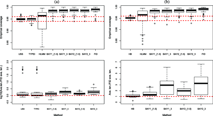
Figure 1: Summary of simulation results. (a) Displays the combined results for $\sigma_{\alpha}^{2}$ and $\sigma_{\beta}^{2}$ for the two-fold nested model. (b) Displays the combined results for $\sigma_{\alpha}^{2}$, $\sigma_{\beta}^{2}$ and $\sigma_{\alpha\beta}^{2}$ for the two-factor crossed design with interaction. The first row is the empirical coverage probabilities for 95% two-sided confidence intervals. The second row, first column is the $\mathrm{log}_{10}$ of the average interval lengths divided by the average interval lengths of FID, and the second row, second column is the average interval lengths divided by the average interval lengths of FID. Each value used in a box plot corresponds to a particular model design and parameter combination for each nonerror variance component. The average interval lengths for HLMM were not included in the displayed results due to their excessive lengths. All the simulation results are available in the supplemental document [Cisewski and Hannig (2012)].

HLMM has empirical coverage below the stated level, and the overall longest average interval lengths. ${\mathrm{BAY1}_{1.5}}$, ${\mathrm{BAY1}_{3}}$, ${\mathrm{BAY2}_{1.5}}$ and ${\mathrm{BAY2}_{3}}$ tend to be conservative with the longest average interval lengths after HLMM. USS and TYPEI maintain the stated coverage well, and FID tends to be conservative. Even though FID is conservative, its average interval lengths are comparable or shorter than those of USS and TYPEI. However, the average interval lengths of USS and TYPEI for $\sigma_{\beta}^{2}$ are surprisingly wider than ${\mathrm{BAY1}_{1.5}}$, ${\mathrm{BAY1}_{3}}$, ${\mathrm{BAY2}_{1.5}}$, ${\mathrm{BAY2}_{3}}$ and FID for MI-1, as revealed in the plot of the average lengths in Figure 1(a). This is due to the model design; specifically, the derivation of the confidence intervals results in the degrees of freedom of 1 for the nested factor (calculated as $\sum_{i=1}^{I}J_{i}-I=1$). ${\mathrm{BAY1}_{1.5}}$, ${\mathrm{BAY1}_{3}}$, ${\mathrm{BAY2}_{1.5}}$, ${\mathrm{BAY2}_{3}}$ and FID do not appear to have this issue. Upper and lower one-sided confidence interval results for $\sigma_{\alpha}^{2}$ and $\sigma_{\beta}^{2}$ for USS and TYPEI tend to stay within the stated level of coverage, and ${\mathrm{BAY1}_{1.5}}$, ${\mathrm{BAY1}_{3}}$, ${\mathrm{BAY2}_{1.5}}$, ${\mathrm{BAY2}_{3}}$ and FID range from staying within the stated level of coverage to very conservative.

The proposed method, while maintaining conservative coverage, has average interval lengths that are competitive or better than the other methods used in this part of the study. The proposed method offers an easily generalizable framework and provides intervals for fixed effects and the error variance component, unlike the methods presented in Hernandez, Burdick and Birch (1992). While the conservative coverage for the Bayesian methods can be deemed acceptable, their average interval lengths tend to be wider than the proposed method.

3.1.1 Application 1

In addition to the simulation study, we consider the application of model (10) presented in Hernandez, Burdick and Birch (1992) concerning the blood pH of female mice offspring. Fifteen dams were mated with 2 or 3 sires, where each sire was only used for one dam (i.e., 37 sires were used in the experiment), and the purpose of the study was to determine if the variability in the blood pH of the female offspring is, in part, due to the variability in the mother. There is imbalance in the data due to the number of sires mated with each dam (2 or 3); also note the natural imbalance in the data resulting from the number of female offspring.

The 95% confidence intervals based on the real data are presented in Table 2. An example of the generalized fiducial distribution for $\sigma_{\alpha}^{2}$ is displayed in Figure 2. This highlights one of the advantages of the proposed method over classical methods (and shared with Bayesian methods), which is a distribution on the parameter space allowing for inferences similar to those made using Bayesian posterior distributions.

Table 2: Two-fold nested model: real data example

Var. comp.	Method	95% 2-sided CI	2-sided/ave. len.	Upper/lower
$\sigma_{\alpha}^{2}$	USS	(2.30, 28.56)	0.953$/$25.1	0.949$/$0.958
	TYPEI	(1.94, 26.23)	0.950$/$25.2	0.949$/$0.957
	${\mathrm{BAY1}_{1.5}}$	(1.73, 30.72)	0.955$/$29.2	0.948$/$0.959
	${\mathrm{BAY1}_{3}}$	(1.51, 30.21)	0.956$/$37.2	0.948$/$0.962
	${\mathrm{BAY2}_{1.5}}$	(1.56, 30.02)	0.955$/$27.3	0.948$/$0.960
	${\mathrm{BAY2}_{3}}$	(1.76, 30.04)	0.955$/$27.5	0.950$/$0.961
	FID	(1.53, 26.67)	0.947$/$24.5	0.958$/$0.947
$\sigma_{\beta}^{2}$	USS	(0.00, 11.56)	0.961$/$10.9	0.952$/$0.952
	TYPEI	(0.00, 11.26)	0.964$/$12.4	0.953$/$0.953
	${\mathrm{BAY1}_{1.5}}$	(0.17, 11.81)	0.976$/$11.2	0.956$/$0.994
	${\mathrm{BAY1}_{3}}$	(0.04, 12.55)	0.980$/$11.3	0.959$/$0.996
	${\mathrm{BAY2}_{1.5}}$	(0.01, 12.49)	0.982$/$11.3	0.958$/$0.994
	${\mathrm{BAY2}_{3}}$	(0.01, 11.92)	0.983$/$11.3	0.958$/$0.995
	FID	(0.19, 10.54)	0.974$/$10.7	0.951$/$0.986

[]Note: The 95% intervals are based on the actual data while the remaining information are the empirical results from 2000 independently generated data set using the REML estimates for each parameter. The results are the empirical coverage and average interval lengths of 95% confidence intervals.

In order to evaluate the empirical coverage of the proposed method, we perform a simulation study using the REML estimates for all the parameters ($\mu=44.92$, $\sigma_{\alpha}^{2}=8.90$, $\sigma_{\beta}^{2}=2.65$ and $\sigma_{\varepsilon}^{2}=24.81$). Simulating 2000 independent data sets with the noted parameter values, we find the empirical coverage using USS, TYPEI, ${\mathrm{BAY1}_{1.5}}$, ${\mathrm{BAY1}_{3}}$, ${\mathrm{BAY2}_{1.5}}$, ${\mathrm{BAY2}_{3}}$ and FID, and the average lengths of the two-sided intervals. The results of the simulation study are also found in Table 2.

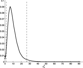
Figure 2: The generalized fiducial distribution of 5000 generated particles for $\sigma_{\alpha}^{2}$ using the real data described in Section 3.1.1. The solid line is the normal kernel density estimate of the distribution with a point mass at zero. The two vertical dashed lines represent the lower and upper bounds for 95% confidence intervals based on the weights of the generated particles.

The confidence interval coverage and average lengths for $\sigma_{\alpha}^{2}$ are comparable for all methods with ${\mathrm{BAY1}_{3}}$ having the longest average interval length. For $\sigma_{\beta}^{2}$, ${\mathrm{BAY1}_{1.5}}$, ${\mathrm{BAY1}_{3}}$, ${\mathrm{BAY2}_{1.5}}$, ${\mathrm{BAY2}_{3}}$ and FID tend to be more conservative while USS and TYPEI correctly maintain the stated level of coverage. USS, TYPEI and FID have comparable interval lengths, and the average lengths of ${\mathrm{BAY1}_{1.5}}$, ${\mathrm{BAY1}_{3}}$, ${\mathrm{BAY2}_{1.5}}$, ${\mathrm{BAY2}_{3}}$ are slightly longer.

3.2 Unbalanced two-factor crossed design with interaction

In this part of the simulation study, we consider the unbalanced two-factor crossed designs with interaction written as

$$Y_{ijk}=\mu+\alpha_{i}+\beta_{j}+(\alpha\beta)_{ij}+\varepsilon_{ijk}$$ (11)

for $i=1,\ldots,I$, $j=1,\ldots,J$ and $k=1,\ldots,K_{ij}$, where $\mu$ is an unknown constant and $\alpha_{i}\sim N(0,\sigma_{\alpha}^{2})$, $\beta_{j}\sim N(0,\sigma_{\beta}^{2})$, $(\alpha\beta)_{ij}\sim N(0,\sigma_{\alpha\beta}^{2})$ and $\varepsilon_{ijk}\sim N(0,\sigma_{\varepsilon}^{2})$.

This model is presented in Hernandez and Burdick (1993), where the authors propose a method based on unweighted sum of squares to construct confidence intervals for $\sigma_{\alpha}^{2}$, $\sigma_{\beta}^{2}$ and $\sigma_{\alpha\beta}^{2}$. The method they propose is based on intervals for balanced designs presented by Ting et al. (1990). In the simulation study, this method will be called HB. As with (10), HLMM from Lee and Nelder (1996), and ${\mathrm{BAY1}_{1.5}}$, ${\mathrm{BAY1}_{3}}$, ${\mathrm{BAY2}_{1.5}}$ and ${\mathrm{BAY2}_{3}}$ from Gelman (2006) will be used as a comparison.

Table 3 displays the model designs used in this part of the study, and, again, the overall measure of imbalance ($\phi$) proposed in Khuri (1987) is displayed for each design. The parameters values used in this part of the study are $\mu=0$, and the following combinations of $(\sigma_{\alpha}^{2},\sigma_{\beta}^{2},\sigma_{\alpha\beta}^{2},\sigma_{\varepsilon}^{2})$: $\mbox{PII-1}=(0.1,0.5,0.1,0.3)$, $\mbox{PII-2}=(0.1,0.3,0.1,0.5)$, $\mbox{PII-3}=(0.1,0.1,0.3,0.5)$, $\mbox{PII-4}=(0.1,0.1,0.5,0.3)$, and $\mbox{PII-5}=(1,1,1,1)$.

Table 3: Model designs used in the two-factor crossed design with interaction model of (11)

Design	$\bolds{\phi}$	$\bolds{I}$	$\bolds{J}$	$\bolds{K_{ij}}$	$\bolds{n}$
MII-1	$0.8768$	4	3	$2,1,3/2,1,1/2,2,2/1,2,3$	22
MII-2	$0.6667$	3	3	$4,1,1/4,1,1/4,1,1$	18
MII-3	$0.6667$	3	3	$4,4,4/1,1,1/1,1,1$	18
MII-4	$0.4011$	3	4	$8,1,1,1/1,1,1,1/1,1,1,1$	19
MII-5	$0.7619$	5	3	$1,2,2/5,2,7/2,2,2/2,4,2/3,2,2$	40
MII-6	$1.000$	3	3	$2,2,2/2,2,2/2,2,2$	18

[]Note: The parameter $\phi$ is an overall measure of imbalance of the model. See (11) for definitions of $I$, $J$ and $K_{ij}$; note sample size $(n)=\sum_{i}\sum_{j}K_{ij}$.

For each design and set of parameter values, 2000 independent data sets were generated, and 5000 particles were simulated for the proposed method. As before, performance is based on the empirical coverage of $(1-\alpha)100\%$ confidence intervals and average interval length for the parameter of interest $\theta$. Based on the normal approximation to the binomial distribution, we will consider empirical coverage between $94\%$ and $96\%$ appropriate for 95% two-sided confidence intervals.

A summary of the two-sided 95% confidence interval results for $\sigma_{\alpha}^{2}$, $\sigma_{\beta}^{2}$ and $\sigma_{\alpha\beta}^{2}$ are displayed in Figure 1. In addition, the supplemental document [Cisewski and Hannig (2012)] includes figures with the results summarized by parameter along with the complete raw data results. Average interval lengths are not included in the displayed results for HLMM because the excessive lengths would skew the scale of the plots; however, the average lengths are displayed in the raw data results in the supplemental document [Cisewski and Hannig (2012)].

HLMM has empirical coverage below the stated level, and the longest average interval lengths. While HB maintains the stated coverage and FID tends to be more conservative, they have comparable average interval lengths. ${\mathrm{BAY1}_{1.5}}$, ${\mathrm{BAY1}_{3}}$, ${\mathrm{BAY2}_{1.5}}$, and ${\mathrm{BAY2}_{3}}$ are conservative with the longest average interval lengths after HLMM for $\sigma_{\alpha}^{2}$ and $\sigma_{\beta}^{2}$; while still conservative for $\sigma_{\alpha\beta}^{2}$, the average interval lengths are shorter than HB, but longer than FID. One-sided confidence interval results for HB maintains the stated coverage, and ${\mathrm{BAY1}_{1.5}}$, ${\mathrm{BAY1}_{3}}$, ${\mathrm{BAY2}_{1.5}}$, ${\mathrm{BAY2}_{3}}$ and FID tends to be within the stated coverage to very conservative.

4 Conclusion

Even with the long history of inference procedures for normal linear mixed models, a good-performing, unified inference method is lacking. ANOVA-based methods offer, what tend to be, model-specific solutions. While Bayesian methods allow for solutions to very complex models, determining an appropriate prior distribution can be confusing for the nonstatistician practitioner. In addition, for the models considered in the simulation study and the prior selected based on recommendations in the literature, the Bayesian interval lengths were not generally competitive with the other methods used in the study. The proposed method allows for confidence interval estimation for all parameters of balanced and unbalanced normal linear mixed models. In general, our recommendation is to use the proposed method because of its apparent robustness to design imbalance, good small sample properties and flexibility of inference due to a fiducial distribution on the parameter space. If the design is balanced and only confidence intervals are desired, an ANOVA-based method would provide a computationally efficient solution.

It is interesting to note that even though more variation was incorporated into the data for the proposed method due to its acknowledgment of known uncertainty using intervals, in the simulation study, the proposed method tended to have conservative coverage, but the average interval lengths were comparable or shorter than the other methods that assumed the data are observed exactly. The currently implemented algorithm is suitable for 9 or fewer total parameters, but the method does not limit the number of parameters. A MATLAB implementation of the proposed algorithm is available on the author’s website at http://www.unc.edu/~hannig/download/ LinearMixedModel_MATLAB.zip.

Appendix A Resampling alteration step

The particle to be resampled is decomposed into an orthogonal projection onto a certain space (discussed below) and the part orthogonal to that space, and then the distributional properties that arise from the decomposition are used to alter the resampled particle. The alteration step of the proposed algorithm is performed in such a way that it still solves the system of inequalities of (5) up to time $t$ using the following idea (to ease the notational complexity, we do not include the dependence of the variables on $t$). Suppose particle $L$ is selected to be resampled (for an $L$ between 1 and $N$). For each random effect, $e$, let $Y={\mathbf{X}}^{\prime}{\beta}^{\prime}+\sigma{\mathbf{V}}Z^{(L)}$, where ${\mathbf{X}}^{\prime}=[\mathbf{X},\{\sum_{j=1}^{l_{i}}V_{i,j}z_{i,j}^{(L)}\}_{i\neq e}]$, $\beta^{\prime}=(\beta,\{\sigma_{i}\}_{i\neq e})^{\prime}$, $\sigma=\sigma_{e}$ and ${\mathbf{V}}Z^{(L)}=\sum_{j=1}^{l_{e}}V_{e,j}Z_{e,j}^{(L)}$. In order to alter $Z^{(L)}$, we first find the basis vectors, $\eta$, for the null space $\mathcal{N}=\operatorname{null}[-{\mathbf{X}}^{\prime},{\mathbf{V}}]={\eta}$ where for matrix ${\mathbf{A}}=[-{\mathbf{X}}^{\prime},{\mathbf{V}}]$, $\operatorname{null}({\mathbf{A}})$ is the set $\{\eta\dvtx{\mathbf{A}}\eta={\mathbf{0}}\}$, and ${\eta}=({\eta}_{1},{\eta}_{2})^{T}$ such that (i) ${\mathbf{X}}^{\prime}\cdot{\eta}_{1}={\mathbf{0}}$, (ii) ${\mathbf{V}}\cdot{\eta}_{2}={\mathbf{0}}$, (iii) ${\eta}_{2}^{T}\cdot{\eta}_{2}={\mathbf{I}}$ (i.e., ${\eta}_{2}$ is orthonormal) and (iv) $\operatorname{rank}(\eta)=\operatorname{rank}(\eta_{2})$. We perform the following decomposition:

$$Z^{(L)}=\Pi Z^{(L)}+\bigl{\|}Z^{(L)}-\Pi Z^{(L)}\bigr{\|}\cdot\frac{Z^{(L)}-\Pi Z^{(L)}}{\|Z^{(L)}-\Pi Z^{(L)}\|},$$ (12)

where $\Pi Z^{(L)}$ is the projection onto the null space $\mathcal{N}$ (i.e., $\Pi Z^{(L)}=\eta\cdot\eta^{T}\cdot Z^{(L)}$), and $\|\cdot\|$ is the $L^{2}$ norm. Define ${\mathbf{C}}=\eta_{2}^{T}\cdot Z^{(L)}$ (so that, $\eta_{2}\cdot{\mathbf{C}}=\Pi Z^{(L)}$), ${\mathbf{D}}=\|Z^{(L)}-\Pi Z^{(L)}\|$, and $\tau=\frac{Z^{(L)}-\Pi Z^{(L)}}{\|Z^{(L)}-\Pi Z^{(L)}\|}$. Then if $Z^{(L)}$ is standard normal, ${\mathbf{C}}\sim N_{l_{e}}(0,{\mathbf{I}})$ where $l_{e}$ is the number of levels of random effect $e$ of $Z^{(L)}$ to be resampled at time $t$, and ${\mathbf{D}}\sim\sqrt{\chi^{2}_{t-d}}$ where $d=\operatorname{rank}(\mathcal{N})$, and $\mathbf{C}$ and $\mathbf{D}$ are independent by design. The alteration of $Z^{(L)}$ is accomplished by sampling new values of ${\mathbf{C}}$ and ${\mathbf{D}}$ (denoted $\widetilde{{\mathbf{C}}}$ and $\widetilde{{\mathbf{D}}}$, resp.) according to their distributions determined by the decomposition above, and the altered particle is

$$\widetilde{Z}=\eta_{2}\cdot\widetilde{{\mathbf{C}}}+\widetilde{{\mathbf{D}}}\cdot\tau.$$ (13)

Notice that if $Z^{(L)}$ is a standard normal conditioned on $\mathbf{C}_{t}$, then so is $\widetilde{Z}$, and hence the alteration proposed still targets the correct distribution and is a Markovian step.

Furthermore, the set $Q_{t}^{(L)}=\{(\beta^{\prime},\sigma)\dvtx a_{i}<{\mathbf{X}}^{\prime}{\beta^{\prime}}+\sigma{\mathbf{V}}Z^{(L)}\leq b_{i},i=1,\ldots,t\}$ can be adjusted noting that if $(\beta^{\prime},\sigma)$ solves $a_{i}<{\mathbf{X}}^{\prime}\beta^{\prime}+\sigma{\mathbf{V}}(\eta_{2}\cdot{\mathbf{C}}+{\mathbf{D}}\cdot{\tau})\leq b_{i}$ for $i=1,\ldots,t$, then $(\widetilde{\beta},\widetilde{\sigma})$ can be found such that $a_{i}<{\mathbf{X}}^{\prime}\widetilde{\beta}+\widetilde{\sigma}{\mathbf{V}}(\eta_{2}\cdot\widetilde{\mathbf{C}}+\widetilde{\mathbf{D}}\cdot{\tau})\leq b_{i}$ for $i=1,\ldots,t$ by considering $\mathbf{X}^{\prime}\beta+\sigma\mathbf{V}Z=\mathbf{X}\beta+\sigma\mathbf{V}(\eta_{2}\cdot\mathbf{C}+\tau\mathbf{D})=\mathbf{X}^{\prime}\widetilde{\beta}+\widetilde{\sigma}\mathbf{V}(\eta_{2}\cdot\widetilde{\mathbf{C}}+\tau\widetilde{\mathbf{D}})=\mathbf{X}^{\prime}\widetilde{\beta}+\widetilde{\sigma}\mathbf{V}\widetilde{Z}$. Examining the orthogonal parts first, $\sigma\mathbf{V}(\tau\mathbf{D})=\widetilde{\sigma}\mathbf{V}(\tau\widetilde{\mathbf{D}})\mbox{ implies }\mathbf{V}\tau(\sigma\mathbf{D}-\widetilde{\sigma}\widetilde{\mathbf{D}})=0$ implies $\widetilde{\sigma}=\sigma(\mathbf{D}/\widetilde{\mathbf{D}})$. The relation between $\widetilde{\beta}$ and $\beta^{\prime}$ follows from the remaining portion

$$\displaystyle\mathbf{X}^{\prime}\beta^{\prime}+\sigma\mathbf{V}(\eta_{2}\cdot\mathbf{C})=\mathbf{X}^{\prime}\widetilde{\beta}+\widetilde{\sigma}\mathbf{V}(\eta_{2}\cdot\widetilde{\mathbf{C}})\quad\mbox{implies}$$

(14)

$$\displaystyle\mathbf{X}^{\prime}\bigl{(}\widetilde{\beta}-\beta^{\prime}\bigr{)}+\sigma\mathbf{V}\eta_{2}(\widetilde{\mathbf{C}}\cdot\mathbf{D}/\widetilde{\mathbf{D}}-\mathbf{C})=0.$$

Noting by definition $-\mathbf{X}^{\prime}\eta_{1}+\mathbf{V}\eta_{2}=0$, then

$$-\mathbf{X}^{\prime}\sigma\eta_{1}(\widetilde{\mathbf{C}}\cdot\mathbf{D}/\widetilde{\mathbf{D}}-\mathbf{C})+\sigma\mathbf{V}\eta_{2}(\widetilde{\mathbf{C}}\cdot\mathbf{D}/\widetilde{\mathbf{D}}-\mathbf{C})=0.$$ (15)

By combining (A) and (15), we see that $\widetilde{\beta}-\beta^{\prime}=-\sigma\eta_{1}\cdot(\widetilde{\mathbf{C}}\cdot\mathbf{D}/\widetilde{\mathbf{D}}-\mathbf{C})$, and hence $\widetilde{\beta}=\beta^{\prime}-\sigma\eta_{1}\cdot(\widetilde{\mathbf{C}}\cdot\mathbf{D}/\widetilde{\mathbf{D}}-\mathbf{C})$. Hence the sets $Q_{t}^{(J)}(Z_{1:t}^{(J)})$ are easily updated to $Q_{t}^{(J)}(\widetilde{Z}_{1:t}^{(J)})$. This procedure is repeated for each random effect.

Appendix B Prior distribution selection

The R package “rjags” was used to implement the Bayesian methods used in the simulation study and applications. Gelman (2006) suggests using a uniform prior [i.e., $U(0,a)$] on the standard deviation parameters when there are at least 5 groups and explains that fewer than 3 groups results in an improper posterior distribution. Calibration is necessary in selecting the parameter $a$ in the prior distribution; we use 1.5 and 3 times the range of the data (per the recommendation in Gelman [(2006), page 528] to use a value that is “high but not off the scale”), which appears reasonable when reviewing the resulting posterior distributions. In the simulation study, the results at these scale are denoted by ${\mathrm{BAY1}_{1.5}}$ and ${\mathrm{BAY1}_{3}}$, respectively. For example, the hierarchical model for the two-fold nested model of (10) is

$$Y_{ijk} \sim N\bigl{(}\mu+\alpha_{i}+\beta_{ij},\sigma_{\varepsilon}^{2}\bigr{)},\qquad i=1,\ldots,I,j=1,\ldots,J_{i},k=1,\ldots,K_{ij},$$

$$\alpha_{i} \sim N(0,\sigma_{\alpha}),\qquad i=1,\ldots,I,\qquad\beta_{ij}\sim N(0,\sigma_{\beta}),\qquad j=1,\ldots,J_{i},$$

$$\sigma_{\alpha} \sim U(0,a),\qquad\sigma_{\beta}\sim U(0,a).$$

For the second Bayesian method, a similar hierarchical model is used. Instead of a uniform distribution on the nonerror variance components, a half-Cauchy distribution with scale parameter $a$ set as 1.5 or 3 times the range of the data (denoted ${\mathrm{BAY2}_{1.5}}$ and ${\mathrm{BAY2}_{3}}$, resp., in the simulation study) is used.

Appendix C Proof of theorem

The proof of the convergence of the proposed SMC algorithm follows from ideas presented in Douc and Moulines (2008). Theorem 2.1 will follow from proving the convergence of the generated particles after each stage of the algorithm: sampling, resampling and alteration. The development of the particle system using the proposed algorithm does not follow the traditional SMC algorithm as presented in Douc and Moulines (2008), Section 2. A distinction is seen in the formulation of the proposed weights introduced in (9) and discussed below.

Using the derivation of the proposal distribution in and above (8), the target distribution of (7) and noting that $\mathbf{I}_{\mathbf{C}_{t}}(Z_{1:t})=\mathbf{I}_{\mathbf{C}_{t-1}}(Z_{1:t-1})\cdot\mathbf{I}_{\star}(Z_{t,1:r-1})\cdot\mathbf{I}_{(m_{t}(Z_{1:t-1},Z_{t,1:r-1}),M_{t}(Z_{1:t-1},Z_{t,1:r-1}))}(z_{t,r})$ [where the $\star$ in$\mathbf{I}_{\star}(Z_{t,1:r-1})$ indicates the lack of restriction to a specific set of values for $Z_{t,1:r-1}$], the marginal target distribution at time $t$ is

$$\widehat{\pi}_{1:t-1} = \int\pi_{1:t}(Z_{1:t})\,dZ_{t}=\int\frac{\exp(-(Z_{1:t}^{T}\cdot Z_{1:t})/2){\mathbf{I}_{\mathbf{C}_{t}}}(Z_{1:t})}{\Theta_{1:t}}\,dZ_{t}$$

$$\propto \pi_{1:t-1}\int\exp\bigl{(}-\bigl{(}Z_{t}^{T}\cdot Z_{t}\bigr{)}/2\bigr{)}$$

$$\hskip 38.0pt{}\times\mathbf{I}_{\star}(Z_{t,1:r-1})\mathbf{I}_{(m_{t}(Z_{1:t-1},Z_{t,1:r-1}),M_{t}(Z_{1:t-1},Z_{t,1:r-1}))}(z_{t,r})\,dZ_{t}$$

$$\propto \pi_{1:t-1}\cdot\bigl{(}\Phi\bigl{(}M_{t}(Z_{1:t-1},Z_{t,1:r-1})\bigr{)}-\Phi\bigl{(}m_{t}(Z_{1:t-1},Z_{t,1:r-1})\bigr{)}\bigr{)},$$

where $F$ and $\Phi$ are the standard Cauchy and standard normal cumulative distribution functions, respectively, and $\Theta_{1:t}$ is the normalization factor at time $t$. It then follows that the conditional target distribution at time $t$ is

$$\pi_{t|1:t-1}$$

$$\qquad=\pi_{1:t}(Z_{1:t})/\widehat{\pi}_{1:t}(Z_{1:t})$$

$$\qquad\propto{\exp\bigl{(}-(Z_{t}^{T}\cdot Z_{t})/2\bigr{)}\cdot\mathbf{I}_{\star}(Z_{t,1:r-1})\cdot\mathbf{I}_{(m_{t}(Z_{1:t-1},Z_{t,1:r-1}),M_{t}(Z_{1:t-1},\mathbf{Z}_{t,1:r-1}))}(z_{t,r})}$$

$$\qquad\quad{}/\bigl{(}{\Phi\bigl{(}M_{t}(Z_{1:t-1},Z_{t,1:r-1})\bigr{)}-\Phi\bigl{(}m_{t}(Z_{1:t-1},Z_{t,1:r-1})\bigr{)}}\bigr{)}.$$

Finally, following the notation just below (9), the derivation of the weights at time $t$ is $W_{1:t}=\frac{\pi_{1:t}}{\widetilde{\pi}_{1:t}}=\frac{\pi_{t|1:t-1}\cdot\widehat{\pi}_{1:t-1}}{\widetilde{\pi}_{t|1:t-1}\cdot\widetilde{\pi}_{1:t-1}}\propto\exp(-z_{t,r}^{2}/2)(1+z_{t,r}^{2})(F(M_{t}(Z_{1:t-1}$, $Z_{t,1:r-1}))-F(m_{t}(Z_{1:t-1},Z_{t,1:r-1})))\cdot\frac{\pi_{1:t-1}}{\widetilde{\pi}_{1:t-1}}\propto W_{t}\cdot W_{1:t-1}$. This proof will use the above formulation and the following notation and definition.

A particle system is defined as $\{Z_{1:t}^{(J)},W_{1:t}^{(J)}\}_{J=1}^{N}$ with $Z_{1:t}^{(J)}$ sampled from the proposal distribution $\widetilde{\pi}_{1:t}$ as defined in (8) targeting probability measure $\pi_{1:t}$ on $(\Theta_{1:t},\mathcal{B}(\Theta_{1:t}))$, and un-normalized weights $W_{1:t}^{(J)}$ as defined in (9). Let $\widetilde{\pi}_{t|1:t-1}$ be the marginal proposal density at time $t$ as defined above equation (8), which follows a Cauchy distribution truncated to the region $R_{t}\triangleq(m_{t}(Z_{1:t-1},Z_{t,1:r-1}),M_{t}(Z_{1:t-1},Z_{t,1:r-1}))$ defined by previously sampled particles. For notational convenience, let $\Omega_{t}=\sum_{J=1}^{N}W_{1:t}^{(J)}$. Define two sigma-fields $\mathcal{F}_{0}\triangleq\sigma(\{Z_{1:t}^{(J)}\}_{J=1}^{N},(a,b]_{1:t})$ and $\widetilde{\mathcal{F}}_{J}\triangleq\mathcal{F}_{0}\vee\sigma(\{\widetilde{Z}_{1:t}^{(K)}\}_{1\leq K\leq J},\break(a,b]_{1:t})$, for $J=1,\ldots,N$. Finally, we define proper set $B_{t}$ [Douc and Moulines (2008), Section 2.1] where $B_{t}\triangleq\{f\in L^{1}(\Theta_{1:t},\pi_{1:t}),F(\cdot,|f|)\in B_{t-1}\}$ and$F(Z_{1:t-1},f)=\int f(Z_{1:t-1},Z_{t})\mathbf{I}_{\star}(Z_{t,1:r-1})\mathbf{I}_{R_{t}}(z_{t,r})(\Phi(M_{t}(Z_{1:t-1},Z_{t,1:r-1}))-\break\Phi(m_{t}(Z_{1:t-1},Z_{t,1:r-1})))\pi_{t|1:t-1}(dZ_{t})$.

Definition C.1.

Following Definition 1 of Douc and Moulines (2008), a weighted sample $\{Z_{1:t}^{(J)},W_{1:t}^{(J)}\}_{J=1,\ldots,N}$ is consistent for the probability measure $\pi_{1:t}$ and the proper set $B_{t}$ if, for any $f\in B_{t}$, $\Omega_{t}^{-1}\sum_{J=1}^{N}W_{1:t}^{(J)}f(Z_{1:t}^{(J)})\stackrel{{\scriptstyle P}}{{\longrightarrow}}\int f(Z_{1:t})\pi_{1:t}(dZ_{1:t})\triangleq\pi_{1:t}(f)$, and $\Omega_{t}^{-1}\max_{J=1}^{N}W_{1:t}^{(J)}\stackrel{{\scriptstyle P}}{{\longrightarrow}}0$.

Two additional conditions on the set $B_{t}$ will be required to guarantee consistency for the particle system after the alteration step. Let $f\in B_{t}$, and $\Pi$ be the projection matrix onto the null space defined in the description of the resampling step of the algorithm found in Appendix A. $E[f(\widetilde{Z}_{1:t}^{(J)})\mid\mathcal{\widetilde{F}}_{J-1}]=\int f(\eta_{2}\cdot\widetilde{C}+\widetilde{D}\frac{(Z_{1:t}^{(J)}-\Pi Z_{1:t}^{(J)})}{\|Z_{1:t}^{(J)}-\Pi Z_{1:t}^{(J)}\|})\,d\pi_{\widetilde{C},\widetilde{D}}=\int f(\eta_{2}\cdot\widetilde{C}+\widetilde{D}\tau_{1:t}^{(J)})\,d\pi_{\widetilde{C},\widetilde{D}}\triangleq h_{f}(Z_{1:t}^{(J)})$, where $\widetilde{C}$ and $\widetilde{D}$ are as defined above (13). For $h_{f}$ to be in $B_{t}$, $f$ must be selected so that the following two conditions hold for any direction $\tau_{1:t}$:

$$\int\bigl{|}h_{f}(\widetilde{Z}_{1:t})\bigr{|}\,d\pi_{1:t} = \int\biggl{|}\int f(\eta_{2}\cdot\widetilde{C}+\widetilde{D}\tau_{1:t})\,d\pi_{\widetilde{C},\widetilde{D}}\biggr{|}\,d\pi_{1:t}<\infty,$$ (16)

$$F(\widetilde{Z}_{1:t-1},h_{f}) = \int\biggl{(}\int f\bigl{(}\eta_{2}\cdot\widetilde{C}+\widetilde{D}\tau_{1:t}^{\prime}\bigr{)}\,d\pi_{\widetilde{C},\widetilde{D}}\biggr{)}\cdot\mathbf{I}_{C_{t}}(Z_{1:t})$$

$$\hskip 7.3pt{}\times\bigl{(}\Phi(M_{t})-\Phi(m_{t})\bigr{)}\pi_{t\mid 1:t-1}(dZ_{t})<\infty,$$

where $\tau_{1:t}^{\prime}=\frac{([Z_{1:t-1},Z_{t}]-\Pi[Z_{1:t-1},Z_{t}])}{\|[Z_{1:t-1},Z_{t}]-\Pi[Z_{1:t-1},Z_{t}]\|}$. Let $\widetilde{B}_{t}$ be the set of $f\in B_{t}$ such that (16) and (C) hold. Then, $\widetilde{B}_{t}\subset B_{t}$, and we replace $B_{t}$ with $\widetilde{B}_{t}$ in the definition of $B_{t+1}$. Finally, since all bounded functions satisfy (16) and (C), $\widetilde{B}_{t}$ is nonempty.

The goal is to show the particle system generated from the presented algorithm is consistent. This requires the particle system after sampling and reweighting to be consistent, after resampling to be consistent and after the alteration to be consistent.

After noting (i) for $f\in B_{t}$, $E(W_{1:t}^{(J)}f(Z_{1:t}^{(J)})\mid\mathcal{F}_{J-1})=W_{1:t-1}^{(J)}E(W_{t}^{(J)}f(Z_{1:t}^{(J)})\mid\mathcal{F}_{J-1})=W_{1:t-1}^{(J)}\cdot F(Z_{1:t-1},f)$ for $J=1,\ldots,N$, with $F$ is defined aboveand $\mathcal{F}_{J-1}\triangleq\sigma(\{Z_{1:t-1}^{(J)}\}_{J=1}^{N},(a,b]_{1:t})\vee\sigma(\{Z_{1:t}^{(K)}\}_{1\leq K\leq J-1},(a,b]_{1:t})$, and(ii) $W_{t}\widetilde{\pi}_{t\mid 1:t-1}=(\Phi(M_{t})-\Phi(m_{t}))\pi_{t|1:t-1}$, consistency after sampling and reweighting closely follows the proof of Theorem 1 in Douc and Moulines (2008). Consistency after resampling follows directly from Theorem 3 in Douc and Moulines (2008) and consistency after the alteration step is addressed below in Lemma C.1.

Lemma C.1 ((Alteration))

Assuming the uniformly weighted sample$\{Z_{1:t}^{(J)},1\}_{J=1}^{N}$ is consistent for $(\pi_{1:t},B_{t})$, then the altered uniformly weighted sample $\{\widetilde{Z}_{1:t}^{(J)},1\}_{J=1}^{N}$ is consistent for $(\pi_{1:t},\widetilde{B}_{t})$.

Note that the $\{\widetilde{Z}_{1:t}^{(J)},1\}_{J=1}^{N}$ is the altered particle system, while $\{Z_{1:t}^{(J)},1\}_{J=1}^{N}$ are the resampled particles. We note that $h_{f}$ is a function of $Z_{1:t}$ because $\tau_{1:t}$ is a function of $Z_{1:t}$, and, at times, it will be necessary to write $\tau_{1:t}^{(J)}=\tau_{1:t}(Z_{1:t}^{(J)}$). Recall that $C$ and $D$ are defined by a decomposition of the original particle selected to be resampled and are independent by design. The $\widetilde{C}$ and $\widetilde{D}$ are the random variables to be resampled according to the target distributions of $C$ and $D$ with the $\tau_{1:t}^{(J)}$ considered fixed so that $\widetilde{Z}_{1:t}=\eta_{2}\cdot\widetilde{C}+\widetilde{D}\tau_{1:t}$.

The lemma will follow once we show

$$N^{-1}\sum_{J=1}^{N}E\bigl{[}f\bigl{(}\widetilde{Z}_{1:t}^{(J)}\bigr{)}\mid\mathcal{\widetilde{F}}_{J-1}\bigr{]}=N^{-1}\sum_{J=1}^{N}h_{f}\bigl{(}Z_{1:t}^{(J)}\bigr{)}$$

$$\quad\longrightarrow\quad\int h_{f}(Z_{1:t})\pi_{1:t}(dZ_{1:t})=\int f(Z_{1:t})\pi_{1:t}(dZ_{1:t}).$$

This is because trivially $E[f(\widetilde{Z}_{1:t}^{(J)})\mid\mathcal{\widetilde{F}}_{J-1}]=f(\widetilde{Z}_{1:t}^{(J)})$, so all that is needed is for:

i(i) $N^{-1}\sum_{J=1}^{N}h_{f}(Z_{1:t}^{(J)})\longrightarrow\int h_{f}(Z_{1:t})\pi_{1:t}(dZ_{1:t})$ and

(ii) $\int h_{f}(Z_{1:t})\,d\pi_{1:t}(Z_{1:t})=\int f(Z_{1:t})\pi_{1:t}(dZ_{1:t})$.

Point (i) follows from (16), (C), and because $f\!\in\!\widetilde{B}_{t}$ so that $h_{f}\!\in\!B_{t}$. Now we only need to show point (ii) that $\int h_{f}(Z_{1:t})\pi_{1:t}(dZ_{1:t})=\int f(Z_{1:t})\pi_{1:t}(dZ_{1:t})$. This holds because

$$\int h_{f}(Z_{1:t})\,d\pi_{1:t} = \int h_{f}^{*}(\tau_{1:t})\,d\pi_{\tau}$$

$$= \int\biggl{(}\int f(\eta_{2}\cdot\widetilde{C}+\widetilde{D}\tau_{1:t})\,d\pi_{\widetilde{C},\widetilde{D}}\biggr{)}\,d\pi_{\tau}$$

$$= \int\biggl{(}\int f(\eta_{2}\cdot C+D\tau_{1:t})\,d\pi_{C,D}\biggr{)}\,d\pi_{\tau}$$

$$= \int f(\eta_{2}\cdot C+D\tau_{1:t})\,d\pi_{C,D}\times d\pi_{\tau}$$

$$= \int f(Z_{1:t})\,d\pi_{1:t}=E_{\pi_{1:t}}\bigl{[}f(Z_{1:t})\bigr{]},$$

where $h_{f}^{*}(\tau_{1:t})=h_{f}(Z_{1:t})$, the equality from line one to line three follows because $\tau(Z_{1:t})=\tau(\widetilde{Z}_{1:t})$ and the equality in the third and fourth lines follows by Fubini’s theorem because $\widetilde{C}$ and $\widetilde{D}$ are independent of $\tau$.

References

- Burch (2011) {barticle}[mr] \bauthor\bsnmBurch, \bfnmBrent D.\binitsB. D. (\byear2011). \btitleAssessing the performance of normal-based and REML-based confidence intervals for the intraclass correlation coefficient. \bjournalComput. Statist. Data Anal. \bvolume55 \bpages1018–1028. \biddoi=10.1016/j.csda.2010.08.007, issn=0167-9473, mr=2736490 \bptokimsref \endbibitem
- Burch and Iyer (1997) {barticle}[mr] \bauthor\bsnmBurch, \bfnmBrent D.\binitsB. D. and \bauthor\bsnmIyer, \bfnmHari K.\binitsH. K. (\byear1997). \btitleExact confidence intervals for a variance ratio (or heritability) in a mixed linear model. \bjournalBiometrics \bvolume53 \bpages1318–1333. \biddoi=10.2307/2533500, issn=0006-341X, mr=1614382 \bptokimsref \endbibitem
- Burdick and Graybill (1992) {bbook}[mr] \bauthor\bsnmBurdick, \bfnmRichard K.\binitsR. K. and \bauthor\bsnmGraybill, \bfnmFranklin A.\binitsF. A. (\byear1992). \btitleConfidence Intervals on Variance Components. \bseriesStatistics: Textbooks and Monographs \bvolume127. \bpublisherDekker, \blocationNew York. \bidmr=1192783 \bptokimsref \endbibitem
- Casella and Berger (2002) {bbook}[author] \bauthor\bsnmCasella, \bfnmGeorge\binitsG. and \bauthor\bsnmBerger, \bfnmRoger L.\binitsR. L. (\byear2002). \btitleStatistical Inference, \bedition2nd ed. \bpublisherWadsworth and Brooks/Cole Advanced Books and Software, \blocationPacific Grove, CA. \bidmr=1051420 \bptokimsref \endbibitem
- Chopin (2002) {barticle}[mr] \bauthor\bsnmChopin, \bfnmNicolas\binitsN. (\byear2002). \btitleA sequential particle filter method for static models. \bjournalBiometrika \bvolume89 \bpages539–551. \biddoi=10.1093/biomet/89.3.539, issn=0006-3444, mr=1929161 \bptokimsref \endbibitem
- Chopin (2004) {barticle}[mr] \bauthor\bsnmChopin, \bfnmNicolas\binitsN. (\byear2004). \btitleCentral limit theorem for sequential Monte Carlo methods and its application to Bayesian inference. \bjournalAnn. Statist. \bvolume32 \bpages2385–2411. \biddoi=10.1214/009053604000000698, issn=0090-5364, mr=2153989 \bptokimsref \endbibitem
- Cisewski and Hannig (2012) {bmisc}[author] \bauthor\bsnmCisewski, \bfnmJessi\binitsJ. and \bauthor\bsnmHannig, \bfnmJan\binitsJ. (\byear2012). \bhowpublishedSupplement to “Generalized fiducial inference for normal linear mixed models.” DOI:\doiurl10.1214/12-AOS1030SUPP. \bptokimsref \endbibitem
- Del Moral, Doucet and Jasra (2006) {barticle}[mr] \bauthor\bsnmDel Moral, \bfnmPierre\binitsP., \bauthor\bsnmDoucet, \bfnmArnaud\binitsA. and \bauthor\bsnmJasra, \bfnmAjay\binitsA. (\byear2006). \btitleSequential Monte Carlo samplers. \bjournalJ. R. Stat. Soc. Ser. B Stat. Methodol. \bvolume68 \bpages411–436. \biddoi=10.1111/j.1467-9868.2006.00553.x, issn=1369-7412, mr=2278333 \bptokimsref \endbibitem
- Diaconis and Freedman (1986a) {barticle}[mr] \bauthor\bsnmDiaconis, \bfnmP.\binitsP. and \bauthor\bsnmFreedman, \bfnmD.\binitsD. (\byear1986a). \btitleOn inconsistent Bayes estimates of location. \bjournalAnn. Statist. \bvolume14 \bpages68–87. \biddoi=10.1214/aos/1176349843, issn=0090-5364, mr=0829556 \bptokimsref \endbibitem
- Diaconis and Freedman (1986b) {barticle}[mr] \bauthor\bsnmDiaconis, \bfnmPersi\binitsP. and \bauthor\bsnmFreedman, \bfnmDavid\binitsD. (\byear1986b). \btitleOn the consistency of Bayes estimates (with discussion). \bjournalAnn. Statist. \bvolume14 \bpages1–67. \biddoi=10.1214/aos/1176349830, issn=0090-5364, mr=0829555 \bptokimsref \endbibitem
- Douc, Cappé and Moulines (2005) {binproceedings}[author] \bauthor\bsnmDouc, \bfnmRandal\binitsR., \bauthor\bsnmCappé, \bfnmOlivier\binitsO. and \bauthor\bsnmMoulines, \bfnmEric\binitsE. (\byear2005). \btitleComparison of resampling schemes for particle filtering. In \bbooktitle4th International Symposium on Image and Signal Processing and Analysis \bpages64–69. \bptokimsref \endbibitem
- Douc and Moulines (2008) {barticle}[mr] \bauthor\bsnmDouc, \bfnmRandal\binitsR. and \bauthor\bsnmMoulines, \bfnmEric\binitsE. (\byear2008). \btitleLimit theorems for weighted samples with applications to sequential Monte Carlo methods. \bjournalAnn. Statist. \bvolume36 \bpages2344–2376. \biddoi=10.1214/07-AOS514, issn=0090-5364, mr=2458190 \bptokimsref \endbibitem
- Doucet, de Freitas and Gordon (2001) {bbook}[mr] \beditor\bsnmDoucet, \bfnmArnaud\binitsA., \beditor\bparticlede \bsnmFreitas, \bfnmNando\binitsN. and \beditor\bsnmGordon, \bfnmNeil\binitsN., eds. (\byear2001). \btitleSequential Monte Carlo Methods in Practice. \bpublisherSpringer, \blocationNew York. \bidmr=1847783 \bptokimsref \endbibitem
- E, Hannig and Iyer (2008) {barticle}[mr] \bauthor\bsnmE, \bfnmLidong\binitsL., \bauthor\bsnmHannig, \bfnmJan\binitsJ. and \bauthor\bsnmIyer, \bfnmHari\binitsH. (\byear2008). \btitleFiducial intervals for variance components in an unbalanced two-component normal mixed linear model. \bjournalJ. Amer. Statist. Assoc. \bvolume103 \bpages854–865. \biddoi=10.1198/016214508000000229, issn=0162-1459, mr=2524335 \bptokimsref \endbibitem
- Elster (2000) {barticle}[author] \bauthor\bsnmElster, \bfnmClemens\binitsC. (\byear2000). \btitleEvaluation of measurement uncertainty in the presence of combined random and analogue-to-digital conversion errors. \bjournalMeasurement Science and Technology \bvolume11 \bpages1359–1363. \bptokimsref \endbibitem
- Fisher (1930) {barticle}[author] \bauthor\bsnmFisher, \bfnmR. A.\binitsR. A. (\byear1930). \btitleInverse probability. \bjournalMath. Proc. Cambridge Philos. Soc. \bvolumexxvi \bpages528–535. \bptokimsref \endbibitem
- Fisher (1933) {barticle}[author] \bauthor\bsnmFisher, \bfnmR. A.\binitsR. A. (\byear1933). \btitleThe concepts of inverse probability and fiducial probability referring to unknown parameters. \bjournalProc. R. Soc. Lond. Ser. A \bvolume139 \bpages343–348. \bptokimsref \endbibitem
- Fisher (1935) {barticle}[author] \bauthor\bsnmFisher, \bfnmR. A.\binitsR. A. (\byear1935). \btitleThe fiducial argument in statistical inference. \bjournalAnnals of Eugenics \bvolumeVI \bpages91–98. \bptokimsref \endbibitem
- Fraser (1961a) {barticle}[mr] \bauthor\bsnmFraser, \bfnmD. A. S.\binitsD. A. S. (\byear1961a). \btitleThe fiducial method and invariance. \bjournalBiometrika \bvolume48 \bpages261–280. \bidissn=0006-3444, mr=0133910 \bptokimsref \endbibitem
- Fraser (1961b) {barticle}[mr] \bauthor\bsnmFraser, \bfnmD. A. S.\binitsD. A. S. (\byear1961b). \btitleOn fiducial inference. \bjournalAnn. Math. Statist. \bvolume32 \bpages661–676. \bidissn=0003-4851, mr=0130755 \bptokimsref \endbibitem
- Fraser (1966) {barticle}[mr] \bauthor\bsnmFraser, \bfnmD. A. S.\binitsD. A. S. (\byear1966). \btitleStructural probability and a generalization. \bjournalBiometrika \bvolume53 \bpages1–9. \bidissn=0006-3444, mr=0196840 \bptokimsref \endbibitem
- Fraser (1968) {bbook}[mr] \bauthor\bsnmFraser, \bfnmD. A. S.\binitsD. A. S. (\byear1968). \btitleThe Structure of Inference. \bpublisherWiley, \blocationNew York. \bidmr=0235643 \bptokimsref \endbibitem
- Frenkel and Kirkup (2005) {barticle}[author] \bauthor\bsnmFrenkel, \bfnmR. B.\binitsR. B. and \bauthor\bsnmKirkup, \bfnmL.\binitsL. (\byear2005). \btitleMonte Carlo-based estimation of uncertainty owing to limited resolution of digital instruments. \bjournalMetrologia \bvolume42 \bpagesL27–L30. \bptokimsref \endbibitem
- Gelman (2006) {barticle}[mr] \bauthor\bsnmGelman, \bfnmAndrew\binitsA. (\byear2006). \btitlePrior distributions for variance parameters in hierarchical models (comment on article by Browne and Draper). \bjournalBayesian Anal. \bvolume1 \bpages515–533 (electronic). \bidmr=2221284 \bptnotecheck related\bptokimsref \endbibitem
- Gelman et al. (2004) {bbook}[mr] \bauthor\bsnmGelman, \bfnmAndrew\binitsA., \bauthor\bsnmCarlin, \bfnmJohn B.\binitsJ. B., \bauthor\bsnmStern, \bfnmHal S.\binitsH. S. and \bauthor\bsnmRubin, \bfnmDonald B.\binitsD. B. (\byear2004). \btitleBayesian Data Analysis, \bedition2nd ed. \bpublisherChapman & Hall/CRC, \blocationBoca Raton, FL. \bidmr=2027492 \bptokimsref \endbibitem
- Ghosal, Ghosh and van der Vaart (2000) {barticle}[mr] \bauthor\bsnmGhosal, \bfnmSubhashis\binitsS., \bauthor\bsnmGhosh, \bfnmJayanta K.\binitsJ. K. and \bauthor\bparticlevan der \bsnmVaart, \bfnmAad W.\binitsA. W. (\byear2000). \btitleConvergence rates of posterior distributions. \bjournalAnn. Statist. \bvolume28 \bpages500–531. \biddoi=10.1214/aos/1016218228, issn=0090-5364, mr=1790007 \bptokimsref \endbibitem
- GUM (1995) {bmisc}[author] \borganizationGUM (\byear1995). \bhowpublishedGuide to the Expression of Uncertainty in Measurement. International Organization for Standardization (ISO), Geneva, Switzerland. \bptokimsref \endbibitem
- Hannig (2009) {barticle}[mr] \bauthor\bsnmHannig, \bfnmJan\binitsJ. (\byear2009). \btitleOn generalized fiducial inference. \bjournalStatist. Sinica \bvolume19 \bpages491–544. \bidissn=1017-0405, mr=2514173 \bptokimsref \endbibitem
- Hannig (2012) {bmisc}[author] \bauthor\bsnmHannig, \bfnmJ.\binitsJ. (\byear2012). \bhowpublishedGeneralized fiducial inference via discretizations. Statist. Sinica. To appear. \bptokimsref \endbibitem
- Hannig, Iyer and Patterson (2006) {barticle}[mr] \bauthor\bsnmHannig, \bfnmJan\binitsJ., \bauthor\bsnmIyer, \bfnmHari\binitsH. and \bauthor\bsnmPatterson, \bfnmPaul\binitsP. (\byear2006). \btitleFiducial generalized confidence intervals. \bjournalJ. Amer. Statist. Assoc. \bvolume101 \bpages254–269. \biddoi=10.1198/016214505000000736, issn=0162-1459, mr=2268043 \bptokimsref \endbibitem
- Hannig, Iyer and Wang (2007) {barticle}[author] \bauthor\bsnmHannig, \bfnmJan\binitsJ., \bauthor\bsnmIyer, \bfnmH. K.\binitsH. K. and \bauthor\bsnmWang, \bfnmJ. C. M.\binitsJ. C. M. (\byear2007). \btitleFiducial approach to uncertainty assessment: Accounting for error due to instrument resolution. \bjournalMetrologia \bvolume44 \bpages476–483. \bptokimsref \endbibitem
- Hannig and Lee (2009) {barticle}[mr] \bauthor\bsnmHannig, \bfnmJan\binitsJ. and \bauthor\bsnmLee, \bfnmThomas C. M.\binitsT. C. M. (\byear2009). \btitleGeneralized fiducial inference for wavelet regression. \bjournalBiometrika \bvolume96 \bpages847–860. \biddoi=10.1093/biomet/asp050, issn=0006-3444, mr=2767274 \bptokimsref \endbibitem
- Hartley and Rao (1967) {barticle}[mr] \bauthor\bsnmHartley, \bfnmH. O.\binitsH. O. and \bauthor\bsnmRao, \bfnmJ. N. K.\binitsJ. N. K. (\byear1967). \btitleMaximum-likelihood estimation for the mixed analysis of variance model. \bjournalBiometrika \bvolume54 \bpages93–108. \bidissn=0006-3444, mr=0216684 \bptokimsref \endbibitem
- Hernandez, Burdick and Birch (1992) {barticle}[author] \bauthor\bsnmHernandez, \bfnmRamon P.\binitsR. P., \bauthor\bsnmBurdick, \bfnmRichard K.\binitsR. K. and \bauthor\bsnmBirch, \bfnmNancy J.\binitsN. J. (\byear1992). \btitleConfidence intervals and tests of hypotheses on variance components in an unbalanced two-fold nested design. \bjournalBiom. J. \bvolume34 \bpages387–402. \bptokimsref \endbibitem
- Hernandez and Burdick (1993) {barticle}[author] \bauthor\bsnmHernandez, \bfnmRamon P.\binitsR. P. and \bauthor\bsnmBurdick, \bfnmRichard K.\binitsR. K. (\byear1993). \btitleConfidence intervals and tests of hypotheses on variance components in an unbalanced two-factor crossed design with interactions. \bjournalJ. Stat. Comput. Simul. \bvolume47 \bpages67–77. \bptokimsref \endbibitem
- Jasra, Stephens and Holmes (2007) {barticle}[mr] \bauthor\bsnmJasra, \bfnmAjay\binitsA., \bauthor\bsnmStephens, \bfnmDavid A.\binitsD. A. and \bauthor\bsnmHolmes, \bfnmChristopher C.\binitsC. C. (\byear2007). \btitleOn population-based simulation for static inference. \bjournalStat. Comput. \bvolume17 \bpages263–279. \biddoi=10.1007/s11222-007-9028-9, issn=0960-3174, mr=2405807 \bptokimsref \endbibitem
- Jeyaratnam and Graybill (1980) {barticle}[author] \bauthor\bsnmJeyaratnam, \bfnmS.\binitsS. and \bauthor\bsnmGraybill, \bfnmFranklin A.\binitsF. A. (\byear1980). \btitleConfidence intervals on variance components in three-factor cross-classification models. \bjournalTechnometrics \bvolume22 \bpages375–380. \bptokimsref \endbibitem
- Jiang (2007) {bbook}[mr] \bauthor\bsnmJiang, \bfnmJiming\binitsJ. (\byear2007). \btitleLinear and Generalized Linear Mixed Models and Their Applications. \bpublisherSpringer, \blocationNew York. \bidmr=2308058 \bptokimsref \endbibitem
- Khuri (1987) {barticle}[mr] \bauthor\bsnmKhuri, \bfnmA. I.\binitsA. I. (\byear1987). \btitleMeasures of imbalance for unbalanced models. \bjournalBiom. J. \bvolume29 \bpages383–396. \biddoi=10.1002/bimj.4710290402, issn=0323-3847, mr=0905958 \bptokimsref \endbibitem
- Khuri and Sahai (1985) {barticle}[mr] \bauthor\bsnmKhuri, \bfnmA. I.\binitsA. I. and \bauthor\bsnmSahai, \bfnmHardeo\binitsH. (\byear1985). \btitleVariance components analysis: A selective literature survey. \bjournalInternat. Statist. Rev. \bvolume53 \bpages279–300. \biddoi=10.2307/1402893, issn=0306-7734, mr=0967214 \bptokimsref \endbibitem
- Kong, Liu and Wong (1994) {barticle}[author] \bauthor\bsnmKong, \bfnmA.\binitsA., \bauthor\bsnmLiu, \bfnmJ. S.\binitsJ. S. and \bauthor\bsnmWong, \bfnmW. H.\binitsW. H. (\byear1994). \btitleSequential imputations and Bayesian missing data problems. \bjournalJ. Amer. Statist. Assoc. \bvolume89 \bpages278–288. \bptokimsref \endbibitem
- Laird and Ware (1982) {barticle}[author] \bauthor\bsnmLaird, \bfnmNan M.\binitsN. M. and \bauthor\bsnmWare, \bfnmJames H.\binitsJ. H. (\byear1982). \btitleRandom-effects models for longitudinal data. \bjournalBiometrics \bvolume38 \bpages963–974. \bptokimsref \endbibitem
- Le Cam (1986) {bbook}[mr] \bauthor\bsnmLe Cam, \bfnmLucien\binitsL. (\byear1986). \btitleAsymptotic Methods in Statistical Decision Theory. \bpublisherSpringer, \blocationNew York. \biddoi=10.1007/978-1-4612-4946-7, mr=0856411 \bptokimsref \endbibitem
- Lee and Nelder (1996) {barticle}[mr] \bauthor\bsnmLee, \bfnmY.\binitsY. and \bauthor\bsnmNelder, \bfnmJ. A.\binitsJ. A. (\byear1996). \btitleHierarchical generalized linear models. \bjournalJ. R. Stat. Soc. Ser. B Stat. Methodol. \bvolume58 \bpages619–678. \bidissn=0035-9246, mr=1410182 \bptnotecheck related\bptokimsref \endbibitem
- Lee, Nelder and Pawitan (2006) {bbook}[mr] \bauthor\bsnmLee, \bfnmYoungjo\binitsY., \bauthor\bsnmNelder, \bfnmJohn A.\binitsJ. A. and \bauthor\bsnmPawitan, \bfnmYudi\binitsY. (\byear2006). \btitleGeneralized Linear Models with Random Effects: Unified Analysis via -Likelihood. \bseriesMonographs on Statistics and Applied Probability \bvolume106. \bpublisherChapman & Hall/CRC, \blocationBoca Raton, FL. \biddoi=10.1201/9781420011340, mr=2259540 \bptokimsref \endbibitem
- Lindley (1958) {barticle}[mr] \bauthor\bsnmLindley, \bfnmD. V.\binitsD. V. (\byear1958). \btitleFiducial distributions and Bayes’ theorem. \bjournalJ. R. Stat. Soc. Ser. B Stat. Methodol. \bvolume20 \bpages102–107. \bidissn=0035-9246, mr=0095550 \bptokimsref \endbibitem
- Lira and Woger (1997) {barticle}[author] \bauthor\bsnmLira, \bfnmIgnacio H.\binitsI. H. and \bauthor\bsnmWoger, \bfnmWolfgang\binitsW. (\byear1997). \btitleThe evaluation of standard uncertainty in the presence of limited resolution of indicating devices. \bjournalMeasurement Science and Technology \bvolume8 \bpages441–443. \bptokimsref \endbibitem
- Liu and Chen (1995) {barticle}[author] \bauthor\bsnmLiu, \bfnmJ. S.\binitsJ. S. and \bauthor\bsnmChen, \bfnmR.\binitsR. (\byear1995). \btitleBlind deconvolution via sequential imputations. \bjournalJ. Amer. Statist. Assoc. \bvolume90 \bpages567–576. \bptokimsref \endbibitem
- Liu and Chen (1998) {barticle}[mr] \bauthor\bsnmLiu, \bfnmJun S.\binitsJ. S. and \bauthor\bsnmChen, \bfnmRong\binitsR. (\byear1998). \btitleSequential Monte Carlo methods for dynamic systems. \bjournalJ. Amer. Statist. Assoc. \bvolume93 \bpages1032–1044. \biddoi=10.2307/2669847, issn=0162-1459, mr=1649198 \bptokimsref \endbibitem
- Liu and West (2001) {bincollection}[mr] \bauthor\bsnmLiu, \bfnmJane\binitsJ. and \bauthor\bsnmWest, \bfnmMike\binitsM. (\byear2001). \btitleCombined parameter and state estimation in simulation-based filtering. In \bbooktitleSequential Monte Carlo Methods in Practice \bpages197–223. \bpublisherSpringer, \blocationNew York. \bidmr=1847793 \bptokimsref \endbibitem
- Mossman and Berger (2001) {barticle}[author] \bauthor\bsnmMossman, \bfnmDouglas\binitsD. and \bauthor\bsnmBerger, \bfnmJames O.\binitsJ. O. (\byear2001). \btitleIntervals for posttest probabilities: A comparison of 5 methods. \bjournalMedical Decision Making \bvolume21 \bpages498–507. \bptokimsref \endbibitem
- O’Connell and McCoach (2008) {bbook}[author] \beditor\bsnmO’Connell, \bfnmAnn A.\binitsA. A. and \beditor\bsnmMcCoach, \bfnmD. Betsy\binitsD. B., eds. (\byear2008). \btitleMultilevel Modeling of Educational Data. \bpublisherInformation Age Publishing, \blocationCharlotte, NC. \bptokimsref \endbibitem
- Schweder and Hjort (2002) {barticle}[mr] \bauthor\bsnmSchweder, \bfnmTore\binitsT. and \bauthor\bsnmHjort, \bfnmNils Lid\binitsN. L. (\byear2002). \btitleConfidence and likelihood. \bjournalScand. J. Stat. \bvolume29 \bpages309–332. \biddoi=10.1111/1467-9469.00285, issn=0303-6898, mr=1909788 \bptokimsref \endbibitem
- Searle, Casella and McCulloch (1992) {bbook}[mr] \bauthor\bsnmSearle, \bfnmShayle R.\binitsS. R., \bauthor\bsnmCasella, \bfnmGeorge\binitsG. and \bauthor\bsnmMcCulloch, \bfnmCharles E.\binitsC. E. (\byear1992). \btitleVariance Components. \bpublisherWiley, \blocationNew York. \biddoi=10.1002/9780470316856, mr=1190470 \bptokimsref \endbibitem
- Taraldsen (2006) {barticle}[author] \bauthor\bsnmTaraldsen, \bfnmGunnar\binitsG. (\byear2006). \btitleInstrument resolution and measurement accuracy. \bjournalMetrologia \bvolume43 \bpages539–544. \bptokimsref \endbibitem
- Ting et al. (1990) {barticle}[mr] \bauthor\bsnmTing, \bfnmNaitee\binitsN., \bauthor\bsnmBurdick, \bfnmRichard K.\binitsR. K., \bauthor\bsnmGraybill, \bfnmFranklin A.\binitsF. A., \bauthor\bsnmJeyaratnam, \bfnmS.\binitsS. and \bauthor\bsnmLu, \bfnmTai-Fang C.\binitsT.-F. C. (\byear1990). \btitleConfidence intervals on linear combinations of variance components that are unrestricted in sign. \bjournalJ. Stat. Comput. Simul. \bvolume35 \bpages135–143. \biddoi=10.1080/00949659008811240, issn=0094-9655, mr=1042694 \bptokimsref \endbibitem
- Tsui and Weerahandi (1989) {barticle}[mr] \bauthor\bsnmTsui, \bfnmKam-Wah\binitsK.-W. and \bauthor\bsnmWeerahandi, \bfnmSamaradasa\binitsS. (\byear1989). \btitleGeneralized -values in significance testing of hypotheses in the presence of nuisance parameters. \bjournalJ. Amer. Statist. Assoc. \bvolume84 \bpages602–607. \bidissn=0162-1459, mr=1010352 \bptokimsref \endbibitem
- van der Vaart (2007) {bbook}[author] \bauthor\bparticlevan der \bsnmVaart, \bfnmA. W.\binitsA. W. (\byear2007). \btitleAsympotitc Statistics. \bseriesStatististical and Probabilistic Mathematics \bvolume8. \bpublisherCambridge Univ. Press, \blocationNew York. \bptokimsref \endbibitem
- Wandler and Hannig (2012) {barticle}[author] \bauthor\bsnmWandler, \bfnmD. V.\binitsD. V. and \bauthor\bsnmHannig, \bfnmJ\binitsJ. (\byear2012). \btitleGeneralized fiducial confidence intervals for extremes. \bjournalExtremes \bvolume15 \bpages67–87. \bptokimsref \endbibitem
- Weerahandi (1993) {barticle}[mr] \bauthor\bsnmWeerahandi, \bfnmSamaradasa\binitsS. (\byear1993). \btitleGeneralized confidence intervals. \bjournalJ. Amer. Statist. Assoc. \bvolume88 \bpages899–905. \bidissn=0162-1459, mr=1242940 \bptokimsref \endbibitem
- Willink (2007) {barticle}[author] \bauthor\bsnmWillink, \bfnmR.\binitsR. (\byear2007). \btitleOn the uncertainty of the mean of digitized measurements. \bjournalMetrologia \bvolume44 \bpages73–81. \bptokimsref \endbibitem
- Wolfinger and Kass (2000) {barticle}[author] \bauthor\bsnmWolfinger, \bfnmRussell D.\binitsR. D. and \bauthor\bsnmKass, \bfnmRobert E.\binitsR. E. (\byear2000). \btitleNonconjugate Bayesian analysis of variance component models. \bjournalBiometrics \bvolume56 \bpages768–774. \bptokimsref \endbibitem
- Xie, Singh and Strawderman (2011) {barticle}[mr] \bauthor\bsnmXie, \bfnmMinge\binitsM., \bauthor\bsnmSingh, \bfnmKesar\binitsK. and \bauthor\bsnmStrawderman, \bfnmWilliam E.\binitsW. E. (\byear2011). \btitleConfidence distributions and a unifying framework for meta-analysis. \bjournalJ. Amer. Statist. Assoc. \bvolume106 \bpages320–333. \biddoi=10.1198/jasa.2011.tm09803, issn=0162-1459, mr=2816724 \bptokimsref \endbibitem
- Zabell (1992) {barticle}[mr] \bauthor\bsnmZabell, \bfnmS. L.\binitsS. L. (\byear1992). \btitleR. A. Fisher and the fiducial argument. \bjournalStatist. Sci. \bvolume7 \bpages369–387. \bidissn=0883-4237, mr=1181418 \bptokimsref \endbibitem