Next-to-Leading Order correction
to inclusive particle spectra in the
Color Glass Condensate framework

Abstract

In [arXiv:0804.2630], we have analyzed the leading logarithms of energy that appear in the inclusive spectrum of gluons produced in heavy ion collisions, calculated in the Color Glass Condensate framework. The main result of this paper was that these logarithms are intrinsic properties of the colliding projectiles, and that they can be resummed by letting the distributions of color sources in the nuclei evolve according to the JIMWLK equation.

An essential step in the proof of this factorization result is the calculation of the gluon spectrum at Next-to-Leading order, and in particular a functional relationship that expresses the NLO correction as the action of a certain operator on the LO spectrum.

In this paper, we show that this type of relation between spectra at LO and NLO is not specific to the production of gluons, but that it is in fact generic for inclusive spectra in heavy ion collisions. To illustrate this, we compute up to NLO the inclusive spectrum of some hypothetical scalar fields, either color neutral or colored, that couple to gluons.

1 Introduction

Heavy ion collisions at high energy involve in a crucial way the partons with a very small longitudinal momentum fraction $x$ of the the nucleon to which they belong. For instance, in heavy ion collisions at the LHC, where the center of mass energy is $2.76~{}$TeV per nucleon pair and where the typical produced particle has a transverse momentum of only a few GeVs, one probes partons with a momentum fraction $x\sim 10^{-3}$ or lower. In this region, the valence quarks are completely negligible, and most of the partons are in fact gluons (see [1] for instance). The distribution of sea quarks–produced by the splittings $g\to q\overline{q}$–is suppressed by a power of $\alpha_{s}$ compared to the gluon distribution.

As long as the gluon occupation number remains of order one or smaller, the evolution with $x$ of the gluon distributions is governed by the (linear) BFKL equation [2, 3]. The evolution of these distributions with $x$ is driven by soft gluon radiation : when one computes inclusive observables beyond leading order, they contain contributions that have large logarithms of $1/x$. It turns out that these logarithms have a universal structure, and can be resummed simply by making the gluon distributions $x$-dependent (with an $x$-dependence dictated by the BFKL equation). This is a particular example of factorization, known as $k_{t}$-factorization in this case since it involves transverse momentum dependent gluon distributions [10, 11, 12]. It should be emphasized that causality plays a crucial role in factorization: it is because the two projectiles cannot be in causal contact before they collide that their partonic content is an intrinsic property that does not depend on what they collide with, nor on what observable is going to be measured in the final state.

In the regime of very small values of $x$, probed in high energy heavy ion collisions, one may reach values of the gluon occupation number that are much larger than one. This is in fact a consequence of the BFKL equation, that predicts a growth of the form $x^{-\lambda}$, where $\lambda$ is some positive exponent. When the occupation number is large, non-linear interactions among the gluons, such as recombinations, become important [13]. These processes tend to stop the growth of the occupation number when it reaches a value of the order $f\sim 1/\alpha_{s}$, a phenomenon known as gluon saturation. The domain where saturation effects are important is delineated by a characteristic momentum scale, the saturation scale $Q_{s}$, that depends both on $x$ and on the nucleus size $A$ (it increases for smaller $x$ and for larger nuclei).

Computing observables in the saturation regime is a challenge for several reasons. Firstly, since gluon recombinations are important, processes may be initiated by more than a single gluon from each projectile. The consequence is that in order to predict anything, one needs informations about the distribution of multigluon states in the wavefunctions of the two incoming projectiles. Given these multigluon distributions, the second difficulty is to compute observables from them. Indeed, when the gluon occupation number is of order $\alpha_{s}^{-1}$, computing an observable at a given order in $\alpha_{s}$ requires to resum an infinite set of Feynman graphs. Finally, as was already the case in the dilute regime, these observables receive large logarithmic corrections at higher orders. But now, these logarithms may be more complicated because their coefficients may be sensitive to the multigluon states mentioned above. It would be highly desirable to show that these logarithms are still universal (a property that we expect to be true from causality), and that they can be factorized into evolved multigluon distributions.

The Color Glass Condensate (CGC) is an effective theory, based on QCD, in which these computations can be carried out (see [14, 15, 16, 17, 18, 19, 20] for an account of the early developments and [21, 22, 23] for reviews). The main simplification compared to full fledged QCD stems from the realization that the fast partons in a nucleon or nucleus have a large Lorentz boost factor that slows down their dynamics, so that they can be considered as static for the duration of a collision at high energy [24, 25, 26]. This allows to describe them as time independent color currents that fly along the trajectories of the two projectiles (in the light-cone directions $z=\pm t$), whose transverse distribution reflects the position in the transverse plane of these fast partons at the time of the collision. All we know about these currents is the probability distribution $W[\rho]$ for the density $\rho_{a}$ of the color charges that produce them. In contrast, no simplification is made to the dynamics of the slower partons, and therefore they are described as standard gauge fields, eikonally coupled to the color current of the fast partons. The two types of degrees of freedom (color sources and gauge fields) are separated by a cutoff $\Lambda$ on the longitudinal momentum. In order to compute the expectation value of an observable in this framework, one first computes it for a fixed $\rho$, and then averages the result over all possible $\rho$’s according to the probability distribution $W[\rho]$.

In the CGC framework, the power counting appropriate to the description of the saturated regime should assume that $\rho\sim g^{-1}$, in order to select all the relevant graphs when the gluon occupation number is of order $1/\alpha_{s}$. Under this assumption, one sees easily that observables can be expanded in powers of $g^{2}$, each successive order corresponding to an additional loop. The main difference with the $g^{2}$ expansion in the dilute regime is that there are now an infinite set of graphs contributing at each order – the leading order (LO) corresponds to all the tree diagrams, the next-to-leading order (NLO) to all the 1-loop graphs, etc. Moreover, the tree diagrams that contribute to inclusive observables can be organized in such a way that they contain only retarded propagators [27]. Consequently, the gluon inclusive spectrum at LO can be expressed in terms of retarded classical solutions of the Yang-Mills equations [27]. Likewise, the quark spectrum is given at LO by solutions of the Dirac equation in the presence of the previous classical fields [28, 29].

Because the CGC is an effective theory with two types of degrees of freedom, loop integrals should be cutoff at $\Lambda^{\pm}$ to avoid double counting contributions that are already included via the color currents that describe the fast partons. However, some of these loop integrals contain logarithms of the cutoff – making observables depend on an unphysical parameter that has been introduced by hand. In the case of reactions involving a single nucleus, such as Deep Inelastic Scattering, it is well known that these logarithms can be absorbed into a redefinition of the probability distribution $W[\rho]$. This redefinition amounts to letting $W$ become cutoff dependent, with a cutoff dependence controlled by the JIMWLK equation. When $W[\rho]$ obeys the JIMWLK equation, the cutoff dependence in $W$ precisely cancels the cutoff dependence from the loop integrals, leading to observables that are cutoff independent. Moreover, it is this scale dependence of the distributions $W$ that gives observables their rapidity dependence (for instance, the gluon spectrum computed in the CGC framework at LO is totally independent of rapidity, and becomes rapidity dependent after these logarithms have been resummed).

Proving the factorization of the logarithms of the cutoffs in the case of nucleus-nucleus collisions is more complicated. The main difficulty is that–already at LO–observables cannot be calculated analytically because this involves solving the classical Yang-Mills equations in the presence of the two strong currents that describe the fast partons of the two nuclei. At NLO, one needs to compute 1-loop graphs in this classical background field, which again cannot be done analytically. This is where causality becomes very handy : the above mentioned technical difficulties arise only in the forward light-cone, i.e. after the collision has happened, while the physics that controls the logarithms we want to compute happens before the collision, in the wavefunctions of the two projectiles. In [37], we have developed a method for separating these two stages of the time evolution in the case of the inclusive gluon spectrum, and we have shown that this separation indeed allows one to extract analytically the leading logarithms and to prove that they can be factorized in JIMWLK evolved $W$ distributions (one for each nucleus). At the moment, this factorization has been shown for inclusive observables involving only gluons. For instance, the computation of the inclusive quark spectrum done in [28, 29] assumes that such a factorization also works for quark production, although this has not been demonstrated so far.

The cornerstone of this method is a functional relationship between the spectrum at LO and at NLO, that makes this separation explicit (see eq. (6) for this formula in the case of the single gluon spectrum). It was later found that the same separation can be made for more complicated observables, such as the inclusive multigluon spectra [38, 39], or the energy-momentum tensor, thereby allowing one to prove the factorization of their logarithms of $\Lambda^{\pm}$. An important question toward extending factorization to other observables is the range of validity of these relationships between their tree-level and 1-loop contributions. In this paper, we show that such formulae also exist in theories that have not only gluons, but also other fields that couple to gluons. For simplicity, we consider only scalar fields, but the extension of our second example to quarks would be straightforward (apart from the complications related to dealing with spinors rather than scalars).

In the section 2, we provide a brief reminder of existing results concerning the gluon spectrum at LO and NLO, and the factorization of its logarithms. More importantly, we provide a diagrammatic method for manipulating the objects and operators that arise in the formulae we wish to generalize. All these pictorial representations are in a one-to-one correspondence with some equations, but provide a much simpler and intuitive way of manipulating them. In the section 3, we extend this result to some hypothetical color neutral scalar particle that couples to a pair of gluons. Because such a field does not see directly the background field, the results of pure Yang-Mills theory also apply here without any change. The main part of the paper is the section 4, where we consider colored scalar fields that live in the adjoint representation of the gauge group. These fields have nontrivial interactions with the background gauge field. The main result of this section is the eq. (60), a natural generalization of the formula we had obtained for the gluon spectrum, that relates the LO and NLO spectra. The section 5 is devoted to a summary and concluding remarks.

2 Reminder on gluon production

2.1 Gluon spectrum at LO and NLO

The single inclusive gluon spectrum can be expressed as follows in terms of the color field operator $A^{\mu}$ :

$$\frac{dN_{g}}{d^{3}{\boldsymbol{p}}}=\frac{1}{(2\pi)^{3}2p}\sum_{\lambda,a}\epsilon_{\mu}^{(\lambda)}({\boldsymbol{p}})\epsilon_{\nu}^{(\lambda)*}({\boldsymbol{p}})\int d^{4}xd^{4}y\;e^{ip\cdot(x-y)}\;\square_{x}\square_{y}\;\left<{A}^{\mu a}_{+}(x){A}^{\nu a}_{-}(y)\right>\;,$$ (1)

where $p\equiv|{\boldsymbol{p}}|$ is the on-shell energy of the produced gluon and $\epsilon_{\mu}^{(\lambda)}({\boldsymbol{p}})$ is the polarization vector. In the inclusive spectrum, one should sum over all the possible polarizations $\lambda$ and colors $a$ of the produced gluon. The right hand side of this formula involves the two-point $+-$ Green’s function of the Schwinger-Keldysh formalism. This is reminded by the subscripts $+$ and $-$ carried by the two field operators.

In the Color Glass Condensate framework, gluons are coupled to an external classical color source $J^{\mu}$ that describes the fast partons contained in the two projectiles. This means that there is a non-zero disconnected part in the above two-point function, that must be taken into account. Moreover, in the regime where the two projectiles are saturated (as is the case in heavy ion collisions), one should assume in the power counting that this source is parametrically of order $g^{-1}$. Under these conditions, the two-point correlator can be expanded as follows

$$\left<{A}^{\mu a}_{+}(x){A}^{\nu a}_{-}(y)\right>=\underbrace{{\cal A}^{\mu a}(x){\cal A}^{\nu a}(y)}_{\rm LO}+\underbrace{{\cal A}^{\mu a}(x)\alpha^{\nu a}(y)+\alpha^{\mu a}(x){\cal A}^{\nu a}(y)+{\cal G}_{+-}^{\mu a\nu a}(x,y)}_{\rm NLO}+\cdots$$ (2)

The leading order contribution comes entirely from the disconnected part of the two-point function, where ${\cal A}^{\mu}$ is the solution of the classical Yang-Mills equations, with null boundary conditions in the remote past,

$$\left[{\cal D}_{\mu},{\cal F}^{\mu\nu}\right]=J^{\nu}\;,\quad{\cal F}^{\mu\nu}\equiv\partial^{\mu}{\cal A}^{\nu}-\partial^{\nu}{\cal A}^{\mu}+ig[{\cal A}^{\mu},{\cal A}^{\nu}]\;,\quad\lim_{x^{0}\to-\infty}{\cal A}^{\mu}=0\;.$$ (3)

From this classical color field, the LO gluon spectrum is given by

$$\left.\frac{dN_{g}}{d^{3}{\boldsymbol{p}}}\right|_{{}_{\rm LO}}=\frac{1}{(2\pi)^{3}2p}\sum_{\lambda,a}\epsilon_{\mu}^{(\lambda)}({\boldsymbol{p}})\epsilon_{\nu}^{(\lambda)*}({\boldsymbol{p}})\int d^{4}xd^{4}y\;e^{ip\cdot(x-y)}\;\square_{x}\square_{y}\;{\cal A}^{\mu}_{a}(x){\cal A}^{\nu}_{a}(y)\;.$$ (4)

The classical field ${\cal A}^{\mu}$ that enters in this formula is not known analytically in the case of a collision between two saturated nuclei, but it is fairly straightforward to obtain it numerically [30, 31, 32, 33, 34, 35, 36]. Note also that, at LO, the inclusive gluon spectrum is of order

$$\left.\frac{dN_{g}}{d^{3}{\boldsymbol{p}}}\right|_{{}_{\rm LO}}\sim{\cal O}(g^{-2})\;,$$ (5)

when the two projectiles are saturated.

At next to leading order, the calculation of the gluon spectrum involves small perturbations to the above classical field. As was shown in [37], these corrections can be combined into a compact functional relationship that expresses the NLO in terms of the LO:

$$\left.\frac{dN_{g}}{d^{3}{\boldsymbol{p}}}\right|_{{}_{\rm NLO}}=\Bigg{[}\int\limits_{\Sigma}\!\!d^{3}\vec{\boldsymbol{u}}\,\big{[}\alpha\cdot{\mathbbm{T}}_{\boldsymbol{u}}\big{]}+\frac{1}{2}\sum_{\lambda,a}\!\!\int\frac{d^{3}{\boldsymbol{k}}}{(2\pi)^{3}2k}\!\int\limits_{\Sigma}\!\!d^{3}\vec{\boldsymbol{u}}d^{3}\vec{\boldsymbol{v}}\,\big{[}a_{-{\boldsymbol{k}}\lambda a}\cdot{\mathbbm{T}}_{\boldsymbol{u}}\big{]}\big{[}a_{+{\boldsymbol{k}}\lambda a}\cdot{\mathbbm{T}}_{\boldsymbol{v}}\big{]}\Bigg{]}\,\left.\frac{dN_{g}}{d^{3}{\boldsymbol{p}}}\right|_{{}_{\rm LO}}.$$ (6)

In this formula, the inclusive spectrum at leading order should be viewed as a functional of the classical color field ${\cal A}^{\mu}$ on some Cauchy surface $\Sigma$. The fields $\alpha$ and $a_{\pm{\boldsymbol{k}}\lambda a}$ are small perturbations to the classical color field on $\Sigma$, that are defined in detail in [37]. The operator ${\mathbbm{T}}_{\boldsymbol{u}}$ is the generator of the shifts of the classical field ${\cal A}$ at the point ${\boldsymbol{u}}\in\Sigma$.

2.2 Leading logarithms and factorization

The operator in the square brackets in the right hand side of eq. (6) contains momentum integrals – the explicit integration over $d^{3}{\boldsymbol{k}}$ in the second term, and a loop integral hidden in the definition of $\alpha$. These integrals are both divergent when the longitudinal components of the momentum, $k^{+}$ or $k^{-}$, go to infinity. In the CGC framework, these integrations should have upper limits $\Lambda^{\pm}$, where $\Lambda^{\pm}$ is the cutoff that separates the fields from the classical sources, in order to prevent double countings. The $k^{\pm}$ integrals are thus finite, but they give logarithms of the unphysical cutoffs $\Lambda^{\pm}$. In [37], the following result was established

$$\int\limits_{\Sigma}\!\!d^{3}\vec{\boldsymbol{u}}\,\big{[}\alpha\cdot{\mathbbm{T}}_{\boldsymbol{u}}\big{]}+\frac{1}{2}\sum_{\lambda,a}\!\!\int\frac{d^{3}{\boldsymbol{k}}}{(2\pi)^{3}2k}\!\int\limits_{\Sigma}\!\!d^{3}\vec{\boldsymbol{u}}d^{3}\vec{\boldsymbol{v}}\,\big{[}a_{-{\boldsymbol{k}}\lambda a}\cdot{\mathbbm{T}}_{\boldsymbol{u}}\big{]}\big{[}a_{+{\boldsymbol{k}}\lambda a}\cdot{\mathbbm{T}}_{\boldsymbol{v}}\big{]}=$$

$$\qquad\qquad\qquad\qquad\qquad=\log(\Lambda^{+})\,{\cal H}_{1}+\log(\Lambda^{-})\,{\cal H}_{2}+\mbox{terms w/o logs}\;,$$ (7)

where the operators ${\cal H}_{1}$ and ${\cal H}_{2}$ are the JIMWLK Hamiltonians of the two nuclei. The most important aspect of this formula is that the logarithms of the two cutoffs are multiplied by objects that depend only on the sources of the corresponding nucleus. This property is crucial for the universality –and thus the factorization– of these logarithms: it ensures that the logarithms of $\Lambda^{+}$ are an intrinsic property of the projectile moving in the $+z$ direction, that does not depend in any way on the projectile moving in the opposite direction.

Thanks to eq. (7), one can resum all the leading powers of the logarithms (i.e. all the terms of the form $(\alpha_{s}\log\Lambda^{\pm})^{n}$), and absorb them into the scale dependence of the distributions $W_{1}[\rho_{1}]$ and $W_{2}[\rho_{2}]$ that describe the source content of the two projectiles:

$$\left.\frac{dN_{g}}{d^{3}{\boldsymbol{p}}}\right|_{\mbox{\rm Leading Log}}=\int\big{[}D\rho_{1}D\rho_{2}\big{]}\;W_{1}[\rho_{1}]W_{2}[\rho_{2}]\;\left.\frac{dN_{g}}{d^{3}{\boldsymbol{p}}}\right|_{{}_{\rm LO}},$$ (8)

where the two distributions $W$ obey the JIMWLK equation

$$\Lambda^{\pm}\frac{\partial W_{1,2}}{\partial\Lambda^{\pm}}=-{\cal H}_{1,2}\,W_{1,2}\;.$$ (9)

2.3 Diagrammatic manipulations with ${\mathbbm{T}}_{\boldsymbol{u}}$

In the above NLO expression (6), a very compact result is obtained thanks to the introduction of the operator ${\mathbbm{T}}_{\boldsymbol{u}}$. This operator will play a crucial role in the rest of this paper, and for this reason it is very useful to gain some intuition on how it acts on various objects. All the formulae involving ${\mathbbm{T}}_{\boldsymbol{u}}$ can be proven by making use of the Green’s formulae that relate classical fields –and perturbations thereof– to their initial value on the surface $\Sigma$. However, these proofs are often cumbersome (see [37, 38] for some examples). In this subsection, we would like to present a more intuitive, diagrammatic, way of manipulating these operators.

First of all, let us recall the most basic identity (derived in [37]), that relates a linearized perturbation $a^{\mu}$ propagating over the classical background field ${\cal A}^{\mu}$ to the classical field itself

$$a^{\mu}(x)=\int\limits_{\Sigma}d^{3}\vec{\boldsymbol{u}}\;[a\cdot{\mathbbm{T}}_{\boldsymbol{u}}]\;{\cal A}^{\mu}(x)\;.$$ (10)

This formula means that if we know the perturbation on the surface $\Sigma$ and how the classical field ${\cal A}(x)$ depends on its initial condition on $\Sigma$, then we can obtain the value of the perturbation at the point $x$ by acting on ${\cal A}(x)$ with the operator ${\mathbbm{T}}_{\boldsymbol{u}}$. Roughly speaking, ${\mathbbm{T}}_{\boldsymbol{u}}$ acts as a first order derivative with respect to the initial value of ${\cal A}$ (and that of its first time derivative) at the point ${\boldsymbol{u}}\in\Sigma$. Diagrammatically, the identity of eq. (10), before the integration over $d^{3}\vec{\boldsymbol{u}}$ is performed, can be represented as follows :

$$[a\cdot{\mathbbm{T}}_{\boldsymbol{u}}]\;\;\raise-17.07164pt\hbox to14.22636pt{\hfil\leavevmode\resizebox{}{34.1433pt}{\includegraphics{A}}}\;=\;\raise-15.649pt\hbox to28.45274pt{\hfil\leavevmode\resizebox{}{34.1433pt}{\includegraphics{a}}}\;\;.$$ (11)

In the left hand side, the thin wavy line terminated by a gray blob represents the retarded classical color field at the point $x$. In the right hand side, one has a perturbation that starts on $\Sigma$ as $a({\boldsymbol{u}})$, and then propagates to the point $x$ over the classical background (the boldface propagator thus indicates that it is dressed by this background field). In this diagrammatic representation of eq. (10), one should keep in mind the following rule : when the combination $[a\cdot{\mathbbm{T}}_{\boldsymbol{u}}]$ acts on some object, whatever is attached to the operator ${\mathbbm{T}}_{\boldsymbol{u}}$ (here $a({\boldsymbol{u}})$) replaces the part of that object that hangs below $\Sigma$ at the point ${\boldsymbol{u}}\in\Sigma$.

Let us now consider the action of an operator that contains several powers of ${\mathbbm{T}}$, the simplest of which is $[a\cdot{\mathbbm{T}}_{\boldsymbol{u}}][b\cdot{\mathbbm{T}}_{\boldsymbol{v}}]$, that involves two ${\mathbbm{T}}$’s at different points ${\boldsymbol{u}},{\boldsymbol{v}}\in\Sigma$. When this combination acts on the retarded classical field ${\cal A}^{\mu}$, one gets an object that involves the dressed 3-point vertex with $a({\boldsymbol{u}})$ and $b({\boldsymbol{v}})$ attached to two of its endpoints:

$$[a\cdot{\mathbbm{T}}_{\boldsymbol{u}}][b\cdot{\mathbbm{T}}_{\boldsymbol{v}}]\;\;\raise-17.07164pt\hbox to14.22636pt{\hfil\leavevmode\resizebox{}{34.1433pt}{\includegraphics{A}}}\;=\;\raise-25.60747pt\hbox to28.45274pt{\hfil\leavevmode\resizebox{}{51.21495pt}{\includegraphics{a3}}}\quad\;\;.$$ (12)

In the right hand side of this relationship, the blob indicates that the 3-gluon vertex is dressed by the background field,

$$\raise-17.07164pt\hbox to142.26378pt{\hfil\leavevmode\resizebox{}{36.98857pt}{\includegraphics{3g-dressed}}}\;\;,$$ (13)

i.e. it is the sum of the bare 3-gluon vertex and a 4-gluon vertex where one of the four legs is attached to the classical background field.

In order to understand diagrammatically the equation (6), we need also the following representations,

$$\alpha({\boldsymbol{u}}) =$$

$$\sum_{\lambda,a}\int\frac{d^{3}{\boldsymbol{k}}}{(2\pi)^{3}2k}\;a_{-{\boldsymbol{k}}\lambda a}({\boldsymbol{u}})a_{+{\boldsymbol{k}}\lambda a}({\boldsymbol{v}}) = \raise-11.38109pt\hbox to54.06023pt{\hfil\leavevmode\resizebox{}{25.60747pt}{\includegraphics{G+-}}}\;.$$ (14)

The first one is just the definition of $\alpha({\boldsymbol{u}})$ as the 1-loop correction to the field expectation value at the point ${\boldsymbol{u}}\in\Sigma$. The second equation is a representation of the $G_{+-}$ propagator (dressed by the background field) as a sum over a complete basis of fluctuations that propagate over this background (see [37], and also eq. (40) later in this paper). It is now easy to stitch eqs. (11), (12) and (14), in order to get

$$\Bigg{[}\int\limits_{\Sigma}\!\!d^{3}\vec{\boldsymbol{u}}\,\big{[}\alpha\cdot{\mathbbm{T}}_{\boldsymbol{u}}\big{]}+\frac{1}{2}\sum_{\lambda,a}\!\!\int\frac{d^{3}{\boldsymbol{k}}}{(2\pi)^{3}2k}\!\int\limits_{\Sigma}\!\!d^{3}\vec{\boldsymbol{u}}\,d^{3}\vec{\boldsymbol{v}}\,\big{[}a_{-{\boldsymbol{k}}\lambda a}\cdot{\mathbbm{T}}_{\boldsymbol{u}}\big{]}\big{[}a_{+{\boldsymbol{k}}\lambda a}\cdot{\mathbbm{T}}_{\boldsymbol{v}}\big{]}\Bigg{]}\;\raise-15.649pt\hbox to14.22636pt{\hfil\leavevmode\resizebox{}{34.1433pt}{\includegraphics{A}}}=$$

$$\qquad=\int\limits_{\Sigma}d^{3}\vec{\boldsymbol{u}}\raise-28.45274pt\hbox to31.29802pt{\hfil\leavevmode\resizebox{}{51.21495pt}{\includegraphics{patch1}}}+\frac{1}{2}\int\limits_{\Sigma}d^{3}\vec{\boldsymbol{u}}\,d^{3}\vec{\boldsymbol{v}}\raise-28.45274pt\hbox to48.36967pt{\hfil\leavevmode\resizebox{}{51.21495pt}{\includegraphics{patch2}}}=\raise-25.60747pt\hbox to39.83385pt{\hfil\leavevmode\resizebox{}{51.21495pt}{\includegraphics{patch3}}}\;.$$ (15)

The two terms in the left hand side of the second line correspond to the two possible localizations of the 3-gluon vertex: below or above the surface $\Sigma$. When combined, these two terms reconstruct the complete 1-loop correction to the expectation value of the field at the point $x$ (the prefactor $1/2$ in the second term gives the correct symmetry factor for the tadpole).

Since ${\mathbbm{T}}_{\boldsymbol{u}}$ acts as a derivative, its action on a product of classical fields is distributed according to Leibnitz’s rule. Since the gluon spectrum at LO is the Fourier transform of the product ${\cal A}(x){\cal A}(y)$, it is instructive to see how ${\mathbbm{T}}_{\boldsymbol{u}}$ acts on this product. For instance, on gets

$$[a\cdot{\mathbbm{T}}_{\boldsymbol{u}}]\;\;\Bigg{[}\raise-15.649pt\hbox to45.5244pt{\hfil\leavevmode\resizebox{}{34.1433pt}{\includegraphics{A2}}}\;\Bigg{]}=\;\raise-15.649pt\hbox to45.5244pt{\hfil\leavevmode\resizebox{}{34.1433pt}{\includegraphics{a2-1}}}\;\;+\raise-15.649pt\hbox to45.5244pt{\hfil\leavevmode\resizebox{}{34.1433pt}{\includegraphics{a2-2}}}\;\;,$$ (16)

and

$$[a\cdot{\mathbbm{T}}_{\boldsymbol{u}}][b\cdot{\mathbbm{T}}_{\boldsymbol{v}}]\;\;\Bigg{[}\raise-15.649pt\hbox to45.5244pt{\hfil\leavevmode\resizebox{}{34.1433pt}{\includegraphics{A2}}}\;\Bigg{]}=\;\raise-15.649pt\hbox to45.5244pt{\hfil\leavevmode\resizebox{}{34.1433pt}{\includegraphics{a2-3}}}\;\;\;+\raise-15.649pt\hbox to45.5244pt{\hfil\leavevmode\resizebox{}{34.1433pt}{\includegraphics{a2-4}}}\;+\raise-28.45274pt\hbox to45.5244pt{\hfil\leavevmode\resizebox{}{48.36967pt}{\includegraphics{a2-5}}}\;\;\;+\raise-28.45274pt\hbox to45.5244pt{\hfil\leavevmode\resizebox{}{48.36967pt}{\includegraphics{a2-6}}}\;.$$ (17)

Combining these two equations with eqs. (14), one sees graphically that eq. (6) generates exactly the terms that are needed to obtain the gluon spectrum at NLO,

$$\Bigg{[}\int\limits_{\Sigma}\!\!d^{3}\vec{\boldsymbol{u}}\,\big{[}\alpha\cdot{\mathbbm{T}}_{\boldsymbol{u}}\big{]}+\frac{1}{2}\sum_{\lambda,a}\!\!\int\frac{d^{3}{\boldsymbol{k}}}{(2\pi)^{3}2k}\!\int\limits_{\Sigma}\!\!d^{3}\vec{\boldsymbol{u}}\,d^{3}\vec{\boldsymbol{v}}\,\big{[}a_{-{\boldsymbol{k}}\lambda a}\cdot{\mathbbm{T}}_{\boldsymbol{u}}\big{]}\big{[}a_{+{\boldsymbol{k}}\lambda a}\cdot{\mathbbm{T}}_{\boldsymbol{v}}\big{]}\Bigg{]}\;\Bigg{[}\raise-15.649pt\hbox to45.5244pt{\hfil\leavevmode\resizebox{}{34.1433pt}{\includegraphics{A2}}}\;\Bigg{]}=$$

$$\qquad\qquad\qquad\qquad=\raise-25.60747pt\hbox to45.5244pt{\hfil\leavevmode\resizebox{}{42.67912pt}{\includegraphics{a2-7}}}\;\;+\raise-25.60747pt\hbox to45.5244pt{\hfil\leavevmode\resizebox{}{42.67912pt}{\includegraphics{a2-8}}}\;\;+\raise-25.60747pt\hbox to45.5244pt{\hfil\leavevmode\resizebox{}{42.67912pt}{\includegraphics{a2-9}}}\;\;.$$ (18)

This diagrammatic approach is very powerful, since the above manipulations are arguably much simpler than the derivation of the NLO gluon spectrum in [37]. Alternatively, if one does not go all the way to relying only on these diagrams, one can use them as a guidance to guess some identities, that can then be proven by the more analytical (and tedious) methods of [37].

3 Color neutral scalar particles

3.1 Model

The simplest extension to the pure Yang-Mills case is to consider the production of some hypothetical scalar particle, singlet under the gauge group of QCD, that couples to the square of the gluon field strength. Such a particle can be described by a field $\phi$ whose interactions are given in the following Lagrangian density,

$${\cal L}\equiv\underbrace{\frac{1}{2}(\partial_{\mu}\phi)(\partial^{\mu}\phi)-\frac{1}{2}m^{2}\phi^{2}}_{\mbox{free scalar field}}-\underbrace{\frac{1}{4}g_{\phi}\;\phi\,F_{\mu\nu}^{a}F^{\mu\nu,a}}_{\mbox{coupling to gluons}}\;.$$ (19)

For instance, this particle could be a Higgs boson, and this Lagrangian would be an effective description of its coupling to a pair of gluons. At the fundamental level, this coupling occurs mostly via a top quark loop, and one would obtain this Lagrangian by integrating out the quarks, leading to an effective coupling constant $g_{\phi}$. Note that this model was considered recently in [40], in the limit where the scalar particle mass is much larger than the saturation momentum. This limit is simpler because the leading term (when we expand both in $g^{2}$ and $Q_{s}^{2}/m^{2}$) in the production amplitude has one $F^{\mu\nu}$ attached to each of the colliding nuclei, with no entanglement between the sources of the two nuclei, leading to a much simpler form of factorization. In this section, we consider a generic mass $m^{2}$ for this scalar particle, possibly as small as the saturation scale, and therefore we do not expand observables in $Q_{s}^{2}/m^{2}$.

Here, we disregard the self-interactions of these scalar particles, and consider only their coupling to gluons. Moreover, in the power counting, we assume that the effective coupling constant $g_{\phi}$ is much smaller than the strong coupling constant $g$. Therefore, we only consider contributions that have the lowest possible order in $g_{\phi}$, and the perturbative expansion is in powers of $g$. This means that the NLO corrections affect the gluons, and only indirectly the scalar field $\phi$ via its coupling to $F^{2}$.

In this model, one can see the gluon field strength squared, multiplied by the coupling $g_{\phi}$, as a source for the scalar $\phi$,

$$J\equiv-\frac{1}{4}g_{\phi}\,F_{\mu\nu}^{a}F^{\mu\nu,a}\;.$$ (20)

The Lagrangian (19) is thus that of a free scalar field coupled to the external source $J$.

3.2 Inclusive spectrum at Leading Order

In close analogy with the gluon spectrum (1), the single inclusive spectrum for $\phi$ is given by the following formula,

$$\frac{dN_{\phi}}{d^{3}{\boldsymbol{p}}}=\frac{1}{(2\pi)^{3}2E_{\boldsymbol{p}}}\int d^{4}xd^{4}y\;e^{ip\cdot(x-y)}\;(\square_{x}+m^{2})(\square_{y}+m^{2})\left<\phi_{+}(x)\phi_{-}(y)\right>\;,$$ (21)

in terms of the two-point $+-$ function for the field $\phi$. This formula is true to all orders, but at leading order in $g^{2}$ the two-point correlator that appears under the integral is equal to the product $\varphi(x)\varphi(y)$, where $\varphi(x)$ is the retarded solution of the classical equation of motion for $\phi$,

$$(\square_{x}+m^{2})\,\varphi(x)=-\frac{1}{4}g_{\phi}\,{\cal F}_{\mu\nu}^{a}{\cal F}^{\mu\nu,a}\quad,\quad\lim_{x^{0}\to-\infty}\varphi(x)=0\;.$$ (22)

In this equation, it is sufficient to keep only the leading order contribution to the gluon field strength, i.e. its classical value given by eq. (3). In the regime where the colliding projectiles have a saturated gluon content, the gluon field strength is of order $1/g$. Thus the source $J$ is of order $g_{\phi}/g^{2}$, and the leading contribution to the $\phi$ spectrum is of order $g_{\phi}^{2}/g^{4}$. In contrast, the first connected contribution to $\big{<}\phi_{+}(x)\phi_{-}(y)\big{>}$ starts only at the order $g_{\phi}^{2}/g^{2}$.

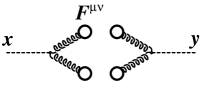
Figure 1: Diagrammatic representation of the contributions to the inclusive $\phi$ spectrum at Leading Order. The dotted line is the free propagator of the scalar particle (eliminated in the spectrum by the action of the operators $\square+m^{2}$). Each spiraling line terminated by a circular blob represents one instance of the gluon field strength at tree level (i.e. it contains terms of order one and two in the gauge field ${\cal A}^{\mu}$).

Thus, at LO, the $\phi$ spectrum is a sum of tree diagrams (see the figure 1). In terms of the classical field strength, the inclusive spectrum for $\phi$ at LO reads simply

$$\left.\frac{dN_{\phi}}{d^{3}{\boldsymbol{p}}}\right|_{{}_{\rm LO}}=\frac{1}{(2\pi)^{3}2E_{\boldsymbol{p}}}\frac{g^{2}_{\phi}}{16}\int d^{4}xd^{4}y\;e^{ip\cdot(x-y)}\;{\cal F}_{\mu\nu}^{a}(x){\cal F}^{\mu\nu,a}(x)\;{\cal F}_{\rho\sigma}^{b}(y){\cal F}^{\rho\sigma,b}(y)\;.$$ (23)

This formula simply expresses the well known fact that, when non-self-interacting particles are produced by an external source, the inclusive spectrum is the modulus squared of the Fourier transform of the source.

3.3 Next-to-Leading Order correction

Let us now consider the production of the $\phi$-particles at NLO, i.e. at the next order in the strong coupling constant $g^{2}$. At the next order, one has two types of contributions:

• 1-loop corrections to the gluon field strength, or to the gluon field strength squared.

• the connected part of $\big{<}\phi_{+}(x)\phi_{-}(y)\big{>}$ at tree level.

These two contributions are illustrated in the figure 2.

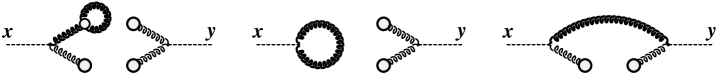
Figure 2: Diagrammatic representation of the contributions to the inclusive $\phi$ spectrum at Next-to-Leading Order. Each blob represents an infinite sum of tree level graphs. The diagram on the left contains the 1-loop correction to $F^{\mu\nu}(x)$. The diagram in the middle involves the connected part of the 1-loop correction to $F^{\mu\nu}(x)F_{\mu\nu}(x)$ (there are two other topologies, not represented here, where the 1-loop correction is on $\Phi_{-}(y)$). The right diagram contains the lowest order connected contribution to $F^{\mu\nu}(x)F^{\rho\sigma}(y)$. Thick lines indicate that the gluon propagators are dressed by the classical background field ${\cal A}^{\mu}$.

These corrections affect only the gluons, and they can be handled in exactly the same way as the corrections to the inclusive gluon spectrum.

The manipulations performed in the previous section for the expectation value of $A^{\mu}(x)A^{\nu}(y)$ can be extended to this more complicated situation, leading the following formal expression for the inclusive $\phi$ spectrum at NLO,

$$\left.\frac{dN_{\phi}}{d^{3}{\boldsymbol{p}}}\right|_{{}_{\rm NLO}}=\Bigg{[}\int\limits_{\Sigma}\!\!d^{3}\vec{\boldsymbol{u}}\,\big{[}\alpha\cdot{\mathbbm{T}}_{\boldsymbol{u}}\big{]}+\frac{1}{2}\sum_{\lambda,a}\!\!\int\frac{d^{3}{\boldsymbol{k}}}{(2\pi)^{3}2k}\!\int\limits_{\Sigma}\!\!d^{3}\vec{\boldsymbol{u}}d^{3}\vec{\boldsymbol{v}}\,\big{[}a_{-{\boldsymbol{k}}\lambda a}\cdot{\mathbbm{T}}_{\boldsymbol{u}}\big{]}\big{[}a_{+{\boldsymbol{k}}\lambda a}\cdot{\mathbbm{T}}_{\boldsymbol{v}}\big{]}\Bigg{]}\,\left.\frac{dN_{\phi}}{d^{3}{\boldsymbol{p}}}\right|_{{}_{\rm LO}}.$$ (24)

In this formula, the inclusive spectrum at leading order should again be considered as a functional of the classical color field ${\cal A}^{\mu}$ on some Cauchy surface $\Sigma$. This relationship is formally identical to the one that relates purely gluonic observables at LO and NLO (e.g. inclusive gluon spectra, or the gluon contribution to the energy-momentum tensor).

In the gluon case, we have shown that it is the integration over ${\boldsymbol{k}}$ in the right hand side of eq. (24) that leads to the logarithms of the CGC cutoffs. Since we have here exactly the same operator, the logarithms that appear in the NLO correction to the inclusive $\phi$ spectrum are identical to those encountered in the gluon spectrum, and they can be resummed into the JIMWLK evolution of the distributions of the sources that produce the color field,

$$\left.\frac{dN_{\phi}}{d^{3}{\boldsymbol{p}}}\right|_{\mbox{\rm Leading Log}}=\int\big{[}D\rho_{1}D\rho_{2}\big{]}\;W_{1}[\rho_{1}]W_{2}[\rho_{2}]\;\left.\frac{dN_{\phi}}{d^{3}{\boldsymbol{p}}}\right|_{{}_{\rm LO}}.$$ (25)

This is another example of the universality of these logarithms.

4 Adjoint scalars

4.1 Model

The simplicity of the previous example is to a large extent due to the fact that the field $\phi$ is not charged under the gauge group of strong interactions. Therefore, the NLO corrections are entirely due to corrections to the gauge fields themselves, and to their two-point correlations.

Things get more complicated when the produced particle carries a color charge. An obvious example is of course that of quarks and antiquarks. However, since quarks also bring the complication of being described by anticommuting fermion fields, let us consider as an intermediate step the case of some hypothetical colored scalar field $\theta_{a}$, that lives in the adjoint representation of the gauge group. The Lagrangian for such scalars is

$${\cal L}\equiv\big{(}D_{\mu}\theta\big{)}_{a}\big{(}D^{\mu}\theta\big{)}^{*}_{a}\;,$$ (26)

where $D_{\mu}$ is the covariant derivative that ensures the minimal coupling of the scalars to the gluons. We assume here that these scalar fields do not interact directly among themselves (i.e. their interactions are always mediated by gluons).

4.2 Inclusive spectrum at LO

The starting point to compute the single inclusive spectrum for the $\theta$ particles is the analogue of eq. (21),

$$\frac{dN_{\theta}}{d^{3}{\boldsymbol{p}}}=\frac{1}{(2\pi)^{3}2p}\sum_{c}\int d^{4}xd^{4}y\;e^{ip\cdot(x-y)}\;\square_{x}\square_{y}\;\big{<}\theta_{+}^{c}(x)\theta_{-}^{c}(y)\big{>}\;,$$ (27)

where $c$ is the color of the produced scalar particle (summed over in the definition of the inclusive spectrum). The two-point correlator under the integral differs from the previous two examples in the fact that it has only connected contributions. This is due to the fact that the Lagrangian (26) is even in the field $\theta$. To stress this property, let us rewrite eq. (27) as follows

$$\frac{dN_{\theta}}{d^{3}{\boldsymbol{p}}}=\frac{1}{(2\pi)^{3}2p}\sum_{c}\int d^{4}xd^{4}y\;e^{ip\cdot(x-y)}\;\square_{x}\square_{y}\;D_{+-}^{cc}(x,y)\;,$$ (28)

where $D_{+-}^{bc}$ is a connected two-point function. The Leading Order contribution to $D_{+-}^{bc}$, that we will denote ${\cal D}_{+-}^{bc}$, is the sum of all the tree level graphs, i.e. the two-point function dressed by the classical color field ${\cal A}^{\mu}$, solution of eq. (3).

Figure 3: Diagrammatic representation of the only contribution to the inclusive $\theta$ spectrum at Leading Order (disconnected graphs cannot exist because the Lagrangian is even in $\theta$). The thick line indicate that the propagator is dressed by insertions of the classical color field ${\cal A}^{\mu}$.

${\cal D}_{+-}^{bc}$ can be expressed in terms of a complete basis of solutions of the scalar wave equation on top of the classical color field ${\cal A}^{\mu}$,

$${\cal D}_{+-}^{bc}(x,y) = \sum_{a}\int\frac{d^{3}{\boldsymbol{q}}}{(2\pi)^{3}2q}\;\vartheta_{-{\boldsymbol{q}}a}^{b}(x)\vartheta_{+{\boldsymbol{q}}a}^{c}(y)$$

$$\left({\cal D}_{\mu}{\cal D}^{\mu}\right)_{cb}\,\vartheta_{\pm{\boldsymbol{q}}a}^{b}(x) = 0\;,\quad\lim_{x^{0}\to-\infty}\vartheta_{\pm{\boldsymbol{q}}a}^{b}(x)=\delta_{ab}e^{\pm iq\cdot x}\;.$$ (29)

In the notation $\vartheta_{\pm{\boldsymbol{q}}a}^{b}$(x), one should not confuse the two color indices $a$ and $b$. The lower index $a$ indicates the color of the wave in the remote past, before it propagates over the classical color field, while the upper index $b$ indicates the color at the point $x$. The fields $\vartheta_{\pm{\boldsymbol{q}}a}$ can be represented diagrammatically as follows :

$$\vartheta_{\pm{\boldsymbol{q}}a}(x)=\raise-22.76219pt\hbox to65.44142pt{\hfil\leavevmode\resizebox{}{56.9055pt}{\includegraphics{theta}}}\;.$$ (30)

In this representation, the red cross represents the initial condition at $x^{0}\to-\infty$, i.e. a plane wave with fixed momentum and color. The arrow is a reminder of the fact that the functions $\vartheta_{\pm{\boldsymbol{q}}a}$ obey retarded boundary conditions set at $x^{0}\to-\infty$. In other words, the propagator that connects the red cross to the point $x$ is a retarded propagator (dressed by the classical color field ${\cal A}^{\mu}$).

In terms of these objects, one can represent the LO propagator ${\cal D}_{+-}$ as

$${\cal D}_{+-}(x,y)=\raise-22.76219pt\hbox to79.6678pt{\hfil\leavevmode\resizebox{}{56.9055pt}{\includegraphics{theta-D}}}\;,$$ (31)

and the $\theta$ spectrum at LO is given by

$$\left.\frac{dN_{\theta}}{d^{3}{\boldsymbol{p}}}\right|_{{}_{\rm LO}}=\frac{1}{(2\pi)^{3}2p}\sum_{a,c}\int\frac{d^{3}{\boldsymbol{q}}}{(2\pi)^{3}2q}\int d^{4}xd^{4}y\;e^{ip\cdot(x-y)}\;\square_{x}\square_{y}\;\vartheta_{-{\boldsymbol{q}}a}^{c}(x)\vartheta_{+{\boldsymbol{q}}a}^{c}(y)\;.$$ (32)

In this formula for the $\theta$ spectrum at leading order, ${\boldsymbol{q}}$ can be interpreted as the momentum of the antiparticle that must necessarily be produced along with the particle of momentum ${\boldsymbol{p}}$ that is tagged in the measurement.

4.3 NLO corrections

4.3.1 List of the 1-loop corrections

$$\underbrace{\raise 2.84526pt\hbox to184.9429pt{\hfil\leavevmode\resizebox{}{48.36958pt}{\includegraphics{scalar-NLO-1}}\hfil}}_{D_{+-}^{(a)}(x,y)}\qquad\underbrace{\raise 2.84526pt\hbox to116.65646pt{\hfil\leavevmode\resizebox{}{48.36958pt}{\includegraphics{scalar-NLO-2}}\hfil}}_{D_{+-}^{(b)}(x,y)}$$

Figure 4: Diagrammatic representation of the contributions to the inclusive $\theta$ spectrum at Next-to-Leading Order. All the lines represent propagators dressed by insertions of the classical color field ${\cal A}^{\mu}$. The blobs indicate that the corresponding vertices are dressed by the background field.

The NLO corrections to the inclusive spectrum of the $\theta$ particles are represented in the figure 4. They can be divided in two distinct categories:

• Tadpole insertions on the propagator of the $\theta$ field, that appear in the first two diagrams of the figure 4. The leftmost correction is the 1-loop correction $\alpha^{\mu}$ to the classical color field ${\cal A}^{\mu}$ that enters in the right hand side of eq. (6). The second diagram is a local self-energy correction on the propagator of the $\theta$ field.

• Non-local 1-loop self-energy correction to the scalar propagator, represented in the third diagram of the figure 4.

4.3.2 Alternate representation

Our goal for the rest of this paper is to write the NLO corrections to the $\theta$ spectrum in a form similar to eqs. (6) and (24). This will be done in several steps. In this subsection, we first rewrite these corrections in a form that resembles eq. (31), in order to highlight the terms that can be seen as mere corrections to one of the functions $\vartheta_{\pm{\boldsymbol{q}}a}$.

This is very simple in the case of the two terms on the left of the figure 4. Indeed, in these two terms the self-energy insertion is a tadpole, that by definition corrects the propagator at a single point. This implies that one can see them as a correction to one of the two factors $\vartheta_{\pm{\boldsymbol{q}}a}$. Let us denote $\zeta_{\pm{\boldsymbol{q}}a}$ this ${\cal O}(g^{2})$ correction to $\vartheta_{\pm{\boldsymbol{q}}a}$,

$$\zeta_{\pm{\boldsymbol{q}}a}^{b}(x)=\raise-25.60747pt\hbox to122.34685pt{\hfil\leavevmode\resizebox{122.34692pt}{}{\includegraphics{zeta}}}\;.$$ (33)

In terms of $\zeta_{\pm{\boldsymbol{q}}a}$, the corresponding NLO corrections to the propagator $D_{+-}$ reads

$$D_{+-}^{(a)}(x,y)=\sum_{a}\int\frac{d^{3}{\boldsymbol{q}}}{(2\pi)^{3}2k}\;\left[\vartheta_{-{\boldsymbol{q}}a}(x)\zeta_{+{\boldsymbol{q}}a}(y)+\zeta_{-{\boldsymbol{q}}a}(x)\vartheta_{+{\boldsymbol{q}}a}(y)\right]\;.$$ (34)

This equation simply states that each of the two factors $\vartheta_{\pm{\boldsymbol{q}}a}$ in eq. (29) has to be corrected in turn. Diagrammatically, this can be represented as

$$D_{+-}^{(a)}(x,y)=\raise-25.60747pt\hbox to150.79959pt{\hfil\leavevmode\resizebox{150.79968pt}{}{\includegraphics{Da}}}\;+[x\leftrightarrow y]\;,$$ (35)

where the unwritten terms, hidden under the abbreviation $[x\leftrightarrow y]$, are the two terms where the tadpole is attached to the leg that ends at the point $y$.

Let us now consider the third diagram on the right of the figure 4. This term is the $+-$ scalar propagator, corrected by a non-local 1-loop self-energy insertion. Because the self-energy is a genuine two-point function, this correction cannot be seen as a correction of either $\vartheta_{+{\boldsymbol{q}}a}$ or $\vartheta_{-{\boldsymbol{q}}a}$ in eq. (29). Instead, we must go back to the Schwinger-Keldysh formalism in order to evaluate this term.

Let us call $\Sigma$ the self-energy. Summing over all the possible assignments of the internal $\pm$ indices in the Schwinger-Keldysh formalism, we can first write

$$D_{+-}^{(b)}={\cal D}_{++}\Sigma_{++}{\cal D}_{+-}-{\cal D}_{++}\Sigma_{+-}{\cal D}_{--}-{\cal D}_{+-}\Sigma_{-+}{\cal D}_{+-}+{\cal D}_{+-}\Sigma_{--}{\cal D}_{--}\;,$$ (36)

where the ${\cal D}_{\pm\pm}$ are the four components of the scalar propagator at tree level. To keep the notations simple, we have not written explicitly the space-time integrations involved in concatenating the self-energy and the tree-level propagators in this equation, but we have of course included the appropriate signs to keep track of the fact that the vertices of type $-$ are opposite to those of type $+$. After some simple algebra, one can rearrange the four terms in the right hand side of the previous equation as follows

$$D_{+-}^{(b)}={\cal D}_{{}_{R}}\Sigma_{{}_{R}}{\cal D}_{+-}+{\cal D}_{{}_{R}}\Sigma_{+-}{\cal D}_{{}_{A}}+{\cal D}_{+-}\Sigma_{{}_{A}}{\cal D}_{{}_{A}}\;,$$ (37)

where the retarded and advanced propagators and self-energies are related to the Schwinger-Keldysh ones by

$${\cal D}_{{}_{R}} \equiv {\cal D}_{++}-{\cal D}_{+-}={\cal D}_{-+}-{\cal D}_{--}$$

$${\cal D}_{{}_{A}} \equiv {\cal D}_{++}-{\cal D}_{-+}={\cal D}_{+-}-{\cal D}_{--}$$

$$\Sigma_{{}_{R}} \equiv \Sigma_{++}-\Sigma_{+-}=\Sigma_{-+}-\Sigma_{--}$$

$$\Sigma_{{}_{A}} \equiv \Sigma_{++}-\Sigma_{-+}=\Sigma_{+-}-\Sigma_{--}\;.$$ (38)

It is interesting to note the pattern in eq. (37) : each term in this formula contains exactly one object of type $+-$. Everything on the left of this object is retarded, and everything on its right is advanced. The three terms of eq. (37) exhaust all the possible locations of the object that carries the $+-$ indices.

For the factors ${\cal D}_{+-}$, we can use eq. (29). In coordinate space, the 1-loop self-energy $\Sigma_{+-}$ is the product of a scalar and a gluon propagator :

$$\Sigma_{+-}\propto{\cal D}_{+-}{\cal G}_{+-}\;,$$ (39)

where the symbol $\propto$ means that we have not written the vertices (they are a bit cumbersome to write because of the possibility of attaching the background field ${\cal A}^{\mu}$ to one leg of the $gg\theta\theta^{*}$ vertex to form an effective $g\theta\theta^{*}$ vertex – how the complete vertices arise will become clear later). In this formula ${\cal G}_{+-}$ is the gluon propagator dressed by insertions of the classical gauge field ${\cal A}^{\mu}$. There is for ${\cal G}_{+-}$ a formula identical to eq. (29),

$${\cal G}_{+-}(x,y)=\sum_{a,\lambda}\int\frac{d^{3}{\boldsymbol{k}}}{(2\pi)^{3}2k}\;a_{-{\boldsymbol{k}}\lambda a}(x)a_{+{\boldsymbol{k}}\lambda a}(y)\;,$$ (40)

where the $a_{\pm{\boldsymbol{k}}\lambda a}$ are now gluonic fluctuations that propagate on top of ${\cal A}^{\mu}$, starting as plane waves of momentum ${\boldsymbol{k}}$, polarization $\lambda$ and color $a$ when $x^{0}\to-\infty$ (see [37] for more details). Mimicking eq. (31), we represent this diagrammatically as follows :

$${\cal G}_{+-}(x,y)=\raise-22.76219pt\hbox to79.6678pt{\hfil\leavevmode\resizebox{}{56.9055pt}{\includegraphics{theta-G}}}\;.$$ (41)

The three terms of eq. (37) can therefore be represented in the following way,

$${\cal D}_{{}_{R}}\Sigma_{{}_{R}}{\cal D}_{+-}=\raise-22.76219pt\hbox to65.44142pt{\hfil\leavevmode\resizebox{}{51.21504pt}{\includegraphics{Db2}}}\quad,\quad{\cal D}_{+-}\Sigma_{{}_{A}}{\cal D}_{{}_{A}}=\raise-22.76219pt\hbox to65.44142pt{\hfil\leavevmode\resizebox{}{51.21504pt}{\includegraphics{Db1}}}$$

$${\cal D}_{{}_{R}}\Sigma_{+-}{\cal D}_{{}_{A}}=\raise-22.76219pt\hbox to65.44142pt{\hfil\leavevmode\resizebox{}{51.21504pt}{\includegraphics{Db3}}}\;,$$ (42)

where the big grey blobs represent the self-energies $\Sigma_{{}_{R,A}}$.

At this point, it is convenient to rewrite the retarded self-energy $\Sigma_{R}$. First of all, one can write

$$\Sigma_{{}_{R}} = \Sigma_{++}-\Sigma_{+-}$$ (43)

$$\propto {\cal G}_{++}{\cal D}_{++}-{\cal G}_{+-}{\cal D}_{+-}$$

$$= {\cal G}_{{}_{R}}{\cal D}_{++}+{\cal G}_{+-}{\cal D}_{{}_{R}}$$

$$= {\cal G}_{{}_{R}}{\cal D}_{-+}+{\cal G}_{+-}{\cal D}_{{}_{R}}\;.$$

In order to obtain the last equality, we must recall that

$${\cal D}_{++}(x,y)=\theta(x^{0}-y^{0})\,{\cal D}_{-+}(x,y)+\theta(y^{0}-x^{0})\,{\cal D}_{+-}(x,y)\;.$$ (44)

Since this propagator is multiplied by the retarded propagator ${\cal G}_{{}_{R}}$, the terms with $\theta(y^{0}-x^{0})$ is forbidden, and we can in fact replace the ${\cal D}_{++}$ by ${\cal D}_{-+}$ to get the final formula. In this rearrangement, we have chosen to break the symmetry between the ${\cal D}$ and ${\cal G}$ propagators in a certain way. It is possible to obtain a more symmetric formula. By doing slightly different transformations, we could alternatively obtain

$$\Sigma_{{}_{R}}\propto{\cal D}_{{}_{R}}{\cal G}_{-+}+{\cal D}_{+-}{\cal G}_{{}_{R}}\;,$$ (45)

and, by combining eqs. (43) and (45),

$$\Sigma_{{}_{R}}\propto\frac{1}{2}{\cal D}_{{}_{R}}({\cal G}_{-+}+{\cal G}_{+-})+\frac{1}{2}({\cal D}_{+-}+{\cal D}_{-+}){\cal G}_{{}_{R}}\;.$$ (46)

Diagrammatically, the expression given in eq. (46) for the retarded self-energy can be represented as follows,

$$\raise-25.60747pt\hbox to122.34692pt{\hfil\leavevmode\resizebox{}{51.21504pt}{\includegraphics{SigR}}}\qquad.$$ (47)

This representation also highlights the different physical meanings of the two terms:

• In the first term, a vacuum fluctuation made of a pair of virtual gluons is created in the past (at the location of the green cross). One of these gluons is absorbed by the scalar fluctuation at the point $u$, and the second of these gluons is absorbed by the same scalar a bit later, at the point $v$.

• In the second term, the vacuum fluctuation created at the location of the red cross is a $\theta\theta^{*}$ fluctuation. One of the scalars from this vacuum fluctuation annihilates the incoming scalar at the point $u$ to form a gluon. Later, at the point $v$, this gluon is absorbed by the second scalar from the vacuum fluctuation to give the outgoing line.

4.4 Expression of the NLO corrections in terms of the operators ${\mathbbm{T}}$

4.4.1 Introduction

Our goal is now to relate the NLO corrections (at the exception of those that involve $\theta\theta^{*}$ vacuum fluctuations – see later) to the LO spectrum by means of a formula similar to eqs. (6) and (24). In order to keep the derivation as intuitive as possible, we will perform this graphically, by using the rules discussed in the section 2.3. Before we proceed, let us summarize the previous discussion by listing all the terms involved in the $\theta$ spectrum at NLO :

$$\raise-28.45274pt\hbox to369.88582pt{\hfil\leavevmode\resizebox{}{113.81102pt}{\includegraphics{NLO-all}}}\qquad.$$ (48)

In these graphs, the red and green crosses are objects that are pinned at $x^{0}=-\infty$ (because they represent the initial condition in the remote past for the scalar waves $\vartheta_{\pm{\boldsymbol{q}}a}$ and gluonic waves $a_{\pm{\boldsymbol{k}}\lambda a}$). The other vertices in these diagrams can be located anywhere in space-time, and the corresponding formulae contain integrals over the positions of all these vertices. In particular, these vertices can be located above or below the Cauchy surface $\Sigma$. The only constraint on their locations is that they are ordered by the causal property of the retarded propagators: the endpoint of a retarded propagator must lie in the future light-cone of its starting point.

4.4.2 Action of the gluonic shifts

As a first step, let us determine the action on the LO spectrum of the operator

$$\int\limits_{\Sigma}\!\!d^{3}\vec{\boldsymbol{u}}\,\big{[}\alpha\cdot{\mathbbm{T}}_{\boldsymbol{u}}\big{]}+\frac{1}{2}\sum_{\lambda,a}\!\!\int\frac{d^{3}{\boldsymbol{k}}}{(2\pi)^{3}2k}\!\int\limits_{\Sigma}\!\!d^{3}\vec{\boldsymbol{u}}d^{3}\vec{\boldsymbol{v}}\,\big{[}a_{-{\boldsymbol{k}}\lambda a}\cdot{\mathbbm{T}}_{\boldsymbol{u}}\big{]}\big{[}a_{+{\boldsymbol{k}}\lambda a}\cdot{\mathbbm{T}}_{\boldsymbol{v}}\big{]}\;,$$ (49)

that appears in eqs. (6) and (24). The ${\mathbbm{T}}$’s contained in this operator act only on the initial condition on $\Sigma$ for the gauge field (implicitly hidden in all the propagators, since they are all dressed by the classical background field). Let us start with the action of $[a\cdot{\mathbbm{T}}_{\boldsymbol{u}}]$ on the LO spectrum. Graphically, we have

$$[a\cdot{\mathbbm{T}}_{\boldsymbol{u}}]\;{\cal D}_{+-}(x,y)=\raise-25.60747pt\hbox to142.26378pt{\hfil\leavevmode\resizebox{}{51.21504pt}{\includegraphics{aT-D}}}\;.$$ (50)

It is equally straightforward to write the action of the quadratic operator $[a\cdot{\mathbbm{T}}_{\boldsymbol{u}}][b\cdot{\mathbbm{T}}_{\boldsymbol{v}}]$ on the leading order expression,

$$[a\cdot{\mathbbm{T}}_{\boldsymbol{u}}][b\cdot{\mathbbm{T}}_{\boldsymbol{v}}]\;{\cal D}_{+-}(x,y)=\raise-82.51299pt\hbox to256.0748pt{\hfil\leavevmode\resizebox{}{179.25244pt}{\includegraphics{abTT-D}}}\;.$$ (51)

When we contract $\alpha(u)$ into ${\mathbbm{T}}_{\boldsymbol{u}}$ and $\frac{1}{2}\sum_{\lambda,a}\int_{\boldsymbol{k}}a_{-{\boldsymbol{k}}\lambda a}(u)a_{+{\boldsymbol{k}}\lambda a}(v)$ into ${\mathbbm{T}}_{\boldsymbol{u}}{\mathbbm{T}}_{\boldsymbol{v}}$, and integrate over $u,v\in\Sigma$, we generate a good deal of the NLO terms in eq. (48). However, by inspection of the graphs that are generated in this operation and by comparing with the list in eq. (48), we readily see that two types of terms are missing:

• The graphs [f,h], where the NLO correction is due to a $\theta\theta^{*}$ vacuum fluctuation, are missing entirely. Having in mind to use this NLO calculation in order to extract the leading logs of energy, we are going to disregard these terms from now on. Indeed, as in the derivation of the BFKL equation, only the gluonic vacuum fluctuations contribute at leading logarithmic accuracy. Scalar or fermionic fluctuations do not contribute to the logarithms at this order, and become necessary only when one goes at the next to leading logarithmic accuracy.

• In the graphs [a,b,c,d,e,g,i], only the portion of the integration domain where the vertices $u$ and $v$ are both above the surface $\Sigma$ are generated. The missing pieces of these graphs are important even at leading log, and in the rest of this section we will show how to generate them.

4.4.3 Scalar shifts

In the terms of eq. (48), when one of the vertices $u$ or $v$ (or both) is located below the surface $\Sigma$, it means that the scalar waves $\vartheta_{\pm{\boldsymbol{q}}a}$ have been affected by the gluonic fluctuation before they reach $\Sigma$. This implies that the corresponding modification to the final observable should be generated by operators that act on the value of the scalar fields on $\Sigma$, instead of the operator ${\mathbbm{T}}_{\boldsymbol{u}}$ that acts on the gluon fields on $\Sigma$.

In order to see this, let us introduce the analogue of the operator ${\mathbbm{T}}_{\boldsymbol{u}}$ for the fields $\vartheta_{\pm{\boldsymbol{q}}a}$. Consider a generic solution of the following equation of motion

$$\left({\cal D}_{\mu}{\cal D}^{\mu}\right)_{cb}\,\vartheta^{b}(x)=0\;,$$ (52)

that describes the propagator of a scalar over some gauge background (The gauge field in the background being fixed.) The Green’s formula for the solutions of this equation reads

$$\vartheta^{b}(x) = i\int\limits_{\Omega}d^{4}y\;D_{{}_{R}}^{0}(x,y)\;\Big{[}2ig{\cal A}_{\mu}(y)\partial^{\mu}_{y}+ig(\partial_{y}^{\mu}{\cal A}_{\mu}(y))+g^{2}{\cal A}_{\mu}(y){\cal A}^{\mu}(y)\Big{]}^{bc}\,\vartheta^{c}(y)$$ (53)

$$\qquad+i\int\limits_{\Sigma}d^{3}\vec{{\boldsymbol{u}}}\;D_{{}_{R}}^{0}(x,u)\;(n\cdot\stackrel{{\scriptstyle\leftrightarrow}}{{\partial}}_{u})\,\vartheta^{b}(u)\;,$$

where $D_{{}_{R}}^{0}$ is the free retarded propagator for the scalar field $\theta$ (i.e. the retarded Green’s function of the D’Alembertian operator $\square_{x}$). The domain $\Omega$ for the integration in the first line is the region of space-time located above the surface $\Sigma$. The term in the second line is a boundary term that contains all the dependence of the solution on its initial condition on $\Sigma$ ($n^{\mu}$ is the normalized vector normal to $\Sigma$ at the point $u$).

Let us now define the following operator,

$$\xi\cdot{\mathbbm{T}}^{\vartheta}_{\boldsymbol{u}}\equiv\xi^{b}(u)\frac{\delta}{\delta\vartheta^{b}(u)}+(n\cdot\partial\xi^{b}(u))\frac{\delta}{\delta(n\cdot\partial\vartheta^{b}(u))}\;,$$ (54)

that mimics for scalar fields the operator ${\mathbbm{T}}_{\boldsymbol{u}}$ that was introduced for gauge fields. Diagrammatically, the action of this operator can be pictured as follows,

$$\big{[}\xi\cdot{\mathbbm{T}}^{\vartheta}_{\boldsymbol{u}}\big{]}\raise-22.76219pt\hbox to48.36958pt{\leavevmode\resizebox{}{56.9055pt}{\hfil\includegraphics{theta1}}}=\;\raise-22.76219pt\hbox to51.21504pt{\leavevmode\resizebox{}{51.21495pt}{\hfill\includegraphics{zeta1}}}\;.$$ (55)

In words, $\xi\cdot{\mathbbm{T}}^{\vartheta}_{\boldsymbol{u}}$ replaces at the point $u\in\Sigma$ the initial value of $\vartheta$ by $\xi(u)$. Thanks to this operator, the perturbation to $\vartheta^{b}(x)$ that results from a perturbation $\xi^{b}(u)$ of its initial condition on the Cauchy surface $\Sigma$ can be written as

$$\xi^{b}(x)=\int\limits_{\Sigma}d^{3}\vec{{\boldsymbol{u}}}\;[\xi\cdot{\mathbbm{T}}^{\vartheta}_{\boldsymbol{u}}]\;\vartheta^{b}(x)\;.$$ (56)

When applying this formalism to the spectrum of the $\theta$ field, we must remember that this spectrum does not depend on a single $\vartheta$ function, but on a an infinite collection of such functions, the $\vartheta_{\pm{\boldsymbol{q}}a}$, for all ${\boldsymbol{q}}$ and $a$. Therefore, we need an operator such as the one defined in eq. (54) for each of them. To avoid the proliferation of notations, we will continue to use the compact notation $\xi\cdot{\mathbbm{T}}^{\vartheta}_{\boldsymbol{u}}$ to denote the sum of these operators for all the relevant fields,

$$\xi\cdot{\mathbbm{T}}^{\vartheta}_{\boldsymbol{u}}\equiv\sum_{a}\sum_{\epsilon=\pm}\int{d^{3}{\boldsymbol{q}}}\;\Bigg{[}\xi^{b}_{\epsilon{\boldsymbol{q}}a}(u)\frac{\delta}{\delta\vartheta^{b}_{\epsilon{\boldsymbol{q}}a}(u)}+(n\cdot\partial\xi^{b}_{\epsilon{\boldsymbol{q}}a}(u))\frac{\delta}{\delta(n\cdot\partial\vartheta^{b}_{\epsilon{\boldsymbol{q}}a}(u))}\Bigg{]}\;.$$ (57)

In order to generate the missing terms in eq. (48) (at the exception of those corresponding to scalar vacuum fluctuations), let us introduce the following two objects

$$\beta(u) \equiv \raise-22.76219pt\hbox to153.6447pt{\hfil\leavevmode\resizebox{}{56.9055pt}{\includegraphics{beta}}\hfil}\;,$$

$$\zeta_{{\boldsymbol{k}}\lambda a}(u) \equiv \raise-25.60747pt\hbox to51.21504pt{\hfil\leavevmode\resizebox{}{56.9055pt}{\includegraphics{zeta_k}}\hfil}\;.$$ (58)

It is now possible to generate the missing terms as follows :

• The operator $\beta\cdot{\mathbbm{T}}^{\vartheta}$ will generate the terms of eq. (48) where the two vertices $u$ and $v$ are attached to the same scalar line and are both below the surface $\Sigma$.

• The operator $\frac{1}{2}[\zeta_{-{\boldsymbol{k}}\lambda a}\cdot{\mathbbm{T}}^{\vartheta}][\zeta_{+{\boldsymbol{k}}\lambda a}\cdot{\mathbbm{T}}^{\vartheta}]$ generates the part of the term [i] of eq. (48), where the vertices $u$ and $v$ are both below $\Sigma$.

• In order to produce the part of the terms [e,g,i] where one of the vertices $u$ and $v$ is above $\Sigma$ while the other is below, we must act with the operator

  $$\frac{1}{2}[a_{-{\boldsymbol{k}}\lambda a}\cdot{\mathbbm{T}}][\zeta_{+{\boldsymbol{k}}\lambda a}\cdot{\mathbbm{T}}^{\vartheta}]+\frac{1}{2}[\zeta_{-{\boldsymbol{k}}\lambda a}\cdot{\mathbbm{T}}^{\vartheta}][a_{+{\boldsymbol{k}}\lambda a}\cdot{\mathbbm{T}}]\;,$$ (59)

  that mixes the gluonic and the scalar shifts.

4.4.4 Final form of the NLO spectrum

Let us now summarize this section by collecting all the terms together. At the exception of the contribution of the scalar vacuum fluctuations, the NLO correction to the $\theta$ inclusive spectrum can be written as follows,

$$\left.\frac{dN_{\theta}}{d^{3}{\boldsymbol{p}}}\right|_{{}_{\rm NLO}}=\Bigg{[}\int\limits_{\Sigma}d^{3}\vec{\boldsymbol{u}}\,\big{[}\alpha\cdot{\mathbbm{T}}_{\boldsymbol{u}}+\beta\cdot{\mathbbm{T}}_{\boldsymbol{u}}^{\vartheta}\big{]}+$$

$$+\frac{1}{2}\sum_{\lambda,a}\int\frac{d^{3}{\boldsymbol{k}}}{(2\pi)^{3}2k}\int\limits_{\Sigma}d^{3}\vec{\boldsymbol{u}}d^{3}\vec{\boldsymbol{v}}\,\big{[}a_{-{\boldsymbol{k}}\lambda a}\cdot{\mathbbm{T}}_{\boldsymbol{u}}+\zeta_{-{\boldsymbol{k}}\lambda a}\cdot{\mathbbm{T}}_{\boldsymbol{u}}^{\vartheta}\big{]}\big{[}a_{+{\boldsymbol{k}}\lambda a}\cdot{\mathbbm{T}}_{\boldsymbol{v}}+\zeta_{+{\boldsymbol{k}}\lambda a}\cdot{\mathbbm{T}}_{\boldsymbol{u}}^{\vartheta}\big{]}\Bigg{]}\,\left.\frac{dN_{\theta}}{d^{3}{\boldsymbol{p}}}\right|_{{}_{\rm LO}}\;.$$

(60)

This formula is the main result of this paper. It generalizes the eqs. (6) and (24) to the case of a theory involving new colored fields in addition to the gluons. The general structure of the operator that relates the NLO correction to the LO is preserved by this new formula, and the generalization simply amounts to introducing new terms that involve derivatives with respect to the initial value of the scalar fields.

Although we have derived it here for scalar fields, a structurally identical formula can be derived for quark production. The NLO topologies in eq. (48) are the same for the quark spectrum, at the exception of $[{\bf b,d}]$ that do not exist for quarks due to the absence of $q\bar{q}gg$ coupling. We have sketched the derivation of the quark analogue of eq. (60) in the appendix A.

4.5 Discussion on factorization

In the case of the gluon spectra, the identity (6) was essential in order to extract the logarithms of the CGC cutoff $\Lambda$, and to prove that these logarithms can be factorized into distributions of color sources that evolve according to the JIMWLK equation. The reason for this is that, if one chooses the Cauchy surface $\Sigma$ to be just above the past light-cone, then all these logarithms are contained in the operator that relates LO and NLO, as stated by the equation (7). From this formula, factorization follows easily thanks to the Hermiticity of the JIMWLK Hamiltonian (see [37] for details).

Obviously, the operator in the left hand side of eq. (7) is contained in the operator that appears in the right hand side of eq. (60), and as a consequence we already know that the NLO $\theta$ spectrum contains logarithms proportional to the JIMWLK Hamiltonian. However, it is crucial to note that we do not get the complete Hamiltonian here: we get the JIMWLK Hamiltonian restricted to act only on the color sources contained in the gluon fields on $\Sigma$. This is because it is derived from the operators ${\mathbbm{T}}$, that act only on the initial gauge fields, but not on the scalar fields. In other words, it would be more correct to write

$$\int\limits_{\Sigma}\!\!d^{3}\vec{\boldsymbol{u}}\,\big{[}\alpha\cdot{\mathbbm{T}}_{\boldsymbol{u}}\big{]}+\frac{1}{2}\sum_{\lambda,a}\!\!\int\frac{d^{3}{\boldsymbol{k}}}{(2\pi)^{3}2k}\!\int\limits_{\Sigma}\!\!d^{3}\vec{\boldsymbol{u}}d^{3}\vec{\boldsymbol{v}}\,\big{[}a_{-{\boldsymbol{k}}\lambda a}\cdot{\mathbbm{T}}_{\boldsymbol{u}}\big{]}\big{[}a_{+{\boldsymbol{k}}\lambda a}\cdot{\mathbbm{T}}_{\boldsymbol{v}}\big{]}=$$

$$\qquad\qquad\qquad\qquad\qquad=\log(\Lambda^{+})\,{\cal H}_{1}^{{}_{A}}+\log(\Lambda^{-})\,{\cal H}_{2}^{{}_{A}}+\mbox{terms w/o logs}\;,$$ (61)

where ${\cal H}_{1,2}^{{}_{A}}$ is this restricted JIMWLK Hamiltonian that acts only on gluons.

For factorization to be valid for scalar production, we would also need the missing parts of the Hamiltonian, that act on the initial scalar fields. This is presumably the role of the additional terms in the operator that appears in eq. (60). Indeed, these terms involve the new shift operator ${\mathbbm{T}}^{\vartheta}$, that precisely acts on the initial value of the scalar fields. We are thus led to conjecture an extension of eq. (7), that reads

$$\int\limits_{\Sigma}d^{3}\vec{\boldsymbol{u}}\,\big{[}\alpha\cdot{\mathbbm{T}}_{\boldsymbol{u}}+\beta\cdot{\mathbbm{T}}_{\boldsymbol{u}}^{\vartheta}\big{]}+$$

$$\qquad+\frac{1}{2}\sum_{\lambda,a}\int\frac{d^{3}{\boldsymbol{k}}}{(2\pi)^{3}2k}\int\limits_{\Sigma}d^{3}\vec{\boldsymbol{u}}d^{3}\vec{\boldsymbol{v}}\,\big{[}a_{-{\boldsymbol{k}}\lambda a}\cdot{\mathbbm{T}}_{\boldsymbol{u}}+\zeta_{-{\boldsymbol{k}}\lambda a}\cdot{\mathbbm{T}}_{\boldsymbol{u}}^{\vartheta}\big{]}\big{[}a_{+{\boldsymbol{k}}\lambda a}\cdot{\mathbbm{T}}_{\boldsymbol{v}}+\zeta_{+{\boldsymbol{k}}\lambda a}\cdot{\mathbbm{T}}_{\boldsymbol{u}}^{\vartheta}\big{]}=$$

$$\qquad=\log(\Lambda^{+})\,{\cal H}_{1}+\log(\Lambda^{-})\,{\cal H}_{2}+\mbox{terms w/o logs}\;,$$ (62)

where now ${\cal H}_{1,2}$ is the full JIMWLK Hamiltonian that acts both on the color sources contained in gauge fields and in scalar fields. This formula, if true, would immediately imply the factorizability of the leading logarithms of the $\theta$ spectrum into the universal distributions $W$. However, proving eq. (62) requires extracting the logarithms coming from the new terms of eq. (60) and showing that their coefficients recombine nicely to form the kernel of the JIMWLK Hamiltonian. We stress that this has not been done at the moment.

5 Summary and outlook

In this paper, we have derived generalizations of an identity that plays a crucial role in the proof of factorization of high energy logarithms in heavy ion collisions. This functional relationship, that relates the leading order and next-to-leading order contributions to inclusive observables, is a central step in factorization because it highlights the causal aspects of a collision process, by separating what happens before the collision from what happens after.

The generalization we have obtained goes in the direction of extending the field content of the theory under consideration. To the gluons already present in all the known examples of this factorization, we have added scalar fields that couple in some way to the gluons. The simplest extension is that of color neutral scalar particles. Because they are not colored, the formula that was already known for gluons is valid without change in this situation.

Then, we have considered a much more complicated example, involving colored scalar particles, that interact non trivially with the gauge fields. In this case, the formula that was valid for the pure glue case must be slightly modified. We have shown that this can be done by a very natural extension of the formalism: we also need operators that differentiate with respect to the initial value of the scalar fields. Thanks to this generalization, it is also possible to obtain a functional relationship between the LO and NLO contributions.

An obvious extension of this work is to use eq. (60) in order to extract the logarithms of the CGC cutoffs, and to prove that they can be absorbed into the JIMWLK evolved $W$ distributions that already appear in purely gluonic observables, providing further evidence of their universality. Naturally, this would be most interesting in the case of the quark inclusive spectrum, for which we have outlined the relevant NLO formula in the appendix A.

A more remote application of the same ideas and tools is to study the logarithms that arise in gluon production beyond leading logarithmic accuracy, in order to obtain the first $\alpha_{s}$ correction to the JIMWLK Hamiltonian. The first step in this program is to derive the inclusive gluon spectrum at NNLO, i.e. at two loops. Some of the topologies one would need to evaluate in this calculation are very similar to the graphs we have studied in the section 4. If one wants to extend the factorization proof of [37] beyond leading logarithmic accuracy, an important intermediate step would be to find a functional relationship between the gluon spectra at NNLO and LO, similar to eq. (6).

There is another, much more intriguing and difficult, direction in which one could try to extend these factorization results – that of exclusive observables, e.g. the cross section for events with a rapidity gap. In the case of exclusive observables, the strategy for establishing factorization that we have employed in [37] fails at the first stage: so far we have not been able to obtain formulae such as eqs. (6), (24) and (60) for any exclusive observable. The main obstacle in obtaining similar formulae in this case seems to be that these exclusive observables are expressible in terms of classical fields with non-retarded boundary conditions [45] (for instance boundary conditions that constrain the fields both at $x^{0}=-\infty$ and at $x^{0}=+\infty$).

Appendix A Inclusive quark spectrum

The calculation of the inclusive spectrum at LO and NLO for charged scalar fields, that we have presented in the section 4, can easily be generalized to the case of quark production. Now the Lagrangian density that couples the quarks and antiquarks to the gluons is

$${\cal L}\equiv i\overline{\psi}\,\raise 0.6458pt\hbox{$/$}\kern-7.29996pt\hbox{$D$}\,\psi\;,$$ (63)

where $\psi$ is the spinor for one quark flavor (we disregard the quark mass, that does not play any role in this discussion). This Lagrangian is quadratic in the fermion fields, which means that the quarks do not interact directly among themselves. In terms of its interactions, this theory is in fact a bit simpler than the theory of charged scalars, since it has only a $q\overline{q}g$ vertex and no derivative couplings.

The inclusive quark spectrum is given to all orders by a formula which is very similar to eq. (28),

$$\frac{dN_{\rm q}}{d^{3}{\boldsymbol{p}}}=\frac{1}{(2\pi)^{3}2p}\sum_{s,i}\int d^{4}xd^{4}y\;e^{ip\cdot(x-y)}\;(u_{s}({\boldsymbol{p}})\raise 0.6458pt\hbox{$/$}\kern-5.29999pt\hbox{$\partial$}_{x})(u^{\dagger}_{s}({\boldsymbol{p}})\raise 0.6458pt\hbox{$/$}\kern-5.29999pt\hbox{$\partial$}_{y})\;S_{+-}^{ii}(x,y)\;,$$ (64)

where $u_{s}({\boldsymbol{p}})$ is a free spinor representing a quark of momentum ${\boldsymbol{p}}$ and spin $s$, and $S_{+-}^{ij}(x,y)$ is the $+-$ component of the quark two-point function in the Schwinger-Keldysh formalism (we use latin letters $i,j,k$ for colors indices in the fundamental representation). Note that the inclusive spectrum is summed over all spin states $s$ and colors $i$ of the produced quark.

At leading order, we can represent this two-point function in terms of a complete basis of solutions of the Dirac equation in the background field ${\cal A}^{\mu}$,

$${\cal S}_{+-}^{ij}(x,y) = \sum_{s,k}\int\frac{d^{3}{\boldsymbol{q}}}{(2\pi)^{3}2q}\;\psi^{\dagger i}_{{\boldsymbol{q}}sk}(x)\psi^{j}_{{\boldsymbol{q}}sk}(y)$$

$$i\raise 0.6458pt\hbox{$/$}\kern-6.30005pt\hbox{$\cal D$}_{ij}\,\psi^{j}_{{\boldsymbol{q}}sk}(x) = 0\;,\quad\lim_{x^{0}\to-\infty}\psi^{i}_{{\boldsymbol{q}}sk}(x)=\delta_{ik}\,v_{s}({\boldsymbol{q}})\,e^{iq\cdot x}\;.$$ (65)

Here also, the lower color index is the color of the quark at $x^{0}=-\infty$, while $i$ is its color at the current time $x^{0}$. Eqs. (64) and the representation (65) were the basis of the numerical evaluation of the quark spectrum in the CGC framework done in [28, 29].

At NLO, we need to evaluate the 1-loop corrections to the two-point function $S_{+-}$. The relevant topologies are those listed in the figure 5.

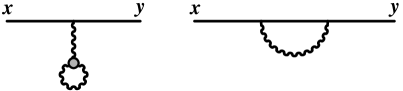
Figure 5: Diagrammatic representation of the contributions to the inclusive quark spectrum at Next-to-Leading Order. All the lines represent propagators dressed by insertions of the classical color field ${\cal A}^{\mu}$. The blobs indicate that the corresponding vertices are dressed by the background field.

One of the topologies present in the scalar case does not exist for quarks, since there is no $q\overline{q}gg$ elementary vertex. For the same reason, the $q\overline{q}g$ vertex cannot be dressed by the background field. After some transformations identical to those performed in the section 4.3.2, we can represent the NLO contributions to the quark spectrum in the following form, which is more appropriate for our purposes:

$$\raise-28.45274pt\hbox to369.88582pt{\hfil\leavevmode\resizebox{}{113.81102pt}{\includegraphics{q-NLO-all}}}\quad.$$ (66)

Compared to eq. (48), two graphs have disappeared, and all the $q\overline{q}g$ vertices are bare vertices. Like in the scalar case, all the NLO terms that involve gluonic vacuum fluctuations (i.e. all the above terms except the graphs [f,h]) can be related to the LO spectrum as follows,

$$\left.\frac{dN_{\rm q}}{d^{3}{\boldsymbol{p}}}\right|_{{}_{\rm NLO}}=\Bigg{[}\int\limits_{\Sigma}d^{3}\vec{\boldsymbol{u}}\,\big{[}\alpha\cdot{\mathbbm{T}}_{\boldsymbol{u}}+\beta\cdot{\mathbbm{T}}_{\boldsymbol{u}}^{\rm Q}\big{]}+$$

$$+\frac{1}{2}\sum_{\lambda,a}\int\frac{d^{3}{\boldsymbol{k}}}{(2\pi)^{3}2k}\int\limits_{\Sigma}d^{3}\vec{\boldsymbol{u}}d^{3}\vec{\boldsymbol{v}}\,\big{[}a_{-{\boldsymbol{k}}\lambda a}\cdot{\mathbbm{T}}_{\boldsymbol{u}}+\zeta_{-{\boldsymbol{k}}\lambda a}\cdot{\mathbbm{T}}_{\boldsymbol{u}}^{\rm Q}\big{]}\big{[}a_{+{\boldsymbol{k}}\lambda a}\cdot{\mathbbm{T}}_{\boldsymbol{v}}+\zeta_{+{\boldsymbol{k}}\lambda a}\cdot{\mathbbm{T}}_{\boldsymbol{u}}^{\rm Q}\big{]}\Bigg{]}\,\left.\frac{dN_{\rm q}}{d^{3}{\boldsymbol{p}}}\right|_{{}_{\rm LO}}\;.$$

(67)

All the differences between adjoint scalars and quarks are now hidden in the definitions of the objects $\beta$ and $\zeta_{\pm{\boldsymbol{k}}\lambda a}$, that are now given by

$$\beta(u)\equiv\raise-22.76219pt\hbox to113.81102pt{\hfil\leavevmode\resizebox{}{56.9055pt}{\includegraphics{q-beta}}\hfil}\;,\quad\zeta_{{\boldsymbol{k}}\lambda a}(u)\equiv\raise-25.60747pt\hbox to51.21504pt{\hfil\leavevmode\resizebox{}{56.9055pt}{\includegraphics{q-zeta_k}}\hfil}\;,$$ (68)

and in the definition of the operator ${\mathbbm{T}}_{\boldsymbol{u}}^{\rm Q}$ that replaces ${\mathbbm{T}}_{\boldsymbol{u}}^{\vartheta}$. This new operator generates shifts of the initial condition of a spinor on the Cauchy surface $\Sigma$, and eq. (54) is replaced by

$$\xi\cdot{\mathbbm{T}}^{\rm Q}_{\boldsymbol{u}}\equiv(\raise 0.6458pt\hbox{$/$}\kern-5.29999pt\hbox{$n$}\xi^{i}(u))\frac{\delta}{\delta(\raise 0.6458pt\hbox{$/$}\kern-5.29999pt\hbox{$n$}\psi^{i}(u))}\;.$$ (69)

References

- [1] F.D. Aaron, et al, [H1 and ZEUS Collaborations] JHEP 1001, 109 (2010).
- [2] I. Balitsky, L.N. Lipatov, Sov. J. Nucl. Phys. 28, 822 (1978).
- [3] E.A. Kuraev, L.N. Lipatov, V.S. Fadin, Sov. Phys. JETP 45, 199 (1977).
- [4] Yu.V. Kovchegov, K. Tuchin, Phys. Rev. D 65, 074026 (2002).
- [5] A. Dumitru, L.D. McLerran, Nucl. Phys. A 700, 492 (2002).
- [6] J.P. Blaizot, F. Gelis, R. Venugopalan, Nucl. Phys. A 743, 13 (2004).
- [7] G.A. Chirilli, B.-W. Xiao, F. Yuan, Phys. Rev. D 86, 054005 (2012).
- [8] E. Avsar, arXiv:1108.1181.
- [9] E. Avsar, arXiv:1203.1916.
- [10] J.F. Gunion, G. Bertsch, Phys. Rev. D 25, 746 (1982).
- [11] J.C. Collins, R.K. Ellis, Nucl. Phys. B 360, 3 (1991).
- [12] S. Catani, M. Ciafaloni, F. Hautmann, Nucl. Phys. B 366, 135 (1991).
- [13] L.V. Gribov, E.M. Levin, M.G. Ryskin, Phys. Rept. 100, 1 (1983).
- [14] J. Jalilian-Marian, A. Kovner, L.D. McLerran, H. Weigert, Phys. Rev. D 55, 5414 (1997).
- [15] J. Jalilian-Marian, A. Kovner, A. Leonidov, H. Weigert, Nucl. Phys. B 504, 415 (1997).
- [16] J. Jalilian-Marian, A. Kovner, A. Leonidov, H. Weigert, Phys. Rev. D 59, 014014 (1998).
- [17] J. Jalilian-Marian, A. Kovner, A. Leonidov, H. Weigert, Phys. Rev. D 59, 034007 (1999).
- [18] J. Jalilian-Marian, A. Kovner, A. Leonidov, H. Weigert, Phys. Rev. D 59, 099903 (1999).
- [19] E. Iancu, A. Leonidov, L.D. McLerran, Nucl. Phys. A 692, 583 (2001).
- [20] E. Iancu, A. Leonidov, L.D. McLerran, Phys. Lett. B 510, 133 (2001).
- [21] E. Iancu, A. Leonidov, L.D. McLerran, Lectures given at Cargese Summer School on QCD Perspectives on Hot and Dense Matter, Cargese, France, 6-18 Aug 2001, hep-ph/0202270.
- [22] E. Iancu, R. Venugopalan, Quark Gluon Plasma 3, Eds. R.C. Hwa and X.N. Wang, World Scientific, hep-ph/0303204.
- [23] F. Gelis, E. Iancu, J. Jalilian-Marian, R. Venugopalan, Ann. Rev. Part. Nucl. Sci. 60, 463 (2010).
- [24] L.D. McLerran, R. Venugopalan, Phys. Rev. D 49, 2233 (1994).
- [25] L.D. McLerran, R. Venugopalan, Phys. Rev. D 49, 3352 (1994).
- [26] L.D. McLerran, R. Venugopalan, Phys. Rev. D 50, 2225 (1994).
- [27] F. Gelis, R. Venugopalan, Nucl. Phys. A 776, 135 (2006).
- [28] F. Gelis, K. Kajantie, T. Lappi, Phys. Rev. C. 71, 024904 (2005).
- [29] F. Gelis, K. Kajantie, T. Lappi, Phys. Rev. Lett. 96, 032304 (2006).
- [30] A. Krasnitz, R. Venugopalan, Phys. Rev. Lett. 84, 4309 (2000).
- [31] A. Krasnitz, R. Venugopalan, Phys. Rev. Lett. 86, 1717 (2001).
- [32] A. Krasnitz, R. Venugopalan, Nucl. Phys. B 557, 237 (1999).
- [33] A. Krasnitz, Y. Nara, R. Venugopalan, Nucl. Phys. A 727, 427 (2003).
- [34] A. Krasnitz, Y. Nara, R. Venugopalan, Phys. Rev. Lett. 87, 192302 (2001).
- [35] A. Krasnitz, Y. Nara, R. Venugopalan, Nucl. Phys. A 717, 268 (2003).
- [36] T. Lappi, Phys. Rev. C 67, 054903 (2003).
- [37] F. Gelis, T. Lappi, R. Venugopalan, Phys. Rev. D 78, 054019 (2008).
- [38] F. Gelis, T. Lappi, R. Venugopalan, Phys. Rev. D 78, 054020 (2008).
- [39] F. Gelis, T. Lappi, R. Venugopalan, Phys. Rev. D 79, 094017 (2009).
- [40] T. Liou, arXiv:1206.6123.
- [41] I. Balitsky, Phys. Rev. D 75, 014001 (2007).
- [42] I. Balitsky, G.A. Chirilli, Phys. Rev. D 77, 014019 (2008).
- [43] Yu.V. Kovchegov, H. Weigert, Nucl. Phys. A 784, 188 (2007).
- [44] E. Gardi, J. Kuokkanen, K. Rummukainen, H. Weigert, Nucl. Phys. A 784, 282 (2007).
- [45] F. Gelis, R. Venugopalan, Nucl. Phys. A 779, 177 (2006).