DBKGrad: An R Package for Mortality Rates Graduation by Fixed and Adaptive
Discrete Beta Kernel Techniques

Angelo Mazza, Antonio Punzo dbkGrad: An R Package for Graduation by Discrete Beta Kernel Techniques DBKGrad: An R Package for Graduation by Discrete Beta Kernel Techniques Kernel smoothing represents a useful approach in the graduation of mortality rates. Though there exist several options for performing kernel smoothing in statistical software packages, there have been very few contributions to date that have focused on applications of these techniques in the graduation context. Also, although it has been shown that the use of a variable or adaptive smoothing parameter, based on the further information provided by the exposed to the risk of death, provides additional benefits, specific computational tools for this approach are essentially absent. Furthermore, little attention has been given to providing methods in available software for any kind of subsequent analysis with respect to the graduated mortality rates. To facilitate analyses in the field, the R package DBKGrad is introduced. Among the available kernel approaches, it considers a recent discrete beta kernel estimator, in both its fixed and adaptive variants. In this approach, boundary bias is automatically reduced and age is pragmatically considered as a discrete variable. The bandwidth, fixed or adaptive, is allowed to be manually given by the user or selected by cross-validation. Pointwise confidence intervals, for each considered age, are also provided. An application to mortality rates from the Sicily Region (Italy) for the year 2008 is also presented to exemplify the use of the package. kernel smoothing, graduation, beta distribution, cross-validation Antonio Punzo
Dipartimento di Economia e Impresa
Università di Catania
95129 Catania, Italia
Telephone: +39/095/7537640
Fax: +39/095/7537610
E-mail:
URL: http://www.economia.unict.it/punzo

1 Introduction

Mortality rates are age-specific indicators commonly used in demography. Historically, they are also widely adopted by actuaries, in the form of mortality tables, to calculate life insurance premiums, annuities, reserves, and so on. Producing these tables from a suitable set of crude (or raw) mortality rates is called graduation, and this subject has been extensively discussed in the actuarial literature (see, e.g., Copas and Haberman 1983 and Haberman and Renshaw 1996). To be specific, the $d_{x}$ deaths at age $x$ can be seen as arising from a population, initially exposed to the risk of death, of size $e_{x}$. The situation is commonly summarized via the model $d_{x}\sim\text{Bin}\left(e_{x},q_{x}\right)$, where $q_{x}$ represents the true, but unknown, mortality rate at age $x$. The crude rate $\mathring{q}_{x}$ is the observed counterpart of $q_{x}$. Graduation is necessary because crude data usually presents abrupt changes, which do not agree to the dependence structure supposedly characterizing the true rates (London, 1985). In fact, a common prior opinion about their form is that each true mortality rate is closely related to its neighbors. This relationship is expressed by the belief that the true rates progress smoothly from one age to the next. So, the next logical step is to graduate the crude rates to produce smooth estimates, $\widehat{q}_{x}$, of the true rates. This is done by systematically revising the crude rates in order to remove any random fluctuations. Nonparametric models are the natural choice if the aim is to reflect this belief. Furthermore, a nonparametric approach can be used to choose the simplest suitable parametric model, to provide a diagnostic check of a parametric model, or to simply explore the data (see Härdle 1992, Section 1.1, for a detailed discussion on the chief motivations that imply their use, and Debòn et al. 2006 for an exhaustive comparison of nonparametric methods in the graduation of mortality rates).

Due to its conceptual simplicity and practical and theoretical properties, kernel smoothing is one of the most popular statistical methods for nonparametric graduation. Among the various alternatives existing in literature (see Copas and Haberman 1983, Gavin et al. 1993, 1994, 1995 and Peristera and Kostaki 2005), the attention is here focused on the discrete beta kernel estimator proposed by Mazza and Punzo (2011). Roughly speaking, the genesis of this model starts with the consideration that, although age $X$ is in principle a continuous variable, it is typically truncated in some way, such as age at last birthday, so that it takes values on the discrete set $\mathcal{X}=\left\{0,1,\ldots,\omega\right\}$, $\omega$ being the highest age of interest. Discretization of age, from a pragmatical and practical point of view, could also come handy to actuaries that have to produce “discrete” graduated mortality tables starting from the observed counterparts. In the fixed bandwidth estimator proposed in Mazza and Punzo (2011), the discrete beta probability mass functions of Punzo and Zini (2012), parameterized according to Punzo (2010, see also , ), are considered as kernel functions in order to overcome the problem of boundary bias, commonly arising from the use of symmetric kernels (see Chen, 2000). The support $\mathcal{X}$ of the discrete beta, in fact, matches the age range and this, when smoothing is made near the boundaries, allows avoiding allocation of weight outside the support (for example negative or unrealistically high ages). Variants of the fixed bandwidth discrete beta kernel estimator, which allow the bandwidth to vary at each age according to the reliability of the data, also exist; in Mazza and Punzo (2013), the reliability is expressed by the $e_{x}$, while in Mazza and Punzo (in press) this reliability is measured via the reciprocal of the variation coefficient (VC), with the VC being function of both the amount of exposure and the observed mortality rate.

In this paper we present the R (R Development Core Team, 2012) package DBKGrad, available from CRAN (http://CRAN.R-project.org/), which offers all the features described above and adds some related functionalities. Although R is well-provided with kernel smoothing techniques (see, e.g., Hayfield and Racine, 2008), it does not offer neither discrete beta kernel smoothing, nor application of kernel smoothing techniques in graduation of mortality data. Note that nonparametric smoothing techniques, of the kind found in DBKGrad, are commonly used and often cited exploratory statistical tools; as evidence, consider the number of times in which classical statistical studies use the functions density and ksmooth, both in the stats package, for kernel smoothing estimation of a density or regression function.

The paper is organized as follows. Section 2 retraces the fixed discrete beta kernel estimator. Its adaptive variants are recalled in Section 3 while some cross-validation approaches for the selection of both the fixed and the adaptive bandwidth is discussed in Section 4. Further related aspects, such as the adoption of a preliminary logit transformation of the rates and the computation of the pointwise confidence intervals, are given in Section 5. The relevance of the DBKGrad package is shown, via a real data set, in Section 6, and conclusions are finally given in Section 7.

2 Discrete beta kernel graduation

Given the crude rates $\mathring{q}_{y}$, $y\in\mathcal{X}$, the Nadaraya-Watson kernel estimator of the true but unknown mortality rate $q_{x}$, at the evaluation age $x$, is

$$\widehat{q}_{x}=\sum_{y\in\mathcal{X}}\frac{k_{h}\left(y;m=x\right)}{\displaystyle\sum_{j\in\mathcal{X}}k_{h}\left(j;m=x\right)}\mathring{q}_{y}=\sum_{y\in\mathcal{X}}K_{h}\left(y;m=x\right)\mathring{q}_{y},\quad x\in\mathcal{X},$$ (1)

where $k_{h}\left(\cdot;m\right)$ is the discrete kernel function (hereafter simply named kernel), $m\in\mathcal{X}$ is the single mode of the kernel, $h>0$ is the (fixed) bandwidth (or smoothing parameter) governing the bias-variance trade-off, and $K_{h}\left(\cdot;m\right)$ is the normalized kernel. Since we are treating age as being discrete, with equally spaced values, kernel graduation by means of (1) is equivalent to moving (or local) weighted average graduation (Gavin et al., 1995).

In (1), the discrete beta kernels (Mazza and Punzo, 2011)

$$k_{h}\left(x;m\right)=\displaystyle\left(x+\frac{1}{2}\right)^{\frac{m+\frac{1}{2}}{h\left(\omega+1\right)}}\displaystyle\left(\omega+\frac{1}{2}-x\right)^{\frac{\omega+\frac{1}{2}-m}{h\left(\omega+1\right)}}$$ (2)

are here adopted. Their normalized version,

$$K_{h}\left(x;m\right)=\frac{k_{h}\left(x;m\right)}{\displaystyle\sum_{y\in\mathcal{X}}k_{h}\left(y;m\right)},$$

corresponds to the discrete beta probability mass function defined in Punzo and Zini (2012) and parameterized, as in Punzo (2010), according to the mode $m$ and another parameter $h$ that is closely related to the distribution variability. In particular, for $h\rightarrow 0^{+}$, $K_{h}\left(x;m\right)$ tends to a Dirac delta function in $x=m$, while for $h\rightarrow\infty$, $K_{h}\left(x;m\right)$ tends to a discrete uniform distribution; Figure 1 shows the effect of varying $h$, maintaining constant $\omega$ and $m$.

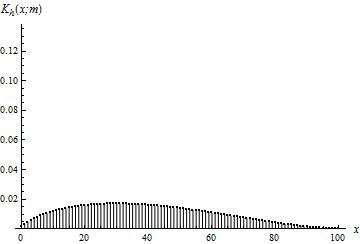
(a) $h=0.4$

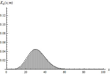
(b) $h=0.04$

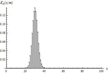
(c) $h=0.004$

Figure 1: The effect of varying $h$ in the discrete beta probability mass function ($\omega=100$ and $m=30$).

Thus $h$ can be considered as the smoothing parameter of the estimator (1); indeed, as $h$ becomes smaller, the spurious fine structure becomes visible, while as $h$ gets larger, more details are obscured.

Roughly speaking, discrete beta kernels possess two peculiar characteristics. Firstly, their shape, fixed $h$, automatically changes according to the value of $m$. The graphical effect of varying $m$, keep fixed $h$ and $\omega$, is displayed in Figure 2.

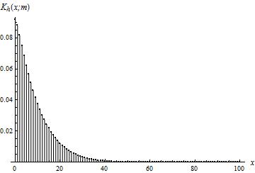
(a) $m=0$

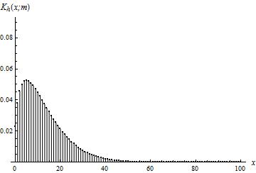
(b) $m=5$

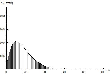
(c) $m=10$

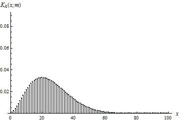
(d) $m=20$

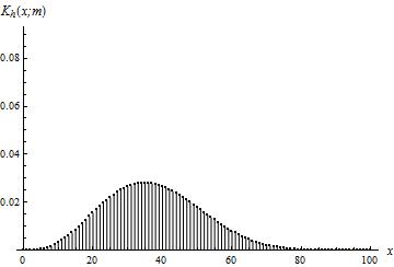
(e) $m=35$

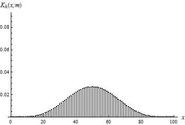
(f) $m=50$

Figure 2: The effect of varying $m$ in the discrete beta probability mass function ($\omega=100$ and $h=0.1$).

Secondly, the support of the kernels matches the age range $\mathcal{X}$ so that no weight is assigned outside the data support; this means that the order of magnitude of the bias does not increase near the boundaries. Further details are reported in Mazza and Punzo (2011); see also Chen (2000) to find out more on the properties of the discrete beta kernel estimator in its continuous counterpart. The discrete beta kernel estimator is obtained with the specification bandwidth="FX" – which represents the default – in the dbkGrad function.

3 Making the bandwidth adaptive

Rather than restricting $h$ to a fixed value, a more flexible approach is to allow the bandwidth to vary according to the reliability of the data measured in a convenient way. Thus, for ages in which the reliability is relatively larger, a low value for $h$ results in an estimate that more closely reflects the crude rates. For ages in which the reliability is smaller, such as at old ages, a higher value for $h$ allows the estimate of the true mortality rates to progress more smoothly; this means that at older ages we are calculating local averages over a greater number of observations. This technique is often referred to as a variable or adaptive (bandwidth) kernel estimator because it is characterized by an adaptive bandwidth $h_{x}\left(s\right)$ which depends on the reliability $l_{x}$ and is function of a further sensitive parameter $s$.

Although the reliability $l_{x}$ can be inserted into the basic model (1) in a number of ways (Gavin et al., 1995), here we adopt a natural formulation according to which

$$h_{x}\left(s\right)=hl_{x}^{s},\quad x\in\mathcal{X},$$ (3)

where $h$ is the global bandwidth and $s\in\left[0,1\right]$. Reliability decides the shape of the local factors, while $s$ is necessary to dampen the possible extreme variations in reliability that can arise between young and old ages. Naturally, in the case $s=0$, we are ignoring the variation in reliability, which gives a fixed bandwidth estimator.

Using (3) we are calculating a different bandwidth for each age $x\in\mathcal{X}$, leading model (1) to become

$$\widehat{q}_{x}=\sum_{y\in\mathcal{X}}\frac{k_{h_{x}}\left(y;m=x\right)}{\displaystyle\sum_{j\in\mathcal{X}}k_{h_{x}}\left(j;m=x\right)}\mathring{q}_{y}=\sum_{y\in\mathcal{X}}K_{h_{x}}\left(y;m=x\right)\mathring{q}_{y},\quad x\in\mathcal{X},$$ (4)

where the notation $h_{x}$ is used to abbreviate $h_{x}\left(s\right)$. Thus, for each evaluation age $x$, the $\omega+1$ discrete beta distributions $K_{h_{x}}\left(\cdot;m=x\right)$ vary for the placement of the mode as well as for their variability as measured by $h_{x}$.

In particular, Mazza and Punzo (2013) consider the reliability a function only of the amount of exposure, according to the formulation

$$l_{x}=\displaystyle\frac{f_{x}^{-1}}{\displaystyle\max_{y\in\mathcal{X}}\left\{f_{y}^{-1}\right\}},\quad x\in\mathcal{X},$$ (5)

where

$$f_{x}=\displaystyle\frac{e_{x}}{\displaystyle\sum_{y\in\mathcal{X}}e_{y}}$$

is the empirical frequency of exposed to the risk of death at age $x$. This alternative is allowed by the specification bandwidth="EX" in the dbkGrad function.

According to the model $d_{x}\sim\text{Bin}\left(e_{x},\mathring{q}_{x}\right)$, where $\mathring{q}_{x}$ is the maximum likelihood estimate of $q_{x}$, a natural index of reliability is represented by the reciprocal of a relative measure of variability. As relative measure of variability, Mazza and Punzo (in press) adopt the variation coefficient (VC) which, in this context, can be computed as

$$\text{VC}_{x}=\frac{\sqrt{e_{x}\mathring{q}_{x}\left(1-\mathring{q}_{x}\right)}}{e_{x}\mathring{q}_{x}},\quad x\in\mathcal{X}.$$

It is inserted in (3) according to the formulation

$$l_{x}=\frac{\text{VC}_{x}}{\displaystyle\sum_{y\in\mathcal{X}}\text{VC}_{y}},\quad x\in\mathcal{X}.$$ (6)

In (6), $\text{VC}_{x}$ is normalized so that $l_{x}^{s}\in\left[0,1\right]$. Note that reliability measured as in (6) takes into account the amount of exposure $e_{x}$, but also the crude rate $\mathring{q}_{x}$. The specification bandwidth="VC", in the dbkGrad function, allows for this adaptive bandwidth variant.

4 The Choice of $h$ and $s$

As regard the fixed bandwidth estimator in (1), the choice of $h$ is important. Although it is informative to choose the bandwidth by trial and error, it is also convenient to have an objective, risk-based method for selecting $h$. The literature on data-driven methods for selecting the optimal value for $h$ is vast; however, cross-validation (Stone, 1974) is without doubt the most commonly used and the simplest to understand. Cross-validation simultaneously fits and smooths the data by removing one data point at a time, estimating the value of the function at the missing point, and then comparing the estimate to the omitted, observed value. For a complete description of cross-validation in the context of graduation, see Gavin et al. (1995). The cross-validation statistic to be minimized is

$$\text{CV}\left(h\right)=\sum_{x\in\mathcal{X}}r^{2}\left(\mathring{q}_{x},\widehat{q}_{x}^{\left(-x\right)}\right),$$ (7)

where $r\left(\mathring{q}_{x},\widehat{q}_{x}^{\left(-x\right)}\right)$ denotes the residual (at age $x$) and

$$\widehat{q}_{x}^{\left(-x\right)}=\sum_{\begin{subarray}{c}y\in\mathcal{X}\\ y\neq x\end{subarray}}\frac{K_{h}\left(y;m=x\right)}{\displaystyle\sum_{\begin{subarray}{c}j\in\mathcal{X}\\ j\neq x\end{subarray}}K_{h}\left(j;m=x\right)}\mathring{q}_{y}$$

is the estimated value at age $x$ computed by removing the crude rate $\mathring{q}_{x}$ at that age. The bandwidth that minimizes $\text{CV}\left(h\right)$ is referred to as the cross-validation bandwidth. As residuals, Mazza and Punzo (2011, 2013) consider the classical residuals

$$r\left(\mathring{q}_{x},\widehat{q}_{x}^{\left(-x\right)}\right)=\widehat{q}_{x}^{\left(-x\right)}-\mathring{q}_{x},$$ (8)

while Mazza and Punzo (in press) adopt the proportional differences

$$r\left(\mathring{q}_{x},\widehat{q}_{x}^{\left(-x\right)}\right)=\frac{\widehat{q}_{x}^{\left(-x\right)}}{\mathring{q}_{x}}-1,$$ (9)

which is commonly used in the graduation literature because, since the high differences in mortality rates among ages, we want, in (7), the mean relative square error to be low (see Heligman and Pollard, 1980). Cross-validation, with residuals (8), is obtained with the specification cvres="res" while, with residuals (9), is obtained with the specification cvres="propres" (the default) in the dbkGrad function.

In the adaptive frame, in addition to the global bandwidth $h$, also the sensitivity parameter needs to be selected. The natural choice consists in minimizing the bidimensional cross-validation statistic $\text{CV}\left(h,s\right)$ as a function of both $h$ and $s$ where in this case, $\widehat{q}_{x}^{\left(-x\right)}$ is naturally based on (4). This is obtained via the specifications cvh="TRUE" and cvs="TRUE" in the dbkGrad function. Nevertheless, in literature (see Gavin et al., 1995 and Mazza and Punzo, 2011, 2013, in press), $s$ is chosen subjectively and cross-validation is still used to select $h$ by minimizing the conditional cross-validation statistic $\text{CV}\left(h|s\right)$. This approach can be obtained by posing cvh="TRUE" and cvs="FALSE", and by specifying a value for the argument s of the dbkGrad function. Note that, in the cross-validation routine, minimization is performed using the Levenberg-Marquardt algorithm (Moré, 1978) in the minpack.lm package (Elzhov et al., 2010).

5 Further aspects

5.1 The smoother matrix

Models (1) and (4) can be written, for notational and computational convenience, in the following compact (matricial) form

$$\boldsymbol{\widehat{q}}=\boldsymbol{K}\boldsymbol{\mathring{q}},$$

where $\boldsymbol{\mathring{q}}$ and $\boldsymbol{\widehat{q}}$ are the $\left(\omega+1\right)$-dimensional vectors of crude and graduated mortality rates, respectively, while $\boldsymbol{K}$ is the so-called $\left(\omega+1\right)\times\left(\omega+1\right)$ smoother (or hat) matrix – depending on the bandwidth $h$ and eventually also on the sensitivity parameter $s$ – in which the $i$-th row contains the $\omega+1$ weights allocated to $\mathring{q}_{x}$, $x\in\mathcal{X}$, in order to obtain $\widehat{q}_{i-1}$. The smoother matrix is one of the values, named kernels, returned by the dbkGrad function.

5.2 Transforming mortality rates

Before applying any model, it is always worth considering a transformation of the data into a more tractable form, that better reflects the strengths of the model or that more clearly reveals the structure of the data. In parametric graduation, for example, it may be easier to transform the rates and work with a linear model than to graduate the crude rates using a more mathematically demanding nonlinear model. The same philosophy applies in nonparametric graduation.

Although several transformations $t$ exist (see, e.g., Carroll and Ruppert, 1988, Cox and Snell, 1989, and Elandt-Johnson and Johnson, 1980), the most commonly used in binary analysis is the logit (or log-odds) transformation

$$\mathring{q}_{x}^{t}=\ln\frac{\mathring{q}_{x}}{1-\mathring{q}_{x}},\quad x\in\mathcal{X},$$ (10)

with back-transform, with respect to the more general model (4),

$$\widehat{q}_{x}=\frac{\exp\left\{\displaystyle\sum_{y\in\mathcal{X}}K_{h_{x}}\left(y;m=x\right)\mathring{q}_{y}^{t}\right\}}{1+\exp\left\{\displaystyle\sum_{y\in\mathcal{X}}K_{h_{x}}\left(y;m=x\right)\mathring{q}_{y}^{t}\right\}},\quad x\in\mathcal{X}.$$

By smoothing on a logistic scale and then back-transforming, we are guaranteed that $\widehat{q}_{x}\in\left[0,1\right]$. This transformation also reflects the fact that small changes when the mortality rate is near zero are as important as larger changes when the mortality rate is much higher. Renshaw (1991) provides further motivation for this transformation, based on the theory of generalized linear models. The logit transformation (10) is considered by the dbkGrad function via the argument specification logit=T. However, because the choice of a transformation remains subjective, and the relative success of a particular transformation seems to depend on the data set (Gavin et al., 1995), the default setting of the dbkGrad function is logit=F.

5.3 Pointwise confidence intervals

In visual inspection and graphical interpretation of the estimated kernel sequence of points, pointwise confidence intervals at the considered ages $x\in\mathcal{X}$ provide relevant information, because they indicate the extent to which the estimates are well defined on $\mathcal{X}$. Moreover, they are useful when nonparametric and parametric models are compared. In the following formulas of this section, the bandwidth $h$, and eventually the sensitivity parameter $s$, are considered as a priori fixed/selected.

Since $\widehat{q}_{x}$ is a linear function of the mortality rates, as can be easily seen from (1) and (4), and being $d_{x}\sim\text{Bin}\left(e_{x},q_{x}\right)$

$$\VAR\left(\widehat{q}_{x}\right) = \displaystyle\sum_{y\in\mathcal{X}}\left[K_{h_{x}}\left(y;m=x\right)\right]^{2}\VAR\left(q_{y}\right)$$

$$= \displaystyle\sum_{y\in\mathcal{X}}\left[K_{h_{x}}\left(y;m=x\right)\right]^{2}\VAR\left(\frac{d_{y}}{e_{y}}\right)$$

$$= \displaystyle\sum_{y\in\mathcal{X}}\left[K_{h_{x}}\left(y;m=x\right)\right]^{2}\frac{q_{y}\left(1-q_{y}\right)}{e_{y}}.$$

The above formula holds if independence of the $d_{y}$s is assumed and requires the knowledge of the number $e_{y}$ of exposed to risk at each age. Substituting $q_{y}$ for $\widehat{q}_{y}$ yields the $\left(1-\alpha\right)\cdot 100\%$ pointwise confidence intervals

$$\widehat{q}_{x}\mp z_{1-\frac{\alpha}{2}}\sqrt{\displaystyle\sum_{y\in\mathcal{X}}\left[K_{h_{x}}\left(y;m=x\right)\right]^{2}\frac{\widehat{q}_{y}\left(1-\widehat{q}_{y}\right)}{e_{y}}},$$ (11)

where $z_{1-\frac{\alpha}{2}}$ is such that $\Phi\left[z_{1-\frac{\alpha}{2}}\right]=1-\frac{\alpha}{2}$.

6 Package DBKGrad in use: the Sicily2008M data

This tutorial uses the Sicily2008M dataset included in the DBKGrad package (also downloadable from http://demo.istat.it/) and already analyzed in Mazza and Punzo (2013). Data consist of values for $\mathring{q}_{x}$ and $e_{x}$, $x=0,1,\ldots,100$, and are relative to the male population of the Sicily Region (Italy) for the year 2008.

To begin the analysis, data are loaded in the following way R> data("Sicily2008M") R> obsqx <- Sicily2008M$qxR>ex<-Sicily2008M$ex The last two commands are only specified to simplify the subsequent notation. For a quick look at data, the following commands can be used R> head(Sicily2008M) qx ex 0 0.00465217 24816 1 0.00026728 25774 2 0.00017643 25950 3 0.00012708 26422 4 0.00010655 26172 5 0.00011917 25976 R> tail(Sicily2008M) qx ex 95 0.2597134 799 96 0.2631388 486 97 0.2648867 349 98 0.2694343 220 99 0.2845016 127 100 0.3169072 266 The second step consists in creating a dbkGrad object. This step performs the discrete beta kernel graduation and prepares the object for analysis using the available plots. This can be obtained, for example, by the following command R> resFX1 <- dbkGrad(obsqx=obsqx, omega=85) It. 0, RSS = 3.50182, Par. = 0.002 It. 1, RSS = 1.6692, Par. = 0.00107794 It. 2, RSS = 1.53706, Par. = 0.000766075 It. 3, RSS = 1.4829, Par. = 0.000228109 It. 4, RSS = 1.48256, Par. = 0.000609218 It. 5, RSS = 1.45709, Par. = 0.000510961 It. 6, RSS = 1.45177, Par. = 0.000314446 It. 7, RSS = 1.44462, Par. = 0.000412703 It. 8, RSS = 1.44425, Par. = 0.000390018 It. 9, RSS = 1.44424, Par. = 0.00039553 It. 10, RSS = 1.44423, Par. = 0.000393552 It. 11, RSS = 1.44423, Par. = 0.000393552 Here, the (old) ages of interest are reduced from $\omega=100$ to $\omega=85$ via the specification omega=85; this allows to make the graphical inspection of the next plots easier. The function dbkGrad produces, by default, fixed discrete beta kernel graduation in which the bandwidth is estimated by minimizing the cross-validation statistic (7) with the residuals given in (9). The iterations from the cross-validation procedure are printed at video. Also by default, no preliminary transformation of the data is considered.

Once the dbkGrad object resFX1 is created, plots become available. The plot function allows for six different plots, that can be chosen by altering the plottype option. The code R> plot(resFX1, plottype="observed") produces the plot of the crude mortality rates (plottype="observed") in Figure 3, while the code R> plot(resFX1, plottype="fitted") produces the plot of the graduated mortality rates (plottype="fitted") in Figure 4.

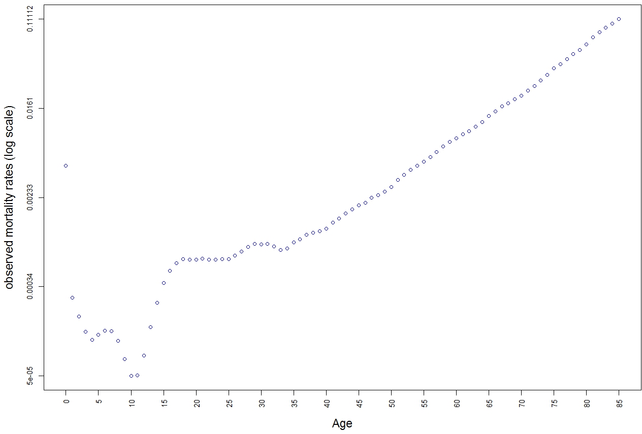
Figure 3: Observed male mortality rates, in logarithmic scale, for the year 2008 in the Sicily Region (Italy).

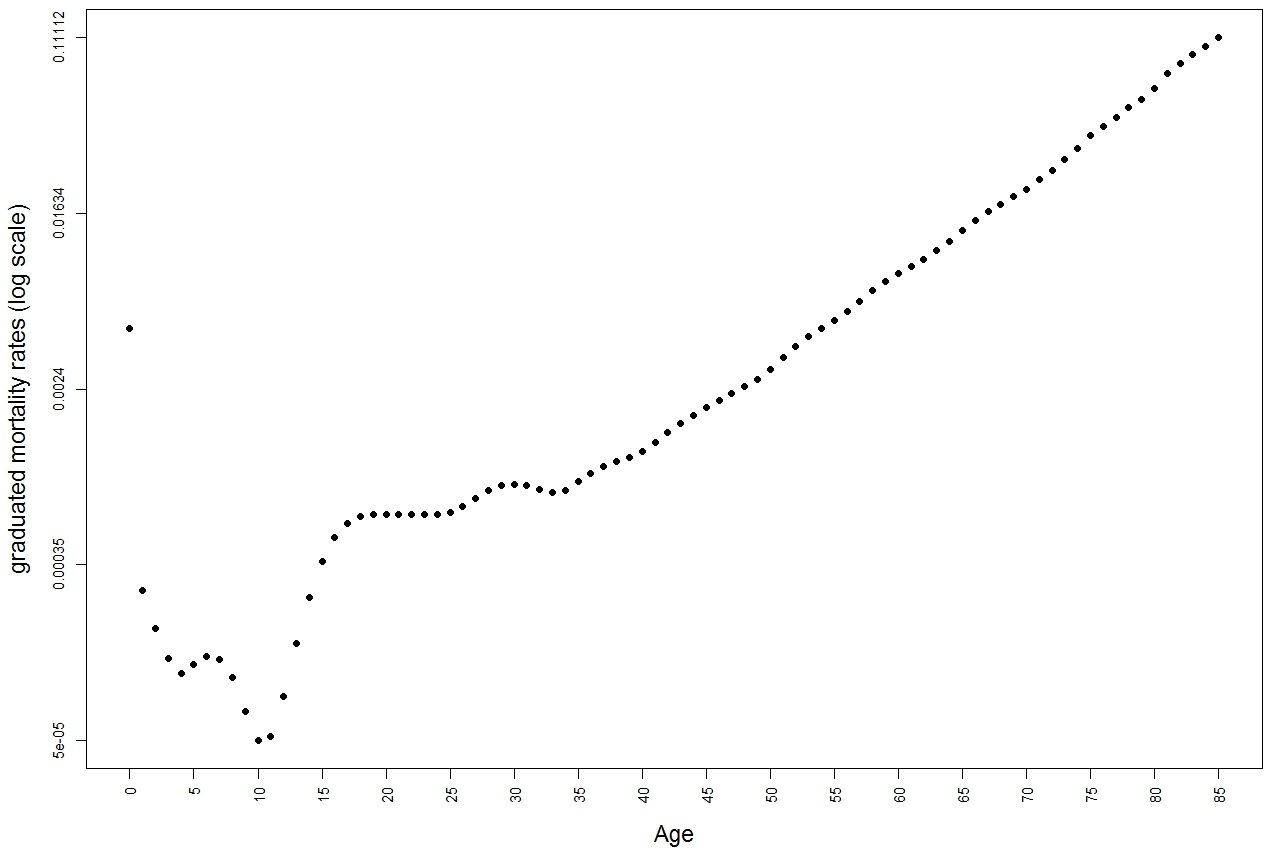
Figure 4: Graduated male mortality rates, in logarithmic scale, for the year 2008 in the Sicily Region (Italy). Graduation is made by the fixed discrete beta kernel estimator in (1) where the bandwidth is estimated by minimizing the cross-validation statistic (7) with residuals defined by (9).

As usual in the graduation literature, a logarithmic scale is used. In both the plots, a small but prominent hump, peaking around 18 years of age, is also visible; this “excess mortality rate”, known in literature as accidental hump, is typically observed especially in males and it is probably due to an increase in a variety of risky activities, the most notable being to obtain a driver’s license. The simultaneous graphical representation of both crude and graduated mortality rates (see Figure 5) is obtained via the command R> plot(resFX1, plottype="obsfit")

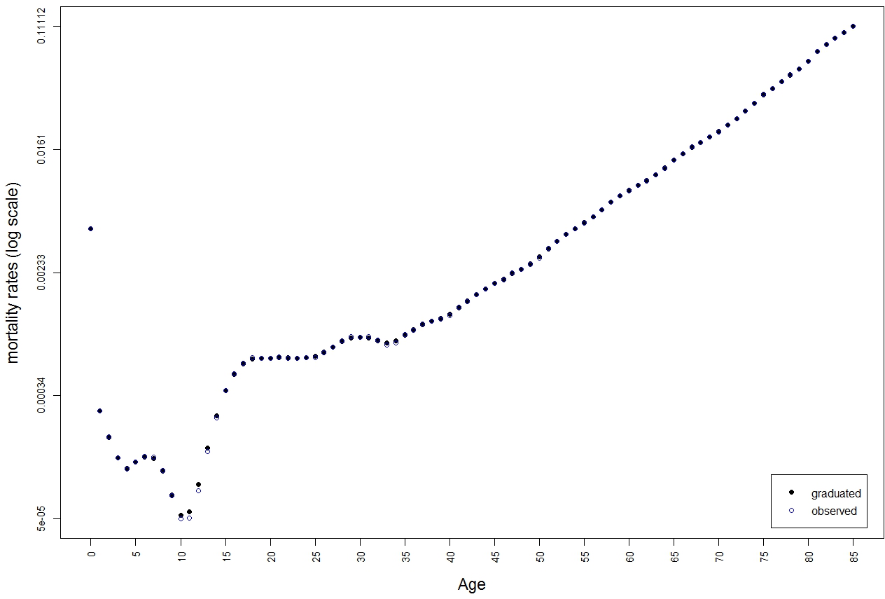
Figure 5: Observed and graduated male mortality rates, in logarithmic scale, for the year 2008 in the Sicily Region (Italy). Graduation is made by the fixed discrete beta kernel estimator in (1) where the bandwidth is estimated by minimizing the cross-validation statistic (7) with residuals defined by (9).

The histogram of the residuals (8), displayed in Figure 6, is obtained by the code R> plot(resFX1, plottype="histres") It could be useful in model diagnostic checking.

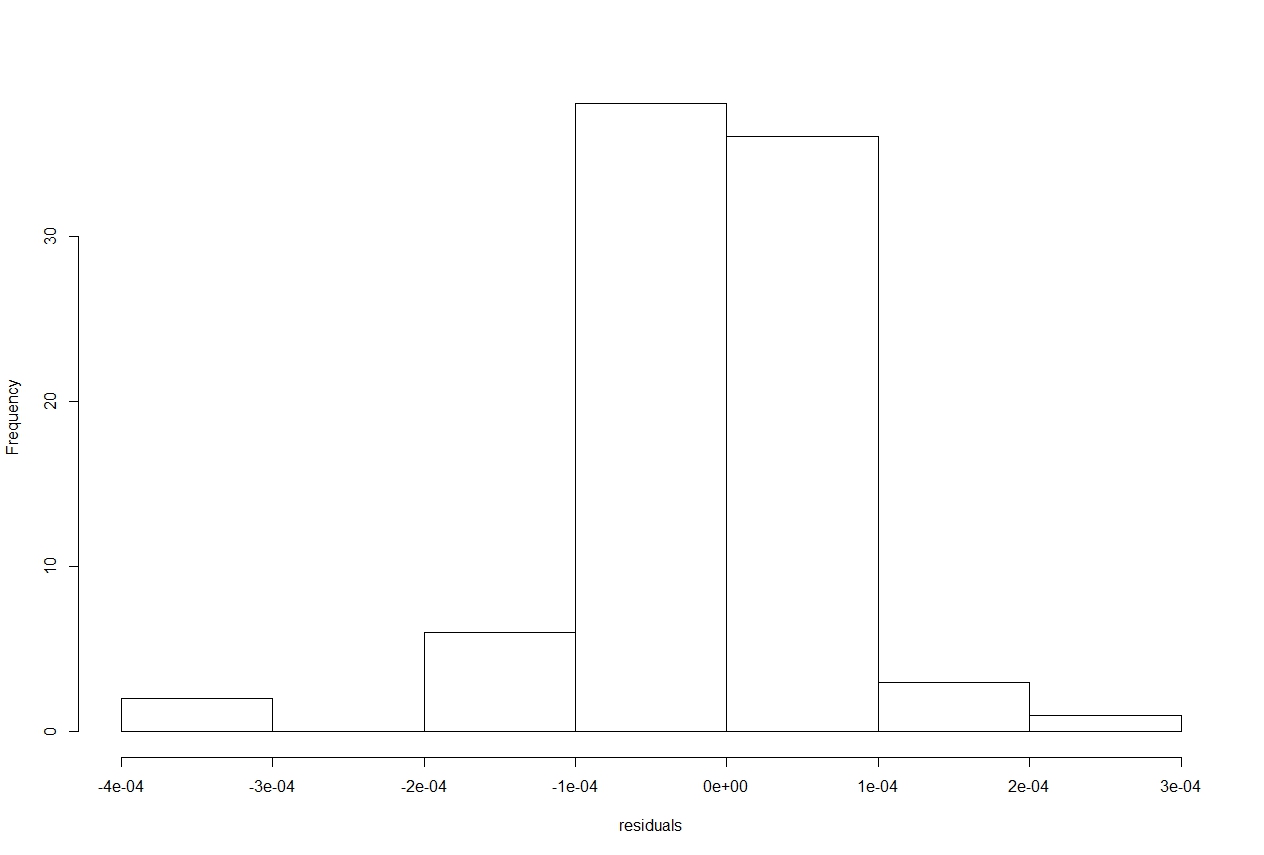
Figure 6: Histogram of the residuals (8) arising from the fitting of the fixed discrete beta kernel estimator in (1) to the mortality rates for the year 2008 in the Sicily Region (Italy). The bandwidth is estimated by minimizing the cross-validation statistic (7) with residuals defined by (9).

The histogram of the proportional residuals (9) can be obtained by specifying plottype="histpropores".

To improve the graphical inspection of the obtained results, pointwise confidence interval can be added to the plot. However, as said in Section 5.3, these intervals require the knowledge of the exposed to risk. Thus, the dbkGrad object needs to be re-created to account for this aspect. The code R> resFX2 <- dbkGrad(obsqx, ex=ex, omega=85, alpha=0.05) R> plot(resFX2, plottype="obsfit", CI=T) produces the plot in Figure 5.

Figure 7: Observed ans graduated male mortality rates, in logarithmic scale, for the year 2008 in the Sicily Region (Italy). Graduation is made by the fixed discrete beta kernel estimator in (1) where the bandwidth is estimated by minimizing the cross-validation statistic (7) with residuals defined by (9). Pointwise 95% confidence intervals, computed as in (11), are also superimposed.

By the argument ex=ex, the exposed to risk are passed to the dbkGrad function. Also in the first row of code, the argument alpha=0.05 – which is the default – specifies the value of $\alpha$ for the pointwise confidence intervals given in (11). In the plot command, the argument plottype="fitted" allows to display only the graduated sequence of points, while CI=T activates the pointwise confidence intervals, with the confidence level specified in the main function above.

Naturally, the user can specify a value for $h$ if, for example, he prefers an higher smoothness. The code R> resFX3 <- dbkGrad(obsqx, ex=ex, omega=85, h=0.01, cvh=F, alpha=0.05) R> plot(resFX3, plottype="obsfit", CI=T) produces the plot in Figure 8 in which, if compared with Figure 5, an higher smothness of the graduated sequence of points can be noted.

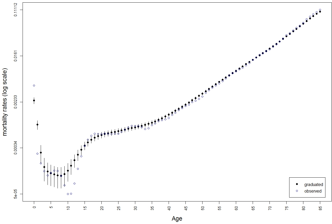
Figure 8: Graduated male mortality rates, in logarithmic scale, for the year 2008 in the Sicily Region (Italy). Graduation is made by the fixed discrete beta kernel estimator in (1) where the bandwidth is manually specified. Pointwise 95% confidence intervals are also superimposed.

This is made possible by the (manual) specification h=0.01, along with the constraint cvh=F which avoids the cross-validation selection of the bandwidth.

So far, the exposed to risk have been only used to define the pointwise confidence intervals. However, as explained in Section 3, they are also useful to take into account the reliability of the data. The code R> plot(resFX3, plottype="exposed") produces the bar plot of the male population at risk displayed in Figure 9.

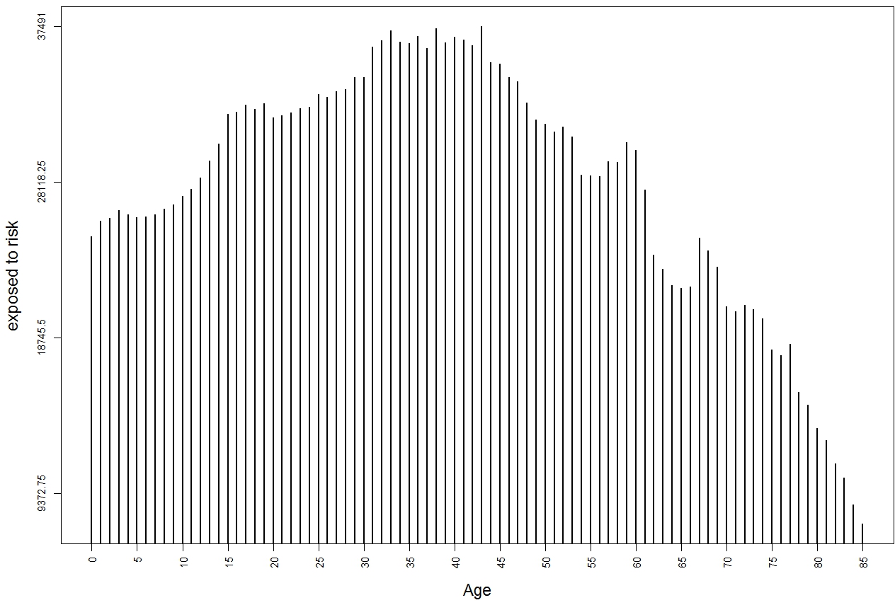
Figure 9: Bar plot of the male exposure for the year 2008 in the Sicily Region.

The great variation in exposure, over the age range, shows the usefulness of an adaptive approach. Note that one offhanded change in exposure is visible in the age ranges 60–62, due to the Second World War. The code R> resEX <- dbkGrad(obsqx, omega=85, ex, bandwidth="EX", s=0.28, + cvres="res", cvh=T, cvs=F, alpha=0.05) It. 0, RSS = 0.000223193, Par. = 0.002 It. 1, RSS = 0.000222536, Par. = 0.00227673 It. 2, RSS = 0.000222489, Par. = 0.00222072 It. 3, RSS = 0.000222489, Par. = 0.00221859 It. 4, RSS = 0.000222489, Par. = 0.00221859 reproduces the scheme followed in Mazza and Punzo (2013) where, the sensitivity parameter is fixed to $s=0.28$, the bandwidth $h$ is selected by minimizing the (conditional) cross-validation statistic $\text{CV}\left(h|s=0.28\right)$ in which the classical residuals in (8) are used via the specification cvres="res". The corresponding graphical representation in Figure 10

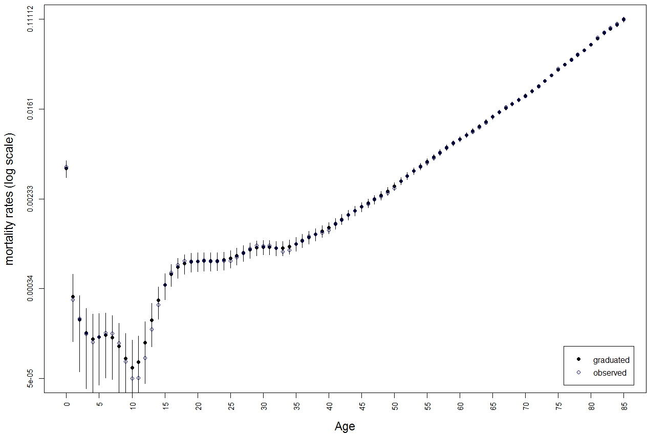
Figure 10: Observed ans graduated male mortality rates, in logarithmic scale, for the year 2008 in the Sicily Region (Italy). Graduation is made by the adaptive discrete beta kernel estimator in (4) where the bandwidth is estimated by minimizing the (conditional) cross-validation statistic $\text{CV}\left(h|s=0.28\right)$ with residuals defined by (8). Pointwise 95% confidence intervals, computed as in (11), are also superimposed.

is obtained via the code R> plot(resEX, plottype="obsfit", CI=T) It is easy to note that the estimated points have a more “graduated” behavior, with respect to the observed ones and to the graduated ones displayed in Figure 7, above all for the ages from 0 to 15.

The code R> resVC <- dbkGrad(obsqx, omega=85, ex, logit=T, bandwidth="VC", + cvh=T, cvs=T, alpha=0.05) R> plot(resVC, plottype="obsfit", CI=T) It. 0, RSS = 0.299308, Par. = 0.002 0.2 It. 1, RSS = 0.29835, Par. = 0.00181587 0.0934201 It. 2, RSS = 0.29803, Par. = 0.0013289 0.0340463 It. 3, RSS = 0.297901, Par. = 0.00114724 0.00665506 It. 4, RSS = 0.297849, Par. = 0.00101142 0 It. 5, RSS = 0.297849, Par. = 0.00101145 0 It. 6, RSS = 0.297849, Par. = 0.00101147 0 It. 7, RSS = 0.297849, Par. = 0.00101148 0 It. 8, RSS = 0.297849, Par. = 0.00101149 0 It. 9, RSS = 0.297849, Par. = 0.00101149 0 It. 10, RSS = 0.297849, Par. = 0.0010115 0 It. 11, RSS = 0.297849, Par. = 0.0010115 0 It. 12, RSS = 0.297849, Par. = 0.0010115 0 It. 13, RSS = 0.297849, Par. = 0.0010115 0 It. 14, RSS = 0.297849, Par. = 0.0010115 0 allows to further show the package flexibility. The graphical result is displayed in Figure 11.

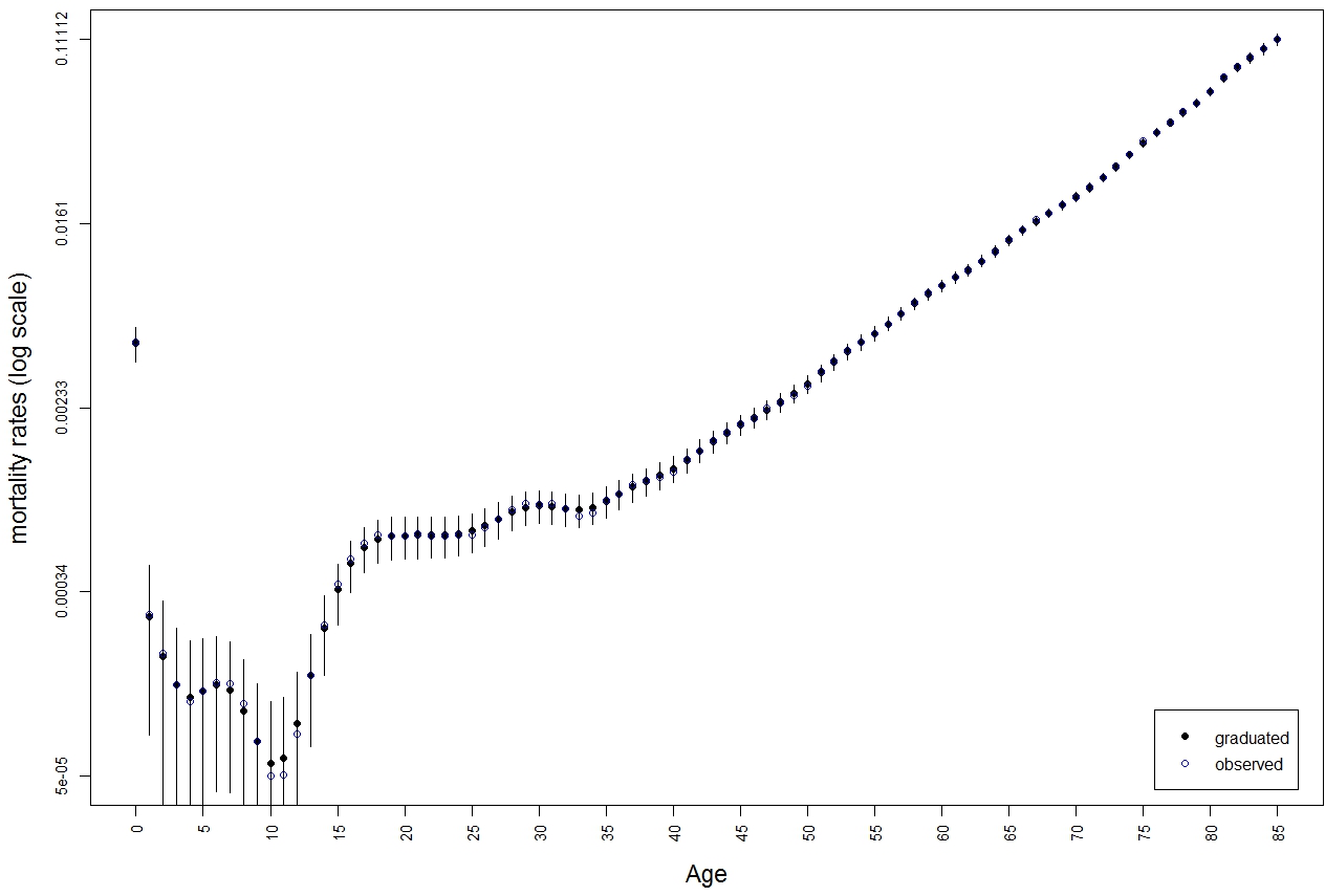
Figure 11: Observed ans graduated male mortality rates, in logarithmic scale, for the year 2008 in the Sicily Region (Italy). Graduation is made by the adaptive discrete beta kernel estimator in (4) where the bandwidth is estimated by minimizing the (joint) cross-validation statistic $\text{CV}\left(h,s\right)$ with residuals defined by (9). A preliminary logit transformation is applied to the rates. Pointwise 95% confidence intervals, computed as in (11), are also superimposed.

In particular, a preliminary logit transformation of the mortality rates is applied (logit=T), as explained in Section 5.2 and, via the specifications cvh=T and cvs=T, both $h$ and $s$ are automatically selected by minimizing the joint cross-validation score $\text{CV}\left(h,s\right)$. An effect of having applied the logit transformation is that, since this time cross-validation selects $s=0$, there is no need of using the adaptive variant of the discrete beta kernel estimator.

Finally, the code R> as.data.frame(resVC) obsqx fitted.values exposed lowerbound upperbound 0 0.00465217 4.583428e-03 24816 3.747432e-03 0.0054194238 1 0.00026728 2.610820e-04 25774 7.551190e-05 0.0004466521 2 0.00017643 1.714462e-04 25950 3.640966e-05 0.0003064828 3 0.00012708 1.269107e-04 26422 2.372682e-05 0.0002300946 4 0.00010655 1.118216e-04 26172 2.192182e-05 0.0002017214 5 0.00011917 1.193277e-04 25976 3.197348e-05 0.0002066819 . . . . . . . . . . . . . . . . . . 80 0.06426613 6.410928e-02 13268 6.138194e-02 0.0668366143 81 0.07523889 7.380717e-02 12551 7.062169e-02 0.0769926510 82 0.08380302 8.287889e-02 11144 7.900452e-02 0.0867532688 83 0.09219433 9.134057e-02 10276 8.661340e-02 0.0960677363 84 0.10101198 1.004669e-01 8676 9.451396e-02 0.1064199097 85 0.11111700 1.110619e-01 7525 1.039997e-01 0.1181241766 summarizes to the user, via a dataframe, the table of all the most important quantities for each age. This may be useful when exporting the results.

7 Conclusions

In this paper we have presented the DBKGrad package for the R environment. This package is specifically conceived for nonparametric graduation of discrete finite functions, such are mortality rates. The package is conceptually simple and easy to use; nevertheless several options are available to the user. He may choose among fixed and adaptive bandwidths, the latter being based, via two different formulations, on the exposed to the risk of dying. Furthermore, the bandwidth and/or a dampening factor may be indicated by the user or chosen by cross-validation; the cross-validation score being minimized may be based on the traditional sum of squared residuals or on an alternative formulation used in the graduation literature, that is the squared proportional residuals. Several plots of either types of residuals, as well as of observed data and of fitted data with confidence intervals, are provided. The package also included an illustrative data set, which contains mortality data for the 2008 male population in the Region of Sicily (Italy). We believe that the DBKGrad package may prove useful to actuaries, demographers, and other social scientists, either as a modeling tool or, if parametric models are to be used, it may still be useful for carrying out a diagnosis of parametric models or simply to examine data.

References

- Bagnato and Punzo (in press) Bagnato L, Punzo A (in press). “Finite Mixtures of Unimodal Beta and Gamma Densities and the -Bumps Algorithm.” Computational Statistics.
- Carroll and Ruppert (1988) Carroll RJ, Ruppert D (1988). Transformation and Weighting in Regression, volume 30. Chapman & Hall, New York.
- Chen (2000) Chen S (2000). “Beta Kernel Smoothers for Regression Curves.” Statistica Sinica, 10(1), 73–91.
- Copas and Haberman (1983) Copas JB, Haberman S (1983). “Non-parametric Graduation Using Kernel Methods.” Journal of the Institute of Actuaries, 110(1), 135–156.
- Cox and Snell (1989) Cox DR, Snell E (1989). Analysis of Binary Data. Chapman & Hall, New York.
- Debòn et al. (2006) Debòn A, Montes F, Sala R (2006). “A Comparison of Nonparametric Methods in the Graduation of Mortality: Application to Data from the Valencia Region (Spain).” International Statistical Review, 74(2), 215–233.
- Elandt-Johnson and Johnson (1980) Elandt-Johnson R, Johnson N (1980). Survival Models and Data Analysis. John Wiley & Sons, Canada.
- Elzhov et al. (2010) Elzhov TV, Mullen KM, Bolker B (2010). \pkgminpack.lm: \proglangR Interface to the Levenberg-Marquardt Nonlinear Least-Squares Algorithm Found in \proglangMINPACK. \proglangR package version 1.1-5. URL http://CRAN.R-project.org/package=minpack.lm.
- Gavin et al. (1993) Gavin J, Haberman S, Verrall R (1993). “Moving Weighted Average Graduation Using Kernel Estimation.” Insurance: Mathematics and Economics, 12(2), 113–126.
- Gavin et al. (1994) Gavin J, Haberman S, Verrall R (1994). “On the Choice of Bandwidth for Kernel Graduation.” Journal of the Institute of Actuaries, 121(1), 119–134.
- Gavin et al. (1995) Gavin J, Haberman S, Verrall R (1995). “Graduation by Kernel and Adaptive Kernel Methods with a Boundary Correction.” Transactions of Society of Actuaries, 47, 173–209.
- Haberman and Renshaw (1996) Haberman S, Renshaw A (1996). “Generalized Linear Models and Actuarial Science.” The Statistician, 45(4), 407–436.
- Härdle (1992) Härdle W (1992). Applied Nonparametric Regression, volume 19 of Econometric Society Monographs. Cambridge University Press, Cambridge.
- Hayfield and Racine (2008) Hayfield T, Racine JS (2008). “Nonparametric Econometrics: The \pkgnp Package.” Journal of Statistical Software, 27(5), 1–32. ISSN 1548-7660. URL http://www.jstatsoft.org/v27/i05.
- Heligman and Pollard (1980) Heligman L, Pollard J (1980). “The Age Pattern of Mortality.” Journal of the Institute of Actuaries, 107(1), 49–80.
- London (1985) London D (1985). Graduation: The Revision of Estimates. Actex publications Abington, Connecticut.
- Mazza and Punzo (2011) Mazza A, Punzo A (2011). “Discrete Beta Kernel Graduation of Age-Specific Demographic Indicators.” In S Ingrassia, R Rocci, M Vichi (eds.), New Perspectives in Statistical Modeling and Data Analysis, volume 42 of Studies in Classification, Data Analysis and Knowledge Organization, pp. 127–134. Springer-Verlag, Berlin-Heidelberg.
- Mazza and Punzo (2013) Mazza A, Punzo A (2013). “Graduation by Adaptive Discrete Beta Kernels.” In A Giusti, G Ritter, M Vichi (eds.), Classification and Data Mining, volume 44 of Studies in Classification, Data Analysis and Knowledge Organization, pp. 77–84. Springer-Verlag, Berlin-Heidelberg.
- Mazza and Punzo (in press) Mazza A, Punzo A (in press). “Using the Variation Coefficient for Adaptive Discrete Beta Kernel Graduation.” In P Giudici, S Ingrassia, M Vichi (eds.), Advances in Statistical Modelling for Data Analysis, Studies in Classification, Data Analysis and Knowledge Organization. Springer-Verlag, Berlin-Heidelberg.
- Moré (1978) Moré J (1978). “The Levenberg-Marquardt Algorithm: Implementation and Theory.” In G Watson (ed.), Numerical Analysis, volume 630 of Lecture Notes in Mathematics, pp. 104–116. Springer-Verlag, Berlin-Heidelberg.
- Peristera and Kostaki (2005) Peristera P, Kostaki A (2005). “An Evaluation of the Performance of Kernel Estimators for Graduating Mortality Data.” Journal of Population Research, 22(2), 185–197.
- Punzo (2010) Punzo A (2010). “Discrete Beta-type Models.” In H Locarek-Junge, C Weihs (eds.), Classification as a Tool for Research, volume 40 of Studies in Classification, Data Analysis and Knowledge Organization, pp. 253–261. Springer-Verlag, Berlin-Heidelberg.
- Punzo and Zini (2012) Punzo A, Zini A (2012). “Discrete Approximations of Continuous and Mixed Measures on a Compact Interval.” Statistical Papers, 53(3), 563–575.
- \proglangR Development Core Team (2012) \proglangR Development Core Team (2012). \proglangR: A Language and Environment for Statistical Computing. \proglangR Foundation for Statistical Computing, Vienna, Austria. ISBN 3-900051-07-0, URL http://www.R-project.org/.
- Renshaw (1991) Renshaw A (1991). “Actuarial Graduation Practice and Generalized Linear and Non-Linear Models.” Journal of the Institute of Actuaries, 118(2), 295–312.
- Stone (1974) Stone M (1974). “Cross-Validatory Choice and Assessment of Statistical Predictions.” Journal of the Royal Statistical Society: Series B, 36(1), 111–147.