Abstract

The cargo motion in living cells transported by two species of motor protein with different intrinsic directionality is discussed in this study. Similar to single motor movement, cargo steps forward and backward along microtubule stochastically. Recent experiments found that, cargo transportation by two motor species has a memory, it does not change its direction as frequently as expected, which means that its forward and backward step rates depends on its previous motion trajectory. By assuming cargo has only the least memory, i.e. its step direction depends only on the direction of its last step, two cases of cargo motion are detailed analyzed in this study: (I) cargo motion under constant external load; and (II) cargo motion in one fixed optical trap. Due to the existence of memory, for the first case, cargo can keep moving in the same direction for a long distance. For the second case, the cargo will oscillate in the trap. The oscillation period decreases and the oscillation amplitude increases with the motor forward step rates, but both of them decrease with the trap stiffness. The most likely location of cargo, where the probability of finding the oscillated cargo is maximum, may be the same as or may be different with the trap center, which depends on the step rates of the two motor species. Meanwhile, if motors are robust, i.e. their forward to backward step rate ratios are high, there may be two such most likely locations, located on the two sides of the trap center respectively. The probability of finding cargo in given location, the probability of cargo in forward/backward motion state, and various mean first passage times of cargo to give location or given state are also analyzed.

Introduction

Motility is one of the basic properties of living cells, in which cargos, including organelles and vesicles, are usually transported by cooperation of various motor proteins [1, 2], such as the plus-end directed kinesin and minus-directed dynein [3, 4, 5]. Experiments found that, using the energy released in ATP hydrolysis [6, 7, 8, 9], these motors can move processively along microtubule with step size 8 nm and in hand-over-hand manner [10, 11, 12].

Although numerous experimental and theoretical studies have been done to understand this cargo transportation process, so far the mechanism of which is not fully clear. In [13], one basic model is presented by assuming cargo is transported by only one motor species and all the motors share the external load equally. Then in [14], one more realistic tug-of-war model is designed, in which the cargo is assumed to be transported by two motor species with opposite intrinsic directionality, and motors can reverse their motion direction under large external load. According to some experimental phenomena this tug-of-war model seems reasonable [15, 16]. In either of the models given in [13, 14], the only interaction among different motors is that, motors from the same species share load equally and motors from different species act as load to each other. In [17, 18, 19], some complicated models are presented, in which interactions among motors are described by linear springs. Recent experiments found that the tug-of-war model might not be reasonable enough to explain some experimental phenomena, so several new models are designed to try to understand the mechanism of cargo motion by multiple motors [20, 21, 22, 23, 24, 25, 26]. Finally, more discussion about cargo transportation in cells can be found in [27, 28, 29, 30, 31, 32, 33, 34, 35].

In recent experiment [36], by measuring cargo dynamics in optical trap, Leidel et al. found cargo motion along microtubule has memory. Cargo is more likely to resume motion in the same direction rather than the opposite one. This finding implies that, cargo location in the next time depends not only on its present location but also on how it reaches the present location. The behavior of cargo depends on its motion trajectory, which is different from the assumptions in previous models. In this study, one model for cargo motion with memory will be presented. But for simplicity, we assume that the cargo has only a little memory, it can only remember the motion direction in its last step. The description and theoretical analysis of the model with memory will be first given in the next section, and then corresponding results will be presented in the following section. Results will be summarized in the final section.

Model for cargo motion with memory

In this study, the cargo is assumed to be tightly bound by two motor species: plus-end (or forward) motors and minus-end (or backward) motors. The forward and backward step rates of each plus-end motor are $u$ and $w$, and the forward and backward step rates of each minus-end motor are $f$ and $b$. Obviously $u\gg w$ but $b\gg f$ when the external load is low, since the intrinsic directionalities of the two motor species are opposite to each other, and the intrinsic motion direction of plus-end motor is plus-end directed (i.e. to the plus-end of microtubule), but the intrinsic motion direction of minus-end motor is minus-end directed (i.e. to the minus-end of microtubule). By assuming that all motors from the same motor species share the load equally, we only need to discuss the simplest cases in which the cargo is transported by only one plus-end motor and one minus-end motor. For example, if there are $k$ plus-end motors, the total external load is $F_{c}$, the forward and backward step rates of one single plus-end motor are $u_{c}$ and $w_{c}$, and the motor step size is $l_{c}$. Then these $k$ plus-end motors can be effectively replaced by one single plus-end motor with load $F=F_{c}/k$, step rates $u=ku_{c}$ and $w=kw_{c}$, and step size $l_{0}=l_{c}/k$. Since the experiments in [36] showed that, the number of motors moving the cargo is usually the same in both directions, this study also assumes the step sizes of the plus-end motor and minus-end motor are the same (note, the step size of single plus-end motor kinesin and step size of single minus-end motor dynein are the same $l_{0}\approx 8$ nm [2, 9, 12]).

This study will mainly discuss two special cases: (I) Cargo moves under constant external load. In vitro, this constant load may be applied by one feedback optical trap, or In vivo, this constant load may be from the viscous environment with invariable drag coefficient. (II) Cargo moves in one fixed optical trap, this case is easy to be performed experimentally, and so the corresponding theoretical results are easy to be verified.

Cargo Motion under constant load

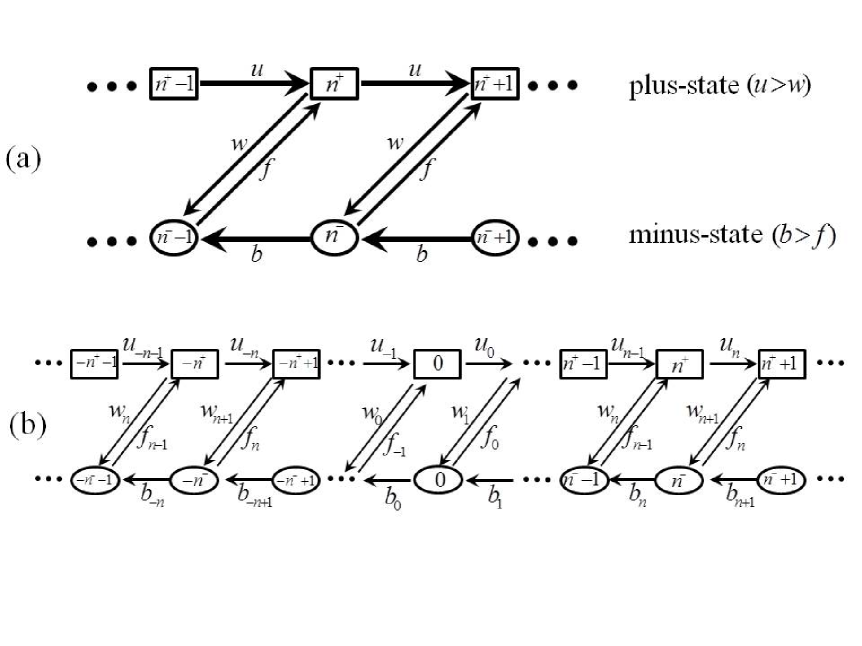
Figure 1: Schematic depiction of the model discussed in this study to explain the cargo motion with memory. (a) is for cargo motion under constant load, and (b) is for cargo motion in one fixed optical trap. At any location $n$, the cargo may be in two different states, plus-state $n^{+}$ and minus-state $n^{-}$. Cargo in plus-state $n^{+}$ means it reaches location $n$ from location $n-1$, while cargo in minus-state means it is from location $n+1$. For a cargo in plus-state $n^{+}$, its forward and backward step rates are $u$ and $w$ respectively. But for a cargo in minus-state $n^{-}$, it has different step rates $f$ and $b$. For the constant load cases (a), $u>w$ and $b>f$ mean that, if the cargo is in plus-state $n^{+}$ it will be more likely to move forward to location $n+1$. Otherwise, it will be more likely to move backward to location $n-1$.

For the sake of convenience, the cargo is said to be in plus-state $n^{+}$ if it reached its present location $n$ by one forward step from location $n-1$. Similarly, the cargo is said to be in minus-state $n^{-}$ if its previous step is minus-end directed, see Fig. 1(a) for the schematic depiction. In plus-state, the forward step rate is higher than backward step rate $u>w$, but in minus-state the forward step rate is lower than backward step rate $f<b$. So in plus-state, the cargo is more likely to move forward, but in minus-state, the cargo will be more likely to move backward. For example, for a cargo in location $n$, if its previous step is plus-end directed, from either plus-state $n^{+}-1$ or minus-state $n^{-}-1$ to location $n$, then in the next step the cargo will be more likely to move to location $n+1$ (plus-state $n^{+}+1$), since the cargo is now in plus-state $n^{+}$ and its forward step rate $u$ is higher than its backward step rate $w$. On the contrary, if it got to its present location $n$ from location $n+1$ (either from plus-state $n^{+}+1$ or from minus-state $n_{-}+1$), then in the next step the cargo will be more likely to move to location $n-1$ (minus-state $n^{-}-1$), since the cargo is now in minus-state $n^{-}$ and its backward step rate $b$ is higher than its forward step rate $f$. This behavior means that the cargo can remember its motion direction of its last step.

Let $p,\rho$ be probabilities of cargo in plus-state and minus-state respectively, then

$$dp/dt=f\rho-wp=-d\rho/dt.$$ (1)

Using the normalization condition $p+\rho=1$, its steady state solution can be obtained as follows

$$p=f/(f+w),\quad\rho=w/(f+w).$$ (2)

Let $U_{eff}=up+f\rho$, $W_{eff}=wp+b\rho$, then the mean velocity of cargo can be obtained as follows

$$V=(U_{eff}-W_{eff})l_{0}=[(u-w)p+(f-b)\rho]l_{0}=(uf-wb)l_{0}/(f+w),$$ (3)

where $l_{0}$ is the step size of cargo. The probabilities that cargo steps forward and backward are then

$$p_{+}=\frac{U_{eff}}{U_{eff}+W_{eff}}=\frac{f(u+w)}{f(u+w)+w(f+b)},$$ (4)

$$p_{-}=1-p_{+}=\frac{w(f+b)}{f(u+w)+w(f+b)}.$$

Finally, the external load $F$ dependence of rate $u,w,f,b$ can be given by the following Bell approximation [37, 38, 39, 40],

$$u=u_{0}e^{-\epsilon_{0}Fl_{0}/k_{B}T},\quad w=w_{0}e^{(1-\epsilon_{0})Fl_{0}/k_{B}T},\quad f=f_{0}e^{-\epsilon_{1}Fl_{0}/k_{B}T},\quad b=b_{0}e^{(1-\epsilon_{1})Fl_{0}/k_{B}T}.$$ (5)

Where $\epsilon_{0}$ and $\epsilon_{1}$ are load distribution factors for the plus-end motor and minus-end motor, respectively. $k_{B}$ is Boltzmann constant, and $T$ is the absolute temperature.

Cargo Motion in one fixed optical trap

This special case is schematically depicted in Fig. 1(b). For convenience, the center of optical trap is assumed to be fixed at location $0$. For this case, the potential of cargo depends on its location $n$. The potential difference between location $n$ and location $n+1$ is $\Delta G_{n}=\kappa[(n+1)l_{0}]^{2}/2-\kappa(nl_{0})^{2}/2=\kappa(n+1/2)l_{0}^{2}$. Similar as in [19], at location $n$, the forward and backward step rates $u_{n}$ and $w_{n}$ of cargo in plus-state, as well as the step rates $f_{n}$ and $b_{n}$ of cargo in minus-state, can be obtained as follows,

$$u_{n}=ue^{-\epsilon_{0}\Delta G_{n}/k_{B}T},\quad w_{n}=we^{(1-\epsilon_{0})\Delta G_{n-1}/k_{B}T},\quad f_{n}=fe^{-\epsilon_{1}\Delta G_{n}/k_{B}T},\quad b_{n}=be^{(1-\epsilon_{1})\Delta G_{n-1}/k_{B}T}.$$ (6)

Where $u,w,f,b$ are cargo step rates when there is no optical trap and any other external load, which satisfy $u\gg w,b\gg f$. For simplicity, this study assumes that $\epsilon_{0}$, $\epsilon_{1}$ are independent of cargo location $n$.

Let $p_{n},\rho_{n}$ be the probabilities of finding cargo in plus-state $n^{+}$ and minus-state $n^{-}$, respectively. One can easily show $p_{n},\rho_{n}$ are governed by the following equations

$$dp_{n}/dt=u_{n-1}p_{n-1}+f_{n-1}\rho_{n-1}-(u_{n}+w_{n})p_{n},$$ (7a)

$$d\rho_{n}/dt=w_{n+1}p_{n+1}+b_{n+1}\rho_{n+1}-(f_{n}+b_{n})\rho_{n}.$$ (7b)

The steady state solution of Eqs. (7a, 7b) are as follows (for details see Sec. A of the supplemental materials)

$$p_{n}=\left[\prod_{k=0}^{n-1}\left(\frac{(f_{k}+b_{k})u_{k}}{(u_{k+1}+w_{k+1})b_{k}}\right)\right]p_{0},\quad\textrm{for\ }n\geq 1,$$ (8a)

$$p_{n}=\left[\prod_{k=n+1}^{0}\left(\frac{(u_{k}+w_{k})b_{k-1}}{(f_{k-1}+b_{k-1})u_{k-1}}\right)\right]p_{0},\quad\textrm{for\ }n\leq-1,$$ (8b)

$$\rho_{n}=\frac{u_{n}}{b_{n}}p_{n}=\frac{u_{n}}{b_{n}}\left[\prod_{k=0}^{n-1}\left(\frac{(f_{k}+b_{k})u_{k}}{(u_{k+1}+w_{k+1})b_{k}}\right)\right]p_{0},\quad\textrm{for\ }n\geq 1,$$ (8c)

$$\rho_{n}=\frac{u_{n}}{b_{n}}p_{n}=\frac{u_{n}}{b_{n}}\left[\prod_{k=n+1}^{0}\left(\frac{(u_{k}+w_{k})b_{k-1}}{(f_{k-1}+b_{k-1})u_{k-1}}\right)\right]p_{0},\quad\textrm{for\ }n\leq-1,$$ (8d)

$$\rho_{0}=\frac{u_{0}}{b_{0}}p_{0}.$$ (8e)

Where $p_{0}$ can be obtained by the normalization condition $\sum_{n=-\infty}^{+\infty}(p_{n}+\rho_{n})=1$.

The probability of finding cargo in plus-state is $p=\sum_{n=-\infty}^{+\infty}p_{n}$, and the probability of finding cargo in minus-state is $\rho=\sum_{n=-\infty}^{+\infty}\rho_{n}$. The mean locations of cargo in plus-state and in minus-state are

$$\langle n^{+}\rangle=\sum_{n=-\infty}^{+\infty}np_{n}/p,\quad\langle n^{-}\rangle=\sum_{n=-\infty}^{+\infty}n\rho_{n}/\rho,$$ (9a)

respectively. The mean location of cargo is

$$\langle n\rangle=\sum_{n=-\infty}^{+\infty}n(p_{n}+\rho_{n})=p\langle n^{+}\rangle+\rho\langle n^{-}\rangle.$$ (10)

Specially, for the symmetric cases $u=b,w=f$, i.e. the cargo is transported by two motors with the same step rates but different intrinsic directionality, one can verify that $\rho_{n}=p_{-n}$ and consequently $\rho=p,\langle n^{-}\rangle=-\langle n^{+}\rangle,\langle n\rangle=0$.

The external load dependence of rates $u_{n},w_{n},f_{n},b_{n}$ [see Eq. (6)] means that, for a cargo towed by two motors in one fixed optical trap there are two critical values of the cargo location $n$,

$$n_{c+}=\left\lceil\frac{k_{B}T}{\kappa l_{0}^{2}}\ln\frac{u}{w}+\frac{1}{2}-\epsilon_{0}\right\rceil,\quad n_{c-}=\left\lfloor\frac{k_{B}T}{\kappa l_{0}^{2}}\ln\frac{f}{b}+\frac{1}{2}-\epsilon_{1}\right\rfloor,$$ (11)

where $\lceil x\rceil$ is the smallest integer number which is not less than $x$, $\lfloor x\rfloor$ is the biggest integer number which is not bigger than $x$. The step rates of plus-end motor satisfy $u_{n}>w_{n}$ for $n<n_{c+}$, and $u_{n}\leq w_{n}$ for $n\geq n_{c+}$. Similarly, the step rates of minus-end motor satisfy $b_{n}>f_{n}$ for $n>n_{c-}$, and $b_{n}\leq f_{n}$ for $n\leq n_{c-}$. The intrinsic directionality of plus-end motor ($u\gg w$) implies $n_{c+}>0$, and the intrinsic directionality of minus-end motor ($b\gg f$) implies $n_{c-}<0$. Generally, the critical values $n_{c+}$ and $n_{c-}$ are different with the mean locations $\langle n^{+}\rangle$ and $\langle n^{-}\rangle$.

In the following of this section, various mean first passage time (MFPT) problems about the cargo motion in fixed optical trap will be discussed.

Mean first passage time to one of the plus-state

Let $t_{n}^{l}$ and $\tau_{n}^{l}$ be MFPTs of cargo from plus-state $n^{+}$ and minus-state $n^{-}$ to plus-state $l^{+}$ respectively, then $t_{n}^{l}$ and $\tau_{n}^{l}$ satisfy [41, 42]

$$w_{n}\tau_{n-1}^{l}-(u_{n}+w_{n})t_{n}^{l}+u_{n}t_{n+1}^{l}=-1,\quad\textrm{for\ }n\neq l,$$ (12a)

$$b_{n}\tau_{n-1}^{l}-(f_{n}+b_{n})\tau_{n}^{l}+f_{n}t_{n+1}^{l}=-1,$$ (12b)

with one boundary condition $t_{l}^{l}=0$.

From Eq. (12a) one can easily get

$$\tau_{n-1}^{l}=\frac{u_{n}+w_{n}}{w_{n}}t_{n}^{l}-\frac{u_{n}}{w_{n}}t_{n+1}^{l}-\frac{1}{w_{n}},\quad\textrm{for\ }n\neq l.$$ (13)

Substituting (13) into (12b), one obtains

$$b_{n}\left[\frac{u_{n}+w_{n}}{w_{n}}t_{n}^{l}-\frac{u_{n}}{w_{n}}t_{n+1}^{l}-\frac{1}{w_{n}}\right]-(f_{n}+b_{n})\left[\frac{u_{n+1}+w_{n+1}}{w_{n+1}}t_{n+1}^{l}-\frac{u_{n+1}}{w_{n+1}}t_{n+2}^{l}-\frac{1}{w_{n+1}}\right]+f_{n}t_{n+1}^{l}=-1,$$ (14)

i.e.

$$B_{n}t_{n}^{l}-(B_{n}+F_{n})t_{n+1}^{l}+F_{n}t_{n+2}^{l}=C_{n},$$ (15)

where

$$B_{n}=\frac{(u_{n}+w_{n})b_{n}}{w_{n}},\quad F_{n}=\frac{(f_{n}+b_{n})u_{n+1}}{w_{n+1}},\quad C_{n}=\frac{b_{n}}{w_{n}}-\frac{f_{n}+b_{n}}{w_{n+1}}-1.$$ (16)

Note, Eqs. (14, 15) are established for $n\neq l-1,l$.

Meanwhile, from Eq. (12b) one can get

$$t_{n+1}^{l}=\frac{f_{n}+b_{n}}{f_{n}}\tau_{n}^{l}-\frac{b_{n}}{f_{n}}\tau_{n-1}^{l}-\frac{1}{f_{n}},$$ (17)

and then by substituting Eq. (17) into Eq. (12a) one obtains

$$w_{n}\tau_{n-1}^{l}-(u_{n}+w_{n})\left[\frac{f_{n-1}+b_{n-1}}{f_{n-1}}\tau_{n-1}^{l}-\frac{b_{n-1}}{f_{n-1}}\tau_{n-2}^{l}-\frac{1}{f_{n-1}}\right]+u_{n}\left[\frac{f_{n}+b_{n}}{f_{n}}\tau_{n}^{l}-\frac{b_{n}}{f_{n}}\tau_{n-1}^{l}-\frac{1}{f_{n}}\right]=-1,$$ (18)

i.e.

$$\hat{B}_{n}\tau_{n-2}^{l}-(\hat{B}_{n}+\hat{F}_{n})\tau_{n-1}^{l}+\hat{F}_{n}\tau_{n}^{l}=\hat{C}_{n},$$ (19)

where

$$\hat{B}_{n}=\frac{(u_{n}+w_{n})b_{n-1}}{f_{n-1}},\quad\hat{F}_{n}=\frac{(f_{n}+b_{n})u_{n}}{f_{n}},\quad\hat{C}_{n}=\frac{u_{n}}{f_{n}}-\frac{u_{n}+w_{n}}{f_{n-1}}-1.$$ (20)

Eqs. (18, 19) are established for $n\neq l$.

The procedure of getting MFPTs $t_{n}^{l},\tau_{n}^{l}$ is as follows. (1) Getting $t_{n}^{l}$ for $n\leq l-1$ by Eq. (15) and boundary condition $t_{l}^{l}=0$ (see Sec. B of the supplemental materials). (2) Getting $\tau_{n}^{l}$ for $n\leq l-2$ by Eq. (13). (3) Getting $\tau_{l-1}^{l}$ from the special case of Eq. (12b), i.e. $b_{l-1}\tau_{l-2}^{l}-(f_{l-1}+b_{l-1})\tau_{l-1}^{l}=-1$. (4) Getting $\tau_{n}^{l}$ for $n\geq l$ by Eq. (19) and boundary value $\tau_{l-1}^{l}$ obtained in (3) (see Sec. C of the supplemental materials). (5) Getting $t_{n}^{l}$ for $n\geq l+1$ by Eq. (17). This procedure can be summarized as follows

$$\xLongrightarrow[t_{l}^{l}=0]{\textrm{Eq. (\ref{eq19})}}t_{n}^{l}(n\leq l-1)\xLongrightarrow{\textrm{Eq. (\ref{eq17})}}\tau_{n}^{l}(n\leq l-2)\xLongrightarrow[n=l-1]{\textrm{Eq. (\ref{eq16b})}}\tau_{l-1}^{l}\xLongrightarrow{\textrm{Eq. (\ref{eq23})}}\tau_{n}^{l}(n\geq l)\xLongrightarrow{\textrm{Eq. (\ref{eq21})}}t_{n}^{l}(n\geq l+1).$$ (21)

Mean first passage time to one of the minus-state

Let $\bar{t}_{n}^{l}$ and $\bar{\tau}_{n}^{l}$ be the MFPTs of cargo from plus-state $n^{+}$ and minus-state $n^{-}$ to minus-state $l^{-}$, respectively. Similar as the discussion in Sec. Mean first passage time to one of the plus-state, the MFPTs $\bar{t}_{n}^{l}$ and $\bar{\tau}_{n}^{l}$ satisfy the following equations

$$w_{n}\bar{\tau}_{n-1}^{l}-(u_{n}+w_{n})\bar{t}_{n}^{l}+u_{n}\bar{t}_{n+1}^{l}=-1,$$ (22a)

$$b_{n}\bar{\tau}_{n-1}^{l}-(f_{n}+b_{n})\bar{\tau}_{n}^{l}+f_{n}\bar{t}_{n+1}^{l}=-1,\quad\textrm{for\ }n\neq l,$$ (22b)

with one boundary condition $\bar{\tau}_{l}^{l}=0$. From Eq. (22a) one can easily get

$$\bar{\tau}_{n-1}^{l}=\frac{u_{n}+w_{n}}{w_{n}}\bar{t}_{n}^{l}-\frac{u_{n}}{w_{n}}\bar{t}_{n+1}^{l}-\frac{1}{w_{n}}.$$ (23)

Substituting (23) into (22b), one obtains

$$b_{n}\left[\frac{u_{n}+w_{n}}{w_{n}}\bar{t}_{n}^{l}-\frac{u_{n}}{w_{n}}\bar{t}_{n+1}^{l}-\frac{1}{w_{n}}\right]-(f_{n}+b_{n})\left[\frac{u_{n+1}+w_{n+1}}{w_{n+1}}\bar{t}_{n+1}^{l}-\frac{u_{n+1}}{w_{n+1}}\bar{t}_{n+2}^{l}-\frac{1}{w_{n+1}}\right]+f_{n}\bar{t}_{n+1}^{l}=-1,$$ (24)

i.e.

$$B_{n}\bar{t}_{n}^{l}-(B_{n}+F_{n})\bar{t}_{n+1}^{l}+F_{n}\bar{t}_{n+2}^{l}=C_{n},$$ (25)

with $B_{n},F_{n},C_{n}$ given by Eq. (16). Note, Eqs. (24, 25) are established for $n\neq l$.

Meanwhile, from Eq. (22b) one can get

$$\bar{t}_{n+1}^{l}=\frac{f_{n}+b_{n}}{f_{n}}\bar{\tau}_{n}^{l}-\frac{b_{n}}{f_{n}}\bar{\tau}_{n-1}^{l}-\frac{1}{f_{n}},\quad\textrm{for\ }n\neq l,$$ (26)

and then by substituting Eq. (26) into Eq. (22a) one obtains

$$w_{n}\bar{\tau}_{n-1}^{l}-(u_{n}+w_{n})\left[\frac{f_{n-1}+b_{n-1}}{f_{n-1}}\bar{\tau}_{n-1}^{l}-\frac{b_{n-1}}{f_{n-1}}\bar{\tau}_{n-2}^{l}-\frac{1}{f_{n-1}}\right]+u_{n}\left[\frac{f_{n}+b_{n}}{f_{n}}\bar{\tau}_{n}^{l}-\frac{b_{n}}{f_{n}}\bar{\tau}_{n-1}^{l}-\frac{1}{f_{n}}\right]=-1,$$ (27)

i.e.

$$\hat{B}_{n}\bar{\tau}_{n-2}^{l}-(\hat{B}_{n}+\hat{F}_{n})\bar{\tau}_{n-1}^{l}+\hat{F}_{n}\bar{\tau}_{n}^{l}=\hat{C}_{n},$$ (28)

with $\hat{B}_{n},\hat{F}_{n},\hat{C}_{n}$ given by Eq. (20). Eqs. (27, 28) are established for $n\neq l,l+1$.

The procedure of getting MFPTs $\bar{t}_{n}^{l},\bar{\tau}_{n}^{l}$ is as follows. (1) Getting $\bar{\tau}_{n}^{l}$ for $n\geq l+1$ by Eq. (28) and boundary condition $\bar{\tau}_{l}^{l}=0$ (see Sec. D of the supplemental materials). (2) Getting $\bar{t}_{n}^{l}$ for $n\geq l+2$ by Eq. (26). (3) Getting $\bar{t}_{l+1}^{l}$ from the special case of Eq. (22a), i.e. $-(u_{l+1}+w_{l+1})\bar{t}_{l+1}^{l}+u_{l+1}\bar{t}_{l+2}^{l}=-1$, (4) Getting $\bar{t}_{n}^{l}$ for $n\leq l$ by Eq. (25) with boundary value $\bar{t}_{l+1}$ obtained in (3) (see Sec. E of the supplemental materials). (5) Getting $\bar{\tau}_{n}^{l}$ for $n\leq l-1$ by Eq. (23). This procedure can be summarized as follows

$$\xLongrightarrow[\bar{\tau}_{l}^{l}=0]{\textrm{Eq. (\ref{eq32})}}\bar{\tau}_{n}^{l}(n\geq l+1)\xLongrightarrow{\textrm{Eq. (\ref{eq30})}}\bar{t}_{n}^{l}(n\geq l+2)\xLongrightarrow[n=l+1]{\textrm{Eq. (\ref{eq25a})}}\bar{t}_{l+1}^{l}\xLongrightarrow{\textrm{Eq. (\ref{eq28})}}\bar{t}_{n}^{l}(n\leq l)\xLongrightarrow{\textrm{Eq. (\ref{eq26})}}\bar{\tau}_{n}^{l}(n\leq l-1).$$ (29)

Mean first passage time to one given location

Let ${\cal T}_{s}^{l}$ be the MFPT of cargo from state $s$ to location $l$ (either plus-state $l^{+}$ or minus-state $l^{-}$), then one can easily show that

$${\cal T}_{s}^{l}=\left\{\begin{array}[]{llll}t_{k}^{l},&\textrm{for\ }s=k^{+}&\textrm{and}&k<l,\cr\tau_{k}^{l},&\textrm{for\ }s=k^{-}&\textrm{and}&k<l,\cr\bar{t}_{k}^{l},&\textrm{for\ }s=k^{+}&\textrm{and}&k>l,\cr\bar{\tau}_{k}^{l},&\textrm{for\ }s=k^{-}&\textrm{and}&k>l.\end{array}\right.$$ (30)

It is to say that if $k<l$, a cargo located at $k$ will first reach plus-state $l^{+}$ before reaching minus-state $l^{-}$. On the contrary, if $k>l$, it will first reach minus-state $l^{-}$. Finally, the mean oscillation period $T$ of cargo in fixed optical trap can be approximated as follows

$$T\approx\tau_{0}^{0}+\bar{t}_{0}^{0},$$ (31)

see Sec. F of the supplemental materials for its expression.

Results

For cargo motion under no external load, Monte Carlo simulations show that, if the cargo is transported by two symmetric motors, i.e., the plus-end motor and the minus-end motor have the same step rates, $u=b,w=f$, the cargo will oscillate [Fig. 2(a)]. While for the asymmetric cases, the cargo has non-zero mean velocity [see Fig. 2(b)]. On the other hand, if the cargo is put into one fixed optical trap, and transported by two symmetric motors, it will oscillate around the trap center with relatively high frequency [Fig. 2(c)]. Meanwhile, if the trapped cargo is transported by two asymmetric motors, it will also oscillate but its oscillation center may be different with the trap center [Fig. 2(d)]. Both Monte Carlo simulations and theoretical calculations show that, for a cargo transported by two symmetric motors and put in one optical trap, its oscillation period $T$ decreases with trap stiffness $\kappa$, motor forward step rates $u=b$, and motor backward step rates $w=f$ [Fig. 3(a-c)]. Its oscillation amplitude increases with the motor forward step rates $u=b$, but decreases with both the motor backward step rates $u=b$ and the trap stiffness $\kappa$, since high backward step rates and high trap stiffness will prohibit the cargo from moving too far from the trap center [Fig. 3(d-f)].

Let

$$p=\sum_{n=-\infty}^{\infty}p_{n},\quad\rho=\sum_{n=-\infty}^{\infty}\rho_{n},\quad P_{+}=\sum_{n>0}(p_{n}+\rho_{n}),\quad P_{-}=\sum_{n<0}(p_{n}+\rho_{n}).$$ (32)

Then $p$ is the probability of finding cargo in plus-state, $P_{+}$ is the probability that cargo location $n>0$ (the center of optical trap is assumed to be at location 0). The meanings of $\rho$ and $P_{-}$ are similar. Both Monte Carlo simulations and theoretical calculations show that, for a cargo transported by two symmetric motors, the ratios $p/\rho$ and $P_{+}/P_{-}$ are always one, and they do not change with trap stiffness $\kappa$, forward step rates $u=b$, and backward step rates $w=f$ [Fig. S1].

Our results also show that, for cargo motion in optical trap by two asymmetric motors, its oscillation period $T$ decreases with trap stiffness $\kappa$ and forward step rate $u$, but may not change monotonically with backward step rate $w$ [Figs. S2(a), S3(a), S4(a)]. But similar as the symmetric cases, cargo oscillation amplitude of the asymmetric cases decreases with trap stiffness $\kappa$ and backward step rate $w$, and increases with the forward step rate $u$ [Figs. S2(d), S3(d), S4(d)]. The results in Figs. S3(d), and S4(d) imply that, the maximal location $n_{\max}$ that cargo might reach toward the plus-end of microtubule depends only on the step rates $u,w$ of the plus-end motor, and similarly the minimal location $n_{\min}$ that cargo might reach towards the minus-end of the microtubule depends only on the step rates $b,f$ of the minus-end motor. From the results given in Figs. S2(b,c), S3(b,c), and S4(b,c) one can also see that, different from the symmetric cases given in Fig. S1, both the ratio $p/\rho$ and ratio $P_{+}/P_{-}$ depend on trap stiffness $\kappa$, forward step rate $u$, and backward step rate $w$.

To show more details about the dependence of cargo oscillation on trap stiffness $\kappa$ and motor step rates, examples of probabilities $p_{n},\rho$, and their summation $p_{n}+\rho_{n}$ are plotted in Fig. 4 and Fig. S5. For either symmetric cases or asymmetric cases, the probability profiles are flat for low trap stiffness $\kappa$, indicating that the cargo can reach a farther location from the oscillation center (i.e., with large oscillation amplitude)[Fig. S5]. Similar changes can also be found with the increase of motor forward step rates $u$ or $f$ [Fig. 4(a, b, d)]. Meanwhile, with the increase of motor backward step rates $w$ or $f$, the probability profile will become more sharp [Fig. 4(c)]. For the asymmetric cases, the most likely location of cargo may be different from the trap center [Fig. S5(c)]. One interesting phenomenon displayed in Fig. 4(b, d) is that, for either the symmetric cases or the asymmetric cases, when motor forward step rates $u,b$ are high, the summation of probability $p_{n}+\rho_{n}$ may has two local maxima, indicating that cargo motion in the positive location ($n>0$) is mainly dominated by the plus motor, while its motion in the negative location ($n<0$) is mainly dominated by the minus motor.

Let $N_{\max p_{n}},N_{\max\rho_{n}},N_{{(p_{n}+\rho_{n})}_{\max}}$ be the locations at which probabilities $p_{n}$, $\rho_{n}$ and their summation $p_{n}+\rho_{n}$ reach their maxima, respectively. The results plotted in Fig. 5(a) show that, for symmetric motion, $N_{\max\rho_{n}}=-N_{\max p_{n}}$ and their absolute values increase with the forward to backward step rate ratio $u/w=b/f$. The results in Fig. 5(d) show that, for low step rate ratio $u/w=b/f$, the total probability $p_{n}+\rho_{n}$ has only one maximum which lies at the trap center. However, with increase of these ratios, $N_{{(p_{n}+\rho_{n})}_{\max}}$ has one symmetric bifurcation, and its absolute value (see Fig. 4) increases with these step ratios. For asymmetric case [see Fig. 5(b)], $N_{\max p_{n}}$ increases with step rate ratio $u/w$, but $N_{\max\rho_{n}}$ is independent of it. Which means that, similar as the properties of $n_{\max}$ and $n_{\min}$ displayed in Figs. S3 and S4, $N_{\max p_{n}}$ depends only on step rates of the plus-end motor, and $N_{\max\rho_{n}}$ depends only on step rates of the minus-end motor. For asymmetric cases, with the increase of rate ratio $u/w$, $N_{{(p_{n}+\rho_{n})}_{\max}}$ has also one bifurcation, see Fig. 5(e). But one of the two values (the negative one) does not change with $u/w$. Which means that, the negative one of $N_{{(p_{n}+\rho_{n})}_{\max}}$ depends only on properties of the minus-end motor. Similarly, the positive one of $N_{{(p_{n}+\rho_{n})}_{\max}}$ depends only on properties of the plus-end motor. So both the properties of amplitude $n_{\max},n_{\min}$ and the most likely locations $N_{\max p_{n}},N_{\max\rho_{n}},N_{{(p_{n}+\rho_{n})}_{\max}}$ indicate that, the plus-end directed motion of cargo is mainly determined by the plus-end motor, and the minus-end directed motion is mainly determined by the minus-end motor, which is one of the main differences with other tug-of-war models [14, 18, 21, 19], and this result is consistent with the experimental phenomena [15, 16, 36]. Finally, the results in Fig. 5(c) show that, the absolute values of $N_{\max p_{n}},N_{\max\rho_{n}}$ decrease with trap stiffness $\kappa$, and Fig. 5(f) shows $N_{{(p_{n}+\rho_{n})}_{\max}}$ does not change with stiffness $\kappa$. So trap stiffness can change the oscillation amplitude and the oscillation period (see Figs. 3, S2, and S5), but will not change the most likely location $N_{{(p_{n}+\rho_{n})}_{\max}}$ of the cargo. Further calculations of probabilities $p,\rho$ show that, for the symmetric cases both $p_{\max}=\rho_{\min}$ and $(p+\rho)_{\min}$ decrease with step rate ratio $u/w=b/f$, and increase with trap stiffness $\kappa$ [see Figs. S6(a,d)]. Since with large rate ratio $u/w=b/f$ and small stiffness $\kappa$, the cargo will oscillate with large amplitude. For the asymmetric cases, $p_{\max}\neq\rho_{\min}$, $p_{\max}$ decreases but $\rho_{\min}$ increases with the step rate ratio $u/w$ (i.e. with the increase of the directionality of the plus-end motor). Since with large rate ratio $u/w$, the plus-end motor has high directionality, and so the cargo moves fast in the plus-state, which means that the probability $p_{n}$ will be flat with large $u/w$. The plots in Fig. S6(c) show that, although the total probability $p_{n}+\rho_{n}$ has two maxima, with the change of rate ratio $u/w$, the most likely location of cargo may change from one side of the trap center to another side.

Finally, several examples of MFPTs $t_{n}^{l},\tau_{n}^{l},\bar{t}_{n}^{l},\bar{\tau}_{n}^{l}$ are plotted in Fig. 6(a,b) and Figs. S7, S8(a,b), S9-S12, and examples of MFPTs ${\cal T}_{n^{\pm}}^{l}$ are plotted in Fig. 6(c,d) and Fig. S8(c,d). If $m<n<l$, then $t_{n}^{l}\leq t_{m}^{l},\tau_{m}^{l}\leq\tau_{n}^{l}$, $\bar{t}_{n}^{l}\leq\bar{t}_{m}^{l},\bar{\tau}_{m}^{l}\leq\bar{\tau}_{n}^{l}$, and ${\cal T}_{n^{+}}^{l}\leq{\cal T}_{m^{+}}^{l},{\cal T}_{m^{-}}^{l}\leq{\cal T}_{n^{-}}^{l}$. If $l<n<m$, then $t_{n}^{l}\geq t_{m}^{l},\tau_{m}^{l}\geq\tau_{n}^{l}$, $\bar{t}_{n}^{l}\geq\bar{t}_{m}^{l},\bar{\tau}_{m}^{l}\geq\bar{\tau}_{n}^{l}$, and ${\cal T}_{n^{+}}^{l}\geq{\cal T}_{m^{+}}^{l},{\cal T}_{m^{-}}^{l}\geq{\cal T}_{n^{-}}^{l}$. Moreover, if the trap stiffness $\kappa$ is high and the motor step rate ratios $u/w$ and $b/f$ are large, then $t_{m}^{l}\leq\tau_{m}^{l},\bar{t}_{m}^{l}\leq\bar{\tau}_{m}^{l}$, ${\cal T}_{m^{+}}^{l}\leq{\cal T}_{m^{-}}^{l}$ for $m<n<l$, and $t_{m}^{l}\geq\tau_{m}^{l},\bar{t}_{m}^{l}\geq\bar{\tau}_{m}^{l}$, ${\cal T}_{m^{+}}^{l}\geq{\cal T}_{m^{-}}^{l}$ for $l<n<m$, see Fig. 6(a,c,d) and Figs. S7(a,b), S8(c,d),S9, S10(a), S11(b,c,d), S12(a).

Concluding Remarks

Recent experimental observations by Leidel et al. [36] show that, in living cells cargo moves along microtubule with memory, i.e., its motion direction depends on its previous motion trajectory. In this study, such cargo transportation is theoretically studied by assuming that the cargo has the least memory, i.e. its motion direction depends only on its behavior in its last step. The cargo will be more likely to step forward/backward if it came to its present location by one forward/backward step. Two cases are mainly discussed: (I) cargo moves under constant load, and (II) cargo moves in one fixed optical trap. For each cases, two kinds of motion are addressed: (i) symmetric motion, in which cargo is transported by two species of motor protein which have the same forward/backward step rates but with different intrinsic directionality, (ii) asymmetric motion, in which cargo is transported by two species of motor protein with different forward/backward step rates. For the symmetric motion (i) of case (I), the mean velocity of cargo is zero. But, due to the existence of memory, cargo can move unidirectionally for a large distance before switching its direction. One can easily understand that, for the asymmetric motion (ii) of (I), the directionality of cargo with memory is better than that in the usual tug-of-war model by two different motor species [14, 21, 19]. For the motion in one fixed optical trap, i.e. case (II), cargo will oscillate. For the symmetric motion (i), the oscillation center is the same as the trap center, but for the asymmetric motion (ii) , this oscillation center is generally different from the trap center. Usually the oscillation period decreases with the trap stiffness $\kappa$ and motor step rates. Meanwhile, the oscillation amplitude decreases with trap stiffness $\kappa$ and motor backward step rates $w,f$, but increases with motor forward step rates $u,b$. The probability $p_{n}+\rho_{n}$ of finding cargo at location $n$ may have only one maximum, which is the same as the trap center for symmetric motion (i) but different with the trap center for asymmetric motion (ii). Meanwhile, the probability $p_{n}+\rho_{n}$ may also have two maxima. For symmetric motion (i), these two maxima are located symmetrically on the two side of the trap center, and their corresponding values of probability $p_{n}+\rho_{n}$ are the same. However, for the asymmetric motion (ii), these two maxima are generally not symmetrically located around the trap center, and their corresponding probabilities may be greatly different. With the change of ratio of motor forward to backward step rates, the maximum with the larger value of probability $p_{n}+\rho_{n}$ may transfer from one side of the trap center to another side. This study will be helpful to understand the high directionality of cargo motion in living cells by cooperation of two species of motor protein. Meanwhile, more generalized model can also be employed to discuss this cargo transportation process, in which the cargo is assumed to have long memory, its forward and backward step rates depend on how long it has kept moving in its present direction.

Tables

Table I: The values of rates $u,w,f,b$ (in unit s^-1) and optical trap stiffness $\kappa$ (pN/nm) used in the plots of Figs. 2-6. The symbol $\ast$ means that the corresponding parameter is not used in the plot, and symbol $\checkmark$ means this parameter is one variable in the corresponding plot. Other parameters used in the plots are $\epsilon_{0}=\epsilon_{1}=0.5$, $l_{0}=8$ nm, and $k_{B}T=4.12$ pN$\cdot$nm. The stiffness $\kappa$ of the trap used in recent experiment of Leidel el al. is around $0.02-0.09$ pN/nm [36].

	$u$	$w$	$f$	$b$	$\kappa$
Fig. 2(a)	5	2	2	5	$\ast$
Fig. 2(b)	5	2	1	2	$\ast$
Fig. 2(c)	20	1	1	20	0.004
Fig. 2(d)	20	1	1	5	0.001
Fig. 3(a,d)	10	1	1	10	$\checkmark$
Fig. 3(b,e)	$\checkmark$	1	1	$\checkmark$	0.05
Fig. 4(c,f)	100	$\checkmark$	$\checkmark$	100	0.05
Fig. 4(a)	10	1	1	10	0.05
Fig. 4(b)	50	1	1	50	0.05

Fig. 4(c)	20	15	15	20	0.05
Fig. 4(d)	50	1	1	30	0.05
Fig. 5(a,d)	$\checkmark$	1	1	$\checkmark$	0.05
Fig. 5(b,e)	$\checkmark$	1	1	50	0.05
Fig. 5(c,f)	10	1	1	10	$\checkmark$
Fig. 6(a)	5	1	1	5	0.05
Fig. 6(b)	5	1	1	5	0.01
Fig. 6(c)	30	1	1	10	0.05
Fig. 6(d)	10	1	1	10	0.05

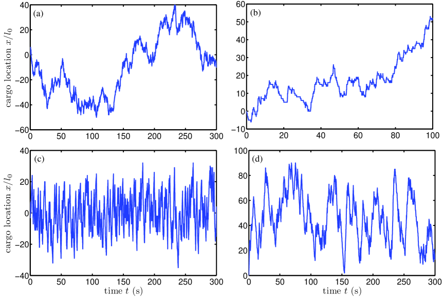
Figure 2: Trajectory samples of cargo motion by two motors under constant load (a, b), and in one fixed optical trap (c, d). For the symmetric cases (where the step rates of the plus motor are the same as the ones of the minus motor, i.e. $u=b$, $w=f$), the cargo will oscillate around its initial location (a). While for the asymmetric cases, the cargo will have nonzero mean velocity (b). If the cargo is put in one fixed optical trap and transported by two symmetric motors, it will oscillate around the trap center (c). But for the asymmetric cases, the oscillation center may be different from the trap center. For parameter values used in the simulations see Tab. I.

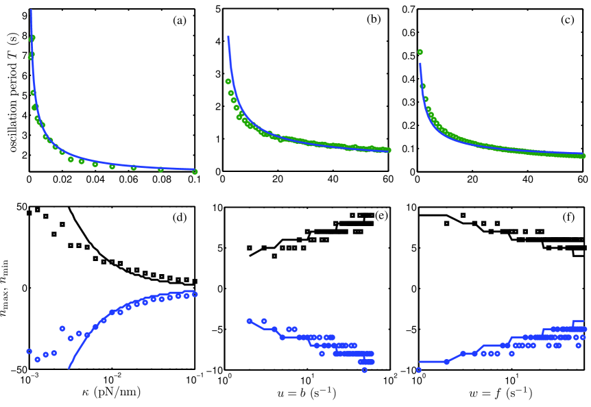
Figure 3: In fixed optical trap, the mean oscillation period $T$ of cargo decreases with trap stiffness $\kappa$, forward rates $u=b$, and backward rates $w=f$ (in fact, $\log T$ decreases almost linearly with $\log\kappa$, $\log u=\log b$, and $\log w=\log f$). The oscillation amplitude $n_{\max}-n_{\min}$ decreases with stiffness $\kappa$ and backward rates $w=f$, but increases with forward rates $u=b$. Here $n_{\max}$ and $n_{\min}$ are the $\max$ and $\min$ locations that cargo can reaches. The circles and squares are obtained by Monte Carlo simulations. In (a, b, c), the solid curves are obtained by formulation (31). The solid lines in (d) are obtained by $n_{c+},n_{c-}$ given in Eq. (11), and the solid lines in (e, f) are obtained by $n_{c+}+3,n_{c-}-3$, respectively. For parameter values see Tab. I.

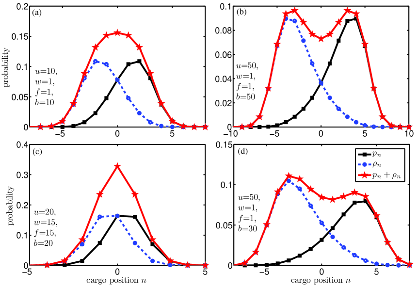
Figure 4: Samples of probability $p_{n}$ and $\rho_{n}$ for finding cargo in plus-state and minus-state. For the symmetric cases probabilities $p_{n}$ and $\rho_{n}$ are mirror symmetry to each other (a, b, c). Their sum $p_{n}+\rho_{n}$, the probability of finding cargo at location $n$, might has one maximum [at the center of optical trap, see (a, c)] or two symmetric maximum [see (b)]. (d) is one sample for the asymmetric cases. For parameter values see Tab. I.

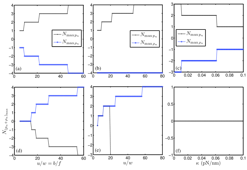
Figure 5: The location $N_{\max p_{n}},N_{\max\rho_{n}},N_{{(p_{n}+\rho_{n})}_{\max}}$ that probabilities $p_{n}$, $\rho_{n}$ and their summation $p_{n}+\rho_{n}$ reach their maximum. With the increase of rate ratio $u/w=b/f$ both $N_{\max p_{n}}$ and $N_{\max\rho_{n}}$ leave far away from the trap center (a). (b) implies that $N_{\max p_{n}}$ increases with ratio $u/w$, but $N_{\max\rho_{n}}$ is independent of it. With the increase of trap stiffness $\kappa$, both $N_{\max p_{n}}$ and $N_{\max\rho_{n}}$ come close the the trap center (c). (d, e) show that, with the increase of rate ratio $u/w=b/f$ or rate ratio $u/w$ only, the number of maximum of probability $p_{n}+\rho_{n}$ of finding cargo at location $n$ may change. But (f) implies that $N_{{(p_{n}+\rho_{n})}_{\max}}$ is independent of trap stiffness $\kappa$. For parameter values see Tab. I.

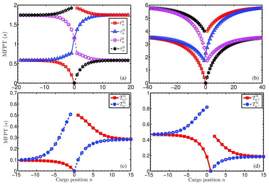
Figure 6: Samples of MFPTs $t_{n}^{0},\tau_{n}^{0}$ to plus-state $0^{+}$, MFPTs $\bar{t}_{n}^{0},\bar{\tau}_{n}^{0}$ to minus-state $0^{-}$ (a, b), and MFPT ${\cal T}_{l}^{0}$ from state $l$ to location 0 (c, d). For high trap stiffness $\kappa$, $t_{n<0}^{0}<\tau_{m<0}^{0}<\tau_{l\geq 0}^{0}<t_{k>0}^{0}$ for MPFTs to plus-state $0^{+}$, and symmetric relations hold for MFPTs to minus-state $0^{-}$, see (a). But for low trap stiffness, all MFPTs $t_{n}^{0},\tau_{n}^{0},\bar{t}_{n}^{0},\bar{\tau}_{n}^{0}$ increases with the distance between $n$ and trap center 0, see (b). Which means that, for different trap stiffness $\kappa$, the trajectories of cargo from state $n^{+}$ or $n^{-}$ to state $0^{+}$ or $0^{-}$ are different. (c, d) are MFPTs for one cargo (transported by two asymmetric motors) from state $n^{+}$ or $n^{-}$ to location 0 (plus-state $0^{+}$ or $0^{-}$) and location 1 (plus-state $1^{+}$ or $1^{-}$). The MFPT ${\cal T}_{n}^{0}$ is obtained by formulation (30). For parameter values see Tab. I.

References

- 1. Bray D (2001) Cell movements: from molecules to motility, 2nd Edn. Garland, New York.
- 2. Howard J (2001) Mechanics of Motor Proteins and the Cytoskeleton. Sinauer Associates and Sunderland, MA.
- 3. Block SM, Goldstein LSB, Schnapp BJ (1990) Bead movement by single kinesin molecules studied with optical tweezers. Nature 348: 348-352.
- 4. Vale RD (2003) The molecular motor toolbox for intracellular transport. Cell 112: 467-480.
- 5. Mallik R, Carter BC, Lex SA, King SJ, Gross SP (2004) Cytoplasmic dynein functions as a gear in response to load. Nature 427: 649-652.
- 6. Hua W, Young EC, Fleming ML, Gelles J (1997) Coupling of kinesin steps to ATP hydrolysis. Nature 388: 390-393.
- 7. Schnitzer MJ, Block SM (1997) Kinesin hydrolyses one ATP per 8-nm step. Nature 388: 386-390.
- 8. Coy DL, Wagenbach M, Howard J (1999) Kinesin takes one 8-nm step for each ATP that it hydrolyzes. J Biol Chem 274: 3667-3671.
- 9. Gennerich A, Carter AP, Reck-Peterson SL, Vale RD (2007) Force-induced bidirectional stepping of cytoplasmic dynein. Cell 131: 952-965.
- 10. Asbury CL, Fehr AN, Block SM (2003) Kinesin moves by an asymmetric hand-over-hand mechanism. Science 302: 2130-2134.
- 11. Toba S, Watanabe TM, Yamaguchi-Okimoto L, Toyoshima YY, Higuchi H (2006) Overlapping hand-over-hand mechanism of single molecular motility of cytoplasmic dynein. Proc Natl Acad Sci USA 103: 5741-5745.
- 12. Guydosh NR, Block SM (2009) Direct observation of the binding state of the kinesin head to the microtubule. Nature 461: 125-128.
- 13. Klumpp S, Lipowsky R (2005) Cooperative cargo transport by several molecular motors. Proc Natl Acad Sci USA 102: 17284-17289.
- 14. Müller MJI, Klumpp S, Lipowsky R (2008) Tug-of-war as a cooperative mechanism for bidirectional cargo transport by molecular motors. Proc Natl Acad Sci USA 105: 4609-4614.
- 15. Gennerich A, Schild D (2006) Finite-particle tracking reveals sub-microscopic size changes of mitochondria during transport in mitral cell dendrites. Phys Biol 3:45-53 3: 45-53.
- 16. Soppina V, Rai AK, Ramaiya AJ, Barak P, Mallik R (2009) Tug-of-war between dissimilar teams of microtubule motors regulates transport and fission of endosomes. Proc Natl Acad Sci USA 106: 19381-19386.
- 17. Kunwar A, Vershinin M, Xu J, Gross SP (2008) Stepping, strain gating, and an unexpected force-velocity curve for multiple-motor-based transport. Curr Biol 18: 1173-1183.
- 18. Kunwar A, Mogilner A (2010) Robust transport by multiple motors with nonlinear force-velocity relations and stochastic load sharing. Phys Biol 7: 016012.
- 19. Zhang Y (2011) Cargo transport by several motors. Phys Rev E 83: 011909.
- 20. Rogers AR, Driver JW, Constantinou PE, Jamison DK, Diehl MR (2009) Negative interference dominates collective transport of kinesin motors in the absence of load. Phys Chem Chem Phys 11: 4882.
- 21. Driver J, Rogers A, Jamison D, Das R, Kolomeisky A, et al. (2010) Coupling between motor proteins determines dynamic behaviors of motor protein assemblies. Phys Chem Chem Phys 12: 10398-10405.
- 22. Driver JW, Jamison DK, Uppulury K, Rogers AR, Kolomeisky A, et al. (2011) Productive cooperation among processive motors depends inversely on their mechanochemical efficiency. Biophys J 101: 386-395.
- 23. Jamison DK, Driver JW, Diehl MR (2011) Cooperative responses of multiple kinesins to variable and constant loads. J Biol Chem 287: 3357-3365.
- 24. Uppulury K, Efremov AK, Driver JW, Jamison DK, Diehl MR, et al. (2012) How the interplay between mechanical and non-mechanical interactions affect multiple kinesin dynamics. J Phys Chem B 116: 8846-8855.
- 25. Kunwar A, Tripathy SK, Xu J, Mattson M, Sigua R, et al. (2011) Mechanical stochastic tug-of-war models cannot explain bidirectional lipid-droplet transport. Proc Natl Acad Sci USA 108: 18960-18965.
- 26. Bouzat S, Levi V, Bruno L (2012) Transport properties of melanosomes along microtubules interpreted by a tug-of-war model with loose mechanical coupling. PLoS ONE 7: e43599.
- 27. Jülicher F, Prost J (1995) Cooperative molecular motors. Phys Rev Lett 75: 2618-2621.
- 28. Badoual M, Jülicher F, Prost J (2002) Bidirectional cooperative motion of molecular motors. Proc Natl Acad Sci USA 99: 6696-6701.
- 29. Adachi K, Oiwa K, Nishizaka T, Furuike S, Noji H, et al. (2007) Coupling of rotation and catalysis in -ATPase revealed by single-molecule imaging and manipulation. Cell 130: 309-321.
- 30. Bieling P, Telley IA, Piehler J, Surrey T (2008) Processive kinesins require loose mechanical coupling for efficient collective motility. EMBO Reports 19: 1121-1127.
- 31. Mallik R, Gross SP (2009) Intracellular transport: How do motors work together? Curr Biol 19: R416-R418.
- 32. Brouhard GJ (2010) Motor proteins: Kinesins influence each other through load. Curr Biol 20: R448-R450.
- 33. Welte MA (2010) Bidirectional transport: Matchmaking for motors. Curr Biol 20: R410-R413.
- 34. Hendricks AG, Perlson E, Ross JL, Schroeder HW, Tokito M, et al. (2010) Motor coordination via a tug-of-war mechanism drives bidirectional vesicle transport. Current Biology 20: 697-702.
- 35. Schroeder HW, Mitchell C, Shuman H, Holzbaur ELF, Goldman YE (2010) Motor number controls cargo switching at actin-microtubule intersections in vitro. Curr Biol 20: 687-696.
- 36. Leidel C, Longoria RA, Gutierrez FM, Shubeita GT (2012) Measuring molecular motor forces in vivo: Implications for tug-of-war models of bidirectional transport. Biophys J 103: 492-500.
- 37. Bell GI (1978) Models for the specific adhesion of cells to cells. Science 200: 618-627.
- 38. Fisher ME, Kolomeisky AB (2001) Simple mechanochemistry describes the dynamics of kinesin molecules. Proc Natl Acad Sci USA 98: 7748-7753.
- 39. Zhang Y (2009) A general two-cycle network model of molecular motors. Physica A 383: 3465-3474.
- 40. Zhang Y (2011) Growth and shortening of microtubules: A two-state model approach. J Biol Chem 286: 39439-39449.
- 41. Redner S (2001) A Guide to First-Passage Processes. Cambridge University Press.
- 42. Zhang Y (2011) Periodic one-dimensional hopping model with transitions between nonadjacent states. Phys Rev E 84: 031104.