A new resummation scheme in scalar field theories

Abstract

A new resummation scheme in scalar field theories is proposed by combining parquet resummation techniques and flow equations, which is characterized by a hierarchy structure of the Bethe–Salpeter (BS) equations. The new resummation scheme greatly improves on the approximations for the BS kernel. Resummation of the BS kernel in the $t$ and $u$ channels to infinite order is equivalent to truncate the effective action to infinite order. Our approximation approaches ensure that the theory can be renormalized, which is very important for numerical calculations. Two-point function can also be obtained from the four-point one through flow evolution equations resulting from the functional renormalization group. BS equations of different hierarchies and the flow evolution equation for the propagator constitute a closed self-consistent system, which can be solved completely.

1 Introduction

The Bethe-Salpeter (BS) equation plays an important role in many-body theories. It has been widely used in various research fields, e.g. the strongly correlated electron systems Bickers1989a ; Bickers1989b , hadron physics Maris1997 ; Bender1996 ; Maris2003 ; Chang2009 , particle physics, and the field theory van2002 ; Blaizot2004 ; Berges2005 ; Aarts2004 . The BS equation resums its kernel, usually called the BS kernel, to infinite order. Therefore, non-perturbative effects are included in the BS equation. However, usually in actual applications of the BS equation, it is impossible to obtain an exact kernel and we have to approximate it. For example, when the BS equation is employed to study the properties of mesons in the QCD, the usually adopted approximation is called the rainbow-ladder approximation, in which bare quark–gluon vertices are used to construct the four-quark kernel Bender1996 . However, the rainbow-ladder approximation is the simplest approximation, which loses lots of information. Lots of efforts have been made to go beyond the rainbow-ladder approximation Bender1996 ; Chang2009 .

In fact, when we employ the BS equation to describe a many-body system, the central point is whether the kernel used is good enough to obtain what are observed in experiments. If it is not enough, how can we improve it? In this work, we will discuss how to improve the approximations for the BS kernel systematically. It is found that a new resummation scheme can be used to greatly improve the approximations by employing the hierarchy structure of the BS equation.

In this work we will work under the formalism of the two-particle irreducible (2PI) effective action theory Cornwall1974 , which is also known as the $\Phi$-derivable approximations in the condensed matter physics Luttinger1960 ; Baym1962 . In the recent years, the 2PI effective action theory has attracted a lot of attention. It has been applied to calculate the entropy of the quark–gluon plasma and other thermodynamic quantities Blaizot1999 ; Berges2005a , describe the non-equilibrium dynamics with subsequent late-time thermalizationBerges2001 , compute the shear viscosity in the thermal field theory Aarts2004 , and so on. In particular, we would like to emphasize that due to many people’s contributions van2002 ; Blaizot2004 ; Berges2005 ; Reinosa2010 , it has been clear that the 2PI effective action theory can be renormalized, which is quite non-trivial for a non-perturbative approach. Therefore, in our following discussions, the renormalizability of our approximation approaches will work as a prerequisite demand. The renormalizability should not be violated at any case.

The paper is organized as follows. In Sect. 2 we discuss the hierarchy structure of the BS equation and how to improve on the approximations for the BS kernel by employing this hierarchy structure. In Sect. 3 we show how the propagator and the effective action are obtained from the four-point vertex through flow evolution equations resulting from the functional renormalization group Wetterich1993 ; Blaizot2011 . Section 4 summarizes the results and gives outlooks.

2 Hierarchy Structure of the BS Equation

We consider the following scalar field theory with a non-local regulator term

$$S_{\kappa}[\varphi]=S[\varphi]+\Delta S_{\kappa}[\varphi],$$ (1)

with

$$S[\varphi] = \frac{1}{2}\varphi_{i}iG_{0,ij}^{-1}\varphi_{j}-\frac{\lambda}{4!}\varphi^{4},$$ (2)

$$\Delta S_{\kappa}[\varphi] = -\frac{1}{2}\varphi_{i}R_{\kappa,ij}\varphi_{j},$$ (3)

where $iG_{0,ij}^{-1}=(-\partial^{2}-m^{2})\delta_{ij}$, Here summations or integrals are assumed for repeated indices. The non-local term $\Delta S_{\kappa}$ in Eq. (3) is employed to suppress quantum fluctuations whose wave lengths are larger than $1/\kappa$, where $\kappa$ has a dimension of momentum Wetterich1993 . This is achieved as follows: the non-local term in momentum space is given by

$$\Delta S_{\kappa}[\varphi]=-\frac{1}{2}\int\frac{d^{D}q}{(2\pi)^{D}}R_{\kappa}(q)\varphi(q)\varphi(-q).$$ (4)

The regulator $R_{\kappa}(q)$ is chosen to have following properties: when $q\ll\kappa$, $R_{\kappa}(q)\sim\kappa^{2}$, then the non-local term becomes a mass term with large mass $\kappa$, which suppresses quantum fluctuations with wave lengths $1/q\gg 1/\kappa$; when $q\geq\kappa$, $R_{\kappa}(q)\rightarrow 0$, so fluctuations with wave lengths $1/q\leq 1/\kappa$ are not affected. In the functional renormalization group theory, beginning from a classical action at an ultraviolet scale $\Lambda$, one can obtain the corresponding quantum action which takes into account all quantum fluctuations through the evolution of flow equations from $\kappa=\Lambda$ to 0.

From Eq. (1) we can obtain the corresponding 2PI effective action. The generating functional with one- and two-point sources is given by

$$Z_{\kappa}[J,J_{2}] = \int[d\varphi]\exp\bigg{\{}i\Big{(}S_{\kappa}[\varphi]+J_{i}\varphi_{i}+\frac{1}{2}\varphi_{i}J_{2,ij}\varphi_{j}\Big{)}\bigg{\}},$$ (5)

$$W_{\kappa}[J,J_{2}] = -i\ln Z_{\kappa}[J,J_{2}].$$ (6)

Performing the functional derivative with respect to sources, one obtains

$$\frac{\delta W_{\kappa}}{\delta J_{i}} = \langle\varphi_{i}\rangle\equiv\phi_{i},$$ (7)

$$\frac{\delta W_{\kappa}}{\delta J_{2,ij}} = \frac{1}{2}(\phi_{i}\phi_{j}+G_{ij}),$$ (8)

where $\phi$ is the expected value of the field $\varphi$ and $G$ is the full propagator. The 2PI effective action is obtained through the Legendre transformation from $W_{\kappa}[J,J_{2}]$, i.e.,

$$\Gamma_{\kappa}[\phi,G] = W_{\kappa}-J_{i}\frac{\delta W_{\kappa}}{\delta J_{i}}-J_{2,ij}\frac{\delta W_{\kappa}}{\delta J_{2,ij}}$$ (9)

$$= W_{\kappa}-J_{i}\phi_{i}-\frac{1}{2}J_{2,ij}(\phi_{i}\phi_{j}+G_{ij}).$$

Expressed in terms of $\phi$ and $G$, the 2PI effective action reads Cornwall1974

$$\Gamma_{\kappa}[\phi,G] = \frac{1}{2}\phi_{i}iG_{0\kappa,ij}^{-1}\phi_{j}+\frac{i}{2}\mathrm{Tr}\ln G^{-1}+\frac{i}{2}\mathrm{Tr}G_{0\kappa}^{-1}G+\Gamma_{\mathrm{int}}[\phi,G],$$ (10)

where we have $iG_{0\kappa}^{-1}=iG_{0}^{-1}-R_{\kappa}$ and the interacting part of the effective action is

$$\Gamma_{\mathrm{int}}[\phi,G] = \frac{1}{2}\phi_{i}i\delta G_{0,ij}^{-1}\phi_{j}+\frac{i}{2}\mathrm{Tr}\delta G_{0}^{-1}G-\frac{\lambda+\delta\lambda}{4!}\phi^{4}$$ (11)

$$-\frac{\lambda+\delta\lambda}{4}\phi^{2}G+\Gamma_{2}[\phi,G],$$

where $\Gamma_{2}$ is given by all 2PI vacuum graphs whose vertices are given by the terms cubic or quartic in $\varphi$ in the expanding expression of $S[\phi+\varphi]-S[\phi]$, and propagators are the full ones. We have employed renormalized quantities in Eq. (10) and Eq. (11). They are related to the bare quantities (with subscript B) through the following relations:

$$\delta m^{2}=Zm_{B}^{2}-m^{2}\,,~{}~{}~{}\delta\lambda=Z^{2}\lambda_{B}-\lambda\,,~{}~{}~{}\delta Z=Z-1\,.$$ (12)

$$ZG^{-1}_{0B}=G^{-1}_{0}+\delta G^{-1}_{0}\,,~{}~{}~{}\delta G^{-1}_{0}=i(\delta Z\partial^{2}+\delta m^{2})\,,~{}~{}~{}G_{B}=ZG\,.$$

In actual calculations, we must make approximations. In another words, we have to truncate the 2PI vacuum graphs included in the $\Gamma_{2}$ in Eq. (11). For example, one can expand $\Gamma_{2}$ in order of loops of skeletons, which is also known as the $\Phi$ derivable approximation; one can also expand $\Gamma_{2}$ in order of $1/N$ in the $O(N)$ model. Whatever it is, the common feature of these approximation approaches is that approximations are made to the effective action. Once the approximations are made, we can employ the approximative effective action to obtain the self-consistent equation for the two-point function. We can also obtain the BS equation for the four-point function.

In this work, we will not go the same way as those described above. We will reverse the procedure, i.e., first, we make an approximation to the BS equation, then return to the two-point function and the effective potential. Comparing our approach with the conventional one, we find that our approach has several advantages: First, our approach makes much more powerful approximations. Second, we can easily observe the hierarchy structure of the BS equations from our approach. Finally, one can employ the hierarchy structure of the BS equations to reorganize the infinite diagrams through resummation. Same as the conventional approach, our approach produces approximations which are always renormalizable. As for a non-perturbative approximation, renormalizability is a quite non-trivial demand.

In order to simplify our calculations but without lose of the generality, we consider the symmetric case in the following discussions, i.e., $\phi=0$ and 3-point vertex is also vanishing. We begin with the BS equation for the four-point vertex in the coordinate space:

$$M_{ij;kl}=\Lambda_{ij;kl}+\frac{1}{2}\Lambda_{ij;k^{\prime}l^{\prime}}G_{k^{\prime}i^{\prime}}G_{l^{\prime}j^{\prime}}M_{i^{\prime}j^{\prime};kl},$$ (13)

where the kernel is given by

$$\Lambda_{ij;kl}=4i\frac{\delta^{2}\Gamma_{\mathrm{int}}}{\delta G_{ij}\delta G_{kl}}.$$ (14)

We know that the BS equation resums diagrams in one channel to infinite order. Here we designate this channel as $s$ channel. It is also known that the renormalizability of the BS equation demands that in the kernel $\Lambda$, the two-particle reducible diagrams only can appear in the $t$ or $u$ channels. They are prohibited in the $s$ channel van2002 ; Blaizot2004 ; Berges2005 . As we have said, the $s$ channel is resummed to infinite order through the BS equation. Therefore, it is natural to remind us of the question: can we resum the two other channels to infinite order as well? In fact, inspired by the parquet resummation techniques Roulet1969 , we realize that this can be obtained by employing the BS equation once more, i.e., the kernel of the BS equation in Eq. (13) can be constructed with the solution of another BS equation. Therefore, we can express the kernel as

$$\Lambda_{ij;kl}=(\Lambda_{ij;kl}^{\mathrm{2PI}}-i\delta\lambda\delta_{ij}\delta_{ik}\delta_{il})+(M^{\prime}_{ik;jl}-\Lambda^{\prime}_{ik;jl})+(M^{\prime}_{il;jk}-\Lambda^{\prime}_{il;jk}),$$ (15)

and we have

$$M^{\prime}_{ik;jl} = \Lambda^{\prime}_{ik;jl}+\frac{1}{2}\Lambda^{\prime}_{ik;i_{1}i_{2}}G_{i_{1}j_{1}}G_{i_{2}j_{2}}M^{\prime}_{j_{1}j_{2};jl},$$ (16)

$$M^{\prime}_{il;jk} = \Lambda^{\prime}_{il;jk}+\frac{1}{2}\Lambda^{\prime}_{il;i_{1}i_{2}}G_{i_{1}j_{1}}G_{i_{2}j_{2}}M^{\prime}_{j_{1}j_{2};jk}.$$ (17)

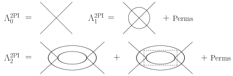
One may notice that there is another BS kernel $\Lambda^{\prime}$, but we should emphasize that $\Lambda$ and $\Lambda^{\prime}$ belong to different hierarchies and $\Lambda^{\prime}$ is lower than $\Lambda$. However, the two different BS kernels have the same symmetries, which will be discussed more carefully in the following. As one can see, there are three terms (separated by parentheses) on the right-hand side of Eq. (15). The second term corresponds to diagrams which are two-particle reducible in the $t$ channel while 2PI in the other two channels. The third term corresponds to those which are two-particle reducible in the $u$ channel while 2PI in the other two channels. The first term includes diagrams which are 2PI in all the three channels. We can see that there are no diagrams which are two-particle reducible in the $s$ channel, since this kind of diagrams are prohibited by the renormalizability of the theory. As for the diagrams included in the $\Lambda^{\mathrm{2PI}}$, which are 2PI in all the three channels, one can easily recognize that the lowest order contribution to $\Lambda^{\mathrm{2PI}}$ is just the bare vertex $\Lambda^{\mathrm{2PI}}_{0}$ as shown in Fig. 1. We also show the next two order diagrams $\Lambda^{\mathrm{2PI}}_{1}$ and $\Lambda^{\mathrm{2PI}}_{2}$ in Fig. 1, which are four and five loops, respectively. In Fig. 1 we use “Perms” to indicate all other possible permutations of external legs. One can find that there is no subdivergence in $\Lambda^{\mathrm{2PI}}_{1}$ in four dimensions, and we only need a counterterm (here denoted as $\delta\lambda_{1}$) to absorb the overall divergences. Different from the four-loop diagrams, the $\Lambda^{\mathrm{2PI}}_{2}$ has subdivergences which must be absorbed. For example, the second diagram in the second line of Fig. 1 is employed to absorb the subdivergences, and we also notice that these diagrams are also 2PI in all channels. After the subdivergences are canceled, we only need a counterterm $\delta\lambda_{2}$ to absorb the overall divergences once more. Continuing this procedure, finally we can write the first term on the right-hand side of Eq. (15) as

$$\Lambda^{\mathrm{2PI}}-i\delta\lambda=\Lambda^{\mathrm{2PI}}_{f}-i\Delta\lambda,$$ (18)

where $\Lambda^{\mathrm{2PI}}_{f}$ is not only 2PI in all channels but also finite. $\Delta\lambda$ is related with $\delta\lambda$ through the following equation:

$$\delta\lambda=\Delta\lambda+\delta\lambda_{1}+\delta\lambda_{2}+\cdots.$$ (19)

Here $\Delta\lambda$ is kept for the following use.

Figure 1: Lowest three order contributions to the diagrams which are 2PI in all the three channels.

It is easily checked that the kernel $\Lambda$ in Eq. (15) has the same symmetry as $\Lambda^{\prime}$: $\Lambda_{ij;kl}=\Lambda_{ij;lk}=\Lambda_{ji;kl}=\Lambda_{kl;ij}$. It is more convenient to discuss the renormalization in momentum space. In momentum space, we attach momenta $p$, $-p$, $-k$, $k$ with external legs whose subscripts are $i$, $j$, $k$, $l$, respectively. Then, the BS equations in Eq. (16) can be written as

$$M^{\prime}(p,-k;-p,k) = \Lambda^{\prime}(p,-k;-p,k)+\frac{1}{2}\int\frac{d^{4}q}{(2\pi)^{4}}\Lambda^{\prime}(p,-k;-q,q+k-p)$$ (20)

$$\times G(q)G(q+k-p)M^{\prime}(q,p-q-k;-p,k).$$

Here the kernel $\Lambda^{\prime}$ can be obtained by the corresponding 2PI vacuum diagrams, same as that of the conventional BS equation, which also needs to be truncated. For example, we can use 2PI vacuum diagrams up to two-loop or three-loop to obtain $\Lambda^{\prime}$, which corresponds to truncate $\Lambda^{\prime}$ to bare vertex or one-loop four-point function, respectively. Certainly, if we truncate the 2PI vacuum diagrams to higher order, we can obtain the four-point diagrams which are 2PI in all the three channels, just like the diagrams in Fig. 1. In fact, the kernel $\Lambda^{\prime}$ can also have the same structure as the $\Lambda$ in Eq. (15), which receives contributions from three different kinds of diagrams. As we have emphasized above, due to many people’s efforts and contributions, we have learned that the BS equation in Eq. (20) can be renormalized, only when the kernel $\Lambda^{\prime}$ is 2PI in the channel in which the resummation is performed through the BS equation, which is guaranteed by the 2PI property of the vacuum graphs van2002 ; Blaizot2004 ; Berges2005 . In order to make $M^{\prime}$ being finite, we need a counterterm in the kernel $\Lambda^{\prime}$. Therefore, we can express $\Lambda^{\prime}$ as a sum of a finite part and a divergent constant, i.e.,

$$\Lambda^{\prime}(p,-k;-p,k)=\Lambda^{\prime}_{f}(p,-k;-p,k)-i\Delta\lambda_{t},$$ (21)

where the subscript $t$ indicate the $t$ channel. In the same way, the BS equation in Eq. (17) in momentum space is

$$M^{\prime}(p,k;-p,-k) = \Lambda^{\prime}(p,k;-p,-k)+\frac{1}{2}\int\frac{d^{4}q}{(2\pi)^{4}}\Lambda^{\prime}(p,k;-q,q-k-p)$$ (22)

$$\times G(q)G(k+p-q)M^{\prime}(q,k+p-q;-p,-k).$$

Also, we write the kernel as

$$\Lambda^{\prime}(p,k;-p,-k)=\Lambda^{\prime}_{f}(p,k;-p,-k)-i\Delta\lambda_{u},$$ (23)

Employing $\Delta\lambda=\Delta\lambda_{s}+\Delta\lambda_{t}+\Delta\lambda_{u}$, we express Eq. (15) in momentum space as

$$\Lambda(p,-p;-k,k) = \Lambda^{\mathrm{2PI}}_{f}(p,-p;-k,k)-i\Delta\lambda_{s}$$ (24)

$$+M^{\prime}(p,-k;-p,k)-\Lambda^{\prime}_{f}(p,-k;-p,k)$$

$$+M^{\prime}(p,k;-p,-k)-\Lambda^{\prime}_{f}(p,k;-p,-k).$$

One can see that $\Lambda$ is also a sum of a finite part and a divergent constant ($\Delta\lambda_{s}$), which make the four-point vertex $M$ in the following BS equation finite:

$$M(p,-p;-k,k) = \Lambda(p,-p;-k,k)+\frac{1}{2}\int\frac{d^{4}q}{(2\pi)^{4}}\Lambda(p,-p;-q,q)$$ (25)

$$\times G^{2}(q)M(q,-q;-k,k).$$

We should emphasize that diagrams included in the kernel $\Lambda$ through resummation by Eq. (20) and Eq. (22) are 2PI in the $s$ channel, which guarantees that Eq. (25) can be renormalized.

Here we give some examples. The simplest case is that the kernel $\Lambda^{\prime}$ in Eq. (20) is just the bare vertex. Then $M^{\prime}$ is only dependent on $p-k$ and Eq. (20) can be simplified to

$$M^{\prime}(p-k) = -i(\lambda+\Delta\lambda_{t})+\frac{1}{2}[-i(\lambda+\Delta\lambda_{t})]M^{\prime}(p-k)\int\frac{d^{4}q}{(2\pi)^{4}}$$ (26)

$$\times G(q)G(q+k-p).$$

Dividing both sides of the equation with $-i(\lambda+\Delta\lambda_{t})M^{\prime}(p-k)$ and using the free propagator $G_{0}$, we obtain

$$\frac{1}{-i(\lambda+\Delta\lambda_{t})} = \frac{1}{M^{\prime}(p-k)}$$ (27)

$$-\frac{i}{2(4\pi)^{2}}\Big{(}\frac{1}{\epsilon}+\int_{0}^{1}dx\ln\frac{\bar{\mu}^{2}}{m^{2}-x(1-x)(p-k)^{2}}\Big{)},$$

where we have employed the dimensional regularization and $\bar{\mu}^{2}=4\pi\mu^{2}e^{-\gamma_{E}}$ is a mass scale. If we introduce the following renormalization condition:

$$\frac{1}{-i(\lambda+\Delta\lambda_{t})}=\frac{1}{-i\lambda}-\frac{i}{2(4\pi)^{2}}\frac{1}{\epsilon},$$ (28)

i.e.,

$$\Delta\lambda_{t}=\frac{\lambda}{1-\frac{\lambda}{2(4\pi)^{2}}\frac{1}{\epsilon}}-\lambda=\lambda\sum_{n=1}^{\infty}\Big{(}\frac{\lambda}{2(4\pi)^{2}}\frac{1}{\epsilon}\Big{)}^{n}.$$ (29)

Then we have

$$M^{\prime}(p-k)=\frac{-i\lambda}{1+\frac{\lambda}{2(4\pi)^{2}}\int_{0}^{1}dx\ln\frac{\bar{\mu}^{2}}{m^{2}-x(1-x)(p-k)^{2}}}.$$ (30)

Finally, we get the kernel $\Lambda$ as given by

$$\Lambda(p,-p;-k,k) = i\lambda+\frac{-i\lambda}{1+\frac{\lambda}{2(4\pi)^{2}}\int_{0}^{1}dx\ln\frac{\bar{\mu}^{2}}{m^{2}-x(1-x)(p-k)^{2}}}$$ (31)

$$+\frac{-i\lambda}{1+\frac{\lambda}{2(4\pi)^{2}}\int_{0}^{1}dx\ln\frac{\bar{\mu}^{2}}{m^{2}-x(1-x)(p+k)^{2}}}-i\Delta\lambda_{s},$$

where $\Lambda^{\mathrm{2PI}}$ in Eq. (24) is also truncated to bare vertex. One can easily find that the kernel $\Lambda$ has the asymptotic behavior: $\Lambda(p,-p;-k,k)-\Lambda(\tilde{p},-\tilde{p};-k,k)\sim 1/k$ at large $k$, which is the key point to renormalize the BS equation in Eq. (25).

Figure 2: Contributions to the kernel $\Lambda^{\prime}_{ik;jl}$ up to one-loop.

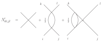
Then we consider a more complicated case and include one-loop contributions to the kernel $\Lambda^{\prime}$ in Eq. (16), which is shown in Fig. 2. From the BS equation in Eq. (16), one can rewrite $M^{\prime}$ as

$$M^{\prime}=\Lambda^{\prime}+\frac{1}{2}\Lambda^{\prime}G^{2}\Lambda^{\prime}+\frac{1}{4}\Lambda^{\prime}G^{2}\Lambda^{\prime}G^{2}\Lambda^{\prime}+....,$$ (32)

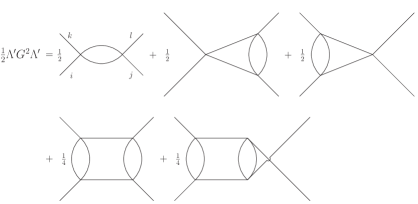
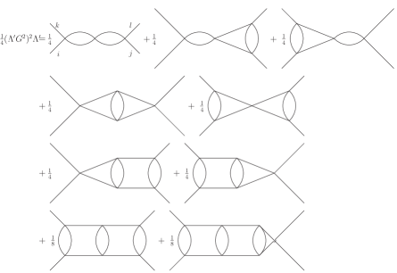
where the subscripts are not labeled explicitly. One can see that the second and third terms on the right hand side of the equation above correspond to one and two iterations. Substituting the kernel $\Lambda^{\prime}$ in Fig. 2, we get their diagram representations which are shown in Fig. 3 and Fig. 4, respectively. One can observe that all diagrams in Fig. 3 and Fig. 4 are 2PI in the $s$ channel, which confirms the renormalizability of the BS equation in Eq. (25).

Figure 3: Diagrams included in the second term on the right hand side of Eq. (32).

Figure 4: Diagrams included in the third term on the right hand side of Eq. (32).

In fact, we could generalize our approach presented above. One can use $M$ in Eq. (13) to construct the kernel of another BS equation, for example,

$$\bar{\Lambda}_{ij;kl}=(\Lambda_{ij;kl}^{\mathrm{2PI}}-i\delta\bar{\lambda}\delta_{ij}\delta_{ik}\delta_{il})+(M_{ik;jl}-\Lambda_{ik;jl})+(M_{il;jk}-\Lambda_{il;jk}),$$ (33)

which has the same structure as Eq. (15). Then this new BS equation with kernel $\bar{\Lambda}$ and the BS equations discussed above constitute a set of BS equations with three different hierarchies. One can easily check that these BS equations of different hierarchies will not result in an over-counting of diagrams. This is because Eq. (15) and Eq. (33) guarantee that the kernels are 2PI in the channel in which the summations are performed through the BS equations. This is also the reason why all the BS equations can be renormalized. This is the hierarchy structure of the BS equations.

3 Propagator and Effective Action

We have obtained the four-point vertices in the section above, and the approximations are made on the level of the four-point functions. Then the next task is to find the corresponding two-point function, i.e., the propagator which constitutes the self-consistent equations, together with the BS equations described above. In the following, we will employ the functional renormalization group to obtain the propagator.

Employing the effective action in Eq. (10), taking functional derivative with respect to the propagator and considering the stationary condition, we have

$$\frac{\delta\Gamma_{\kappa}[G]}{\delta G}\bigg{|}_{G=G_{\kappa}}=0,$$ (34)

which is in fact the gap equation as follows:

$$G_{\kappa}^{-1}=G_{0\kappa}^{-1}-\Sigma[G_{\kappa}],$$ (35)

where the self-energy $\Sigma$ is given by

$$\Sigma[G_{\kappa}]=2i\frac{\delta\Gamma_{\mathrm{int}}[G]}{\delta G}\bigg{|}_{G=G_{\kappa}}.$$ (36)

Taking derivative with respect to the flow parameter $\kappa$ on both sides of the gap equation in Eq. (35), one arrives at

$$\partial_{\kappa}G_{\kappa}^{-1}=\partial_{\kappa}G_{0\kappa}^{-1}-\partial_{\kappa}\Sigma[G_{\kappa}].$$ (37)

The first term is

$$\partial_{\kappa}G_{0\kappa}^{-1}=i\partial_{\kappa}R_{\kappa}.$$ (38)

The second term can be re-expressed as

$$\frac{\partial\Sigma[G_{\kappa}]}{\partial\kappa} = \frac{\delta\Sigma[G]}{\delta G}\bigg{|}_{G=G_{\kappa}}\frac{\partial G_{\kappa}}{\partial\kappa}$$ (39)

$$= -\frac{\delta\Sigma[G]}{\delta G}\bigg{|}_{G=G_{\kappa}}G_{\kappa}\frac{\partial G^{-1}_{\kappa}}{\partial\kappa}G_{\kappa}$$

$$= -2i\frac{\delta^{2}\Gamma_{\mathrm{int}}[G]}{\delta G\delta G}\bigg{|}_{G=G_{\kappa}}G_{\kappa}\frac{\partial G^{-1}_{\kappa}}{\partial\kappa}G_{\kappa}$$

$$= -\frac{1}{2}\Lambda[G_{\kappa}]G_{\kappa}\frac{\partial G^{-1}_{\kappa}}{\partial\kappa}G_{\kappa}.$$

Substituting Eqs. (38) (39) into Eq. (37), one finds

$$\partial_{\kappa}G_{\kappa}^{-1}=i\partial_{\kappa}R_{\kappa}+\frac{1}{2}\Lambda[G_{\kappa}]G_{\kappa}^{2}\partial_{\kappa}G^{-1}_{\kappa}.$$ (40)

Employing the BS equation in Eq. (13), we can solve $\partial_{\kappa}G_{\kappa}^{-1}$ in Eq. (40) and arrive at

$$\partial_{\kappa}G_{\kappa}^{-1}=i\partial_{\kappa}R_{\kappa}+\frac{i}{2}M[G_{\kappa}]G^{2}_{\kappa}\partial_{\kappa}R_{\kappa},$$ (41)

which is the flow equation for the propagator. Blaizot et al. derived this equation firstly and found that this flow equation is completely equivalent with the gap equation Blaizot2011 . We should emphasize that in the conventional approaches where the approximations are made in the level of the effective potential, the gap equation is easily obtained, so the flow equation for the propagator seems to be not important. However, in our case the kernel of the BS equation is resummed to infinite order through another BS equation, and it is difficult to obtain the gap equation directly. Therefore, we have to resort to the flow equation in Eq. (41). Then the BS equations (20), (22), (25), and the differential equation (41) constitute a closed system, which can be solved.

Since the propagator is obtained, the effective action can also be found. Differentiating the effective action in Eq. (10) with respect to the flow parameter $\kappa$, one finds

$$\partial_{\kappa}\Gamma_{\kappa}[G_{\kappa}] = \frac{\partial\Gamma_{\kappa}[G]}{\partial\kappa}\bigg{|}_{G=G_{\kappa}}+\frac{\partial\Gamma_{\kappa}[G]}{\partial G}\bigg{|}_{G=G_{\kappa}}\frac{\partial G_{\kappa}}{\partial\kappa}$$ (42)

$$= \frac{\partial\Gamma_{\kappa}[G]}{\partial\kappa}\bigg{|}_{G=G_{\kappa}}$$

$$= -\frac{1}{2}\mathrm{Tr}[(\partial_{\kappa}R_{\kappa})G_{\kappa}],$$

where we have used Eq. (34) in the second line. This is the flow equation for the effective action first derived in Ref. Wetterich1993 . Integrating the flow equation, one can get the effective action.

4 Summary and Outlook

In this work, we have proposed a new resummation scheme under the formalism of 2PI effective action theory. We employ the hierarchy structure of the BS equations to greatly improve on the approximations for the BS kernel. Resumming the kernel in $t$ and $u$ channels to infinite order is equivalent to truncate the effective action to infinite order. Furthermore, our approximation approaches do not violate the renormalizability of the theory, which is very important for numerical calculations. We also obtain the two-point function from the four-point one through flow evolution equations. Therefore, BS equations of different hierarchies and the flow evolution equation for the propagator constitute a closed system, which can be solved completely.

We should note that there are two hierarchies of BS equations in our approach. Therefore, comparing the conventional BS equations, we need more computer time in our calculations. But because of remarkable increases in computer power made possible by clusters, this problem is not difficult to solved.

Since we have proposed to employ the hierarchy structure of the BS equations to improve on the approximations for the BS kernel, it is very interesting to apply our approaches to detailed problems. One potential interesting problem is to compute the shear viscosity of the quark–gluon plasma or other thermal fields. As we know the shear viscosity is very sensitive to the properties of the four-point vertex, so it is expected that our approach will advance the computation of the shear viscosity. Furthermore, our approaches can also be applied to strongly correlated electron systems, for example, our approaches can be used to study the two-dimensional Hubbard model, which may shed new light on our understanding about high $T_{c}$ superconductors.