First passage times in homogeneous nucleation and self-assembly

Abstract

Motivated by nucleation and molecular aggregation in physical, chemical and biological settings, we present a thorough analysis of the general problem of stochastic self-assembly of a fixed number of identical particles in a finite volume. We derive the Backward Kolmogorov equation (BKE) for the cluster probability distribution. From the BKE we study the distribution of times it takes for a single maximal cluster to be completed, starting from any initial particle configuration. In the limits of slow and fast self-assembly, we develop analytical approaches to calculate the mean cluster formation time and to estimate the first assembly time distribution. We find, both analytically and numerically, that faster detachment can lead to a shorter mean time to first completion of a maximum-sized cluster. This unexpected effect arises from a redistribution of trajectory weights such that upon increasing the detachment rate, paths that take a shorter time to complete a cluster become more likely.

I Introduction

The self-assembly of macromolecules and particles is a fundamental processes in many physical and chemical systems. Although particle nucleation and assembly have been studied for many decades, interest in this field has recently intensified due to engineering, biotechnological and imaging advances at the nanoscale level WHITESIDES0 ; WHITESIDES1 ; GROS . Aggregating atoms and molecules can lead to the design of new materials useful for surface coatings SURFACE , electronics WIRE , drug delivery LANGER and catalysis REBEK . Examples include the self-assembly of DNA structures DNA0 ; DNA1 into polyhedral nanocapsules useful for transporting drugs BHATIA or the self-assembly of semiconducting quantum dots to be used as quantum computing bits KROUTVAR .

Other important examples of molecular self-assembly may be found in cell physiology or virology where proteins aggregate to form ion channels, viral capsids and plaques implicated in neurological diseases. One example is the rare self-assembly of fibrous protein aggregates such as $\beta-$amyloid that have long been suspected to play a role in neurodegenerative conditions such as Alzheimer’s, Parkinson’s, and Huntington’s disease SOTO . In prion diseases, individual PrP^C proteins misfold into PrP^Sc prions which subsequently self-assemble into fibrils. The aggregation of misfolded proteins in neurodegenerative diseases is a rare event, usually involving a very low concentration of prions. Fibril nucleation also appears to occur slowly; however once a critical size of about ten proteins is reached, the fibril stabilizes and the growth process accelerates NOWAK .

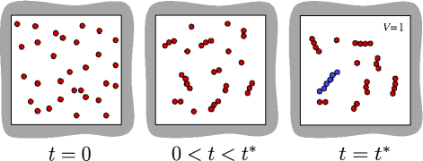
Figure 1: Homogeneous self-assembly and growth in a closed unit volume initiated with $M=30$ free monomers. At a specific intermediate time $0<t<t^{*}$ in this depicted realization, there are six free monomers, four dimers, four trimers, and one cluster of size four. For each realization of this process, there will be a specific time $t^{*}$ at which a maximum cluster of size $N=6$ in this example is first formed (blue cluster).

Viral proteins may also self-assemble to form capsid shells in the form of helices, icosahedral, dodecahedra, depending on virus type. A typical assembly process will involve several steps where dozens of dimers aggregate to form more complex subunits which later cooperatively assemble into the capsid shell. Usually, capsid formation requires hundreds of protein subunits that self-assemble over a period of seconds to hours, depending on experimental conditions ZLOTNICK ; ZLOTNICK2 .

In addition to these two examples, many other biological processes involve a fixed “maximum” cluster size – of tens or hundreds of units – at which the process is completed or beyond which the dynamics change OURJCP . At times, the assembly process may involve coagulation and fragmentation of clusters as well, such as in the case of telomere aggregation in the yeast nucleus holcman2012 . Developing a stochastic self-assembly model with a fixed “maximum” cluster size is thus important for our understanding of a large class of biological phenomena.

Theoretical models for self-assembly have typically described mean-field concentrations of clusters of all possible sizes using the well-studied mass-action, Becker-Döring equations PENROSE ; WATTIS ; SMEREKA ; OURPRE . While Master equations for the fully stochastic nucleation and growth problem have been derived, and initial analyses and simulations performed Kelly ; BHATT ; EBELING , there has been relatively less work on the stochastic self-assembly problem. We have recently shown that in finite systems, where the maximum cluster size is capped, results from mass-action equations are inaccurate and that in this case a discrete stochastic treatment is necessary DLC .

In our previous examination of equilibrium cluster size distributions derived from a discrete, stochastic model DLC , we found that a striking finite-size effect arises when the total mass is not divisible by the maximum cluster size. In particular, we identified the discreteness of the system as the major source of divergence between mean-field, mass action equations and the fully stochastic model. Moreover, discrepancies between the two approaches are most apparent in the strong binding limit where monomer detachment is slow. Before the system reaches equilibrium, or when the detachment is appreciable, the differences between the mean-field and stochastic results are qualitatively similar, with only modest quantitative disparities.

In this paper, we will be interested in the distribution of the first assembly times towards the completion of a full cluster, which can only be determined through a fully stochastic treatment. Specifically, we wish to compute the time it takes for a system of $M$ monomers to first assemble into a complete cluster of size $N$. We do not consider coagulation and fragmentation events, but, as a starting point, focus on attachment and detachment of single monomers. Statistics of the first assembly time REDNERBOOK may shed light on how frequently fast-growing protein aggregates appear. In principle, one may also estimate mean self-assembly times starting from the mean-field, mass action equations, using heuristic arguments. We will show however that these mean-field estimates yield mean first assembly times that are quite different from those obtained via exact, stochastic treatments.

In the next section, we review the Becker-Döring mass-action equations for self-assembly and motivate the formulation of approximate expressions for the first assembly time distributions. These will be shown to be poor estimates of the true distribution functions, leading us to consider the full stochastic problem in Section III. Here, we derive the Backward Kolmogorov equation associated with the self assembly process and illustrate how to formally solve it through the corresponding eigenvalue problem. In Section IV, we explore three limits of the stochastic self-assembly process and derive analytic expressions for the mean first assembly time in the strong and weak binding limits. Results from kinetic Monte-Carlo (KMC) simulations are presented in Section V and compared with our analytical estimates. Finally, we discuss the implications of our results and propose further extensions in the Summary and Conclusions.

II Mass-action model of homogeneous nucleation and self-assembly

The classic mass-action description for spontaneous, homogeneous self-assembly is the Becker-Döring model BD , where the concentrations $c_{k}(t)$ of clusters of size $k$ obey

$$\dot{c}_{1}(t) = -p_{1}c_{1}^{2}-c_{1}\sum_{j=2}^{N-1}p_{j}c_{j}+2q_{2}c_{2}+\sum_{j=3}^{N}q_{j}c_{j}$$

$$\dot{c}_{2}(t) = \displaystyle=-p_{2}c_{1}c_{2}+{\frac{p_{1}}{2}}c_{1}^{2}-q_{2}c_{2}+q_{3}c_{3}$$

$$\dot{c}_{k}(t) = -p_{k}c_{1}c_{k}+p_{k-1}c_{1}c_{k-1}-q_{k}c_{k}+q_{k+1}c_{k+1}$$

$$\dot{c}_{N}(t) = p_{N-1}c_{1}c_{N-1}-q_{N}c_{N},$$ (1)

where $p_{k}$ and $q_{k}$ are the monomer attachment and detachment rates to and from a cluster of size $k$. A typical initial condition is $c_{k}(t=0)=(M/V)\delta_{k,1}$, representing an initial state comprised only of free monomers. For simplicity we set the volume $V=1$. The above equations can be numerically integrated to find the time-dependent concentrations $c_{k}(t)$ for any set of attachment and detachment rates. We have previously shown that Eqs. 1 provide a poor approximation to the expected number of clusters when the total mass $M$ and the maximum cluster size $N$ are comparable in magnitude DLC .

Although mass action equations provide approximations to mean concentrations, they do not directly describe any statistical property of the modeled system. Nonetheless, one may be able to heuristically derive estimates of quantities such as mean first assembly times. To estimate the mean time to completion of the first maximum cluster, we must consider a truncated set of mass-action equations which treats maximum clusters as “absorbing states” so that once maximum clusters are formed, the process is stopped and the time recorded. Thus, we set $q_{N}=0$ in Eqs. 1 so that once clusters of size $N$ are formed, no detachment is allowed. This choice ensures that completed assembly events will not influence the dynamics of any of the remaining smaller clusters.

To estimate the mean first assembly time we may invoke the statistical concept of survival probabilities, and heuristically combine it with the deterministic solutions of Eq. 1. Following standard notation, we denote by $S(t)$ the probability that the system has not yet formed a maximal cluster. This quantity is also known as the “survival” probability. Its dynamics can be expressed using the probability flux $J_{N}$ out of the last not fully formed maximal cluster state, or equivalently into the maximal one, conditioned on the system still surviving so that

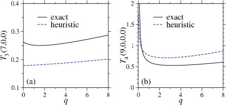
Figure 2: Mean first assembly times evaluated via the heuristic definition Eq. 7 (dashed line) and as a function of the detachment rate $q_{i}=q$, for $M=7$, $N=3$ in panel (a) and for $M=9$, $N=4$ in panel (b). Here $p_{i}=p=1$. We also show the exact results (solid line) obtained via the stochastic formulation in Eq. 12 which we derive in Section III. Qualitative and quantitative differences between the two approaches arise, which become even more evident for $N>3$, $q\to 0$, as we shall later discuss. These discrepancies underline the need for a stochastic approach.

$${{\rm d}S(t)\over{\rm d}t}=-J_{N}(t|\,\mbox{surviving up to time }\,t).$$ (2)

The flux $J_{N}(t|\,\mbox{surviving up to time }\,t)$ conditioned on survival up to time $t$ is not readily found, but a mean-field approximation can be applied by assuming $J_{N}(t|\,\mbox{surviving up to time }\,t)\approx J_{N}(t)S(t)$, where $J_{N}(t)$ is the unconstrained mean particle flux. Thus, the mean field approximation for the evolution of the survival probability becomes

$${{\rm d}S(t)\over{\rm d}t}\simeq-J_{N}(t)S(t).$$ (3)

To proceed, we may use deterministic results for $J_{N}(t)$

$$J_{N}(t)\simeq p_{N-1}c_{1}(t)c_{N-1}(t),$$ (4)

so that the survival probability can be estimated as

$$S(t)=\exp\left[-p_{N-1}\int_{0}^{t}c_{1}(t^{\prime})c_{N-1}(t^{\prime}){\rm d}t^{\prime}\right]=e^{-c_{N}(t)}.$$ (5)

Note that while Eq. 5 satisfies $S(t=0)=1$, $S(t\to\infty)\not\to 0$, due to $c_{N}(t\to\infty)$ being finite. As a consequence, the derived first assembly time will always be infinitely large, since the system has a finite survival probability even for $t\to\infty$, making the approximation invalid. Alternatively, we may approximate Eq. 2 as

$${{\rm d}S(t)\over{\rm d}t}=-J_{N}.$$ (6)

This relationship assumes that the system is always is a surviving state (not yet formed a maximum-sized cluster). However, Eq. 6 also yields unphysical results at long times. A deterministic approximation that yields physically reasonable results can be obtained by finding the time at which the concentration of clusters of size $N$ reaches unity

$$c_{N}(T_{N})\equiv 1,$$ (7)

and imposing $q_{N}=0$ in Eqs. 1. As an example, we consider the case $M=7$, $N=3$ for $p_{i}=p=1,q_{i\neq 3}=q$ (and $q_{3}=0$ as illustrated above), find $c_{N}(T_{N})$ from Eqs. 1, and plot the mean first assembly time obtained via Eq. 7 in Fig. 2(a). For completeness we also show the exact results obtained via the full stochastic treatment in Eq. 12, the derivation of which we will focus on below. What clearly arises from Fig. 2(a) is that while the mean first assembly times obtained stochastically and via the mean-field equations are of the same order of magnitude, they are also quite different and show even qualitative discrepancies. For example, the stochastic mean first assembly time is non-monotonic in $q$, while the simple mean-field estimate is an increasing function of $q$. Discrepancies between the heuristic and exact stochastic results exist also for the case $M=9$, $N=4$ shown in Fig. 2(b). Here, most notably we can point out that for $q=0$, while the exact mean first assembly time calculated according to our stochastic formulation diverges, it remains finite in the heuristic derivation. We shall later see that this trend will persist for all choices $N>3$ and that the heuristic approach does not yield accurate estimates. A stochastic treatment is thus necessary and is the subject of the remainder of this paper.

III Backward Kolmogorov Equation

To formally derive first assembly times for our nucleation and growth process it is necessary to develop a discrete, stochastic treatment. We thus define $P(n_{1},n_{2},\ldots,n_{N};t|m_{1},m_{2},\ldots,m_{N};0)$ as the probability that the system contains $n_{1}$ monomers, $n_{2}$ dimers, $n_{3}$ trimers, etc, at time $t$, given that the system started from a given initial configuration $(m_{1},m_{2},\ldots m_{N})$ at $t=0$. In this representation, the Forward Master equation corresponding to self-assembly with exponentially-distributed monomer binding and unbinding events is given by DLC

$$\dot{P}(\{n\};t|\{m\},0) = -\Lambda(\{n\})P(\{n\};t|\{m\},0)+\frac{p_{1}}{2}(n_{1}+2)(n_{1}+1)W^{+}_{1}W^{+}_{1}W^{-}_{2}P(\{n\};t|\{m\},0)$$ (8)

$$+q_{2}(n_{2}+1)W^{+}_{2}W^{-}_{1}W^{-}_{1}P(\{n\};t|\{m\},0)+\sum_{i=2}^{N-1}p_{i}(n_{1}+1)(n_{i}+1)W^{+}_{1}W^{+}_{i}W^{-}_{i+1}P(\{n\};t|\{m\},0)$$

$$+\sum_{i=3}^{N}q_{i}(n_{i}+1)W^{-}_{1}W^{-}_{i-1}W^{+}_{i}P(\{n\};t|\{m\},0),$$

where $P(\{n\},t)=0$ if any $n_{i}<0$ and

$$\Lambda(\{n\})={\frac{p_{1}}{2}}n_{1}(n_{1}-1)+\sum_{i=2}^{N-1}\!p_{i}n_{1}n_{i}+\sum_{i=2}^{N}q_{i}n_{i},$$

is the total rate out of configuration $\{n\}$. Here, $W^{\pm}_{j}$ are the unit raising/lowering operators on the number of clusters of size $i$ so that

$$W^{+}_{1}W^{+}_{i}W^{-}_{i+1}P(\{n\};t|\{m\};0)\equiv$$

$$\hskip 28.45274ptP(n_{1}+1,\ldots,n_{i}+1,n_{i+1}-1,\ldots;t|\{m\};0).$$

The Master equation can be written in the form $\dot{\bf P}={\bf A}{\bf P}$, where ${\bf P}$ is the vector of the probabilities of all possible configurations and ${\bf A}$ is the matrix of transition rates between them. The natural way of computing the distribution of first assembly times is to consider the Backward Kolmogorov equation (BKE) describing the evolution of $P(n_{1},n_{2},\ldots,n_{N};t|m_{1},m_{2},\ldots,m_{N};0)$ as a function of local changes from the initial configuration $\{m\}$. The BKE can be expressed as

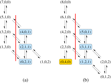
Figure 3: Allowed transitions in stochastic self-assembly starting from an all-monomer initial condition. In this simple example, the maximum cluster size $N=3$. (a) Allowed transitions for a system with $M=7$. Since we are interested in the first maximum cluster assembly time, states with $n_{3}=1$ constitute absorbing states. The process is stopped once the system crosses the vertical red line. (b) Allowable transitions when $M=8$. Note that if monomer detachment is prohibited ($q=0$), the configuration $(0,4,0)$ (yellow) is a trapped state. Since a finite number of trajectories will arrive at this trapped state and never reach a state where $n_{3}=1$, the mean first assembly time $T_{3}(8,0,0)\to\infty$ when $q=0$.

$$\dot{P}(\{n\};t|\{m\},0) = -\Lambda(\{m\})P(\{n\};t|\{m\};0)+\frac{p_{1}}{2}m_{1}(m_{1}-1)W^{+}_{2}W^{-}_{1}W^{-}_{1}P(\{n\};t|\{m\};0)$$ (9)

$$+q_{2}m_{2}W^{-}_{2}W^{+}_{1}W^{+}_{1}P(\{n\};t|\{m\};0)+\sum_{i=2}^{N-1}p_{i}m_{1}m_{i}W^{-}_{1}W^{-}_{i}W^{+}_{i+1}P(\{n\};t|\{m\};0)$$

$$+\sum_{i=3}^{N}q_{i}m_{i}W^{+}_{1}W^{+}_{i-1}W^{-}_{i}P(\{n\};t|\{m\};0),$$

where the operators $W_{i}^{\pm}$ act on the initial configuration index $m_{i}$. In the vector representation, the BKE is $\dot{\bf P}={\bf A}^{\dagger}{\bf P}$, where ${\bf A}^{\dagger}$ is the adjoint of the transition matrix ${\bf A}$ as can be verified by comparing Eqs. 8 and 9. The utility of using the BKE is that Eq. 9 can be used to determine the evolution of the survival probability, that can be naturally defined as

$$S(\{m\};t)\equiv\sum_{\{n\},n_{N}=0}P(\{n\};t|\{m\};0),$$ (10)

where we have made explicit the dependence on the initial configuration $\{m\}$. In Eq. 10 the sum is restricted to configurations where $n_{N}=0$ so as to include only “surviving” states that have not yet reached any of the ones where $n_{N}\geq 1$. $S(\{m\};t)$ thus describes the probability that no maximum cluster has yet been formed up to time $t$, given that the system started in the configuration $\{m\}$ at $t=0$. One can now similarly sum Eq. 9 over all final states with fixed $n_{N}=0$ to find that $S(\{m\};t)$ also obeys Eq. 9 with $P(\{n\};t|\{m\},0)$ replaced by $S(\{m\};t)$, along with the definition $S(m_{1},m_{2},\ldots,m_{N}\geq 1;t)=0$ and the initial condition $S(m_{1},m_{2},\ldots,m_{N}=0;0)=1$. In the vector representation where each element of ${\bf S}$ corresponds to a particular initial configuration, the general evolution equation for the survival probability is $\dot{\bf S}={\bf A}^{\dagger}{\bf S}$, where we consider only the subspace of ${\bf A}{{}^{\dagger}}$ on nonabsorbing states. Solving the matrix equation for ${\bf S}$ leads to a vector of first assembly time distributions

$${\bf G}\equiv-{\frac{\partial{\bf S}}{\partial t}},$$ (11)

where each element of ${\bf G}$ represents the first assembly time distribution starting from a different initial cluster configuration. Appendix A explicitly details the calculation procedures required to compute ${\bf S}$, ${\bf G}$, and the moments of the first assembly times. For example, using Eq. A, we find

$$T_{3}(7,0,0) = \frac{1}{105p^{2}}\frac{744p^{3}+487p^{2}q+60pq^{2}+2q^{3}}{27p^{2}+20pq+2q^{2}},$$ (12)

where we have assumed $N=3$, $M=7$, and $p_{i}=p$, $q_{i}=q$ are constants. The label $(7,0,0)$ indicates an initial condition consisting of $M=7$ monomers, no dimers, and no trimers. Corresponding expressions for the mean first assembly time arise for different initial conditions, such as e.g., $(5,1,0)$, $(3,2,0)$, or $(1,3,0)$. These exact expressions for the mean first assembly times are non-monotonic in both $q$ and $p$, indicating that there are optimal $q/p$ ratios for which the first assembly times are smallest. We will discuss the monotonicity of $T_{N}(\{m\})$ below, both in the limit of fast and slow detachment. For simplicity, we will retain the assumption of uniform $p_{i}=p$ and $q_{i}=q$ throughout the remainder of this work and henceforth rescale time in units of $p^{-1}$. With this choice, $q\gg 1$ represents fast detachment, while $q\ll 1$ represents slow detachment. $T_{3}(7,0,0)$ has already been plotted in Fig. 2(a), contrasting it against the heuristic approximation of Eq. 7. A similar matrix approach can be used for the case $M=9$, $N=4$ yielding a cumbersome but exact expression for $T_{4}(9,0,0,0)$ that is plotted in Fig. 2(b).

IV Results and Analysis

In this section we study the properties of the first assembly time in the irreversible detachment limit, when $q=0$, and in the limits of slow ($0<q\ll 1$) and fast detachment ($q\gg 1$).

IV.1 Irreversible limit ($q=0$)

First consider $N=3$ and irreversible self-assembly where $q=0$. In this case, the matrix ${\bf A}^{\dagger}$ is bidiagonal and the analysis outlined in Appendix B yields the exact expression for any starting configuration:

$$T_{3}(M-2n,n,0)=\frac{2}{(M-2n)(M-1)}\left[1+\sum_{j=1}^{[M/2]}\prod_{k=n+1}^{j}\frac{(M-2k+2)(M-2k+1)}{(M-2k)(M-1)}\right].$$ (13)

Note that when $q=0$ the mean first assembly time is finite when $M$ is odd, but is infinite if $M$ is even. This can be understood from the example $M=8$, $N=3$ illustrated in Fig. 3(b), where a “trapped” state arises. In this case, there is a finite probability that the system arrives in the state $(0,4,0)$ trapping it there forever since the assembly process is irreversible and detachment would be the only way out. Therefore, averaging over trajectories that include these “traps”, the mean assembly time will be infinite. For $q=0$, we can show that a trapped state exists for any $M$ and $N\geq 4$, yielding infinite assembly times. A trapped state arises when all free monomers have been depleted ($n_{1}=0$) before a maximum cluster has been able to assemble ($n_{N}=0$). In this case, the total mass must be distributed according to

$$M=\sum_{j=2}^{N-1}jn_{j}.$$ (14)

It is not necessarily the case that this decomposition is possible for all $M$ and $N$, but if it is, then we have a trapped state and the first assembly time is infinite. To show that the decomposition holds for $N\geq 4$ and for all $M$, we write $M=\sigma(N-1)+j$ where $\sigma$ is the integer part $[M/(N-1)]$, so that $1\leq j\leq N-2$. Now, if $j\neq 1$, then the decomposition is achieved with $n_{N-1}=\sigma$, $n_{j}=1$, and all other $n_{k}=0$ for $k\neq j,(N-1)$. We have thus constructed a possible trapped state. If instead $j=1$, then we can rewrite $M=(\sigma-1)(N-1)+(N-2)+2$ so that the decomposed state is defined by $n_{N-1}=\sigma-1$, $n_{N-2}=1$ and $n_{2}=1$, with all other values of $n_{k}=0$. This proves that for all $M,N$ there are trapped states for $q=0$. The only exception is when $N=3$, where the last decomposition does not hold, since $N-2=1$ and by definition, monomers are not allowed in trapped states. Indeed, for $N=3$, Eq. 14 gives $M=2n_{2}$ as the only trapped state, which is possible only for $M$ even. The case $M=7$ and $N=3$ is shown in Fig. 3(a).

According to our stochastic treatment, the possibility of trajectories reaching trapped states for $q=0$ exists for any value of $M,N\geq 4$, giving rise to infinite mean first assembly times. This behavior is not mirrored in the mean-field approach for $q=0$, where $c_{N}(T_{N})=1$ for finite $T_{N}$ depending on initial conditions, if $M$ is large enough as can be seen in Fig. 2(b). For $N=4$, $M=9$, indeed $T_{4}(9,0,0,0)$ can be evaluated from Eqs. 1 as $c_{4}(1.7527)=1$. In the irreversible binding limit, we may thus find instances where the exact stochastic treatment yields infinite first assembly times due to the presence of traps, while in the mean-field, mass action case, the mean first assembly time is finite. This leads us to expect that mean-field approximation to the first assembly time will be inaccurate when $q>0$, but small. Here, the trapped states (when $q=0$) retain the system for a long time.

Since infinite mean first assembly times are a consequence of the existence of trapped states one may ask what is the mean first assembly time conditioned on traps not being visited. To this end, we explicitly enumerate all paths towards the absorbed states and average the mean first assembly times only over those that avoid such traps Marcus:1968 ; Lushnikov:1978 . To be more concrete, we first consider the case $N=3$. Here, in order to reach the absorbing state where $n_{3}=1$, one or more dimers must have formed. Let us thus consider the specific case $1\leq n_{2}\leq\left[\frac{M-1}{2}\right]$. Here, the second bound arises because after $n_{2}$ dimers have formed, at least one free monomer must remain in order to attach to one of the $n_{2}$ dimers to form the first trimer. Since at every iteration both the formation of a dimer and of a trimer can occur, the probability of a path that leads to a configuration of exactly $n_{2}$ dimers is given by

$$\prod_{k=0}^{n_{2}-1}\frac{(M-2k)(M-2k-1)}{(M-2k)(M-2k-1)+2(M-2k)k},$$ (15)

The above quantity must be multiplied by the probability that after $n_{2}$ dimerizations, a trimer is formed, which occurs with probability

$$\frac{2n_{2}(M-2n_{2})}{(M-2n_{2})(M-2n_{2}-1)+2(M-2n_{2})n_{2}}.$$ (16)

Upon simplifying the product of the two probabilities in Eqs. 15 and 16, we find that the probability $W_{n_{2}}$ for a path where $n_{2}$ dimers are created before the final trimer is assembled is given by

$$W_{n_{2}}=\frac{2n_{2}}{(M-1)^{n_{2}+1}}\prod_{k=0}^{n_{2}-1}(M-2k-1).$$

Note that if $M$ is even, we must discard paths where $2n_{2}=M$, since, as described above, this case represents a trap with no monomers to allow for the creation of a trimer. According to Eq. 15, the realization $2n_{2}=M$ occurs with probability

$$W_{\frac{M}{2}}=\frac{(M-3)!!}{(M-1)^{\frac{M}{2}-1}M}.$$ (17)

Thus for $M$ even, $W_{\frac{M}{2}}$ represents the probability the system will end in a trap. We must now evaluate the time the system spends on each of the trap-free paths. Note that the exit time from a given dimer configuration $(M-2k,k,0)$ is a random variable taken from an exponential distribution with rate parameter given by the dimerization rate, $\lambda_{d,k}=(M-2k)(M-2k-1)/2$. However, the formation of a trimer is also a possible way out of the dimer configuration, with rate $\lambda_{t,k}=(M-2k)k$. The time to exit configuration $(M-2k,k,0)$ thus is itself an exponentially distributed random variable with rate $\lambda_{k}$ given by the sum of the two rates McQuarrie:1967

$$\lambda_{k}=\lambda_{d,k}+\lambda_{t,k}=\frac{(M-2k)(M-1)}{2}.$$

The typical time out of configuration $(M-2k,k,0)$ is thus given by $1/\lambda_{k}$. Upon summing over all possible values $0\leq k\leq n_{2}$, we find the typical time for the system to go through $n_{2}$ dimerizations

$$T_{n_{2}}=\sum_{k=0}^{n_{2}}\frac{1}{\lambda_{k}}=\sum_{k=0}^{n_{2}}\frac{2}{(M-2k)(M-1)}.$$

Finally, we can write the mean first assembly time as

$$T_{3}(M,0,0)=\sum_{n_{2}=1}^{\left[\frac{M-1}{2}\right]}W_{n_{2}}T_{n_{2}}.$$ (18)

It can be verified that for $M$ odd, Eq. 18 is the same as Eq. 13, since the integer part that appears in the sum in Eq. 18 is the same as its argument, thus including all paths. For $M$ even, paths with $2n_{2}=M$ are discarded, yielding a mean first assembly time averaged over trap-free configurations.

Similar calculations can be carried out for larger $N$; however, keeping track of all possible configurations before any absorbed state can be reached becomes quickly intractable. For example, when $N=4$ one would need to consider paths with a specific sequence of $n_{2,k}$ dimers formed between the creation of $k$ and $k+1$ trimers until $n_{3}$ trimers are formed. The path would be completed by the formation of a cluster of size $N=4$. We would then need to consider all possible choices for $1\leq n_{3}\leq\left[\frac{M-1}{3}\right]$ such that traps are avoided and evaluate the typical time spent on each viable path. Because of the many branching possibilities, it is clear that the enumeration becomes more and more complicated as $N$ increases.

IV.2 Slow detachment limit ($0<q\ll 1$)

Although mean assembly times are infinite in an irreversible process (except when $M$ is odd and $N=3$), they are finite when $q>0$. For general values of $M$ and $N$ and for small $q>0$, we can find the leading behavior of the mean first assembly time $T_{N}(M,0,\cdots,0)$ perturbatively by considering the trajectories from nearly trapped states into an absorbing state with at least one completed cluster.

Since the mean arrival time to an absorbing state is the sum of the probabilities of each pathway, weighted by the time taken along each of them, we expect that the dominant contribution to the mean assembly time in the small $q$ limit can be approximated by the shortest mean time to transition from a trapped state to an absorbing state. This assumption is based on the fact that the largest contribution to the mean assembly time will arise from the waiting time to exit a trap, of the order of $\sim 1/q$, since detachment is the only possible path out of the otherwise trapped state. The time to exit any other state will be of order 1 since monomer attachment is allowed. For sufficiently small detachment rates $q$, we thus expect that the dominant contribution to the mean assembly time comes from the trajectories that sample nearly trapped states and that $T_{N}(M,0,\dots,0)\sim 1/q$.

Again, first consider the tractable case $N=3$ and $M$ even, where it is clear that the sole trapped state is $(0,M/2,0)$ and the “nearest” absorbing state is $(1,M/2-2,1)$. Since the largest contribution to the first assembly time occurs along the path out of the trap and into the absorbed state, we posit

$$T_{3}(M,0,0)\simeq P^{*}(0,\frac{M}{2},0)\,T_{3}(0,\frac{M}{2},0),$$

where $P^{*}(0,M/2,0)$ is the probability of populating the trap, starting from the $(M,0,0)$ initial configuration for $q=0$. This quantity can be evaluated by considering the different weights of each path leading to the trapped state. An explicit recursion formula has been derived in our previous work DLC in Section 4 and in Eq. A.12. In the $N=3$ case however, the paths are simple, since only dimers or trimers are formed, leading to

$$P^{*}(0,\frac{M}{2},0)=\frac{(M-3)!!}{(M-1)^{\frac{M}{2}-1}M},$$ (19)

which is the same as what was derived in Eq. 17. The first assembly time $T(0,M/2,0)$ starting from state $(0,M/2,0)$ is

$${T_{3}(0,\frac{M}{2},0)=\frac{1}{\frac{M}{2}q}+T_{3}(2,\frac{M}{2}-1,0)}.$$ (20)

Here, the first term is the total exit time from the trap, given by the inverse of the detachment rate $q$ multiplied by the number of dimers. The second term is the first assembly time of the nearest and sole state accessible to the trap. This quantity can be evaluated, to leading order in $1/q$, as

$$T_{3}(2,\frac{M}{2}-1,0)\simeq\frac{1}{2(\frac{M}{2}-1)+1}\,T_{3}(0,\frac{M}{2},0),$$ (21)

where we consider that the trap will be revisited upon exiting the state $(2,M/2-1,0)$ with probability $1/(2(\frac{M}{2}-1)+1)$. In principle, Eq. 21 should also contain another term representing the possibility of reaching state $(4,M/2-2,0)$ via detachment from state $(2,M/2-1,0)$ and its contribution to the first assembly time. However, the magnitude of this term would be much smaller than $1/q$, since detachment rates are of order ${\cal O}(q)\ll{\cal O}(1/q)$. Another term that should be included in Eq. 21 is the possibility of reaching the absorbing state $(1,M/2-2,1)$. This term however, yields a zero contribution to the first assembly time. Upon combining Eqs. 20 and 21 we find that as $q\to 0$

$${T_{3}(0,\frac{M}{2},0)\simeq\frac{2(M-1)}{M(M-2)}\frac{1}{q}}.$$

Finally, $T_{3}(M,0,0)$ can be derived by multiplying the above result by Eq. 19. We can generalize this procedure to find the dominant term for the mean assembly time starting from any initial state $(M-2n,n,0)$ in the limit of small $q$, $N=3$ and for $M$ even

$$T_{3}(M,0,0)\simeq T_{3}(M-2,1,0) \simeq \frac{2(M-3)!!}{M(M-2)(M-1)^{M/2-2}}\frac{1}{q},$$ (22)

$$T_{3}(M-2n,n,0) \simeq \frac{2(M-2n-1)!!}{M(M-2)(M-1)^{M/2-n-1}}\frac{1}{q}\quad 2\leq n<M/2$$ (23)

$$T_{3}(0,M/2,0) \simeq \frac{2(M-1)}{M(M-2)}\frac{1}{q}.$$ (24)

The next correction terms do not have an obvious closed-form expression, but are independent of $q$. Note that when $q$ is small and increasing, the mean first assembly times decrease. This is also true for odd $M$. A larger $q$ leads to a more rapid dissociation, which may lead one to expect a longer assembly time. However, due to the multiple pathways to cluster completion in our problem, increasing $q$ actually allows for more mixing among them, so that at times, upon detachment, one can “return” to more favorable paths, where the first assembly time is actually shorter. This effect is clearly understood by considering the case of $q=0$ when, due to the presence of traps, the first assembly time is infinite. We have already shown that upon raising the detachment rate $q$ to a non-zero value, the first assembly time becomes finite. Here, detachment allows for visiting paths that lead to absorbed states, which would otherwise not be accessible. This same phenomenon persists for small enough $q$ and for all $M,N$ values. The expectation of assembly times increasing with $q$ is confirmed for large $q$ values, as we shall see in the next section. Taken together, these trends indicate the presence of a minimum in the mean first assembly time that occurs at an intermediate value of the detachment rate $q$.

We can generalize our estimate of the leading $1/q$ term for the first assembly time to larger values of $N$ via

$$T_{N}(M,0,\dots,0)=\sum_{\{\mu\}}P^{*}(\{\mu\})T_{N}(\{\mu\}),$$ (25)

where $\{\mu\}$ are trapped state configurations for $q=0$. The values of $P^{*}(\{\mu\})$ can be calculated as described above using the recursion formula presented in DLC . Approximate mean first assembly times $T_{N}(\{\mu\})$ from traps $\{\mu\}$ may be found by considering equations for the shortest sub-paths that link traps to each other. For instance, in the case of $M=9$, $N=4$ the only trapped states are $(0,3,1,0)$ and $(0,0,3,0)$, with associated probabilities $P^{*}(0,0,3,0)=921/5488$ and $P^{*}(0,3,1,0)=2873/24696$, respectively. The shortest path linking the two traps is $(0,3,1,0)\rightarrow(2,2,1,0)\rightarrow(1,1,2,0)\rightarrow(0,0,3,0)$, which yields, to first order, $T(0,1,3,0)=T(0,0,3,0)=1/(2q)$. Finally, from Eq. 25 we find that $T(9,0,0,0)=2005/(14112q)$ which can be verified by constructing the corresponding $D(9,4)=12$ dimensional transition matrix ${\bf A}^{\dagger}$ and solving the linear eigenvalue problem. Enumerating trajectories that intersect nearly trapped states becomes increasingly complex as $M$ and $N$ increase since more traps arise, leading to the identification of more entangled sub-paths connecting them.

IV.3 Fast detachment limit ($q\to\infty$)

We now consider the case where detachment is much faster than attachment and $q\gg M$. In this limit, we expect the full assembly of a cluster to be a rare event in the large $q$ limit, and that the mean assembly time will increase monotonically with $q$.

Dominant path approximation - Our first approximation is based on the observation that for $q\to\infty$ the dominant configurations are those with the most monomers (the higher states in each column of Fig. 3). Thus, the dominant trajectories will be the ones that most directly arrive at the absorbing state with one full cluster. For $N=3$, the overwhelmingly dominant paths are: $(M,0,0)\rightleftharpoons(M-2,1,0)\rightleftharpoons(M-3,0,1)$. The dynamics of the probabilities of the two “surviving” states with $n_{3}=0$ can be represented by a linear $2\times 2$ system that is easily solved to yield, in the $q\to\infty$ limit,

$$T_{3}(M,0,0) \simeq T_{3}(M-2,1,0)\simeq\frac{2q}{M(M-1)(M-2)},$$

The dominant path method can be generalized to any $M\geq N$ for $q\gg M$ as follows

$$\begin{array}[]{cccccccccc}(M,0,0,...,0)&\rightleftharpoons&(M-2,1,0...,0)&\rightleftharpoons&\cdots&\rightleftharpoons(M-r,0...,1,..,0)&\rightleftharpoons&\cdots&\rightleftharpoons&(M-N,0,...0,1).\end{array}$$ (26)

Here, the corresponding transition matrix ${\bf R}^{\dagger}$ is tridiagonal and of dimension $(N-1)$ with elements $r^{\dagger}_{1,1}=-r^{\dagger}_{1,2}=-M(M-1)/2$ and $r^{\dagger}_{k,k-1}=q,r^{\dagger}_{k,k}=-q-(M-k),r^{\dagger}_{k,k+1}=(M-k)$ for $2\leq k\leq(N-1)$. The inverse of ${\textbf{R}}^{\dagger}$ can be computed by a three-term recurrence formula USMANI . After some algebraic manipulation, we can write the first assembly time along the path in Eq. 26 for any $M\geq N$ and for $q\geq M$ as

$$T_{N}(M,0,\dots,0)=\frac{2q^{N-2}}{\prod_{i=0}^{N-1}(M-i)} \Bigg{[} \sum_{k=0}^{N-2}\prod_{\ell=1}^{k}(M-(N-\ell))q^{-k}$$

$$+ \frac{M(M-1)}{2}\sum_{j=2}^{N-2}\prod_{\ell=2}^{j-1}(M-\ell)\sum_{k=0}^{N-j-1}\prod_{l=1}^{k}(M-(N-\ell))q^{1-j-k}\Bigg{]}.$$

Our notation is such that products with the lower index larger than the upper one are set to unity. In Eq. IV.3, the largest term in the $q\to\infty$ limit is given by

$$T_{N}(M,0,\dots,0)\simeq\frac{2q^{N-2}}{\prod_{i=0}^{N-1}(M-i)}.$$

The additional assumption $M\gg N$ on the other hand, leads to the approximation $M-i\simeq M$ so that Eq. IV.3 becomes

$$T_{N}(M,0,\dots,0)\simeq\frac{q^{N-1}}{M^{N}}\Bigg{[}\sum_{k=2}^{N-1}\frac{(k-1)M^{k}}{q^{k}}+\frac{2}{q}\sum_{k=0}^{N-2}\frac{M^{k}}{q^{k}}\Bigg{]}.$$ (28)

Results for other choices of initial configurations $\{m\}$ can be obtained by following the same reasoning illustrated here. We expect $T_{N}(\{m\})$ not to be too different from $T_{N}(M,0,\dots,0)$ in the strong detachment $q\to\infty$ case when any initial clusters will rapidly disassemble, leading the system towards the free monomer configuration. The distribution of first assembly times can also be obtained within the dominant path approximation, as outlined in Appendix C.

We expect these results to hold for large $q\geq M$, small values of $N$ and moderate values of $M$ so that the most likely trajectories follow the dominant path. However, due the possibility of many branching paths in configuration space, modest changes in $\{M,N,q\}$ may allow sampling of secondary paths that yield different estimates of the first assembly time. Indeed, as both $M$ and $N$ become larger, the creation of several intermediate clusters may be more favorable than progressively adding monomers to the largest one. In the next subsection we thus introduce a “hybrid” approach, where the possibility of having multiple intermediate aggregates is included by assuming that the first $r$ clusters are distributed according to the Becker-Döring equilibrium distribution and the remaining $N-r$ follow a monomer-to-largest cluster path towards complete assembly.

Hybrid approximation - We now consider a different approach to the fast detachment $q\to\infty$ limit by using a “pre-equilibrium” or “quasi steady-state” approximation powers06 that partially neglects correlations between some of the cluster numbers by separating time scales between fast and slow varying quantities. We will use the pre-equilibrium approximation on the stochastic formulation of Eq. 8; however, to illustrate the method, we will first apply it to Eqs. 1, with $q_{N}=0$

The equilibrium values $c^{\rm eq}_{i}$ arising from Eqs. 1 where $p_{i}=1$ are given by

$$c_{i}^{\rm eq}=\frac{(c_{1}^{\rm eq})^{i}}{2q^{i-1}},$$

for $2\leq i\leq N$, whereas $c_{1}^{\rm eq}$ can be obtained using the mass conservation constraint

$$c_{1}^{\rm eq}+\frac{1}{2}\sum_{i=2}^{n}\frac{i}{q^{i-1}}(c_{1}^{\rm eq})^{i}=c_{1}(0)=M.$$

We can now define the fluxes $J_{i}^{\pm}(t)$

$$J_{i}^{+}(t) \equiv c_{1}(t)c_{i-1}(t) \simeq\frac{(c_{1}^{\rm eq})^{i}}{2q^{i-2}},$$

$$J_{i}^{-}(t) \equiv qc_{i+1}(t) \simeq\frac{(c_{1}^{\rm eq})^{i}}{2q^{i-2}},$$

for $1\leq i\leq N-1$. Note that as $q\to\infty$ all fluxes decrease and that since $q$ is large, $J_{i}^{\pm}(t)\gg J_{i+1}^{\pm}(t)$. This implies that smaller clusters experience faster dynamics and motivates the quasi-steady state approximation. We may thus consider the first $N-1$ reactions to be at equilibrium so that Eqs. 1 can be rewritten as a function of the mass $x(t)$ contained in all clusters except the largest one:

$$x(t)=\sum_{i=1}^{N-1}ic_{i}(t).$$ (29)

Eqs. 1 now become

$$\dot{x}(t) = -N\dot{c}_{N}(t)=-\frac{N}{2q^{N-2}}c_{1}(x)^{N},$$ (30)

where $c_{1}(x(t))$ satisfies

$$c_{1}+\frac{1}{2}\sum_{i=2}^{N-1}\frac{i}{q^{i-1}}(c_{1})^{i}=x.$$ (31)

Upon solving Eq. 31, we can obtain $c_{1}(x)$, which can then be inserted in Eq. 30 to determine $c_{N}(t)$ and $x(t)$. Upon using the crude approximation $c_{1}(x)\approx x$ in Eq. 30 we can solve for $x(t)$ and find the time at which $c_{N}=1$, or equivalently $x=M-Nc_{N}=M-N$

$$T_{N}(M,0,\ldots,0)=\frac{q^{N-2}}{N}\left[\frac{N-1}{(M-N)^{N-1}}-\frac{N-1}{M^{N-1}}\right].$$

A more accurate result can be found by allowing the sum in Eq. 31 to go to infinity so that

$$c_{1}(x)=\frac{-q+\sqrt{4qx+q^{2}}}{2}.$$

Using this expression in Eq. 30, the mean mass in the fast clusters $x(t)$ can be explicitly computed. Note that we could as well have assumed that only the first $1\leq r<N-1$ clusters equilibrate among themselves, and solved a reduced system of $N-r+1$ equations. We do not pursue this explicitly here, and move directly to the stochastic version of pre-equilibration.

A separation of time scales can also be performed in stochastic systems, where the basic assumptions for pre-equilibration are the same as for the deterministic case. In particular, we require the “fast” subsystem to be ergodic and to possess a unique equilibrium distribution. The dynamics of the “slow” subsystem is then obtained by averaging the fast variables over their equilibrium distribution; the basic assumption is that while slow variables evolve, the fast ones equilibrate instantaneously to their average values Kang . As we shall see, due to the equilibrium hypothesis, summing Eq. 8 over the variables that constitute the fast subsystem, will lead to the vanishing of all terms that do not modify the slow variable, and all remaining terms will involve averages of the fast variable Haseltine2005 .

Just as in the deterministic case, we allow the first $N-1$ cluster sizes to equilibrate amongst each other and write the probability distribution function using a mean-field approach

$$P(\{n\};t|\{m\},0)=P_{\rm eq}(\{n^{\prime}\}|n_{N})P(n_{N};t|\{m\},0).$$ (32)

For fixed $n_{N}$, $P_{\rm eq}(\{n^{\prime}\}|n_{N})$ represents the equilibrium distribution function for the first, fast $\{n^{\prime}\}=\{n_{1},\dots,n_{N-1}\}$ cluster sizes and

$$P(n_{N};t|\{m\},0)=\sum_{\{n^{\prime}\}}P(\{n^{\prime}\},n_{N};t|\{m\},0)\,$$ (33)

is the probability distribution for the last, slow cluster size $n_{N}$. The sum in Eq. 33 is to be performed over all values of $\{n^{\prime}\}$ such that mass conservation $\sum_{i}^{N-1}in_{i}=M-Nn_{N}$ is obeyed. Note that while $P_{\rm eq}(\{n^{\prime}\}|n_{N})$ does not depend on the initial conditions of the $\{n^{\prime}\}$ clusters, it does depend on $n_{N}$. Upon inserting the ansatz in Eq. 32 in Eq. 8 and performing the summation over all configurations $\{n^{\prime}\}$ with fixed $n_{N}$, we find

$$\dot{P}(n_{N};t|\{m\},0) = -\big{(}\langle n_{1}n_{N-1}|n_{N}\rangle_{\rm eq}+qn_{N}\big{)}P(n_{N};t|\{m\},0)$$

$$+\langle n_{1}n_{N-1}|n_{N}-1\rangle_{\rm eq}P(n_{N}-1;t|\{m\},0)+q(n_{N}+1)P(n_{N}+1;t|\{m\},0).$$

In Eq. LABEL:MASTER_reduce, we have used the notation

$$\langle n_{1}n_{N-1}|n_{N}\rangle_{\rm eq}=\sum_{\{n^{\prime}\}}n_{1}n_{N-1}P_{\rm eq}(\{n^{\prime}\}|n_{N})$$ (35)

representing the equilibrium second moment $\langle n_{1}n_{N-1}|n_{N}\rangle_{\rm eq}$, which is an average over all fast variables with the added constraint that they have total mass $M-Nn_{N}$. Eq. LABEL:MASTER_reduce implies that $n_{N}$ follows a Markovian birth and death process with birth rate $\langle n_{1}n_{N-1}|n_{N}\rangle_{\rm eq}$ and a death rate $qn_{N}$. Starting at $n_{N}=0$ at time $t=0$, the first birth event coincides with the first assembly time so that the survival probability can be written as

$$S_{N-1}(t)=\exp\Big{[}-\int_{0}^{t}\langle n_{1}n_{N-1}|n_{N}=0\rangle_{\rm eq}{\rm d}t\Big{]}\equiv e^{-\lambda t},$$ (36)

where the “$N-1$” indicates that all clusters of size $N-1$ and smaller have been pre-equilibrated. Having defined $\lambda=\langle n_{1}n_{N-1}|n_{N}=0\rangle_{\rm eq}$ in Eq. 36, the first assembly time distribution is exponential

$$G_{N-1}(\{m\};t)=\lambda e^{-\lambda t},$$ (37)

and the mean first assembly time is given by $T_{N}(M,\cdots,0)=1/\lambda$. The remaining difficulty lays in determining the quantity $\langle n_{1}n_{N-1}|n_{N}\rangle_{\rm eq}$. We may resort to a very crude approximation, by simply using the Becker-Döring results

$$\langle n_{1}n_{N-1}|n_{N}\rangle_{\rm eq} \simeq c_{1}^{\rm eq}c_{N-1}^{\rm eq}$$

$$\simeq \frac{1}{2q^{N-2}}(c_{1}^{\rm eq})^{N}.$$

Eq. IV.3 can now be used to estimate $\lambda$ and all other related quantities. Our work so far implies that the first assembly time is exponentially distributed according to Eq. 37. However, upon comparing with results from Monte-Carlo simulations in the next section, we will show that the $N-1$ pre-equilibration and is often not a good approximation. As outlined in Appendix D, a less drastic approximation can be implemented by allowing only the first $r$ species ($1\leq r<N$) to pre-equilibrate. This more restricted pre-equilibration approximation can occasionally provide better fits to simulation as we will see in the next section.

V Comparison with Simulations

In this section we present results derived from simulations of the stochastic process associated to the probability distribution process for various values of $\{M,N,q\}$. Specifically, we use an exact stochastic simulation algorithm (kinetic Monte-Carlo, KMC) to calculate first assembly times BKL75 ; GILLESPIE77 . For each set of $\{M,N,q\}$ we sample at least $10^{4}$ trajectories and follow the time evolution of the cluster populations until $n_{N}=1$, when the simulation is stopped and the first assembly time recorded. We compare and contrast our numerical results with the analytical approximations evaluated in the previous sections.

We begin with the simple case of $M=7$ and $N=3$ in Fig. 4(a) where we plot the mean first assembly time $T_{3}(7,0,0)$ as a function of $q$ obtained via our exact results Eq. 12 and by runs of 10⁵ KMC trajectories. Numerical and exact analytical results are in very good agreement, in contrast to the discrepancies between the fully stochastic and mean field treatments observed in Fig. 2. For comparison, we also plot in Fig. 4(b) the mean first assembly time $T_{3}(8,0,0)$ for $M=8$ and $N=3$, where the presence of the trapped state $(0,4,0)$ leads to a diverging first assembly time for $q=0$ and to the asymptotic behavior $T_{3}(8,0,0)\sim 1/q$ for $q\to 0$, as predicted. Note that as discussed above $T_{3}(7,0,0)$ is finite for $q=0$ due to the lack of trapped states for $N=3$ and $M$ odd. We do not plot the first assembly time distributions as their features are similar to ones we will later discuss.

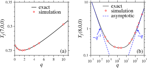
Figure 4: Mean first assembly times for $M=7$ and $N=3$ in panel (a) and $M=8$ and $N=3$ in panel (b). Exact results derived in Eq. 12 are plotted as black solid lines, while red circles are obtained by averaging over $10^{5}$ KMC trajectories. The dashed blue line shows the $q\to 0$ approximation in Eq. 22 and the $q\to\infty$ approximation in Eq. IV.3.

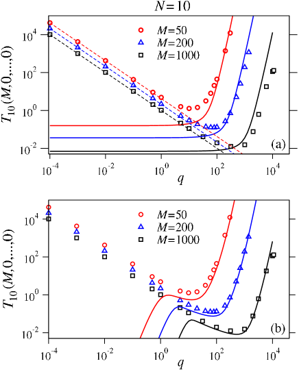
Figure 5: Comparison of theory with simulations for $N=10$, and several values of $M$. Symbols are derived from $10^{4}$ KMC simulations for $M=50,200,1000$. In panel (a) the dashed lines are obtained by plotting the curve $T_{10}(M,0,\dots,0)=A/q$ where $A$ is given by imposing passage through the first point to the left in the graph. Note that all other points align to the same curve. Solid lines are derived from Eq. IV.3 in the dominant path approximation. In panel (b) results from the hybrid approximation with $r=2$ in Eq. D are superimposed on the same data. Note the much better fit in the hybrid approximation as $q\to\infty$, especially as $M$ becomes larger.

We generalize this analysis by plotting numerical estimates of $T_{10}(M,0,\cdots,0)$ as a function of $q$ for various values of $M$ in Fig. 5(a). As expected, for small $q$, the mean first assembly time scales as $1/q$ for all values of $M$. Similarly, for all values of $M$, the first assembly time presents a minimum, due to the previously-described increased weighting of faster pathways upon increasing $q$ for small enough values of $q$. For larger values of $q$ we expect the most relevant pathways towards assembly to be the ones constructed along the linear chain described in (26). Indeed, we find that in accordance with Eq. 28$,T_{N}(M,0,\cdots,0)\simeq 2q^{N-2}/M^{N}$ as $q\geq M$. Small and large $q$ estimates using the dominant path approximation are shown in Fig. 5(a).

As discussed earlier, the dominant path approximation becomes less accurate as $M$ increases, since the linear chain pathway neglects other possible routes towards complete assembly, that become relevant as $M$ increases. In Fig. 5(b) thus we plot the same data points, using the hybrid approximation discussed above for large $q$, with $r=2$. Note a much closer fit with the simulation data, especially as $M$ increases.

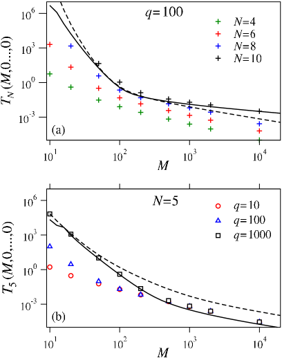
Figure 6: First assembly times $T_{N}(M,0,\dots,0)$ as a function of $M$ for $q=100$ and several values of $N$ in panel (a), and for $N=5$ and several values of $q$ in panel (b). The black dashed lines represent the dominant path approximation for large $q$ in Eq. IV.3, while the solid black line represents the hybrid approximation in Eq. D for $r=2$. We chose to plot only representative cases, not to clutter the graphics, but similar trends persist in panel (a) for $N=4,6,8$ and in panel (b) for $q=10,100$. Note that the dominant path approximation ceases to be accurate for very large values of $M$ and that the hybrid approximation provides a better fit as $q\to\infty$.

In Fig. 6(a) we plot $T_{N}(M,0,\cdots,0)$ as a function of $M$ for $q$ fixed and various $N$, while in Fig. 6(b) $T_{N}(M,0,\dots,0)$ is plotted as a function of $M$ for $N$ fixed and various $q$. Both Figs. 6(a) and 6(b) show that the results derived in Eq. IV.3 for large $q$ using the dominant path approximation are accurate provided $M$ is not too large compared to $N$. As shown by the black solid lines, in this case $T_{N}(M,0,\cdots,0)\simeq 2q^{N-2}/M^{N}$. For larger values of $M$, the dominant path approximation becomes inaccurate: numerical results indicate that $T_{N}(M,0,\cdots,0)\simeq 1/M^{\nu}$ with $\nu\sim 1$ as $q\to\infty$. In this regime, the hybrid approximation with $r=3$ yields a better fit, as shown by the solid lines in Figs. 6(a) and  6(b).

Finally, in Figs. 7–9 we plot the distribution function $G(\{M,0,\cdots,0\},t)$ of the first assembly times for several representative choices of $\{M,N,q\}$. As illustrated in the figure captions, analytical estimates were calculated either by inverse Laplace transforming Eq. 46 after having numerically found its poles, or via the hybrid approximation in Eq. D with specific values of $r$. From Fig. 7 note upon increasing $q$, $G(\{M,0,\dots,0\},t)$ gradually shifts from having a log-normal shape towards an exponential distribution characterized by the decay rate evaluated in Eq. 48. Some combinations of $M$ and $N$, such as $M=200$ and $N=8$ in Fig. 8 yield a bimodal distribution for small $q$. This can be explained by noting that while fast routes towards nucleation may exist, other pathways lead the system to the previously described trapped states where $n_{1}=n_{N}=0$. Exit from these traps is unlikely for small $q$, yielding larger first assembly times. The emergence of a bimodal distribution should be more apparent for larger values of $N$ when there is a longer pathway towards assembly and more potential traps. Indeed, although not shown in Fig. 7 for $M=50$ and $N=4$, a few trajectories populate the region $t\sim 1/q$, indicating passage through at least one of the nine possible trapped states. However, the weights of these possible paths are very small (only about 10 or so out of $10^{4}$ runs incurred into a trapped state), so we do not include them in Fig. 7 which is truncated at $t\ll 1/q$, when $q\to 0$. This occurs also for $M=8$ and $N=3$, where a minor spread due to the $(0,4,0)$ trap and centered around $t\sim 1/q$ arises in the distribution tail, and which is absent from the trap-free case of $M=7$ and $N=3$.

Note that although few paths may populate the region $t\sim 1/q$ their contribution to the mean first assembly time may be significant. In Fig. 8 we also include analytical estimates of the first assembly times: the dashed red curves are derived from the dominant path approximation in Eq. 46 and the solid blue ones from the hybrid approximation in Eq. D using $r=3$. As noted above, for very large $q$, the dominant path approximation fails and the hybrid approximation provides a closer fit to our numerical results.

In Fig. 9, we plot the first assembly time distribution for fixed $q=100$ and $N=8$ and varying $M$. As expected, for $q\geq M$, $G(\{M,0,\cdots,0\},t)$ is well approximated by the exponential distribution in Eq. 49. As $M$ increases the distribution acquires a log-normal shape. In this case, we find the hybrid approximation to fail regardless of $r$. Indeed, our numerical results show that there is no specific criterion to ensure that the hybrid approximation will yield even qualitatively valid estimates for the first assembly distributions as $M\to\infty$. Empirically, we find that while mean first assembly times predictions are quite accurate within the hybrid approximation, the first assembly distribution estimates are more likely to be accurate when the are exponentially distributed.

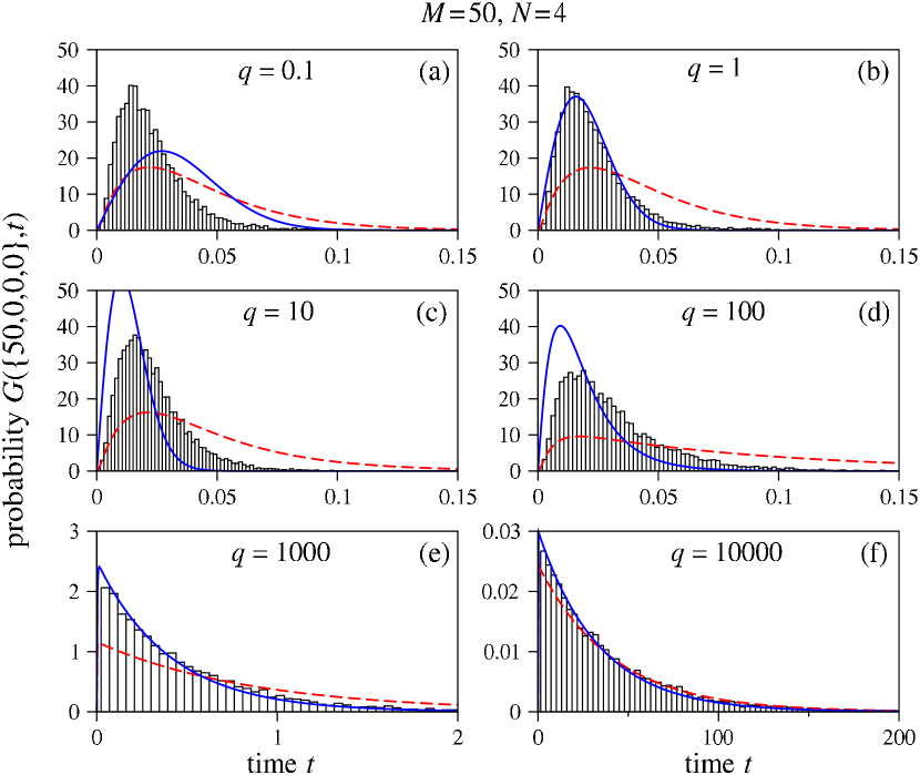
Figure 7: Probability distributions for the first assembly time for $N=4$ and $M=50$ and for various values of $q$. The black bars are obtained as a normalized histogram of $10^{4}$ KMC simulations. The dashed red and solid blue lines are the probability density functions estimated via the dominant path approximation in Eq. 46 and via the hybrid approximation with $r=3$ in Eq. D, respectively. The detachment rate $q$ increases as indicated in each subplot. Note that initially the distribution has a log-normal shape and later turns into an exponential. As predicted, the analytical estimate given by Eq. 46 becomes accurate for $q\geq M$. Also note the change in scale and the broadening of the distribution as $q$ increases.

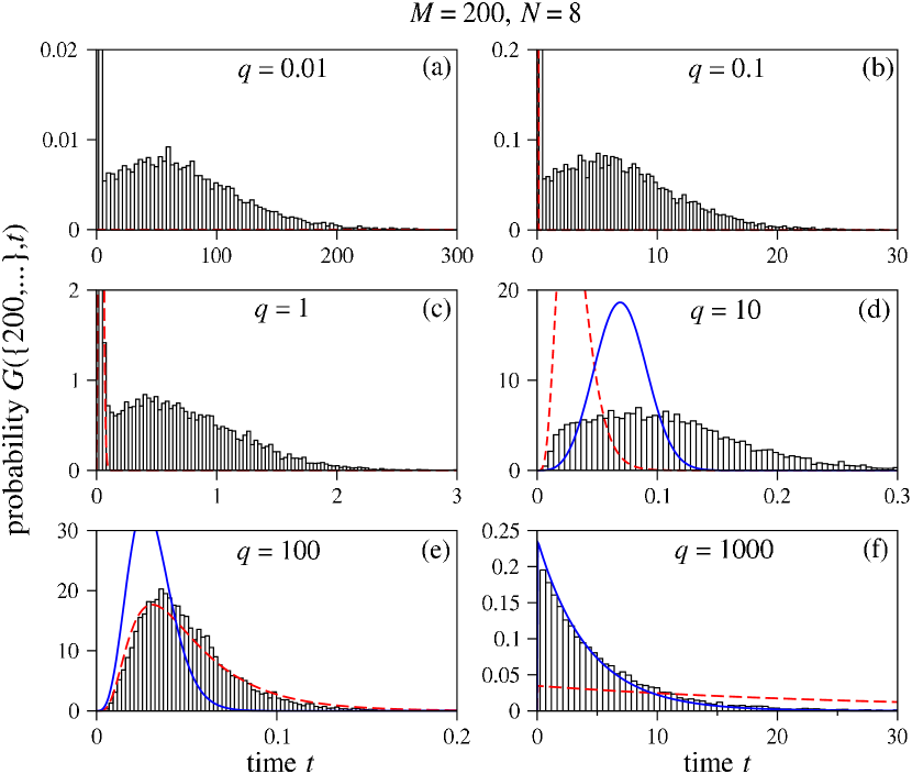
Figure 8: First assembly time distributions for $N=8$ and $M=200$ for various values of $q$. The black bars are obtained as a normalized histogram of $10^{4}$ KMC simulations. The dashed red and solid blue lines are the probability density functions estimated via the dominant path approximation in Eq. 46 and via the hybrid approximation with $r=3$ in Eq. D respectively. The detachment rate $q$ increases as indicated in each subplot. Note that the distribution evolves from a bi-stable curve to, later acquiring a log-normal shape, before turning to an exponential. As above, as $q\to\infty$ the hybrid approximation yields a closer fit to the numerical data.

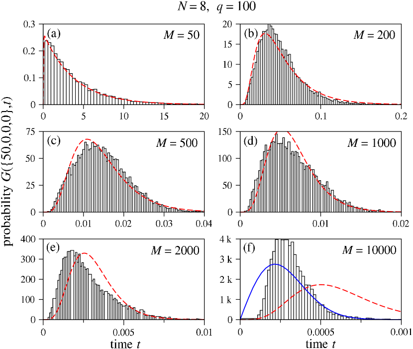
Figure 9: First assembly time distributions for $N=8$ and $q=100$ for various values of $M$. The black bars are obtained as a normalized histogram of $10^{5}$ KMC simulations. The dashed red and solid blue lines are the probability density functions estimated via the dominant path approximation in Eq.  (46) and via the hybrid approximation with $r=3$ in Eq. D respectively. Total mass $M$ increases as indicated in each subplot. Note that the distribution evolves from an exponential with decay rate given by Eq. 48, valid for $q\geq M$, towards a more log-normal shape. In this case, for very large $M$ both dominant path and hybrid approximation fail.

VI Summary and Conclusions

We have studied the problem of determining the first assembly time of a cluster of a pre-determined size $N$ to form from an initial pool of $M$ independent monomers characterized by uniform attachment and detachment rates $p=1$ and $q$, respectively. We have shown that while heuristic approaches using the traditional Becker-Döring equations can be developed, these fail to capture relevant qualitative features, such as divergences and non-monotonic behavior. A full stochastic approach, based on the Backward Kolmogorov equation, was investigated.

We developed our stochastic model and were able to find exact results for the first assembly time in systems where $M,N$ are small enough for analytical treatments to be feasible. For general $M,N$ we were able to estimate general trends and behaviors for both large and small $q$. In particular, we find that in the absence of detachment, when $q=0$, trapped states arise from which the system is never able to escape, leading to infinitely large first assembly times. Furthermore, we showed that these traps arise for all values of $N>3$, regardless of $M$. The possibility of a trap, and of diverging first assembly times is not captured by the heuristic approach, and is confirmed by our KMC simulations. We are also able to show that for small $q$, the divergence in the first assembly time scales as $1/q$. The latter result may appear counter-intuitive, since larger detachment rates should intuitively hinder the assembly process, leading to the expectation that larger $q$ implies larger first assembly times. While this is true in the $q\to\infty$ limit, in the case of $q\to 0$ an opposite trend arises: the increased accessibility of potential paths in configuration space that lead to more rapid first assembly times. As $q$ increases, these new paths become increasingly populated, yielding an overall decrease in the first assembly time. Finally, for larger values of $q$ we identify the most likely path to be traveled in phase space towards the first assembly of an $N$-cluster and derive estimates for the associated first assembly time and probability distribution functions. For $q\gg 1$, we also considered a “hybrid” approach where the first few clusters were allowed to equilibrate, while the larger ones were still evolving stochastically. In certain cases we were able to find better agreement with numerical data, while for other combinations of $\{M,N,q\}$ the hybrid approach fails. The collection of analytic approaches for the limits $q=0$, $0<q\ll 1$, and $q\gg 1$ are outlined in Sections IV A, B, and C, respectively.

All of our analytical results were confirmed by our KMC simulations, from which we obtained first assembly times and related probability distribution functions. For certain choices of $\{M,N,q\}$ the presence of traps could be indirectly inferred by the emergence of bimodal distributions with very large first assembly times (on paths where traps were encountered) and very short ones (on others that were able to avoid them). These bimodal distributions may be smeared out for other choices of $\{M,N,q\}$.

A number of additional stochastic properties of our self-assembly problem can be calculated. For example, one can derive analogous results for attachment and detachment rates $p_{k}$ and $q_{k}$ that depend on cluster size $k$. In particular, if we assume that binding and unbinding of monomers depends on the available surface area, and that clusters are of spherical shape, we can use the forms $p_{k},q_{k}\sim k^{2/3}$. Similarly, one could assume that stoichiometric limitations could exist so that attachment of monomers becomes progressively slower as completion of the $N$-mer is approached so that $p_{k}\sim(N-k)$ and $q_{k}\sim k$. These extensions as well as the treatment of heterogeneous nucleation and first “breakup” times will be considered in future work.

VII Acknowledgements

R.Y. was supported by ANR grant 08-JCJC-0135-01. This work was also supported by the National Science Foundation through grants DMS-1021850 (MRD) and DMS-1021818 (TC). MRD was also supported by an ARO MURI grant (W1911NF-11-10332), while TC was also supported by ARO grant 58386MA.

Appendix A Calculation of Survival probability and moments

To obtain expressions for moments of the first assembly time, it is useful to Laplace transform Eq. 11 so that

$$\tilde{\bf G}={\bf 1}-s\tilde{\bf S}.$$

Here, $\tilde{\bf G}$ and $\tilde{\bf S}$ are Laplace transforms of ${\bf G}$ and ${\bf S}$, respectively. The vector ${\bf 1}$ is the survival probability of any initial, nonabsorbing state, and consists of 1’s in a column of length given by the dimension of ${\bf A}^{\dagger}$ on the subspace of nonabsorbing states. Using this representation we may evaluate the mean assembly time for forming the first cluster of size $N$ starting from the initial configuration $\{m\}$

$$T_{N}(\{m\}) \equiv -\int_{0}^{\infty}t\frac{\partial S(\{m\};t)}{\partial t}{\rm d}t$$

$$= \int_{0}^{\infty}S(\{m\};t){\rm d}t=\tilde{S}(\{m\};s=0),$$

Similarly, the variance ${\rm V}_{N}(\{m\})$ of the first assembly time can be expressed as

$${\rm V}_{N}(\{m\}) \equiv -\int_{0}^{\infty}t^{2}\frac{\partial S(\{m\};t)}{\partial t}{\rm d}t-T_{N}^{2}(\{m\})$$ (40)

$$= 2\int_{0}^{\infty}tS(\{m\};t){\rm d}t-T_{N}^{2}(\{m\})$$

$$= -2\,\frac{\partial\tilde{S}(\{m\},s)}{\partial s}\bigg{|}_{s=0}-\tilde{S}^{2}(\{m\};0).$$

Upon Laplace-transforming $\dot{\bf S}={\bf A}^{\dagger}{\bf S}$ and applying the initial condition $S(\{m\};t=0)={\bf 1}$, we find

$$\tilde{\bf S} = [s{\bf I}-{\bf A}^{\dagger}]^{-1}{\bf 1},$$ (41)

so that

$$\tilde{\bf G}={\bf 1}-s[s{\bf I}-{\bf A}^{\dagger}]^{-1}{\bf 1}.$$

The first assembly time starting from a specific configuration $\{m\}$ is thus

$$T_{N}(\{m\}) = \tilde{S}(\{m\};0)=-\left[({\bf A}^{\dagger})^{-1}{\bf 1}\right]_{\{m\}},$$ (42)

where the subscript $\{m\}$ refers to the vector element corresponding to the $\{m\}^{\rm th}$ initial configuration. Similar expressions can be found for the variance and other moments.

In order to invert the matrix ${\bf A}^{\dagger}$ on the subspace of non-absorbing states we first note that its dimension $D(M,N)$ rapidly increases with $M$. In particular, we find that the number of distinguishable configurations with no maximal cluster obeys the recursion

$$D(M,N+1)=\sum_{j=0}^{\left[M/N\right]}D(M-jN,N),$$ (43)

where $\left[M/N\right]$ denotes the integer part of $M/N$. For example, in Eq. 43, $D(M,2)=1$, and the only “surviving” configuration not to have reached at least one cluster of size $k=2$ is $(M,0)$. The next term is $D(M,3)=1+\left[M/2\right]$ which, for $M\to\infty$ yields $D(M,3)\simeq M/2$. Similarly, $D(M,4)$ can be written as

$$D(M,4)=\sum_{j=0}^{\left[M/3\right]}D(M-3j,3)\simeq\left[\frac{M}{3}\right]\left[\frac{M}{2}\right]\simeq\frac{M^{2}}{6},$$

where the last two approximations are valid for large $M$. By induction, we find

$$D(M,N)\simeq\frac{M^{N-2}}{(N-1)!}.$$

From these estimates, it is clear that the complexity of the eigenvalue problem in Eq. 42 increases dramatically for large $M$. This enumeration of states and the associated matrix method for computing first assembly times is analogous to the study of first passage times on a network benichou . However, rather than considering statistical properties of a scale free network, we are concerned with a probability flux across a specific realization of a state space network.

We begin by studying the case of $N=3$ for general $M$ where instructive explicit solutions can be derived for the mean assembly times. In this case, the eigenvalue problem for the vector of survival probabilities ${\bf S}\equiv(S(M,0,0;t),S(M-2,1,0;t),S(M-4,2,0;t),\ldots)$ can be written using a tridiagonal transition matrix ${\bf A}^{\dagger}$ whose elements $a^{\dagger}_{i,j}=a_{j,i}$ take the form

$$a^{\dagger}_{k,k-1} = (k-1)q_{2},\quad 2\leq k\leq 1+\left[\frac{M}{2}\right]$$

$$a^{\dagger}_{k,k} = -\frac{(M-2k+2)(M-2k+1)}{2}p_{1}-(k-1)q_{2}-$$

$$(k-1)(M-2k+2)p_{2},\quad$$

$$\hskip 76.82234pt1\leq k\leq 1+\left[\frac{M}{2}\right]$$

$$a^{\dagger}_{k,k+1} = \frac{(M-2k+2)(M-2k+1)}{2}p_{1},\quad$$

$$\hskip 76.82234pt2\leq k\leq 1+\left[\frac{M}{2}\right]$$

where the first (second) index denotes the column (row) of the matrix. Using the above form for ${\bf A}^{\dagger}$, we can now symbolically or numerically solve for the Laplace-transformed survival probability ${\tilde{S}}(\{m\};s)$ and the mean self-assembly time ${\tilde{S}}(\{m\};s=0)$.

Appendix B Calculation procedure for irreversible limit $q=0$

When $q=0$, the matrix ${\bf A}^{\dagger}$ now becomes bi-diagonal and a two-term recursion can be used to solve for the survival probability $\tilde{S}(M-2n,n,0;s)$ as follows. If the entries of the bidiagonal matrix ${\bf A}^{\dagger}$ are denoted $a^{\dagger}_{ij}$, then the elements $b_{i,j}$ of the inverse matrix ${\bf B}=\left[s{\bf I}-{\bf A}^{\dagger}\right]^{-1}$ are given by

$$b_{i,i} = \frac{1}{s-a^{\dagger}_{i,i}},$$

$$b_{i,j} = 0\quad\mbox{if $i>j$},$$ (44)

$$b_{i,j} = \displaystyle{\frac{\prod_{k=i}^{j-1}a^{\dagger}_{k,k+1}}{\prod_{k=i}^{j}(s-a^{\dagger}_{k,k})}}\quad\mbox{if $i<j$},.$$

The Laplace-transformed survival probability, according to Eq. 41 is the sum of entries of each row of $\left[s{\bf I}-{\bf A}^{\dagger}\right]^{-1}$

$$\tilde{S}(M-2n,n,0;s)=\frac{1}{s-a^{\dagger}_{i,i}}+\!\!\sum_{j=i+1}^{[M/2]+1}\!\!\displaystyle{\frac{\prod_{k=i}^{j-1}a^{\dagger}_{k,k+1}}{\prod_{k=i}^{j}(s-a^{\dagger}_{k,k})}},$$ (45)

where $i=n+1$ is the $(n+1)^{\rm st}$ row of $\left[s{\bf I}-{\bf A}^{\dagger}\right]^{-1}$. Upon performing the inverse Laplace transform of Eq. 45 we can write the survival probability $S(M-2n,n,0;t)$ as a sum of exponentials and derive the full first assembly time distribution $-\partial S(M-2n,n,0;t)/\partial t$. Similarly, the mean first assembly time, according to Eq. 42, is $T_{3}(M-2n,n,0)=\tilde{S}(M-2n,n,0;s=0)$. In particular, from Eq. B we find

$$\frac{a^{\dagger}_{k,k+1}}{a^{\dagger}_{k+1,k+1}}=-\frac{(M-2k+2)(M-2k+1)}{(M-2k)(M-1)},$$

which, when inserted into Eq. 45 with $s=0$ leads to Eq. 13.

Appendix C Calculation procedure for fast detachment $q\gg 1$

An estimate for the first assembly time distribution can be obtained within the dominant path assumption (Eq. 26). By using the symmetry properties of the associated matrix ${\textbf{R}}^{\dagger}$ we can find the Laplace transform of the first assembly time distribution $G(\{M,0,\dots,0\};s)$ CHEMLA in the $q\geq M$ limit

$$\tilde{G}(\{M,0,\dots,0\};s)=\frac{\frac{1}{2}\prod_{i=0}^{N-1}(M-i)}{d_{N-1}(s)},$$ (46)

where $d_{N-1}(s)$ is a unitary polynomial of degree $N-1$, given by the following recurrence

$$d_{1} = s+\frac{M(M-1)}{2},$$

$$d_{2} = (s+(M-2)+q)d_{1}-q\frac{M(M-1)}{2},$$ (47)

$$d_{i} = (s+(M-i)+q)d_{i-1}-q(M-(i-1))d_{i-2},$$

$$\mbox{ for $i>2$}.$$

Thus, $d_{N-1}(s)=s^{N-1}+...+\beta s^{2}+\alpha s+\frac{1}{2}\prod_{i=0}^{N-1}(M-i)$. Note that the first assembly time is given by

$$T_{N}(M,0,\dots,0)=\lim_{s\to 0}\frac{1-\tilde{G}(\{M,0,\dots,0\};s)}{s}.$$

By comparing Eq. 46 with Eq. IV.3 we note that the term $\alpha$ that appears in the above expansion for $d_{N-1}(s)$, corresponds to the quantity in the square brackets in Eq. IV.3 so that

$$T_{N}(M,0,\dots,0)=\frac{2\alpha}{\prod_{i=0}^{N-1}(M-i)}.$$

and $\alpha=q^{N-2}+$ h.o.t. One can also calculate the variance of the first assembly time distribution to obtain

$${\rm V}_{N}(M,0,\dots,0) = \frac{\alpha^{2}}{\prod_{i=0}^{N-1}(M-i)^{2}}$$

$$-\frac{2\beta}{\prod_{i=0}^{N-1}(M-i)},$$

and similarly all other moments of the distribution. Finally, we can also estimate the first assembly time distribution $G(\{M,0\dots,0\},t)$ by considering the inverse Laplace transform of Eq. 46, specifically by evaluating the dominant poles associated to $d_{N-1}(s)$. In the large $q$ limit, $d_{N-1}(s)$ as evaluated via the recursion relations Eqs. 47 can be approximated as

$$d_{N-1}(s)\simeq q^{N-2}s+\frac{1}{2}\prod_{i=0}^{N-1}(M-i),$$

yielding the slowest decaying root $\lambda_{N}$

$$\lambda_{N}=-\frac{1}{2q^{N-2}}\prod_{i=0}^{N-1}(M-i).$$ (48)

The above estimate allows us to write $G(\{M,0,\dots,0\};t)$ in the large $q$ limit as an exponential distribution with rate parameter $\lambda_{N}$

$$G(\{M,0,\dots,0\};t)\simeq\frac{e^{\lambda_{N}t}}{2q^{N-2}}\prod_{i=0}^{N-1}(M-i)$$ (49)

Appendix D Hybrid approximation for $q\gg 1$ and $r<N-1$

A more general hybrid approximation can be implemented by assuming that only cluster of size $r$ and smaller pre-equilibrate. We integrate Eq. 8 over all configurations but with $n_{r+1},...n_{N}$ fixed and obtain a reaction network for the remaining $N-r$ clusters:

$$\large\begin{array}[]{ccccccccc}n_{r}&\xrightleftharpoons[qn_{r+1}]{\langle n_{1}n_{r}|\{n_{r+1}\}\rangle_{\rm eq}}&n_{r+1}&\xrightleftharpoons[qn_{r+2}]{\langle n_{1}|\{n_{r+1}\}\rangle_{\rm eq}n_{r+1}}&n_{r+2}&\cdots&\xrightarrow[]{\langle n_{1}|\{n_{r+1}\}\rangle_{\rm eq}n_{N-1}}&n_{N},\end{array}$$ (50)

where $\{n_{r+1}\}=\{n_{r+1},\cdots,n_{N}\}$ so that $\langle n_{1}n_{r}|\{n_{r+1}\}\rangle_{\rm eq}$ and $\langle n_{1}|\{n_{r+1}\}\rangle_{\rm eq}$ depend on the slowly varying mass, $M-\sum_{r+1}^{N}in_{i}$, just as above for the choice $r=N-1$.

In the reaction chain (50) the last cluster size $n_{N}$ is treated as an absorbing state since we are only interested in the first assembly time, when $n_{N}=1$. The question still remains of properly evaluating $\langle n_{1}n_{N-1}|\{n_{r+1}\}\rangle_{\rm eq}$ and $\langle n_{1}|\{n_{r+1}\}\rangle_{\rm eq}$. For $q\to\infty$ it is reasonable to argue that that most of the mass is distributed among the fast clusters $n_{1},...n_{r}$. Indeed, if we now assume that all the mass is contained in the fast cluster sizes, $\langle n_{1}|\{n_{r+1}\}\rangle_{\rm eq}$ and $\langle n_{1}n_{r}|\{n_{r+1}\}\rangle_{\rm eq}$ may be obtained via a distribution of $r$ clusters with total mass $M-\sum_{i=r+1}^{N}in_{i}\simeq M$. The rates in (50) become independent of $n_{i}$, for $i>r$. We can also drop the slow cluster size condition on the averaged quantities, and simply write $\langle n_{1}\rangle_{M}$ and $\langle n_{1}n_{r}\rangle_{M}$.

The cluster network in (50) is a so-called linear Jackson queueing network Kingman1969 . Entry of particles in queue $n_{r+1}$ occurs at rate $\langle n_{1}n_{r}\rangle_{M}$, each of them moving independently according to the forward $\langle n_{1}\rangle_{M}$ and backward $q$ transition rates. Starting with no particles in the queue at $t=0$, the time-dependent probability distribution for this queueing network is well known Kingman1969 . In particular, the number of particles in the last queue follows a Poisson distribution with mean

$$\mu(t)=\langle n_{1}n_{r}\rangle_{M}\int_{0}^{t}{\cal P}_{N-r}(s){\rm d}s$$

where ${\cal P}_{i}(t)$ is the probability that a single particle is in the $i^{th}$ queue at time $t$ after its entry in the system. Because the last queue is absorbing, and from the definition of the first assembly time, the survival probability of our clustering process can be identified with the probability of having no particles in the last queue so that

$$S(t) = \mbox{Prob}\{n_{N}=0\}$$

$$= \exp\Big{[}-\langle n_{1}n_{r}\rangle_{M}\int_{0}^{t}{\cal P}_{N-r}(s)\,{\rm d}s\Big{]}.$$

Finally, note the probability ${\cal P}_{i}(t)$, for $1\leq i\leq N-r$ satisfies the Master equation $\dot{\cal P}_{i}=A_{ij}{\cal P}_{j}$ with $P_{i}(0)=\delta_{1i}$ and

$$A_{ij}=\left(\begin{array}[]{cccccc}-q-\langle n_{1}\rangle_{M}&\hskip 11.38092ptq&&&&0\\ \langle n_{1}\rangle_{M}&\hskip 11.38092pt-q-\langle n_{1}\rangle_{M}&\hskip 11.38092ptq&&&0\\ &\hskip 11.38092pt\ddots&\hskip 11.38092pt\ddots&\ddots&&0\\ &&&\langle n_{1}\rangle_{M}&-q-\langle n_{1}\rangle_{M}&0\\ &&&0&\langle n_{1}\rangle_{M}&0\end{array}\right),$$

The first assembly time and the variance can now be derived according to standard formulae in Eq. A and Eq. 40.

As before, this technique requires an estimation of the first and second moments $\langle n_{1}\rangle_{M}$ and $\langle n_{1}n_{r}\rangle_{M}$ from the equilibrium distribution for clusters up to size $r$ with total mass $M$. A first crude way of approximating these asymptotic moments is to use the mean-field results

$$\langle n_{1}\rangle_{M} \simeq c_{1}^{\rm eq},\quad\langle n_{1}n_{N-1}\rangle_{M}\simeq c_{1}^{\rm eq}c_{N-1}^{\rm eq}.$$

We can also derive moment equations for $\langle n_{1}\rangle_{M}$ and $\langle n_{1}n_{r}\rangle_{M}$ directly from Eq. 8. Here, due to non-linear couplings between cluster sizes, the lower order moments will necessarily be described in terms of higher order ones. For instance, to determine the first and second moments we are interested in, we would need an expression for the third moment. To close moment equations, one usually assumes that the probability distribution for all cluster sizes obeys a certain form – either Gaussian, log-normal or negative binomial which are among the most standard. The third moment may then be written as a function of the first two, thus closing the system. The closed equations of the first two moments become non-linear and a numerical solver is typically used to solve them GILLESPIE . The case $r=2$ has been extensively analyzed in CAO . In this paper we follow the same approach, using a Gaussian distribution to approximate higher moments, thus deriving a closed system of $r$ equations for $\langle n_{i}\rangle_{M}$ and $r(r+1)/2$ equations for $\langle n_{i}n_{j}\rangle_{M}$, where $1\leq i,j\leq r$.

Finally, note that the hybrid approach described above is based on the assumption that all mass is initially contained within the first $r$ clusters and are distributed according to the Becker-Döring equilibrium distribution. We expect this approach to be valid for moderate and large values of $M$ and $N$, with $q\geq M$ in order for the production of small clusters to be faster than the production of larger ones. How to choose the optimal cutoff value $r$ is a delicate issue and depends on the specific parameters $\{M,N,q\}$, although in general we find that all values of $2\leq r\leq N-2$ give qualitatively similar results.

References

- (1) G. M. Whitesides and M. Boncheva, Beyond molecules: self-assembly of mesoscopic and macroscopic components, Proc. Natl. Acad. Sci. USA 99 4769-4774 (2002).
- (2) G. M. Whitesides and B. Grzybowski, Self-assembly at all scales, Science 295 2418-2421 (2002).
- (3) R. Groß and M. Dorigo, Self-assembly at the macroscopic scale, Proc. IEEE 96 1490-1508 (2008).
- (4) W. K. Cho, S. Park, S. Jon, and I. S. Choi, Water-repellent coating: formation of polymeric self-assembled monolayers on nanostructured surfaces, Nanotechnology 18 395602 (2007).
- (5) H. Yan, S. H. Park, G. Finkelstein, J. H. Reif, and T. H. Labean DNA-templated self-assembly of protein arrays and highly conductive nanowires, Science 301 1882-1884 (2003).
- (6) O. C. Farokhzad and R. Langer, Impact of nanotechnology on drug delivery, ACS Nano 3 16-20 (2009).
- (7) J. Kang, J, Santamaria, G. Hilmersson and J. Rebek Jr., Self-assembled molecular capsule catalyzes a Diels-Alder reaction, J. Am. Chem. Soc. 120 7389-7390 (1998).
- (8) J. Chen and N. C. Seeman, Synthesis from DNA of a molecule with the connectivity of a cube, Nature 350 631-633 (1991).
- (9) C. A. Mirkin, R. L. Letsinger, R. C. Mucic, and J. J. Storhoff, A DNA-based method for rationally assembling nanoparticles into macroscopic materials, Nature 382 607-609 (1996).
- (10) D. Bhatia, S. Mehtab, R. Krishnan, S. S. Indi, A. Basu and Y. Krishnan, Icosahedral DNA nanocapsules by modular assembly, Angew. Chemie 48 4134-4137 (2009).
- (11) M. Kroutvar, Y. Ducommun, D. Heiss, M. Bichler, D. Schuh, G. Abstreiter and J. J. Finley, Optqically programmable electron spin memory using semiconductor quantum dots, Nature 432 81-84 (2004).
- (12) C. Soto, Unfolding the role of protein misfolding in neurodegenerative diseases, Nature Rev. Neurosci. 4 49-60 (2003).
- (13) J. Masela, V.A.A. Jansena, M. A. Nowak, Quantifying the kinetic parameters of prion replication, Biophys. Chem 77 139-152 (1999).
- (14) A. Zlotnick, To build a virus capsid: an equilibrium model of the self assembly of polyhedral protein complexes, J. Mol. Biol. 241 59-67 (1994).
- (15) A. Zlotnick, Theoretical aspects of virus capsid assembly, J. Mol. Recogn. 18 479-490 (2005).
- (16) M. Gibbons, T. Chou, M. R. D’Orsogna, Diffusion-dependent mechanisms of receptor engagement and viral entry, J. Phys. Chem. B 114 15403-15412 (2010).
- (17) N. Hozé and D. Holcman, Coagulation-fragmentation for a finite number of particles and application to telomere clustering in the yeast nucleus, Phys. Lett. A 376 845-849 (2012).
- (18) O. Penrose, The Becker-Döring equations at large times and their connection with the LSW theory of coarsening, J. Stat. Phys. 89 305-320 (1997).
- (19) J. A. D. Wattis and J. R. King, Asymptotic solutions of the Becker-Döring equations, J. Phys. A: Math. Gen. 31 7169-7189 (1998).
- (20) P. Smereka, Long time behavior of a modified Becker-Döring system, J. Stat. Phys. 132 519-533 (2008).
- (21) T. Chou and M. R. D’Orsogna, Coarsening and accelerated equilibration in mass-conserving heterogeneous nucleation, Phys. Rev. E 84 011608 (2011).
- (22) F. Schweitzer, L. Schimansky-Geier, W. Ebeling, and H. Ulbricht, A stochastic approach to nucleation in finite systems: theory and computer simulations, Physica A 150 261-279 (1988).
- (23) F.P. Kelly, Reversibility and stochastic networks, (Cambridge Mathematical Library, 1979)
- (24) J. S. Bhatt and I. J. Ford, Kinetics of heterogeneous nucleation for low mean cluster populations, J. Chem. Phys. 118 3166-3176 (2003).
- (25) M. R. D’Orsogna, G. Lakatos, and T. Chou, Stochastic self-assembly of incommensurate clusters, J. Chem. Phys. 136 084110 (2012).
- (26) S. Redner, A guide to first passage processes, (Cambridge University Press, 2001).
- (27) R. Becker, W. Döring, Kinetische behandlung der keimbildung in übersättigten dämpfen, Annalen der Physik 24 719-752 (1935).
- (28) S. Condamin, O. Bénichou, V. Tejedor, R. Voituriez and J. Klafter, First-passage times in complex scale-invariant media, Nature 450 77-80 (2007).
- (29) A. H. Marcus, Stochastic Coalescence, Technometrics, 10 133-143 (1968).
- (30) A. A. Lushnikov, Coagulation in Finite Systems, J. Coll Inter. Scie. 65 276-285 (1978).
- (31) D. A. McQuarrie, Stochastic approach to chemical kinetics, J. Appl. Probability, 4 413-478 (1967).
- (32) R.A. Usmani, Inversion of a tridiagonal Jacobi matrix, Lin. Alg. Appl. 212 413-414 (1994).
- (33) Y. R. Chemla, J. R. Moffitt, and C. Bustamante, Exact solutions for kinetic models of macromolecular dynamics, J. Phys. Chem. B 112 6025-6044 (2008).
- (34) E. T. Powers and D. L. Powers, The kinetics of nucleated polymerizations at high concentrations: amyloid fibril formation near and above the supercritical concentration, Biophys. J. 91 122-132 (2006).
- (35) H.W. Kang and T. G. Kurtz, Separation of time-scales and model reduction for stochastic reaction networks, To appear in Annals of Applied Prob, (2012).
- (36) E. L. Haseltine and J. B. Rawlings, On the origins of approximations for stochastic chemical kinetics, J. Chem. Phys. 122 164115-164116 (2005).
- (37) J. F. C. Kingman, Markov Population Processes, J. Appl. Prob. 6 1-18 (1969).
- (38) Y. Cao, D.T. Gillespie and L.R. Petzold, The slow-scale stochastic simulation algorithm, J. Chem. Phys 122 1-18 (2005).
- (39) C. S. Gillespie, Moment-closure approximations for mass-action models, IET Syst. Biol. 3 52-58 (2009).
- (40) A. B. Bortz, M. H. Kalos, and J. L. Lebowitz, A new algorithm for Monte Carlo simulation of Ising spin systems, J. Comp. Phys. 17 10-18 (1975).
- (41) D.T. Gillespie, Exact Stochastic Simulation of Coupled Chemical Reactions, J. Phys. Chem. 81 2340-2361 (1977).
- (42) S. Ilie, W. H. Enright and K. R. Jackson, Numerical solution of stochastic models of biochemical kinetics, Can. Appl. Math. Quart. 17 523-554 (2009).
- (43) M. Pineda-krch, Implementing the stochastic simulation algorithm in R J.Stat. Soft. 25 1-18 (2008).