Kepler Studies of Low-Mass Eclipsing Binaries I. Parameters of the Long-Period Binary KIC 6131659^†

Abstract

KIC 6131659 is a long-period (17.5 days) eclipsing binary discovered by the Kepler mission. We analyzed six quarters of Kepler data along with supporting ground-based photometric and spectroscopic data to obtain accurate values for the mass and radius of both stars, namely $M_{1}=0.922\pm 0.007\,M_{\odot}$, $R_{1}=0.8800\pm 0.0028\,R_{\odot}$, and $M_{2}=0.685\pm 0.005\,M_{\odot}$, $R_{2}=0.6395\pm 0.0061\,R_{\odot}$. There is a well-known issue with low mass ($M\lesssim 0.8\,M_{\odot}$) stars (in cases where the mass and radius measurement uncertainties are smaller than two or three percent) where the measured radii are almost always 5 to 15 percent larger than expected from evolutionary models, i.e. the measured radii are all above the model isochrones in a mass-radius plane. In contrast, the two stars in KIC 6131659 were found to sit on the same theoretical isochrone in the mass-radius plane. Until recently, all of the well-studied eclipsing binaries with low-mass stars had periods less than about three days. The stars in such systems may have been inflated by high levels of stellar activity induced by tidal effects in these close binaries. KIC 6131659 shows essentially no evidence of enhanced stellar activity, and our measurements support the hypothesis that the unusual mass-radius relationship observed in most low-mass stars is influenced by strong magnetic activity created by the rapid rotation of the stars in tidally-locked, short-period systems. Finally, using short cadence data, we show that KIC 6131657 has one of the smallest measured non-zero eccentricities of a binary with two main sequence stars, where $e\cos\omega=(4.57\pm 0.02)\times 10^{-5}$.

1 Introduction

Double-lined eclipsing binaries (DLEBs) are the best known way of accurately measuring the masses and radii of stars (see Torres, Andersen, & Giménez 2010, for a recent review). Although recent discoveries in interferometry, asteroseismology, and other methods provide promising new ways for measuring stellar radii, these techniques still lack the precision of DLEBs in almost all cases.

Comparisons of DLEBs with predicted mass-radii relations from stellar models have been made for a variety of stellar masses. However, until recently, only a few systems in the low-mass regime were well characterized, mostly because of difficulties in observing these systems. Those low-mass systems that had been observed showed radii consistently about 10-15% higher than predictions from stellar and evolutionary models (see, for example Torres & Ribas 2002; Ribas 2006; López-Morales 2007; Ribas et al. 2008). The most common explanation for this discrepancy is that tidal interactions in short period systems causes higher than normal rotational speeds, which in turn increase the level of stellar activity (Pizzolato et al. 2003; López-Morales 2007).

If the above explanation for the bloated radii of the low-mass stars is true, one would expect to find low mass binaries that have large separations (and periods) to have a normal mass-radius relationship. Unfortunately, it can be difficult to identify and observe long period DLEBs with ground based instrumentation. K and M dwarfs can be faint, and large numbers of them need to be monitored for long periods of time to find eclipses. Not that long ago, only two low mass DLEBs were known, CM Dra (Lacy 1977; Metcalfe et al. 1996), and YY Gem (Bopp 1974; Leung & Schneider 1978). Recently, in the past decade or so, various ground based surveys have detected several more (see e.g. Ribas 2006; Çakirli, İbanoǧlu, & Dervişoǧlu 2011; Bhatti et al. 2010; Becker et al. 2011; Kraus et al. 2011). However, nearly all of these have had short periods of less than about three days. Notable exceptions include T-Lyr1-17236 with a pair of M-stars in an 8.4 day orbit (Devor et al. 2008), Kepler-16 with a pair of low-mass stars in a 41 day orbit (Doyle et al. 2011), and LSPM J1112+7626 with a pair of M-stars that are also in a 41 day orbit (Irwin et al. 2011).

NASA’s Kepler mission offers an exciting opportunity in this field of study. Kepler provides a virtually uninterrupted look at roughly 156,000 stars at an unprecedented level of sensitivity. Prša et al. (2011) identified 1832 eclipsing binaries in the Kepler field, of which 95 have been identified from their broad-band colors by Coughlin et al. (2011) as low mass (both stars are less than $\approx 1\,M_{\odot}$), well-separated systems with deep eclipses suited for ground-based follow-up. We have obtained ground-based photometry and spectroscopy of one of these candidates, KIC 6131659, which is a long-period binary ($P=17.5$ d), and have found that both of the stars in KIC 6131659 are not bloated and fit nicely on the same theoretical mass-radius relation. This offers support for the hypothesis that the previous observational disparity from theory was caused by tidally induced magnetic activity.

In §2 we discuss the observations, and in §3 we discuss our analysis of the data using our ELC code to model and measure physical parameters from the observations. In §4 we present results, including calculated physical parameters, and explore how these results compare with theoretical predictions. Finally, §5 provides a short summary.

2 Observations

2.1 Kepler Photometry

Discussions of the details of the Kepler  mission are found in Borucki et al. (2010), Koch et al. (2010), Batalha et al. (2010), Caldwell et al. (2010), and Gilliland et al. (2010). The Kepler spacecraft is in an Earth-trailing heliocentric orbit, which allows for near continuous coverage of its 105 deg² field of view. Many eclipsing binaries have been discovered among the Kepler targets (Prša et al. 2011; Slawson et al. 2011; Coughlin et al. 2011), including many with periods longer than 10 days. We initially selected a sample of 10 binaries for ground-based followup observations, among them was KIC 6131659 (2MASS J19370697+4126128, $\alpha=19^{\rm h}37^{\rm m}06\hbox{$.\!\!^{s}$}98$, $\delta=+41^{\circ}26^{\prime}12\farcs 8$, J2000). It is relatively bright ($r=12.5$), has a long period (17.52 days), deep primary and secondary eclipses (35% and 10%, respectively), and has out-of-eclipse variability at the $\lesssim 0.2\%$ level, which is a sign that there is little to no star-spot activity. For this project we obtained the public Kepler light curves from the MAST archive (Kepler quarters Q0-Q6), which include 28 primary eclipses and 24 secondary eclipses.

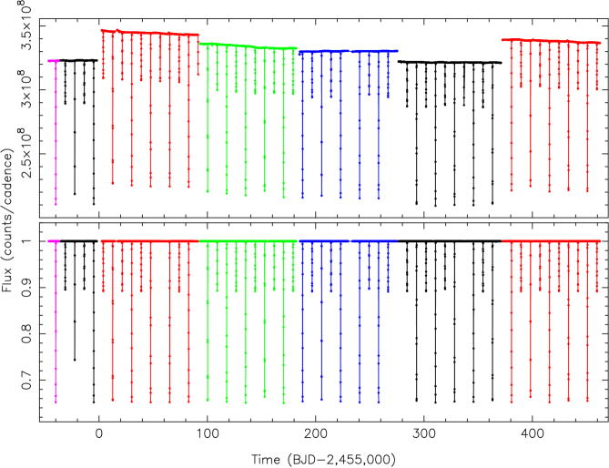
Figure 1: Top: The SAP light curve of KIC 6131659 from Q0 to Q6. Apart from the magenta color for Q0, the colors indicate the season and hence the spacecraft orientation with black for Q1 and Q5, red for Q2 and Q6, green for Q3, and blue for Q4. Bottom: The detrended and normalized light curve. The first primary eclipse in Q1 has an outlier that was given a very low weight. One primary eclipse was missed and a total of six secondary eclipses were only partially covered or missed completely.

The Kepler data processing pipeline (Jenkins et al. 2010a, b) outputs two types of light curves, simple aperture photometry (SAP) light curves and “pre-search data conditioned” (PDC) light curves, which have some of the instrumental trends removed (Smith et al. 2012; Stumpe et al. 2012). While recent versions of the PDC light curves have better detrending, they still have problems removing sudden jumps in the light curves (usually due to cosmic rays). We have also found that the PDC process tends to overcorrect when removing light from contaminating sources. We therefore used the SAP data in this study, and implemented our own detrending algorithm. Each quarter of data is detrended separately. Discontinuities due to cosmic ray hits and gaps in the light curves (usually caused by either monthly data downloads and quarterly rolls) were identified by a visual inspection. The light curves were then divided up into pieces using the discontinuities and gaps as end points. Each piece of the light curve was normalized in a way similar to the way an optical spectrum is normalized to its local continuum. The relatively flat out-of eclipse areas of the light are treated as the “continuum”, and the eclipses are treated as “absorption lines”. Using the fitting tools in the IRAF task ’splot’, an $n$-piece cubic spline interpolating function (where $n$ was typically between 10 and 30) was fit to each piece after the eclipses were masked out using an iterative sigma-clipper. Each light curve piece was divided by the interpolating function, and the normalized pieces were reassembled to make the complete and normalized light curve. The SAP and detrended light curves are shown in Figure 1.

There is a single point in the middle of the first primary eclipse seen in Q1 that is much brighter than it should be, based on the other primary eclipses seen. This outlier is believed to be a result of an error in the cosmic ray rejection routine (J. Jenkins 2011, private communication). A few other similar, but less deviant, outliers were identified in other eclipses. These points were given a very low weight in the analysis described below. Also, although the duty cycle is very high, the light curve is not complete. A secondary eclipse was in progress during a monthly data download in Q2, and one was in progress when the spacecraft performed its quarterly roll at the end of Q2. Likewise in Q5, a secondary eclipse was interrupted by a monthly data download. Since incomplete coverage may introduce errors in the detrending, we excluded all three of these partially covered events entirely. A complete primary eclipse was missed during the spacecraft roll after Q4, and secondary eclipses were missed entirely during the spacecraft rolls following Q2 and Q5.

We have found that the out-of-eclipse variability seen in the Kepler light curves is a good indicator of star-spot activity. As seen in Figure 1, the out-of-eclipse variability in the SAP light curve of KIC 6131659 is at a fairly low level, with a modulation on a several day time scale of $\lesssim 0.2\%$ of the mean flux level. In Figure 2, we compare the SAP light curve of KIC 6131659 to that of the short-period binary KIC 11228612, which is another target in our sample of objects for ground-based follow-up. The period of KIC 1122812 is 2.98046 days, and our spectroscopic results show that the mass of its secondary is about $0.69\,M_{\odot}$, which qualifies it as being “low mass”. Judging from the light curve, it appears that the rotation of the star with the spot is roughly synchronized with the orbit, which is not surprising given the short orbital period. The out-of-eclipse variability in KIC 1122812 is about a factor of 10 larger compared to that seen in KIC 6131659. For comparison, Basri et al. (2011) presented a variability study of a large sample of G and M dwarfs with Kepler data. For stars with roughly periodic variability, the typical amplitude of variability seen in the light curves is $\approx 2$ mmag, which is similar to the level of of variability seen in KIC 6131659.

2.2 Ground-based Photometry

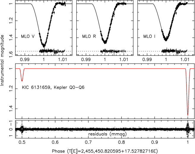
Figure 3: Top: the phased Mount Laguna Observatory $V$-, $R$-, and $I$-band light curves (taken during primary eclipse) and the best-fitting models. The residuals of the fits are shown along the dashed lines. Middle: The phased, detrended, and normalized Kepler light curve (red) and best-fitting model (black). Bottom: The residuals of the model fit to the Kepler data.

KIC 6131659 was observed on 2010 August 7 and 2011 July 6 (UT) using the 0.6m telescope at the Mount Laguna Observatory (near San Diego, California) and a SBIG STL-1001 E CCD camera. Johnson $R$ and Kron $I$ filters were used for the 2010 observations, and Johnson $V$, $R$, and Kron $I$ filters were used for the 2011 observations. The exposure times were 60 seconds for $V$, and 30 to 120 seconds for $R$ and $I$. A total of 109 useful images in $V$, 164 images in $R$, and 195 images in $I$ were obtained. Twilight flats were taken, and dark exposures to match the exposure times of the target images were obtained throughout the night. IRAF was used to make the standard corrections and calibrations for the electronic bias, dark current, and flat-field. The programs DAOPHOT IIe, ALLSTAR, and DAOMASTER (Stetson 1987, 1992a, 1992b; Stetson, Davis, & Crabtree 1991) were used to obtain the differential light curves, which are shown at the top of Figure 3, and presented in Tables 1, 2 and 3.

2.3 Radial and Rotational Velocities

We obtained 13 echelle spectra using the High Resolution Spectrograph (HRS; Tull 1998) and the Hobby-Eberly Telescope (HET; Ramsey et al. 1998) between 2010 August 18 and 2011 July 10 (UT). The instrumental configuration consisted of a resolving power of 30,000, the central echelle rotation angle, the 316 groove mm^-1 cross disperser set to give a central wavelength of 6948 Å, the $2^{\prime\prime}$ science fiber, and two sky fibers. The exposure times were 600 seconds, split into two parts of 300 seconds each to facilitate the removal of cosmic rays. After the electronic bias was removed from each image, pairs of images were combined using the “crreject” option for cosmic ray removal. Spectra were extracted from the resulting two dimensional images using the “echelle” package in IRAF. In this study we used the spectra from the “blue” CCD, which provides a wavelength coverage between about 5100 and 6900 Å. The data are generally of high quality, with signal-to-noise ratios on the order of 100 per pixel near the peak of the blaze functions.

Each night, one of several stars with precise radial velocities taken from the catalog of Nidever et al. (2002) were observed by the HET staff using the same instrumental configuration used for the KIC 6131659 observations. We have a total of 77 spectra of 40 bright mostly G-type stars from our program (including ones from nights when KIC 6131659 was not observed), and using simple cross correlation near the Mg b features we found that the spectrum of the G5V star HD 135101 provided the best match (Figure 4).

The radial velocities were measured using the “broadening function” technique developed by Rucinski (1992, 2002). The broadening functions (BFs) are rotational broadening kernels, where the centroid of the peak yields the Doppler shift and where the width of the peak is a measure of the rotational broadening. For double-lined spectroscopic binaries the BFs generally provide better radial velocity measurements than cross-correlation measurements made with a single template star, especially in cases where the velocity separation of the two stars is close to the velocity resolution of the spectra. See Bayless & Orosz (2006) for details of this process as applied to similar HET spectra. As a check on the process, we measured the radial velocities of all of our standard star observations using the IRAF task fxcor (a cross-correlation routine with a single template spectrum) and using the BFs, where the spectrum of HD 135101 was used as the template in both cases. A comparison of the BF minus fxcor radial velocities shows a median difference of 0.004 km s^-1 and an rms of 0.061 km s^-1. The rms of the differences is comparable to the typical uncertainties in the radial velocity measurements reported by fxcor.

We derived BFs for all 13 observations of KIC 6131659 using HD 135101 as the template star, whose heliocentric radial velocity was taken to be $-38.921$ km s^-1 (Nidever et al. 2002). We found that the derived radial velocities are very insensitive to the spectral type of the template as similar results were obtained using the other (mainly) G-type radial velocity standard stars and from using a spectrum of 61 Cyg A (spectral type K5V). Figure 5 shows four example BFs. Since care was taken to observe near the quadrature phases, we see well-defined peaks corresponding to the primary and secondary stars. In every case, there is a third peak located between the primary and secondary peaks, which occurs at roughly the same heliocentric velocity. For each observation, we compared the BF derived from the sky-subtracted spectrum to the one derived from a spectrum with no sky subtraction and found little, if any change. Also, the BFs of other targets in our sample observed with the same instrumentation show no third peak. Thus we believe this third peak is real and is due to a faint star.

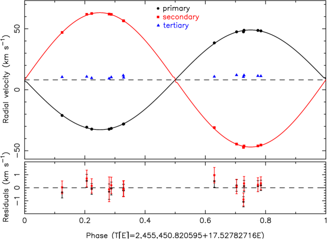
Figure 6: Top: The phased radial velocities of the primary (filled circles), secondary (filled squares), and the third component (filled triangles) and the best-fitting models. The dashed line indicates the systemic velocity of the system. Bottom: The residuals for the fits to the primary and secondary radial velocities.

The BFs were fit to a model consisting of three Gaussian functions to determine the centroids and widths of the peaks. All of the points in each BF were given equal weight, and formal errors on the centroids were found by scaling the uncertainties to give $\chi^{2}_{\nu}=1$. By doing this, the resulting radial velocities derived from the peak centroids (Figure 6) have formal uncertainties of typically 0.05 km s^-1 for the primary and 0.45 km s^-1 for the secondary, respectively. The full width at half maximum (FWHM) of the primary and secondary peaks in the BFs are approximately 10 km s^-1, which is similar to the spectral resolution. Thus the stellar rotational velocities $V_{\rm rot}\sin i$ are not resolved in our observations and are less than about 10 km s^-1.

The BFs of the third star are well separated from the BF peaks of the primary and secondary star. Thus the radial velocities of the primary and secondary should not be biased by the third star. Also, the radial velocities of the third star are roughly constant and there is no indication that the third star interacts with the binary. Thus, it is sufficient to model the radial velocities of the primary and secondary with a standard binary star model. In this case, we modeled the radial velocities for the primary and secondary using a double-sine model where the sines have a common period and systemic velocity and phases 180 degrees apart (the use of a double sine model is justified since we show below that the eccentricity is essentially zero). The uncertainties on the individual measurements were scaled to give $\chi^{2}_{\nu}\approx 1$ for each curve separately. The resulting median uncertainties are 0.45 km s^-1 for the primary and 0.57 km s^-1 for the secondary, respectively. Figure 6 shows the velocities and the best-fitting models. The final adopted radial velocity measurements with the scaled uncertainties are given in Table 4, and the spectroscopic orbital parameters are given in Table 5.

The HET’s HRS used at resolution $R=30,000$ can yield radial velocities with very small errors on sufficiently bright stars, provided that ThAr comparison lamp spectra are obtained in a bracketing fashion, both before and after observations of celestial targets, to detect and correct for “settling” of the cross-disperser grating following configuration changes (S. Mahadevan 2011, private communication). Configuration changes are frequent, since the HET is used in a queue-scheduled mode. In our program, however, ThAr lamp observations were often obtained only before or after observations of a target.

As noted before we have 77 observations of 40 bright stars in our program. We established a grading scale to quantify the stability of the HRS cross-disperser during the observation of the standard stars and their associated ThAr arc exposures, based mainly on the length of time between the configuration change and the actual observations. Nineteen observations were deemed to be trustworthy in the sense that there probably was enough time for the cross disperser to settle before the standard star observation (our best-matched template star HD 135101 is included in that sample). In most of these cases there was an observation of a rapidly rotating B-star or other type of calibration observation just after the configuration change and before the standard star observation. Using HD 135101 as the template, we measured the radial velocity of the other 18 stars in this sample and compared the measured velocities with the velocities from the catalog of Nidever et al. (2002). Although this catalog does not give uncertainties on the individual velocities, the rms scatter of multiple measurements for each star is reported to be less than 100 m s^-1. A histogram showing the distribution of radial velocity differences is shown in Figure 7. The median difference is 0.069 km s^-1 and the rms is 0.157 km s^-1. The distribution can be fit by a Gaussian with a $\sigma$ of 0.130 km s^-1. Based on this analysis we conclude the zero-point of our velocity is consistent with the scale defined by the Nidever et al. (2002) catalog. Furthermore, based on the spread of the radial velocity residual values, the floor on the uncertainties of individual velocity measurements is $\approx 0.16$ km s^-1.

The radial velocities of the third star show no obvious trend. The median heliocentric velocity of the third star is 10.74 km s^-1, and the rms of the 13 measurements is 0.83 km s^-1. This median velocity is close to the systemic velocity of the binary, which is $\gamma=8.142\pm 0.008$ km s^-1, where the uncertainty does not include the error in the velocity zero-point. When one considers the velocity dispersion of stars in the solar neighborhood, which is anywhere between $\approx 20$ and 60 km s^-1, depending on the age (Nordström et al. 2004), the chance that two random stars will have a radial velocity within $\approx 3$ km s^-1 of each other is somewhat small. Also, a wide, hierarchical triple with an outer period of several years could have a velocity difference of a few km s^-1, so it is tempting to conclude the third star is bound to the eclipsing binary. However, the modeling results presented below seem to suggest that the third star is not related to the binary.

2.4 Metallicity and Effective Temperatures

Accurate temperatures and metallicity are essential for the characterization of both stars, but our photometric data does not provide strong constraints on either parameter. The eclipses observed in the light curve yield the ratio $T_{{\rm eff},2}/T_{{\rm eff},1}$, but only weakly constrain the absolute temperatures, and the metallicity cannot be reliably determined photometrically. A spectroscopic analysis can determine the effective temperature, surface gravity, and metallicity, but all three parameters are highly correlated and the results are unreliable in the absence of external constraints. In eclipsing systems the surface gravities can be determined from the light curve, effectively reducing the problem to a more manageable $T_{\rm eff}-{\rm[m/H]}$ degeneracy. Similar to the spectroscopic analysis of Kepler-34 and Kepler-35 (Welsh et al. 2012), we employed the two dimensional cross-correlation routine TODCOR (Zucker & Mazeh 1994) and its extension into three dimensions TRICOR, along with the Harvard-Smithsonian Center for Astrophysics (CfA) library of synthetic spectra to determine the effective temperatures of the binary members and the system metallicity.

The CfA library consists of a grid of Kurucz model atmospheres (Kurucz 2005) calculated by John Laird for a linelist compiled by Jon Morse. The spectra cover a wavelength range of $5050-5360$ Å, and have spacing of $250$ K in $T_{\rm eff}$ and $0.5$ dex in $\log g$ and [m/H]. Initially, TODCOR was used to get the parameters for the primary and secondary. To do this, we cross-correlated the HET/HRS spectra with every pair of templates spanning the range $T_{{\rm eff},1}=[4000,6500]$, $T_{{\rm eff},2}=[3500,6000]$, $\log g_{1,2}=[3.0,5.0]$, ${\rm[m/H]}=[-1.5,+0.5]$, and recorded the mean peak correlation coefficient at each grid point. Next, we interpolated to the peak correlation value in each parameter (but fixed the surface gravities to those found from the photometric analysis) to determine the best-fit parameters for the binary. After the initial TODCOR fits, the third star was accounted for using TRICOR, which yielded improved parameters for the stars in the binary. Given the coarseness of the template grid, we assigned internal errors of $100$ K in $T_{\rm eff}$ and $0.20$ dex in [m/H]. As mentioned above however, the degeneracy between temperature and metallicity could cause correlated errors beyond those quoted here. We explored this by fixing the metallicity to the extremes of the $1$-$\sigma$ errors and assessing the resulting temperature offset. Incorporating these correlated errors, we report the final parameters for KIC 6131659: $T_{{\rm eff},1}=5660\pm 140$ K, $T_{{\rm eff},2}=4780\pm 105$ K, ${\rm[m/H]}=-0.23\pm 0.20$ dex. The calculated light ratio in the wavelength range used in the analysis ($5150-5360$ Å) was $L_{2}/L_{1}=0.105\pm 0.004$. The derived radial velocities were consistent with those derived using the BF analysis, where $K_{1,{\rm TRICOR}}=40.95\pm 0.18$ km s^-1 and $K_{2,{\rm TRICOR}}=54.90\pm 0.22$ km s^-1.

The temperature, gravity, and metallicity of the third star are not well constrained by the TRICOR analysis. The third star contributes relatively little to the fits, and similar correlations were found even when the temperature and gravity of the third star were changed by several grid points. In the end, values of $T_{3}=5000$ K, $\log g_{3}=3.5$, and $[m/H]_{3}=0$ were adopted for the final TRICOR runs.

3 Light Curve Modeling

3.1 Overview

We use the ELC (Eclipsing Light Curve) code (Orosz & Hauschildt 2000) to model the light curves. ELC normally uses the standard Roche geometry to specify the shapes of the stars, and uses specific intensities from model atmospheres. The stellar surfaces are divided up into tiles, and the flux is obtained by numerical integration. When fitting high signal-to-noise light curves such as those provided by Kepler, one obviously needs high precision models, and this is usually done by using more tiles over the stellar surfaces. However, the computational time needed to fully sample parameter space becomes prohibitive, so for well-detached binaries such as KIC 6131659 where the stars are very nearly perfect spheres, another mode of operation was added to ELC where the analytic expressions developed by Kopal (1979), and revisited by Giménez (2006), are used to compute the light curves. Those equations are a function of the fractional radii of the two stars, the inclination, the limb darkening coefficients, and the orbital phase. For each star, the specific intensity at the normal (i.e. at $\mu=1$) is taken from the model atmosphere table for the appropriate temperature and gravity, and intensities for other angles are computed from the limb darkening law, which is either the linear [$I(\mu)=I_{0}(1-x(1-\mu)$] or the “quad” [$I(\mu)=I_{0}(1-x(1-\mu)-y(1-\mu)^{2})$] law. ELC’s “analytic” mode has the advantage in that it is very fast, and large swaths of parameter space can be explored in a relatively short time. The disadvantages are that other effects, such as reflection, ellipsoidal variations, and star spots cannot be easily modeled.

In order to fully match the Kepler long cadence (LC) data, the model light curve is computed at phase intervals that correspond to roughly 1 minute. The model Kepler curve is then binned using simple numerical integration to a bin size of 29.4244 minutes (Gilliland et al. 2010). Such binning is absolutely necessary as the shapes of the model eclipse profiles change noticeably. Since the ground-based light curves are measured using images with much shorter exposure times, no binning is applied for them.

For KIC 6131659, we used a model with 24 free parameters. The inclination $i$, mass ratio $Q=M_{2}/M_{1}$, the $K$-velocity of the primary, and the orbital period $P$ set the scale of the binary (e.g. the semimajor axis $a$ is uniquely determined). The shape and orientation of the orbit is set by the eccentricity $e$, the argument of periastron $\omega$, and a reference epoch, which we take to be the time of the primary superior conjunction $T_{\rm conj}$. The fractional radii $R_{1}/a$ and $R_{2}/a$ set the sizes of the stars. The stellar temperatures are determined by specifying the primary temperature $T_{1}$ and the temperature ratio $T_{2}/T_{1}$. For KIC 6131659, we have two external sources of contaminating light. There is light from the star noticed in the spectroscopy (and possibly physically associated with the binary) which contaminates all of the light curves. This third light is parameterized by the temperature $T_{3}$ and a scaling factor $S$, which is the ratio of the projected area of the third star to the projected area of the primary. There is also contaminating light in the Kepler light curve from stars on the sky whose light leaks into the KIC 6131659 aperture. According to the Kepler Input Catalog, the fraction of light from other sources is a few percent. Since the Kepler pixels are relatively large, the stars that contaminate the Kepler light curve are not a problem for ground-based observations, so a correction is applied only to the model Kepler light curve. The parameter $k$ gives the fractional level of contamination, and the modified flux $f_{\rm new}$ at each phase is given by

$$f_{\rm new}=f+{kf_{\rm med}\over 1+k}$$ (1)

where $f$ is the model flux before correction, and $f_{\rm med}$ is the median flux of the entire model light curve before correction. Finally, we have two limb darkening coefficients for each star for each bandpass. However, since the secondary eclipse is not observed in the $V$, $R$ and $I$ light curves, we don’t fit for those coefficients. This leaves us with a total of 10 coefficients: $x_{1}(K)$ and $y_{1}(K)$ for the primary in the Kepler bandpass, $x_{2}(K)$ and $y_{2}(K)$ for the secondary in the Kepler bandpass, $x_{1}(V)$ and $y_{1}(V)$ for the primary in $V$, $x_{1}(R)$ and $y_{1}(R)$ for the primary in $R$, and $x_{1}(I)$ and $y_{1}(I)$ for the primary in $I$.

3.2 Combined Long Cadence Data Fits

ELC’s genetic algorithm and its Monte Carlo Markov Chain were both used to optimize the model fits to the LC data. Generally speaking, the parameters were allowed to vary over relatively wide ranges. The fits are not sensitive to the adopted value of the primary temperature. Based on the spectral type of around G5V and on the TODCOR analysis, we adopted a range of $5460\leq T_{1}\leq 5860$ K. After some initial runs it was apparent that there was some difficulty with the relative weights between the radial velocity curves and the light curves. Solutions would often converge where the radial velocities were not optimally fit. Some experimentation showed that the optimization worked better when the radial velocity curves were decoupled from the light curves. Thus we fit only the photometric data, using the usual $\chi^{2}$ statistic as the fitness function:

$$\chi^{2}_{\rm photo} = \sum_{i=1}^{23123}{(f(\phi_{i};\vec{a})-f_{\rm obs}(K))^{2}\over\sigma_{i}^{2}}$$ (2)

$$+ \sum_{i=1}^{109}{(f(\phi_{i};\vec{a})-f_{\rm obs}(V))^{2}\over\sigma_{i}^{2}(V)}$$

$$+ \sum_{i=1}^{133}{(f(\phi_{i};\vec{a})-f_{\rm obs}(R))^{2}\over\sigma_{i}^{2}(R)}$$

$$+ \sum_{i=1}^{162}{(f(x_{i};\vec{a})-f_{\rm obs}(I))^{2}\over\sigma_{i}^{2}(I)}$$

where $f(\phi_{i};\vec{a})$ is the model flux at a given phase $\phi_{i}$ for a vector of parameters $\vec{a}$, $f_{\rm obs}$ is the observed value at the same phase, and $\sigma_{i}$ is the uncertainty. The uncertainties on the measurements were scaled to give $\chi^{2}\approx N$ for each data set separately. The resulting median uncertainties are 0.000089 mag, 0.0076 mag, 0.0070 mag, and 0.0090 mag for the Kepler, $V$, $R$, and $I$-band light curves, respectively. The component masses were forced to be consistent with the values found from the separate fits to the radial velocity curves by means of additional $\chi^{2}$ penalties:

$$\chi^{2}_{\rm RV}=(M_{1}-0.922)^{2}/0.007^{2}+(M_{2}-0.685)^{2}/0.005^{2}.$$

The fitness function used for a given model was $\chi^{2}_{\rm tot}=\chi_{\rm photo}^{2}+\chi_{\rm RV}^{2}$. Roughly 2.2 million models were computed from runs of the genetic and Markov chain codes to arrive at the optimal model. The uncertainties on the fitted parameters and derived astrophysical parameters were arrived at by marginalizing the $\chi^{2}$ hypersurfaces over the various parameters of interest. The best-fitting models are shown in Figure 3 and the parameters are summarized in Table 6. The orbital eccentricity is small, but differs from zero. Since the argument of periastron $\omega$ and the eccentricity $e$ are highly correlated, we give the quantity $e\cos\omega$ in Table 6. The contamination in the Kepler light curves due to other light sources leaking into the aperture is found to be zero within the errors.

3.3 Long Cadence Fits to Individual Eclipses

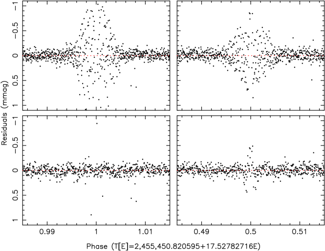
Figure 8: Top: The residuals (in mmag) of the combined fit to the primary eclipse (left) and secondary eclipse (right). The scatter in the out-of-eclipse regions is considerably smaller than it is during eclipse, suggesting systematic issues. Bottom: The residuals (in mmag) obtained after fitting individual pairs of primary and secondary eclipse separately. Here the scatter in the out-of-eclipse phases matches the scatter during eclipse.

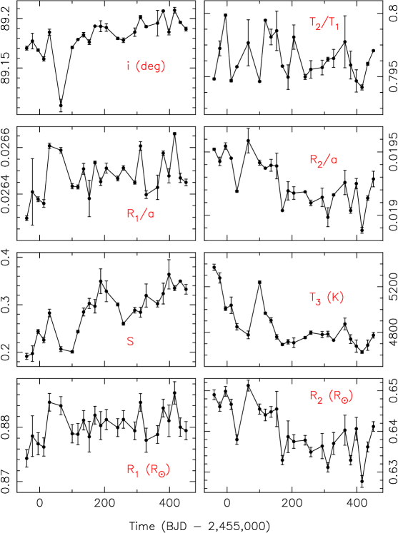
Figure 9: Various fitting and derived parameters derived from the individual light curve segments are shown as a function of the primary eclipse time. From the top, the inclination in degrees, the temperature ratio $T_{2}/T_{1}$, the fractional radii $R_{1}/a$ and $R_{2}/a$, the third light scaling $S$, the third light temperature $T_{3}$ in K, and the primary radius $R_{1}$ in $R_{\odot}$ and the secondary radius $R_{2}$ in $R_{\odot}$ are shown.

Figure 8 (top panels) shows the residuals from the combined Q0-Q6 fit for both the primary eclipse and secondary eclipse. The scatter in the out-of-eclipse regions is somewhat smaller than the scatter in the eclipse phases, which suggests that there may be some small systematic errors. As a check on these systematic issues, we divided the Kepler light curve into 24 segments, each containing a pair of primary and secondary eclipses. Each segment was paired with the ground-based $V$, $R$ and $I$ light curves and modeled separately. Figure 8 (bottom panels) shows the stacked residuals from all 24 fits. In this case the scatter in the in-eclipse and out-of-eclipse phases is similar. Evidently there are small changes from eclipse to eclipse, perhaps caused by small star spots being eclipsed, errors in the light curve normalization, or changes in the contamination level from Quarter-to-Quarter, or all three. The change to each eclipse profile is relatively minor and can be fit for by small changes in the fitting parameters such as the inclination or fractional radii. Table 6 gives the mean, minimum and maximum of each free parameter over the 24 segments, as well as the rms. Figure 9 shows the individual values plotted as a function of time for eight fitted and derived parameters. In most cases, the rms of the individual values from the 24 segments is a bit larger than the formal $1\sigma$ error derived from the combined Kepler light curve, which might be an indication that the formal uncertainties on the values derived from the combined fit are too small. We note that although the fits to each segment are not completely independent owing to the inclusion of the same ground-based data in each one, the spread in the resulting best-fitting parameters that are strongly constrained by the Kepler data, such as the inclination or the fractional radii, should give us some independent measure of the uncertainties. For our final adopted parameters, in most cases we adopt the values found from the median of the 24 individual segment fits, and adopt the rms in those 24 values as conservative $1\sigma$ error. By doing this, for the vast majority of the cases, the difference between the parameter value derived from the combined Q0-Q6 light curve and the median value found from the individual segments is less than $1\sigma$, using the rms as that uncertainty.

3.4 Fits to Short Cadence Data

There is one month of short cadence (SC) data (Gilliland et al. 2010) for KIC 6131659 publically available, namely from the first month of Q5. One primary eclipse and two secondary eclipses are covered. As noted above, the SC data cannot be modeled simultaneously with the LC data owing to the vastly different “exposure times” (i.e. 58.85 seconds vs. 29.4244 minutes). Thus the SC data were treated as one of the individual segments discussed above and modeled with the ground-based light curves. Table 6 gives the parameters. For the most part there is very good agreement between parameters measured from the SC data, the combined LC data, and the individual segments of LC data.

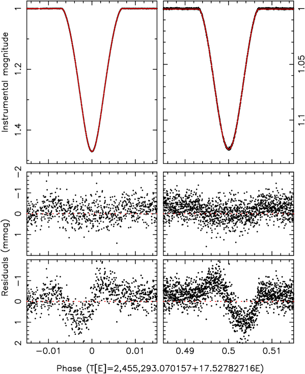
Figure 10: Top: The folded SC data (black) and the best-fitting model (red) of the primary eclipse (left) and secondary eclipse (right). Middle: The residuals (in mmag) of the fit using an eccentric orbit. There are no apparent features near the eclipse phases. Bottom: The residuals (in mmag) obtained after fitting a model with a circular orbit. In this case there are distinctive features at the eclipse phases because the phase difference between the eclipses in the model does not match the phase difference in the observations.

One interesting thing to note about the SC fits is that the eccentricity is small, but is distinctly different from zero: $e\cos\omega=(6.88\pm 0.02)\times 10^{-5}$. Fits with the eccentricity fixed at zero (i.e. circular orbit models) gave significantly worse fits. Figure 10 illustrates the situation. The top panels show the folded SC data and the best-fitting models of both the primary eclipse (left panel) and secondary (right panel). The middle panels show the residuals of the fits for the primary eclipse (left panel) and the secondary eclipse (right panel), and there is a small scatter with an rms on the order of 1 mmag, and no apparent features near the eclipse phases. On the other hand, the residuals from the circular orbit model have distinctive features near the eclipse phases (bottom left for the primary eclipse and bottom right for the secondary eclipse). The phase difference between the primary and secondary eclipse for the eccentric model is 0.500044, or about 67.2 seconds late compared to phase 0.5.

The delay in the secondary eclipse relative to phase 0.5 is due to a combination of light travel time across the orbit and geometry in a slightly eccentric orbit where the true anomaly is not equal to the mean anomaly. The time delay due to light travel time is given by

$$\Delta t_{\rm LT}={PK_{2}\over\pi c}\left(1-{M_{2}\over M_{1}}\right)$$ (3)

where $c$ is the speed of light (Kaplan 2010). Substituting the appropriate numbers from Table 5, we find $\Delta t_{\rm LT}=23.1$ seconds. Thus the delay due to light travel time is roughly one third of the measured delay. The change in the relative timing of primary and secondary eclipse is given by

$$\Delta t_{e}\approx{2Pe\over\pi}\cos\omega$$ (4)

Kaplan (2010), where a factor of two correction has been applied to his Equation (6). Using values in Table 6, the above approximation yields $\Delta t_{e}=66.4$ seconds, which is very close to the value of 67.2 seconds we measured using the short cadence data. Accounting for light travel time, the true delay is $\Delta t_{e,{\rm cor}}=44.1$ seconds. This then gives $e\cos\omega=4.57\times 10^{-5}$. Lucy (2012) recently discussed the process of setting upper limits on the eccentricity where a Bayesian prior on expected tidal evolution of the eccentricity is included. Binaries where $e\ll 1$ but $e\neq 0$ are occasionally expected to occur.

3.5 Discussion of Third Light

We have two distinct parameterizations of third light. The Kepler contamination parameter $k$ accounts for other unrelated stars that are inside the Kepler photometric aperture, but not inside any ground-based apertures. As we discussed earlier, $k$ is very close to zero. The quantities $S$ and $T_{3}$ are used to characterize light from a third star that is present in all of the light curves. There are strong and compelling reasons for including such a star, chief among them the fact that a third star was noticed in the spectra.

Regarding the parameters for that third star noticed in the spectra, the scaling parameter $S$ and the third light temperature $T_{3}$ are somewhat anti-correlated. However, the combined effect of these parameters is such that the amount of light from the third star is roughly equal to the amount of light from the secondary star. This rough equality between the two is consistent with what is seen in the broadening functions (Figure 5). The value of the parameter $S$ indicates the third star’s angular radius is between $\approx 44\%$—$55\%$ the angular radius of the primary. For comparison, the angular (and physical) radius of the secondary is $\approx 72\%$ of the primary’s radius. In addition, the temperature of the third star is somewhat hotter than the secondary (e.g. $T_{3}=4700-5400$ K vs. $T_{2}=4600$ K). If the third star was bound to the eclipsing binary, its physical radius would be only $\approx 50/72=69\%$ the radius of the secondary star. Given that small size, it does not seem likely the third star would be able to produce the same flux as the secondary star if both stars are on the main sequence. On the other hand, if the third star were more distant than the binary, then it could be more luminous than the secondary (as its hotter temperature suggests it should be) but at the same time have roughly the same flux. Thus the fact that the third star has a radial velocity similar to that of the binary may be a coincidence.

Since ELC uses model-atmosphere specific intensities, the overall third light level should be reasonably well constrained given the wide bandpass coverage of the available light curves. Also, wide ranges for the third light parameters were searched, and the solutions converged on a situation where the third light contamination is far from zero. Thus we believe the radii we derive for the primary and secondary should not be biased.

4 Comparison With Model Isochrones and Discussion

Figure 11 shows the positions of the component stars in KIC 6131659 in a mass-radius diagram. The figure also shows three theoretical isochrones from the Dartmouth Stellar Evolution Program (DSEP, Dotter et al. 2008) and the empirical relationship derived by Bayless & Orosz (2006). As noted earlier, most of the low-mass stars with well-measured masses and radii are above the isochrones, meaning the stars are larger than expected, given their masses. In contrast, both stars in KIC 6131659 are on the same isochrone, where the one with an age of 3.5 Gyr, [Fe/H]$=-0.25$, [$\alpha$/Fe]$=0$, and a helium fraction of $Y=0.2537$ formally provides the best fit with $\chi^{2}=0.5287$. The isochrone with an age of 2.5 Gyr, [Fe/H]$=-0.5$, [$\alpha$/Fe]$=0$, and a helium fraction of $Y=0.2537$ has a nearly identical $\chi^{2}$ (0.5397). The metallicities of the best-fitting isochrones match very well the metallicity found from the TODCOR analysis (Table 5). Figure 11 also shows a mass-temperature diagram. Both the primary and secondary are reasonably close to the best-fitting isochrone.

Torres (2007) introduced a parameter $\beta$ which is the correction factor needed to make the model predictions of the radius agree with the measured radius. These are $\beta_{1}=1.001\pm 0.003$ for the primary and $\beta_{2}=0.992\pm 0.009$ for the secondary, respectively. These are consistent with unity, meaning no correction is needed to make the evolutionary models agree with the observations.

Note that the secondary in KIC 6131659 and the primary in Kepler-16 have roughly the same mass as the secondary in RX J0239.1-1028, whereas the radii differ by $\approx 0.1\,R_{\odot}$ (the secondary in RX J2039.1-1028 is the bloated star). At these low masses, neither age differences nor changes in the metallicity will account for the large radius discrepancy. There is therefore at least one other parameter which influences where a star resides in this diagram.

With the recent discoveries of the long-period eclipsing binaries LSPM J1112+7626 (Irwin et al. 2011), Kepler-16 (Doyle et al. 2011), and now KIC 6131659, the observational picture regarding the radii of low-mass stars is becoming more complex. The stars in LSPM J1112+7626 are inflated by about 4%, which indicates that a very long orbital period by itself does not automatically result in agreement with the evolutionary models. Irwin et al. (2011) also showed that LSPM J1112+7626 has a 65 day out-of-eclipse modulation of about 2% which was attributed to star spot activity. As we discussed earlier, KIC 6131659 has an out-of-eclipse modulation of $\lesssim 0.2$%, which presumably translates to a lower level of star spot activity. The primary star in Kepler-16 fits on the model isochrone in the mass-radius diagram, whereas the secondary star does not. There is an $\approx 1\%$ peak-to-peak modulation in the out-of-eclipse light curve of Kepler-16 with periodicity of about 35 days (Winn et al. 2011), where the primary star is presumed to be the source of the modulation. Given these three long-period binaries, one might further speculate that there might be a threshold of stellar activity level past which these stars become inflated.

Feiden, Chaboyer, & Dotter (2011) have recently presented improved evolutionary models which were applied to the three stars in the eclipsing triple system KOI-126 (Carter et al. 2011). A model isochrone with an age of 4.1 Gyr and a metallicity of $[{\rm Fe/H}]=+0.15$ reproduced the observed radii of the stars reasonably well, with formal relative errors between the model predictions and observations of $\leq 0.3\%$. Feiden, Chaboyer, & Dotter (2011) attributed the success of their models to an improved treatment of the equation of state. On the other hand, those same models cannot match the observed radii components of the well-known low-mass binary CM Draconis, even when generous uncertainties in the metallicity are considered. Although the discovery of Kepler-16 was not announced when the paper by Feiden, Chaboyer, & Dotter (2011) was accepted for publication, it can be seen from their Figure 2 that the secondary in Kepler-16 would lie slightly above the model isochrones in the mass-radius diagram. This seems to indicate a real dispersion in the observed mass-radius relation for these fully convective stars.

5 Summary and Thoughts on Future Work

We have analyzed six Quarters of Kepler data along with supporting ground-based photometric and spectroscopic data and obtained precise and accurate values for the masses and radii for both stars in the long-period eclipsing binary KIC 6131659. The component stars in this binary are not bloated, in contrast to nearly all other systems. This suggests that at least one parameter in addition to the mass, age, and metallicity strongly influences the ultimate radius of the star.

More observational work will be needed to better understand the mass-radius relation for low-mass stars. The radii of the components in KIC 6131659 agree with the model predictions for a 3.5 Gyr isochrone. We have shown that the present level of stellar activity in KIC 6131659 is relatively low, which seems to suggest that high levels of spot activity may contribute to the inflated radii found in the short-period low-mass binaries. On the other hand, Kepler-16 has a somewhat higher level of stellar activity, and its primary star also does not appear to be inflated. We speculate that perhaps there is a threshold level of activity past which the stars start to become inflated.

Although the amplitude of any out-of-eclipse modulations may not be a perfect indicator of stellar activity, it is readily observable, especially in Kepler data. Are there binaries with very low levels of out-of-eclipse modulations that nevertheless have stars with inflated radii? Similarly, are there additional binaries like Kepler-16 with spot activity that have at least one star that is not inflated? Ground-based follow-up observations of these binaries, especially the long period systems, can be challenging, however, a sample of a dozen systems could lead to a clearer understanding of the mass-radius relation for low-mass stars.

Table 1: KIC 6131659 $V$-band MLO Photometry

Time	Instrumental $V$	Time	Instrumental $V$	Time	Instrumental $V$
(HJD-2,455,000)	(mag)	(HJD-2,455,000)	(mag)	(HJD-2,455,000)	(mag)
748.75323	$1.3517\pm 0.0076$	748.82965	$1.3727\pm 0.0091$	748.91217	$1.0057\pm 0.0106$
748.75525	$1.3497\pm 0.0076$	748.83167	$1.3517\pm 0.0091$	748.91418	$0.9987\pm 0.0076$
748.75726	$1.3657\pm 0.0076$	748.83368	$1.3477\pm 0.0076$	748.91620	$1.0007\pm 0.0091$
748.75928	$1.3817\pm 0.0076$	748.83771	$1.3077\pm 0.0091$	748.91821	$0.9897\pm 0.0076$
748.76129	$1.3897\pm 0.0076$	748.83972	$1.3057\pm 0.0076$	748.92023	$0.9927\pm 0.0091$
748.76331	$1.3957\pm 0.0091$	748.84174	$1.2937\pm 0.0076$	748.92224	$0.9977\pm 0.0076$
748.76532	$1.4167\pm 0.0091$	748.84375	$1.2837\pm 0.0076$	748.93372	$0.9897\pm 0.0060$
748.76733	$1.4347\pm 0.0091$	748.84576	$1.2677\pm 0.0091$	748.93573	$0.9917\pm 0.0060$
748.76935	$1.4317\pm 0.0091$	748.84778	$1.2567\pm 0.0106$	748.93976	$0.9987\pm 0.0045$
748.77136	$1.4287\pm 0.0106$	748.84979	$1.2467\pm 0.0091$	748.94177	$0.9957\pm 0.0030$
748.77338	$1.4517\pm 0.0076$	748.85181	$1.2287\pm 0.0091$	748.94379	$0.9857\pm 0.0045$
748.77539	$1.4627\pm 0.0091$	748.85382	$1.2217\pm 0.0106$	748.94580	$0.9937\pm 0.0060$
748.77734	$1.4737\pm 0.0106$	748.85583	$1.2067\pm 0.0091$	748.94781	$0.9937\pm 0.0060$
748.77936	$1.4727\pm 0.0106$	748.85986	$1.1927\pm 0.0106$	748.94983	$0.9937\pm 0.0045$
748.78137	$1.4757\pm 0.0091$	748.86188	$1.1737\pm 0.0091$	748.95184	$0.9997\pm 0.0045$
748.78339	$1.4777\pm 0.0121$	748.86389	$1.1597\pm 0.0106$	748.95386	$0.9937\pm 0.0060$
748.78540	$1.4837\pm 0.0106$	748.86591	$1.1507\pm 0.0091$	748.95587	$1.0037\pm 0.0045$
748.78943	$1.4967\pm 0.0136$	748.86792	$1.1377\pm 0.0076$	748.95789	$1.0117\pm 0.0060$
748.79144	$1.5027\pm 0.0091$	748.86993	$1.1417\pm 0.0076$	748.95990	$0.9997\pm 0.0060$
748.79346	$1.4807\pm 0.0166$	748.87195	$1.1137\pm 0.0060$	748.96191	$1.0027\pm 0.0045$
748.79547	$1.5057\pm 0.0151$	748.87396	$1.1037\pm 0.0076$	748.96393	$0.9927\pm 0.0045$
748.79749	$1.4967\pm 0.0151$	748.87598	$1.1007\pm 0.0106$	748.96594	$0.9997\pm 0.0045$
748.79950	$1.4977\pm 0.0151$	748.87799	$1.0987\pm 0.0076$	748.96790	$0.9987\pm 0.0045$
748.80151	$1.4907\pm 0.0121$	748.88202	$1.0757\pm 0.0106$	748.96991	$1.0097\pm 0.0060$
748.80353	$1.4887\pm 0.0136$	748.88403	$1.0577\pm 0.0091$	748.97192	$1.0157\pm 0.0076$
748.80554	$1.4917\pm 0.0091$	748.88605	$1.0627\pm 0.0091$	748.97394	$0.9967\pm 0.0076$
748.80756	$1.4767\pm 0.0106$	748.89008	$1.1037\pm 0.0181$	748.97595	$1.0047\pm 0.0060$
748.80957	$1.4627\pm 0.0076$	748.89203	$1.0417\pm 0.0060$	748.97797	$1.0027\pm 0.0091$
748.81158	$1.4637\pm 0.0060$	748.89404	$1.0347\pm 0.0121$	748.97998	$0.9987\pm 0.0060$
748.81360	$1.4577\pm 0.0091$	748.89606	$1.0387\pm 0.0060$	748.98199	$1.0007\pm 0.0060$
748.81561	$1.4507\pm 0.0091$	748.89807	$1.0297\pm 0.0076$	748.98401	$1.0007\pm 0.0076$
748.81763	$1.4417\pm 0.0076$	748.90009	$1.0437\pm 0.0076$	748.98602	$0.9947\pm 0.0091$
748.81964	$1.4247\pm 0.0091$	748.90210	$1.0187\pm 0.0076$	748.98804	$0.9817\pm 0.0076$
748.82166	$1.4047\pm 0.0076$	748.90411	$1.0017\pm 0.0106$	748.99005	$0.9967\pm 0.0091$
748.82367	$1.4047\pm 0.0091$	748.90613	$1.0007\pm 0.0060$	748.99207	$1.0167\pm 0.0136$
748.82568	$1.4017\pm 0.0091$	748.90814	$1.0037\pm 0.0076$
748.82770	$1.3807\pm 0.0076$	748.91016	$0.9977\pm 0.0091$

Table 2: KIC 6131659 $R$-band MLO Photometry

Time	Instrumental $R$	Time	Instrumental $R$	Time	Instrumental $R$
(HJD-2,455,000)	(mag)	(HJD-2,455,000)	(mag)	(HJD-2,455,000)	(mag)
415.73306	$1.3659\pm 0.0082$	415.92581	$0.9920\pm 0.0093$	748.83038	$1.3366\pm 0.0058$
415.73456	$1.3759\pm 0.0047$	415.92731	$0.9970\pm 0.0082$	748.83240	$1.3286\pm 0.0058$
415.74063	$1.4050\pm 0.0047$	415.93338	$1.0100\pm 0.0070$	748.83441	$1.3136\pm 0.0058$
415.74216	$1.4130\pm 0.0058$	415.93488	$0.9970\pm 0.0058$	748.83643	$1.3046\pm 0.0070$
415.74823	$1.4310\pm 0.0058$	415.94098	$0.9880\pm 0.0082$	748.83844	$1.2846\pm 0.0070$
415.74973	$1.4310\pm 0.0047$	415.94247	$0.9950\pm 0.0082$	748.84039	$1.2836\pm 0.0058$
415.75580	$1.4510\pm 0.0035$	415.94858	$1.0029\pm 0.0070$	748.84241	$1.2746\pm 0.0082$
415.75729	$1.4530\pm 0.0047$	415.95007	$1.0000\pm 0.0058$	748.84442	$1.2526\pm 0.0070$
415.76337	$1.4670\pm 0.0047$	415.95615	$0.9960\pm 0.0058$	748.84644	$1.2396\pm 0.0093$
415.76489	$1.4629\pm 0.0047$	415.95764	$1.0059\pm 0.0047$	748.84845	$1.2436\pm 0.0070$
415.77097	$1.4579\pm 0.0047$	748.75397	$1.3266\pm 0.0058$	748.85046	$1.2296\pm 0.0093$
415.77249	$1.4629\pm 0.0047$	748.75598	$1.3266\pm 0.0070$	748.85248	$1.2146\pm 0.0070$
415.77856	$1.4469\pm 0.0058$	748.75793	$1.3486\pm 0.0070$	748.85449	$1.2056\pm 0.0058$
415.78006	$1.4369\pm 0.0047$	748.75995	$1.3626\pm 0.0070$	748.85651	$1.1926\pm 0.0070$
415.78613	$1.4150\pm 0.0058$	748.76196	$1.3696\pm 0.0070$	748.85852	$1.1786\pm 0.0070$
415.78763	$1.4030\pm 0.0058$	748.76398	$1.3726\pm 0.0047$	748.86053	$1.1776\pm 0.0070$
415.79370	$1.3800\pm 0.0047$	748.76599	$1.3806\pm 0.0070$	748.86255	$1.1566\pm 0.0070$
415.79523	$1.3729\pm 0.0047$	748.76801	$1.4026\pm 0.0070$	748.86456	$1.1486\pm 0.0058$
415.80130	$1.3379\pm 0.0047$	748.77002	$1.4216\pm 0.0105$	748.86658	$1.1326\pm 0.0047$
415.80280	$1.3299\pm 0.0047$	748.77203	$1.4186\pm 0.0082$	748.86859	$1.1416\pm 0.0058$
415.80890	$1.2969\pm 0.0047$	748.77606	$1.4176\pm 0.0070$	748.87061	$1.1116\pm 0.0047$
415.81039	$1.3060\pm 0.0070$	748.77808	$1.4286\pm 0.0070$	748.87262	$1.1116\pm 0.0058$
415.81647	$1.2490\pm 0.0058$	748.78009	$1.4376\pm 0.0093$	748.87463	$1.1116\pm 0.0058$
415.81796	$1.2450\pm 0.0058$	748.78210	$1.4346\pm 0.0093$	748.87665	$1.0956\pm 0.0070$
415.82407	$1.2290\pm 0.0082$	748.78412	$1.4416\pm 0.0128$	748.87866	$1.1236\pm 0.0303$
415.82556	$1.1930\pm 0.0070$	748.78607	$1.4506\pm 0.0082$	748.88269	$1.0736\pm 0.0093$
415.83167	$1.1869\pm 0.0082$	748.78809	$1.4556\pm 0.0082$	748.88470	$1.0566\pm 0.0093$
415.85745	$1.0680\pm 0.0070$	748.79010	$1.4556\pm 0.0093$	748.88672	$1.0596\pm 0.0093$
415.85898	$1.0539\pm 0.0047$	748.79211	$1.4496\pm 0.0128$	748.89075	$1.0496\pm 0.0070$
415.86505	$1.0350\pm 0.0070$	748.79413	$1.4426\pm 0.0105$	748.89478	$1.0316\pm 0.0047$
415.86655	$1.0330\pm 0.0047$	748.79816	$1.4536\pm 0.0105$	748.89679	$1.0416\pm 0.0047$
415.87265	$1.0170\pm 0.0047$	748.80017	$1.4416\pm 0.0128$	748.89880	$1.0276\pm 0.0070$
415.87415	$1.0059\pm 0.0070$	748.80219	$1.4466\pm 0.0093$	748.90082	$1.0336\pm 0.0058$
415.88022	$1.0079\pm 0.0047$	748.80420	$1.4596\pm 0.0082$	748.90283	$1.0146\pm 0.0093$
415.88174	$1.0059\pm 0.0047$	748.80621	$1.4436\pm 0.0058$	748.90485	$1.0206\pm 0.0093$
415.88782	$0.9990\pm 0.0070$	748.80823	$1.4306\pm 0.0058$	748.90686	$1.0196\pm 0.0070$
415.88934	$1.0009\pm 0.0070$	748.81024	$1.4286\pm 0.0082$	748.90881	$1.0136\pm 0.0047$
415.89542	$1.0039\pm 0.0058$	748.81226	$1.4136\pm 0.0047$	748.91083	$1.0066\pm 0.0058$
415.89691	$0.9990\pm 0.0070$	748.81427	$1.4106\pm 0.0082$	748.91284	$1.0006\pm 0.0058$
415.90302	$0.9960\pm 0.0082$	748.81628	$1.4116\pm 0.0058$	748.91486	$0.9906\pm 0.0058$
415.90451	$0.9950\pm 0.0047$	748.81830	$1.4076\pm 0.0070$	748.91888	$1.0036\pm 0.0070$
415.91061	$1.0009\pm 0.0047$	748.82031	$1.3996\pm 0.0070$	748.92090	$0.9956\pm 0.0070$
415.91211	$1.0000\pm 0.0047$	748.82233	$1.3816\pm 0.0070$	748.92291	$1.0106\pm 0.0082$
415.91821	$0.9980\pm 0.0117$	748.82635	$1.3576\pm 0.0082$
415.91971	$1.0020\pm 0.0082$	748.82837	$1.3456\pm 0.0058$

Table 3: KIC 6131659 $I$-band MLO Photometry

Time	Instrumental $I$	Time	Instrumental $I$	Time	Instrumental $I$
(HJD-2,455,000)	(mag)	(HJD-2,455,000)	(mag)	(HJD-2,455,000)	(mag)
415.73608	$1.3535\pm 0.0064$	415.89386	$1.0105\pm 0.0051$	748.81079	$1.4026\pm 0.0116$
415.73758	$1.3505\pm 0.0077$	415.89844	$0.9895\pm 0.0116$	748.81281	$1.3906\pm 0.0103$
415.74365	$1.3975\pm 0.0064$	415.89996	$1.0025\pm 0.0090$	748.81482	$1.3866\pm 0.0103$
415.74515	$1.3875\pm 0.0051$	415.90146	$0.9965\pm 0.0103$	748.81683	$1.3616\pm 0.0103$
415.74664	$1.3935\pm 0.0051$	415.90604	$1.0075\pm 0.0064$	748.81885	$1.3606\pm 0.0090$
415.75125	$1.4185\pm 0.0051$	415.90753	$1.0005\pm 0.0051$	748.82086	$1.3686\pm 0.0103$
415.75424	$1.4145\pm 0.0064$	415.90906	$1.0055\pm 0.0077$	748.82288	$1.3496\pm 0.0103$
415.75882	$1.4285\pm 0.0064$	415.91364	$1.0005\pm 0.0077$	748.82489	$1.3356\pm 0.0090$
415.76031	$1.4305\pm 0.0064$	415.91513	$1.0005\pm 0.0077$	748.82690	$1.3466\pm 0.0116$
415.76181	$1.4305\pm 0.0064$	415.91666	$0.9995\pm 0.0064$	748.82892	$1.3276\pm 0.0064$
415.76639	$1.4225\pm 0.0064$	415.92123	$1.0025\pm 0.0077$	748.83087	$1.3156\pm 0.0077$
415.76791	$1.4325\pm 0.0077$	415.92273	$0.9985\pm 0.0090$	748.83289	$1.2896\pm 0.0090$
415.76941	$1.4275\pm 0.0064$	415.92422	$1.0015\pm 0.0077$	748.83490	$1.2876\pm 0.0090$
415.77399	$1.4165\pm 0.0051$	415.92883	$1.0085\pm 0.0064$	748.83691	$1.2696\pm 0.0129$
415.77548	$1.4125\pm 0.0051$	415.93033	$1.0095\pm 0.0051$	748.83893	$1.2756\pm 0.0090$
415.77698	$1.4065\pm 0.0064$	415.93182	$1.0095\pm 0.0064$	748.84094	$1.2596\pm 0.0090$
415.78159	$1.4005\pm 0.0051$	415.93640	$0.9975\pm 0.0064$	748.84296	$1.2546\pm 0.0077$
415.78308	$1.3835\pm 0.0077$	415.93790	$1.0055\pm 0.0103$	748.84497	$1.2436\pm 0.0090$
415.78458	$1.3905\pm 0.0051$	415.93942	$1.0025\pm 0.0090$	748.84698	$1.2296\pm 0.0090$
415.78915	$1.3785\pm 0.0064$	415.94400	$1.0045\pm 0.0090$	748.84900	$1.2226\pm 0.0090$
415.79065	$1.3625\pm 0.0051$	415.94550	$1.0035\pm 0.0077$	748.85101	$1.2186\pm 0.0090$
415.79214	$1.3745\pm 0.0051$	415.94699	$1.0025\pm 0.0077$	748.85303	$1.1996\pm 0.0090$
415.79672	$1.3415\pm 0.0077$	415.95160	$0.9995\pm 0.0064$	748.85504	$1.1906\pm 0.0116$
415.79825	$1.3435\pm 0.0090$	415.95309	$0.9915\pm 0.0051$	748.85706	$1.1726\pm 0.0116$
415.79974	$1.3265\pm 0.0051$	415.95459	$0.9955\pm 0.0064$	748.85907	$1.1776\pm 0.0103$
415.80432	$1.2965\pm 0.0090$	415.95917	$0.9875\pm 0.0064$	748.86108	$1.1616\pm 0.0103$
415.80582	$1.2995\pm 0.0064$	748.75446	$1.3086\pm 0.0090$	748.86310	$1.1526\pm 0.0116$
415.80731	$1.2875\pm 0.0090$	748.75647	$1.3236\pm 0.0077$	748.86511	$1.1406\pm 0.0090$
415.81192	$1.2685\pm 0.0077$	748.75848	$1.3296\pm 0.0090$	748.86713	$1.1396\pm 0.0077$
415.81342	$1.2525\pm 0.0077$	748.76050	$1.3316\pm 0.0090$	748.86914	$1.1276\pm 0.0064$
415.81491	$1.2475\pm 0.0077$	748.76251	$1.3326\pm 0.0077$	748.87115	$1.1196\pm 0.0103$
415.81949	$1.2245\pm 0.0090$	748.76453	$1.3556\pm 0.0077$	748.87317	$1.1096\pm 0.0090$
415.82098	$1.2155\pm 0.0077$	748.76654	$1.3626\pm 0.0090$	748.87518	$1.1076\pm 0.0090$
415.82248	$1.2035\pm 0.0077$	748.76855	$1.3746\pm 0.0129$	748.87720	$1.0896\pm 0.0090$
415.82709	$1.1985\pm 0.0090$	748.77057	$1.3786\pm 0.0116$	748.88324	$1.0766\pm 0.0103$
415.82858	$1.1735\pm 0.0103$	748.77258	$1.3786\pm 0.0129$	748.88525	$1.0546\pm 0.0103$
415.83008	$1.1815\pm 0.0090$	748.77460	$1.3946\pm 0.0116$	748.88721	$1.1096\pm 0.0180$
415.83466	$1.1455\pm 0.0077$	748.77661	$1.3996\pm 0.0116$	748.88928	$1.0506\pm 0.0244$
415.83618	$1.1505\pm 0.0116$	748.77856	$1.3906\pm 0.0103$	748.89124	$1.0516\pm 0.0090$
415.83768	$1.1315\pm 0.0116$	748.78058	$1.4026\pm 0.0116$	748.89325	$1.0556\pm 0.0167$
415.86047	$1.0575\pm 0.0051$	748.78259	$1.4186\pm 0.0090$	748.89526	$1.0576\pm 0.0077$
415.86200	$1.0465\pm 0.0051$	748.78461	$1.4086\pm 0.0116$	748.89728	$1.0506\pm 0.0077$
415.86349	$1.0445\pm 0.0064$	748.78662	$1.4076\pm 0.0116$	748.89929	$1.0276\pm 0.0090$
415.86807	$1.0275\pm 0.0064$	748.78864	$1.4286\pm 0.0129$	748.90131	$1.0446\pm 0.0103$
415.86957	$1.0245\pm 0.0051$	748.79065	$1.4216\pm 0.0142$	748.90332	$1.0276\pm 0.0090$
415.87109	$1.0215\pm 0.0051$	748.79266	$1.4176\pm 0.0116$	748.90533	$1.0166\pm 0.0103$
415.87567	$1.0205\pm 0.0064$	748.79468	$1.4246\pm 0.0116$	748.90735	$1.0056\pm 0.0116$
415.87717	$1.0105\pm 0.0077$	748.79669	$1.4166\pm 0.0129$	748.90936	$1.0316\pm 0.0090$
415.87866	$1.0105\pm 0.0064$	748.79871	$1.4186\pm 0.0129$	748.91138	$1.0166\pm 0.0090$
415.88327	$1.0035\pm 0.0077$	748.80072	$1.3946\pm 0.0154$	748.91339	$1.0126\pm 0.0116$
415.88477	$1.0105\pm 0.0064$	748.80273	$1.4076\pm 0.0090$	748.91541	$1.0016\pm 0.0129$
415.88626	$1.0095\pm 0.0064$	748.80475	$1.4106\pm 0.0090$	748.91742	$1.0096\pm 0.0090$
415.89087	$1.0035\pm 0.0064$	748.80676	$1.4046\pm 0.0090$	748.91943	$0.9916\pm 0.0103$
415.89236	$1.0125\pm 0.0051$	748.80878	$1.3986\pm 0.0090$	748.92145	$1.0146\pm 0.0090$

Table 4: KIC 6131659 Radial Velocities From BF Analysis

Time	${\rm RV}_{A}$	${\rm RV}_{B}$	${\rm RV}_{C}$
(HJD-2,455,000)	(km s-1)	(km s-1)	(km s-1)
426.81251	$38.44\pm 0.47$	$-31.01\pm 0.60$	$10.77\pm 0.69$
498.61789	$47.52\pm 0.39$	$-47.24\pm 0.50$	$10.55\pm 0.54$
499.63272	$48.27\pm 0.40$	$-45.31\pm 0.50$	$11.19\pm 0.51$
505.59428	$-21.06\pm 0.43$	$47.01\pm 0.50$	$10.46\pm 0.77$
524.55405	$-30.69\pm 0.50$	$61.86\pm 0.64$	$10.74\pm 0.98$
631.02252	$-32.30\pm 0.59$	$62.08\pm 0.95$	$9.22\pm 0.09$
655.96600	$47.50\pm 0.45$	$-44.53\pm 0.56$	$12.04\pm 0.76$
666.90528	$-28.16\pm 0.46$	$56.67\pm 0.61$	$11.72\pm 0.68$
666.92570	$-28.03\pm 0.47$	$56.51\pm 0.61$	$9.99\pm 0.89$
673.92660	$48.79\pm 0.44$	$-46.10\pm 0.54$	$11.87\pm 0.68$
709.78938	$48.68\pm 0.43$	$-46.05\pm 0.54$	$11.36\pm 0.64$
718.78790	$-31.66\pm 0.49$	$61.85\pm 0.63$	$10.29\pm 0.80$
752.70148	$-32.25\pm 0.42$	$62.55\pm 0.55$	$9.63\pm 0.66$

Table 5: KIC 6131659 Spectroscopic Parameters

parameter	value
$P$ (days)	$17.5277\pm 0.0031$
$T_{0}$	$2,455,450.829\pm 0.023$
$e$	0.0 (fixed)
$\omega$ (deg)	$\cdots$
$K_{1}$ (km s-1)	$40.91\pm 0.14$
$K_{2}$ (km s-1)	$55.08\pm 0.18$
$\gamma$ (km s-1)	$8.142\pm 0.008$
$T_{1}$ (K)	$5660\pm 140$
$T_{2}$ (K)	$4780\pm 105$
$[m/H]$ (dex)	$-0.23\pm 0.20$

Table 6: Parameters from Light Curve Fitting

	combined	short	segments
parameter	value	cadence	minimum	maximum	median	rms	adopted
$i$ (deg)	$89.180\pm 0.001$	$89.190\pm 0.003$	89.112	89.208	89.186	0.019	$89.186\pm 0.019$
$Q$	$0.743\pm 0.008$	$0.744\pm 0.007$	0.738	0.746	0.743	0.001	$0.743\pm 0.008$
$K_{1}$ (km s-1)	$40.92\pm 0.25$	$40.95\pm 0.22$	40.77	41.06	40.92	0.05	$40.92\pm 0.25$
$P$ (days)	$17.52782716\pm 0.00000017$	$\cdots$	$\cdots$	$\cdots$	$\cdots$	$\cdots$	$17.52782716(17)$
$T_{\rm conj}$ (HJD 2,455,000+)	$450.820595\pm 0.000002$	$293.070157\pm 0.000008$	$\cdots$	$\cdots$	$\cdots$	$\cdots$	450.820595(2)
$e\cos\omega$ ($\times 10^{-5}$)	$6.94\pm 0.04$	$6.88\pm 0.02$	6.61	7.26	6.98	0.20	$6.88\pm 0.02$
$e\cos\omega$ ($\times 10^{-5}$)	$\cdots$	$\cdots$	$\cdots$	$\cdots$	$\cdots$	$\cdots$	$4.57\pm 0.02$
$R_{1}/a$	$0.026492\pm 0.000009$	$0.026505\pm 0.000023$	0.026296	0.026660	0.026460	0.000086	$0.026460\pm 0.000086$
$R_{2}/a$	$0.019223\pm 0.000009$	$0.019104\pm 0.000032$	0.018880	0.019589	0.019221	0.000182	$0.019221\pm 0.000182$
$T_{1}$ (K)	$5721\pm 5$	$5834\pm 20$	5659	5839	5789	50	$5789\pm 50$
$T_{2}/T_{1}$	$0.79862\pm 0.00099$	$0.79383\pm 0.00072$	0.79415	0.79986	0.79596	0.00158	$0.79596\pm 0.00158$
$T_{2}$ (K)	$4569\pm 18$	$4631\pm 20$	4526	4642	4609	32	$4609\pm 32$
$T_{3}$ (K)	$5258\pm 5$	$4702\pm 60$	4627	5371	4779	195	$4779\pm 195$
$S$	$0.1700\pm 0.0010$	$0.330\pm 0.028$	0.191	0.364	0.293	0.051	$0.293\pm 0.051$
$k$	$\leq 0.001$	$\leq 0.0022$	0.00000	0.00451	0.00070	0.00117	$\leq 0.001$
$x_{1}(K)$	$0.517\pm 0.006$	$0.469\pm 0.020$	0.400	0.685	0.490	0.059	$0.490\pm 0.059$
$y_{1}(K)$	$0.020\pm 0.010$	$0.072\pm 0.036$	$-0.157$	0.269	$0.050$	0.105	$0.050\pm 0.105$
$x_{2}(K)$	$0.703\pm 0.014$	$0.441\pm 0.047$	0.365	0.938	0.623	0.137	$0.623\pm 0.137$
$y_{2}(K)$	$-0.129\pm 0.022$	$0.327\pm 0.080$	$-0.497$	0.344	$0.030$	0.214	$0.030\pm 0.214$
$x_{1}(V)$	$0.630\pm 0.317$	$0.690\pm 0.308$	0.487	0.939	0.787	0.133	$0.630\pm 0.317$
$y_{1}(V)$	$0.190\pm 0.528$	$-0.012\pm 0.467$	$-0.353$	0.290	$-0.099$	0.194	$0.190\pm 0.520$
$x_{1}(R)$	$0.852\pm 0.098$	$0.856\pm 0.112$	0.737	0.944	0.866	0.042	$0.852\pm 0.098$
$y_{1}(R)$	$-0.495\pm 0.290$	$-0.480\pm 0.297$	$-0.500$	$-0.258$	$-0.500$	0.062	$-0.495\pm 0.290$
$x_{1}(I)$	$0.510\pm 0.089$	$0.626\pm 0.124$	0.512	0.678	0.602	0.046	$0.510\pm 0.089$
$y_{1}(I)$	$-0.487\pm 0.215$	$-0.496\pm 0.283$	$-0.500$	$-0.322$	$-0.500$	0.036	$-0.487\pm 0.215$
$M_{1}$ ($M_{\odot}$)	$0.922\pm 0.007$	$0.924\pm 0.007$	0.912	0.927	0.922	0.002	$0.922\pm 0.007$
$M_{2}$ ($M_{\odot}$)	$0.685\pm 0.005$	$0.686\pm 0.004$	0.683	0.687	0.685	0.001	$0.685\pm 0.005$
$R_{1}$ ($R_{\odot}$)	$0.8808\pm 0.0018$	$0.8816\pm 0.0019$	0.8743	0.8863	0.8800	0.0028	$0.8800\pm 0.0028$
$R_{2}$ ($R_{\odot}$)	$0.6391\pm 0.0013$	$0.6355\pm 0.0016$	0.6277	0.6513	0.6395	0.0061	$0.6395\pm 0.0061$
$a$ ($R\,M_{\odot}$)	$33.247\pm 0.065$	$33.264\pm 0.047$	33.246	33.292	33.247	0.012	$33.247\pm 0.065$

Figure 2: Top: A portion of the scaled SAP light curve of KIC 6131659 from Q3. The dip near day 104.5 is a single point, and is likely an instrumental artifact. In addition to long-term decrease that is probably instrumental, there is a modulation in the out-of-eclipse flux at the level of 0.1 to 0.2%. Bottom: A portion of the scaled SAP light curve of KIC 11228612 from the same time period. Note that the $y$-axis scale is ten times larger compared to the top panel. Here we see variability in the out-of-eclipse regions of about 2%.

Figure 4: The normalized spectra of the G5V star HD 135101 (top, shifted upward) and KIC 6131659 (bottom) in the region near the Mg b lines. This particular observation of KIC 6131659 has been Doppler-shifted to match the velocity of HD 135101.

Figure 5: The “broadening functions” (BFs) from four observations, with the UT dates indicated. The lags have been corrected to the heliocentric frame. The peaks due to the primary (P), secondary (S) and the third component (T) are indicated in the upper left panel.

Figure 7: The distribution of the differences between the measured radial velocity and the catalog velocity (Nidever et al. 2002) for the 18 template star observations. The median value is 0.069 km s^-1 and the rms is 0.157 km s^-1. The smooth curve is a Gaussian with a $\sigma$ of 0.130 km s^-1.

Figure 11: Top: A mass-radius diagram for well-characterized low-mass stars in eclipsing binaries (measurements from Torres, Andersen, & Giménez (2010) and cited references, Carter et al. (2011), and Irwin et al. (2011)). The evolutionary models are from Dotter et al. (2008). Also shown is the empirical relation derived by Bayless & Orosz (2006). The location of the components in KIC 6131659 are shown in red with the primary denoted by an ’A’ and the secondary denoted by a ’B’. Note that the symbol for KIC 6131659 B nearly covers up the symbol for the primary in Kepler-16. The mass-radius relationship from other studies are included on the figure for comparsion. Only well-studied figures with low error bars are included. Some recent work has identified more potential low mass binaries for study (see e.g. Bhatti et al. 2010; Becker et al. 2011), but have not yet produced well constrained values for the masses for these targets, and are thus not included. Bottom: A mass-temperature diagram showing the positions of KIC 6161659 against the same three isochrones that are displayed in the top panel, where the effective temperatures were derived from the TODCOR analysis.

References

- Basri et al. (2011) Basri, G., Walkowicz, L. M., Batalha, N., Gilliland, R., L., et al. 2011, ApJS, 141, 20
- Batalha et al. (2010) Batalha, N. M., Borucki, W. J., Koch, D. G., Bryson, S. T., Haas, M. R., et al. 2010, ApJ, 713, L109
- Bayless & Orosz (2006) Bayless, A. J. & Orosz, J. A. 2006, ApJ, 651, 1155
- Becker et al. (2011) Becker, A. C., Bochanski, J. J., Hawley, S. L., Ivezić, Ž., Kowalski, A. F., Sesar, B., & West, A. A. 2001, ApJ, 731, 17
- Bhatti et al. (2010) Bhatti, W., Richmond, M. W., Ford, H. C., & Petro, L. D. 2010, ApJS, 186, 233
- Bopp (1974) Bopp, B. W. 1974, ApJ, 193, 389
- Borucki et al. (2010) Borucki, W. J., Koch, D., Basri, G., Batalha, N., Brown, T., et al. 2010, Science, 327, 977
- Çakirli, İbanoǧlu, & Dervişoǧlu (2011) Çakirli, Ö., İbanoǧlu, C., & Dervişoǧlu, A. 2011, Rev. Mexicana Astron. Astrofis., 46, 363
- Caldwell et al. (2010) Caldwell, D. A., Kolodziejczak, J. J., Van Cleve, J. E., Jenkins, J. M., Gazis, et al. 2010, ApJ, 713, L92
- Carter et al. (2011) Carter, J. A., Fabrycky, D. C., Ragozzine, D., Holman, M. J., Quinn, S. N., et al. 2011, Science, 331, 562
- Coughlin et al. (2011) Coughlin, J. L., López-Morales, M., Harrison, T. E., Ule, N., & Hoffman, D. I. 2011, AJ, 141, 78
- Devor et al. (2008) Devor, J., Charbonneau, D., Torres, G., Blake, C. H., et al. 2008, ApJ, 687, 1253
- Dotter et al. (2008) Dotter, A., Chaboyer, B., Jevremović, D., Kostov, V., Baron, E., Ferguson, J. W. 2008, ApJS, 178, 89
- Doyle et al. (2011) Doyle, L. R., Carter J. A., Fabrycky, D. C., Slawson, R. W., et al. 2011, Science, 333, 1602